Quantum Gravity Corrections to the Mean Field Theory of Nucleons

At present there are various different approaches to quantum gravity. It is important to know the universal features of all these different approaches to quantum gravity. It is expected from almost all of these approaches that the geometric of space-time has an intrinsic minimal length associated with it [7]. Any quantum theory of gravity, should be consistent with black hole physics. Now it is known that we need higher energies to probe smaller length scales. The energy to probe Planckian region of space is equal to the energy needed to form a black hole in that region of space. Thus, if we try to make Planckian measurements, we will form mini black holes, which will prevent us from making such measurements [1, 2]. So, it is not possible to probe space-time below Planck scale, and Planck length acts as an intrinsic minimal length in space-time. Such a minimal length exists even in asymptotically safe gravity [20] and conformally quantized quantum gravity [21]. Such a minimal length in the background geometry of space-time also exists in loop quantum gravity [16, 17, 18, 19] because of polymer quantization, as the polymer length acts as a minimal length in loop quantum gravity.

It can be argued that there exists a minimal length of the order of Planck length in the background geometry of space-time [7]. However, it is possible for this minimal length to be of several order of magnitude larger than the Planck length. This is because in string theory it is possible to relate this minimal length to the string length [3, 4]. In fact, it can be demonstrated that this minimal measurable length $l_{min}$ can be directly related to string length $l_{s}=\alpha^{\prime}$ as $l_{min}=g_{s}^{1/4}l_{s}$, with $g_{s}$ as the string coupling constant [5, 6]. Even though it is possible to obtain point like $D0$-branes due to non-perturbative effects, it has been demonstrated that there is a minimal length even with such non-perturbative point like objects. The minimal length in string theory, with such non-perturbative objects is related to the string length as $l_{min}=l_{s}g_{s}^{1/3}$ [7, 8]. So, by adjusting the string coupling constant, the string length can be several orders larger than the Planck length.

Another reason is that string theory is invariant under T-duality. So, for a string compactified on a circle with radius $R$, the mass states do not change under the transformation $R\to l_{s}^{2}/R$, and $n\to w$, where $n$ are the Kaluza-Klein modes and $w$ are the winding modes. Thus, it is not possible to obtain new information by going below a zero point length in string theory compactified on a compact geometry [7]. It is also possible to construct an effective path integral for the center of mass of the strings compactified on a circle, by neglecting all the string oscillation modes. This effective path integral can be used to obtain suitable propagators in such a theory, and it can be explicitly demonstrated that such propagators are invariant under T-duality [9, 10]. Thus, there is an intrinsic zero point length, (larger than the Planck length) associated with such propagators, even if the string oscillation modes are neglected. It may be noted as the double field theory is constructed using the T-duality [11, 12], it is expected that a such zero point length can also occur in the double field theory. It has been demonstrated that such a zero point length in double field theory can have important consequences for the generalized geometries used in string theory [13]. It may be noted that such a minimal length larger than the Planck length can make it possible for the mini black holes to form in particle physics colliders (due to the lowering of Planck scale) [14, 15]. Thus, the existence of such a minimal length, larger than the Planck length, can have interesting physical consequences.

It is possible for such a minimal length to deform the low energy quantum mechanical systems [22, 23]. This deformation of such low energy quantum mechanical systems can detected by ultra precise measurements of Landau levels and Lamb shift in atomic systems [24]. It has also been proposed that such a deformation of low energy quantum mechanics can be detected using an opto-mechanical setup [25]. It is possible to use a gravitational spectrometer to measure the interaction between neutrons and a gravitational field [26, 27]. As this system will also be deformed by the deformation of quantum mechanics from a minimal length, it is possible to use a gravitational spectrometer to measure the effects of minimal length on such a system [28]. Thus, the deformation of the Heisenberg algebra from minimal measurable length can have interesting low energy consequences.

It may be noted that it is possible to study several different forms of deformation of quantum mechanics [29, 30, 31, 32, 33]. We will use a specific form of deformation [38, 39, 41, 42, 43, 44, 45, 46, 47, 40, 48], which is consistent with the effects produced from various different theories, such as non-locality [49], doubly special relativity [50], deformed dispersion relations in the bosonic string theory [51], Horava-Lifshitz gravity [52, 53], discrete space-time [54], models based on string field theory [55], space-time foam [56], spin-network [57], and noncommutative geometry [58]. We will study the effects of such a deformation in the mean field theory potential for a system of nucleons. Such a mean field theory potential for a system of nucleons can be described by a Woods-Saxon potential [59, 60, 61, 62, 63]. It may be noted that the correction to the Woods-Saxon potential from the simplest deformation of the Heisenberg algebra has been studied [68, 69, 70, 71, 72]. However, here we will deform the Schrödinger’s equation with this potential using the deformation of the Heisenberg algebra, with linear terms [38, 39, 41, 42, 43, 44, 45, 46, 47, 40, 48]. It may be noted that the deformation of the angular momentum algebra consistent with this algebra has been studied [73, 74], and we will use this deformation of the angular momentum algebra to analyze the deformed Woods-Saxon potential.

In this section, we will analyze the corrections to the mean field theory potential for a system of nucleons from a deformation of the Heisenberg algebra. As the mean field theory potential for a system nucleons is represented by the Woods-Saxon potential [59, 60, 61, 62, 63], we will analyze such corrections to the Woods-Saxon potential. Even though there are various different models of nuclear potential, the advantage of using Woods-Saxon potential is that it explain a larger set of magic numbers [59, 60, 61, 62, 63]. Furthermore, this potential has been used to explain a large number of nuclear systems. The Wood-Saxon nuclear potential can explain the effect of the chiral magnetic field in relativistic heavy-ion collisions [64]. The prolate-shape predominance of the nuclear ground-state deformation for two thousand nuclei has been obtained using this potential [65]. This potential has been used to investigate the toroidal and superdeformed configurations in light atomic nuclei [66]. It has also been used to explain the hyperfine structure of heavy ions [67]. As the Wood-Saxon nuclear potential has been used to investigate a large number of nuclear systems, it is possible to test its deformation using such nuclear systems. So, we will analyze its corrections from the deformation of the Heisenberg algebra. The Woods-Saxon potential can be expressed as [59, 60, 61, 62, 63]

$$V_{WS}(r)=-\frac{V_{0}}{1+exp(\frac{r-a_{0}}{a})},~a<<a_{0}$$

(1)

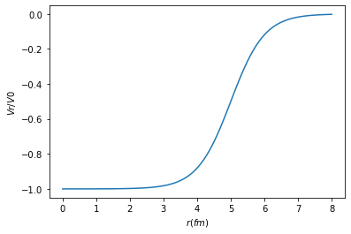
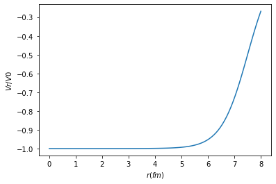
Here $a_{0}$ denotes radius of nucleus, which in turn is connected to the mass number by $a_{0}=cA^{1/3}$ with $c=1.25fm$. The parameter $a$ characterize the thickness of superficial layer. Furthermore, $V_{0}$ represents the depth of the potential well. We have plotted the form of this potential in Fig. 1. We plotted the potential for two different radius, corresponding to two different mass numbers. The potential is similar to infinite potential well, except that the walls are smooth. The plot on the left is drawn for a nucleus with mass number $A=125$ and the plot on the right has been drawn for $A=216$. It may be observed that with increasing mass number, the potential resembles that of a potential of a potential well.

Now we will analyze the correction to this Woods-Saxon potential from a deformation of the Heisenberg algebra with a linear term [38, 39, 41, 42, 43, 44, 45, 46, 47, 40, 48]. It may be noted that this deformation is consistent with various different theories, such as non-locality [49], doubly special relativity [50], deformed dispersion relations in the bosonic string theory [51], Horava-Lifshitz gravity [52, 53], discrete space-time [54], models based on string field theory [55], space-time foam [56], spin-network [57], and noncommutative geometry [58]. This deformation can be explicitly written as [38, 39, 41, 42, 43, 44, 45, 46, 47, 40, 48]

$$[x_{i},p_{j}]=i\hbar\left[\delta_{ij}-\alpha\left(p\delta_{ij}+\frac{p_{i}p_{j}}{p}\right)+\beta^{2}\left(p^{2}\delta_{ij}+3p_{i}p_{j}\right)\right]$$

(2)

Now this deformation of the Heisenberg algebra will produce a deformation in the coordinate representation of the momentum operator from $p$ to $p\left(1-\langle\mathcal{C}\rangle\right)$, where

$$\langle\mathcal{C}\rangle=\alpha\langle p\rangle-\beta^{2}\langle p\rangle^{2}$$

(3)

It is important to define a coefficient $\lambda$ as

$$\lambda=\left(1-\langle\mathcal{C}\rangle\right)$$

(4)

It may be noted here that for $\alpha\langle p\rangle>\beta^{2}\langle p\rangle^{2}$, $\langle\mathcal{C}\rangle>0$, and $\lambda<1$. However, for $\alpha\langle p\rangle<\beta^{2}\langle p\rangle^{2}$, $\langle\mathcal{C}\rangle<0$, and $\lambda>1$. So, when $\lambda<1$, the linear term dominates and when $\lambda>1$, the quadratic term dominates. The corrections vanish at $\lambda=1$, which corresponds to $\langle\mathcal{C}\rangle=0$. It may be noted that the corrections to the Woods-Saxon potential from such a quadratic term have already been analyzed [68, 69, 70, 71, 72]. However, here we will analyze it for both linear and quadratic terms. The deformation of the momentum operator by $\langle\mathcal{C}\rangle$ in turn deforms the angular momentum algebra for this system as [73, 74]

	$\displaystyle L^{2}|plm\rangle=\hbar^{2}l(l+1)\left(1-\langle\mathcal{C}\rangle\right)^{2}|plm\rangle~$		(5)
	$\displaystyle L_{z}|plm\rangle=\hbar m\left(1-\langle\mathcal{C}\rangle\right)|plm\rangle~$		(6)

We will use these modified angular momentum operators to explicitly analyze the corrections to the Woods-Saxon potential. It may be noted that the original radial Schrödinger’s equation with Woods-Saxon potential is given by [59, 60, 61, 62, 63],

$$\frac{d^{2}\mathcal{R}}{dr^{2}}+\frac{2}{r}\frac{d\mathcal{R}}{dr}+\frac{2m}{\hbar^{2}}\left[E-V_{WS}-\frac{\hbar^{2}l(l+1)}{2mr^{2}}\right]\mathcal{R}=0$$

(7)

Now we can write the deformation of this Schrödinger’s equation from a deformation of the Heisenberg algebra as [73, 74]

$$\left(1-\langle\mathcal{C}\rangle\right)^{2}\left[\frac{d^{2}\mathcal{R}}{dr^{2}}+\frac{2}{r}\frac{d\mathcal{R}}{dr}\right]+\frac{2m}{\hbar^{2}}\left[E-V_{WS}-\frac{\hbar^{2}l(l+1)}{2mr^{2}}\left(1-\langle\mathcal{C}\rangle\right)^{2}\right]\mathcal{R}=0$$

(8)

We will use Nikiforov-Uvarov method [75, 76] to solve the deformed Schrödinger’s equation for the Woods-Saxon (see Appendix A). We start with $R={U(r)}/{r}$, we can write the deformed Schrödinger’s equation with Woods-Saxon potential as

$$\frac{d^{2}U}{dr^{2}}+\frac{2m}{\hbar^{2}\lambda^{2}}\left[E-V_{WS}(r)-V_{l}(r)\right]U=0$$

(9)

Here we have expressed the total effective potential as a sum of the original Woods-Saxon potential $V_{WS}(r)$ and the deformation of the potential $V_{l}(r)$ as

	$\displaystyle V_{eff}=V_{l}(r)+V_{WS},$		$\displaystyle V_{l}(r)=\frac{\hbar^{2}l(l+1)}{2mr^{2}}\lambda^{2}$
	$\displaystyle V_{WS}=\frac{V_{0}}{1+exp(\frac{r-a_{0}}{a})}.$				(10)

Now with the two new variables $x=(r-a_{0})/a_{0},$ and $~\alpha={a_{0}}/{a}$, and we can simplify the effective potential using Pekeris approximation (see Appendix B). The deformed Schrödinger’s equation, can be written as a ordinary Schrödinger’s equation, where the Woods-Saxon potential has been replaced by this effective potential

$$\frac{d^{2}U}{dr^{2}}+\frac{2m}{\lambda^{2}\hbar^{2}}\left[E-\Delta_{\lambda}A_{0}+\frac{V_{0}-\Delta_{\lambda}A_{1}}{1+exp(\frac{r-a_{0}}{a})}-\frac{\Delta_{\lambda}A_{2}}{[1+exp(\frac{r-a_{0}}{a})]^{2}}\right]$$

(11)

We can solve the deformed Schrödinger’s equation by Nikiforov-Uvarov method [75, 76] by introducing the dimensionless quantities

	$\displaystyle\epsilon^{2}(\lambda)=-\frac{2ma^{2}(E-\Delta_{\lambda}A_{0})}{\lambda^{2}\hbar^{2}},$		$\displaystyle\beta^{2}(\lambda)=\frac{2ma^{2}(V_{0}-\Delta_{\lambda}A_{1})}{\lambda^{2}\hbar^{2}},$
	$\displaystyle\qquad\gamma^{2}=\frac{2ma^{2}(\Delta_{\lambda}A_{2})}{\lambda^{2}\hbar^{2}}.$				(12)

The term $\Delta_{\lambda}$ scales as $\lambda^{2}$, making $\gamma$ which scales as $\Delta_{\lambda}/\lambda^{2}$ independent of $\lambda$. So, using a new variable $z=[1+\exp(({r-a_{0}}){a}^{-1})]^{-1}$, we can write the deformed Schrödinger’s equation as

$$\frac{d^{2}U(z)}{dz^{2}}+\frac{1-2z}{z(1-z)}\frac{dU(z)}{dz}+\frac{-\epsilon^{2}(\lambda)+\beta^{2}(\lambda)z-\gamma^{2}z^{2}}{[z(1-z)]^{2}}U(z)=0$$

(13)

We can explicitly obtain the solution to this deformed Schrödinger’s equation (see Appendix C). We can also obtain condition for the bound states to exist in this deformed Woods-Saxon potential as $-n^{{}^{\prime}2}<[\beta^{2}(\lambda)-\gamma^{2}]<n^{{}^{\prime}2},$ with $n^{{}^{\prime}}=-n+{({1+4\gamma^{2}})^{1/2}-1}/{2}$. The bound states only exist for $n^{{}^{\prime}}>0$. Using the value of $\gamma$, we can write this bound as $0\leq 2n\leq(1+{192a^{4}l(l+1)}{a_{0}^{-4}})^{1/2}-1$. Thus, we obtain finite values of $n$ for bound states. Now using $\beta(\lambda),\gamma,A_{0},A_{1},A_{2}$, we can obtain the upper and lower bounds of the potential $V_{0}$.

$$\frac{8\Delta_{\lambda}}{\alpha}-\frac{\hbar^{2}}{2ma^{2}}n^{{}^{\prime}2}<V_{0}<\frac{8\Delta_{\lambda}}{\alpha}+\frac{\hbar^{2}}{2ma^{2}}n^{{}^{\prime}2}$$

(14)

Using this bound it is possible to explicitly obtain the corrected energy of the system as (Appendix C)

$\displaystyle E_{nl}(\lambda)$

$\displaystyle=$

$\displaystyle\frac{\hbar^{2}l(l+1)\lambda^{2}}{2ma_{0}^{2}}\xi_{0}-\frac{\hbar^{2}}{2ma^{2}}\left[\frac{\xi_{1}}{16}+\frac{\xi_{2}}{\xi_{1}}+\frac{mV_{0}a^{2}}{\hbar^{2}}\right],$

(15)

where $\xi_{0}=1+12a^{2}a_{0}^{-2}$, $\xi_{1}=[(1+192l(l+1)a^{4}a_{0}^{-4})^{1/2}-2n-1]^{2}$ and $\xi_{2}=4[ma^{2}V_{0}\hbar^{-2}-4l(l+1)\lambda^{2}a^{3}a_{0}^{-3}]^{2}$.

Now we can write the wave functions for the deformed Woods-Saxon potential. The general wave function can be expressed as

$$\psi(z)=\Phi(z)y(z)$$

(16)

where $\Phi(z)=z^{\epsilon(\lambda)}(1-z)^{\zeta}$ with $\zeta=\sqrt{\epsilon^{2}(\lambda)-\beta^{2}(\lambda)+\gamma^{2}}$. This wave function can be simplified by using the Rodrigues relation and Jacobi polynomials (Appendix D). So, using $\alpha=2\epsilon$ and $\beta=2\sqrt{\epsilon^{2}(\lambda)\beta^{2}(\lambda)+\gamma^{2}}$, we can write the radial wave function as

$\displaystyle\mathcal{R}_{nl}(z)=K_{nl}z^{\epsilon(\lambda)}(1-2z)(1-z)^{\sqrt{\epsilon^{2}(\lambda)-\beta^{2}(\lambda)+\gamma^{2}}}P_{n}^{(2\epsilon(\lambda),2\sqrt{\epsilon^{2}(\lambda)-\beta^{2}(\lambda)+\gamma^{2}}}$

(17)

where $K_{nl}$ is the normalizing constant. It may be noted that the value $\lambda=1$, corresponds to $\mathcal{\langle C\rangle}=0$, which produces the wave functions for original Schrödinger’s equation with Woods-Saxon potential. Thus, $\lambda$ measures the corrections to this equation from the deformation of the Heisenberg algebra. We have presented the wave functions for the deformed Schrödinger’s equation for the iron nucleus $(^{56}Fe)$ in Fig. 2. The parameters for this system are $a_{0}=1.285fm$, $a=0.65fm$, $V_{0}=(40.5+0.13A)MeV=47.78MeV,R=R_{0}A^{\frac{1}{3}}=4.9162fm,m_{core}=56u,m_{n}=1.00866u$. We plot the wave functions for $l=0$ and $n=0,1,2$ with $\lambda=1$ (original Schrödinger’s equation), and for $\lambda>1$ and $\lambda<1$. It may be noted that as we are using a general deformation of the Heisenberg algebra [38, 39, 41, 42, 43, 44, 45, 46, 47, 40, 48], it is possible to take both these values. They correspond to the modification terms in the deformed Heisenberg algebra.

In this paper, we have analyzed the correction to the mean field theory potential for a system of nucleons from a deformed Heisenberg algebra representing quantum gravitational effects. As the mean field potential for the nucleons can be described by the Woods-Saxon potential, we analyzed such a deformation of the Schrödinger’s equation for the Woods-Saxon potential. We used a Nikiforov-Uvarov method to solve such a deformed Schrödinger’s equation. These solutions were numerically analyzed. It was demonstrated that the deformed Schrödinger’s equation could be analyzed as an ordinary deformed Schrödinger’s equation with an effective potential. This effective potential was expressed as a sum of the deformed and the original Woods-Saxon potentials. We explicitly obtained the corrections to the energy eigenstates of this system. The corrections to the wave function of this system were also obtained. It would be interesting to use these results explicitly to analyze various different nuclear systems. Thus, we can use the data from different nuclear processes to analyze such corrections. It could be possible to use such precise nuclear data to constrain quantum gravity theories. Now such a modification of the wave function will modify the dynamics in most physical models described by Woods-Saxon potential. We can use this wave function to calculate the dwell time in tunneling, which can then be related to the half life of the nucleus [34, 35, 36, 37]. This dwell time is the average time spend by a particle in a given region. Now for a nuclear system, with incident flux $j$, this dwell time between $z_{1}$ and $z_{2}$ is given by [34, 35]

$$\tau_{D}=\frac{1}{j}\int_{z_{1}}^{z_{2}}dz|\psi(z)|^{2},$$

(18)

where $\psi(z)$ is the wave functions for the Woods-Saxon potential. Now as this deformation of the Woods-Saxon potential has modified this wave function, it would modify the dwell time, and this in turn would modify the half life of the nucleus [34, 35, 36, 37]. This modification can be explicitly obtained by using the corrected wave function given by Eq. (16). Such modification could be experimentally detected in future experiments. It would be interesting to investigate the effect of such deformation on various nuclear systems, and use the experimental data to constraint the minimal length used to deform such systems. It may be noted that we have used a specific deformation of the Heisenberg [38, 39, 41, 42, 43, 44, 45, 46, 47, 40, 48] for deforming the Woods-Saxon potential. The results obtained in this paper are consistent with the modifications to the such a nuclear system as produced by several other different approaches.

Even though we used a deformation of the Heisenberg algebra, which was consistent with various different theories, it would also be interesting to analyze effect of other kind of deformations on the Heisenberg algebra on nuclear potentials. It may be noted that it is also possible to consider more covariant deformations of the Heisenberg algebra [29, 30, 31, 32, 33]. Such covariant deformations have been used to deform the equations of motion for quantum field theories. It would be interesting to analyze the consequences of such covariant deformation on the mean field theory of nucleons. We expect that such deformation can produce interesting corrections to the energy eigenstates of the system. It is also expected that the decay rates for different nuclear reactions could be modified by such deformations of the system. It would thus be interesting to calculate such corrections to the decay rates for a deformed nuclear system using a deformed Schrödinger’s equation. It may be noted that the Woods-Saxon potential has been used to model both the entrance channel fusion barrier and the fission barrier of fusion-fission reactions. This was done using the Skyrme energy-density functional approach [77, 78]. In that study, the fusion excitation functions of several reactions were investigated. It was observed that the fusion cross-sections could be obtained from the calculated potential for such a system. A statistical model for such a process was used to analyze the decay of the compound nucleus. It was observed that the experimental data was consistent with the calculated based on the Woods-Saxon potential. It would be interesting to investigate the corrections to such a model for the entrance channel fusion barrier and the fission barrier of fusion-fission reactions from quantum gravity. This can again be studied using the corrections to Schrödinger’s equation by minimal length. It is possible to analyze a direct coupling of laser to nucleus of atoms [79, 80, 81, 82]. It has been proposed that such a coupling of lasers to nucleus can be used to produce nuclear fission in those nuclear systems. This process can be investigated using the nuclear double folding potentials. In fact, it is possible to consider the corrections to both these systems from quantum gravity.

We will now review Nikiforov-Uvarov method, as it will be used to analyze the deformed Schrödinger’s equation with Woods-Saxon potential. It may be noted that Nikiforov-Uvarov method has been used to analyze the original Woods-Saxon potential [75, 76]. However, we will use it here to analyze a deformation of this Woods-Saxon potential. So, we will start with a differential equation of the form

$$\psi^{\prime\prime}(z)+\frac{\tilde{\tau}(z)}{\sigma(z)}\psi^{\prime}(z)+\frac{\tilde{\sigma}(z)}{\sigma^{2}(z)}$$

(19)

where $\sigma(z)$ and $\tilde{\sigma}(z)$ are polynomials of at most seond degree. Here we take $\tilde{\tau}(z)$ as a first degree polynomial and $\psi(z)$ as a hyper-geometric function. Now we can use the transformation,

$$\psi(z)=\Phi(z)y(z)$$

(20)

Using this transformation, we can express Eq. (19) as

$$y^{\prime\prime}(z)+\left(\frac{2\phi^{\prime}(z)}{\phi(z)}+\frac{\tilde{\tau}(z)}{\sigma(z)}\right)y^{\prime}(z)+\left(\right)$$

(21)

It is possible to define

	$\displaystyle\frac{2\phi^{\prime}(z)}{\phi(z)}+\frac{\tilde{\tau}(z)}{\sigma(z)}$	$\displaystyle=$	$\displaystyle\frac{\tau(z)}{\sigma(z)}$		(22)
	$\displaystyle\frac{\phi^{\prime}(z)}{\phi(z)}$	$\displaystyle=$	$\displaystyle\frac{\pi(z)}{\sigma(z)}$		(23)

Now using polynomials $\tau(z)$ and $\pi(z)=1/2[\tau(z)-\tilde{\tau}(z)]$, we can write

$$y^{\prime\prime}(z)+\frac{\tau(z)}{\sigma(z)}y^{\prime}(z)+\frac{\tilde{\sigma}(z)}{\sigma^{2}(z)}y(z)=0$$

(24)

Furthermore, replacing $\tilde{\sigma}(z)=\omega.\sigma(z)$, we obtain

$$\sigma(z)y^{\prime\prime}(z)+\tau(z)y^{\prime}(z)+\omega y(z)=0$$

(25)

It is possible to obtain $y(z)$ and $\omega$. This can be done by using properties of hypergeometric function, and using the relation

$$y_{n}(z)=\frac{A_{n}}{\rho(z)}\frac{d^{n}}{dz^{n}}\left(\sigma^{n}(z)\rho(z)\right)$$

(26)

Here $\rho(z)$ satisfies the following equation

$$(\sigma(z)\rho(z))^{\prime}=\tau(z)\rho(z)$$

(27)

The function $\pi(z)$ and the parameter $\omega$ can be expressed as

$$\pi(z)=\frac{\sigma^{\prime}-\tilde{\tau}}{2}\pm\sqrt{\left(\frac{\sigma^{\prime}-\tilde{\tau}}{2}\right)^{2}-\tilde{\sigma}+\mathcal{P}\sigma}$$

(28)

$$\omega=\mathcal{P}+\pi^{\prime}(z)$$

(29)

The eigenvalues of Eq. (19) are given by

$$\omega_{n}=-n\tau^{\prime}(z)-\frac{n(n-1)}{2}\sigma^{\prime\prime}(z)$$

(30)

We analyze the total effective potential, which is given by a sum of the original Woods-Saxon potential $V_{WS}(r)$ and the deformation of the potential $V_{l}(r)$

	$\displaystyle V_{eff}=V_{l}(r)+V_{WS},$		$\displaystyle V_{l}(r)=\frac{\hbar^{2}l(l+1)}{2mr^{2}}\lambda^{2}$
	$\displaystyle V_{WS}=\frac{V_{0}}{1+exp(\frac{r-a_{0}}{a})}.$				(31)

To analyze this potential we will use two new variables

$\displaystyle x=\frac{r-a_{0}}{a_{0}},$

$\displaystyle\alpha=\frac{a_{0}}{a}.$

(32)

We can now solve the effective potential using Pekeris approximation

	$\displaystyle V_{WS}$	$\displaystyle=$	$\displaystyle-\frac{V_{0}}{1+exp(\alpha x)},~$		(33)
	$\displaystyle V_{l}(x)$	$\displaystyle=$	$\displaystyle\frac{\hbar^{2}l(l+1)}{2ma_{0}^{2}(1+x)^{2}}\lambda^{2}=\frac{\Delta_{\lambda}}{(1+x)^{2}}~$		(34)

We will replace $V_{l}(x)$ by $V^{*}_{l}(x)$, and write

$$V^{*}_{l}(x)=\Delta_{\lambda}\left[A_{0}+\frac{A_{1}}{1+exp(\alpha x)}+\frac{A_{2}}{(1+exp(\alpha x))^{2}}\right]$$

(35)

To obtain the coefficients $A_{0},A_{1},A_{2}$, we use taylor expansion about $x=0$

	$\displaystyle V^{*}_{l}(x)$	$\displaystyle=$	$\displaystyle\Delta_{\lambda}\left[\left(A_{0}+\frac{A_{1}}{2}+\frac{A_{2}}{4}\right)-\frac{\alpha}{4}\left(A_{1}+A_{2}\right)x\right.$		(36)
			$\displaystyle\left.+\frac{\alpha^{2}}{16}A_{2}x^{2}+\frac{\alpha^{3}}{48}\left(A_{1}+A_{2}\right)x^{3}\right]$

Now using the expansion of $V_{l}(x)$ as $V_{l}(x)=\Delta_{\lambda}\left[1-2x+3x^{2}-4x^{3}\right]$, we can write the coefficients as $A_{0}=1-{4}{\alpha}^{-1}+{12}{\alpha^{-2}},A_{1}={8}{\alpha}^{-1}-{48}\alpha^{-2},A_{2}={48}\alpha^{-2}$. Thus, the effective potential can be written as

	$\displaystyle V^{*}_{eff}(x)$	$\displaystyle=$	$\displaystyle V^{*}_{l}(x)+V_{WS}(x)$		(37)
		$\displaystyle=$	$\displaystyle\Delta_{\lambda}A_{0}-\frac{V_{0}-\Delta_{\lambda}A_{1}}{1+exp(\alpha x)}+\frac{\Delta_{\lambda}A_{2}}{[1+exp(\alpha x)]^{2}}$

We can solve the deformed Schrödinger’s equation by Nikiforov-Uvarov method [75, 76]. The deformed Schrödinger’s equation is shown in Eq. (13). Now using $\tilde{\tau}(z)=1-2z,\sigma(z)=z(1-z),\tilde{\sigma}(z)=-\epsilon^{2}(\lambda)+\beta^{2}(\lambda)z-\gamma^{2}z^{2}$, we can write the function $\pi(z)$ of Nikiforov-Uvarov method as [75, 76]

$$\pi(z)=\pm\sqrt{f(z)}=\pm\sqrt{\epsilon^{2}(\lambda)+[\mathcal{P}-\beta^{2}(\lambda)]z-[\mathcal{P}-\gamma^{2}]z^{2}}$$

(38)

The parameter $\mathcal{P}$ can be found by using the solution of the equation $f(z)=0$. Thus, we can write the solutions to this equation as $\mathcal{P}=\pm[\epsilon(\lambda)-A(\lambda)]z-\epsilon(\lambda)$ and $\mathcal{P}=\pm[\epsilon(\lambda)+A(\lambda)]z-\epsilon(\lambda)$, with $A(\lambda)=\sqrt{\epsilon^{2}(\lambda)-\beta^{2}(\lambda)+\gamma^{2}}$. It may be noted that $\tau(z)$ should reduce with $z$ and its roots are required to be in the interval $(0,1)$. Therefore the appropriate form of $\pi(z)$ and $\tau(z)$ can be expressed as

	$\displaystyle\pi(z)=\epsilon(\lambda)-\left[\epsilon(\lambda)+\sqrt{\epsilon^{2}(\lambda)-\beta^{2}(\lambda)+\gamma^{2}}\right]z~$		(39)
	$\displaystyle\tau(z)=1+2\epsilon-2\left[1+\epsilon+\sqrt{\epsilon^{2}(\lambda)-\beta^{2}(\lambda)+\gamma^{2}}\right]z~$		(40)

Now we can write the parameter $\omega$ for this solution as

	$\displaystyle\omega$	$\displaystyle=$	$\displaystyle\beta^{2}(\lambda)-2\epsilon^{2}(\lambda)-2\epsilon(\lambda)\sqrt{\epsilon^{2}(\lambda)-\beta^{2}(\lambda)+\gamma^{2}}-\epsilon(\lambda)$		(41)
			$\displaystyle+\sqrt{\epsilon^{2}(\lambda)-\beta^{2}(\lambda)+\gamma^{2}}$

We can also write the eigenvalues $\omega_{n}$ as

$$\omega_{n}=2\left[\epsilon(\lambda)+\sqrt{\epsilon^{2}(\lambda)-\beta^{2}(\lambda)+\gamma^{2}}\right]n+n(n+1)$$

(42)

It may be noted that this deformed Woods-Saxon potential is finite. Condition for the bound states to exist in this deformed Woods-Saxon potential is given by

$$-n^{{}^{\prime}2}<\left[\beta^{2}(\lambda)-\gamma^{2}\right]<n^{{}^{\prime}2},$$

(43)

$n^{{}^{\prime}}=-n+{\sqrt{1+4\gamma^{2}}-1}/{2}$. The bound states only exist for $n^{{}^{\prime}}>0$. Using the value of $\gamma$, we can write this bound as

$$0\leq n\leq\frac{\sqrt{1+\frac{192a^{4}l(l+1)}{a_{0}^{4}}}-1}{2}$$

(44)

Thus, we get finite values of $n$ for those bound states. Now using $\beta(\lambda),\gamma,A_{0},A_{1},A_{2}$, we can obtain the upper and lower bounds of the potential $V_{0}$.

$$\frac{8\Delta_{\lambda}}{\alpha}-\frac{\hbar^{2}}{2ma^{2}}n^{{}^{\prime}2}<V_{0}<\frac{8\Delta_{\lambda}}{\alpha}+\frac{\hbar^{2}}{2ma^{2}}n^{{}^{\prime}2}$$

(45)

Furthermore, substituting the values of $\Delta_{\lambda},\alpha,n^{{}^{\prime}},\gamma^{2}$, we obtain

$$V_{0min}<V<V_{0max}$$

(46)

where

	$\displaystyle V_{0min}=\frac{4\hbar^{2}al(l+1)\lambda^{2}}{ma_{0}^{3}}-\frac{\hbar^{2}}{8ma^{2}}\left[\sqrt{1+\frac{192a^{4}l(l+1)}{a_{0}^{4}}}-2n-1\right]^{2}~$		(47)
	$\displaystyle V_{0max}=\frac{4\hbar^{2}al(l+1)\lambda^{2}}{ma_{0}^{3}}+\frac{\hbar^{2}}{8ma^{2}}\left[\sqrt{1+\frac{192a^{4}l(l+1)}{a_{0}^{4}}}-2n-1\right]^{2}~$		(48)

We can thus write the energy eigenvalues for the deformed Woods-Saxon potential as

$$E_{nl}=\Delta_{\lambda}A_{0}-(V_{0}-\Delta_{\lambda}A_{1})\left[\frac{n^{{}^{\prime}2}+\beta^{2}(\lambda)-\gamma^{2}}{2\beta(\lambda)n{{}^{\prime}}}\right]^{2}$$

(49)

Using the values of $\Delta_{\lambda},A_{0},A_{1},A_{2},n^{{}^{\prime}},\beta(\lambda)$ and $\gamma$, we can obtain $E_{nl}(\lambda)$

	$\displaystyle E_{nl}(\lambda)$	$\displaystyle=$	$\displaystyle\frac{\hbar^{2}l(l+1)(1-\mathcal{\langle C\rangle})^{2}}{2ma_{0}^{2}}\left(1+\frac{12a^{2}}{a_{0}^{2}}\right)$		(50)
			$\displaystyle-\frac{\hbar^{2}}{2ma^{2}}\left[\frac{\left[\sqrt{1+\frac{192a^{4}l(l+1)}{a_{0}^{4}}}-2n-1\right]^{2}}{16}\right.$
			$\displaystyle\left.+\frac{4\left[\frac{ma^{2}V_{0}}{\hbar^{2}}-\frac{4l(l+1)(1-\mathcal{\langle C\rangle})^{2}a^{3}}{a_{0}^{3}}\right]^{2}}{\left[\sqrt{1+\frac{192l(l+1)a^{4}}{a_{0}^{4}}}-2n-1\right]^{2}}+\frac{mV_{0}a^{2}}{\hbar^{2}}\right]~$

Now we can write the wave functions for the deformed Woods-Saxon potential. The general wave function can be expressed as

$$\psi(z)=\Phi(z)y(z)$$

(51)

where

$$\Phi(z)=z^{\epsilon(\lambda)}(1-z)^{\sqrt{\epsilon^{2}(\lambda)-\beta^{2}(\lambda)+\gamma^{2}}}$$

(52)

Now using Rodrigues relation, we can write

	$\displaystyle y_{n}(z)$	$\displaystyle=$	$\displaystyle\frac{1}{n!}z^{-2\epsilon}(1-z)^{-2\sqrt{\epsilon^{2}(\lambda)+\beta^{2}(\lambda)+\gamma^{2}}}$		(53)
			$\displaystyle\times\frac{d^{n}}{dz^{n}}\left[z^{n+2\epsilon}(1-z)^{n+2\sqrt{\epsilon^{2}(\lambda)\beta^{2}(\lambda)+\gamma^{2}}}\right]$

Now writing this equation using the Jacobi polynomials as

$$y_{n}(z)=\frac{1}{n!}z^{-\alpha}(1-z)^{-\beta}\frac{d^{n}}{dz^{n}}\left[z^{n+\alpha}(1-z)^{n+\beta}\right]=P_{n}^{\left(\alpha,\beta\right)}(1-2z)$$

(54)

where we have used $\alpha=2\epsilon$ and $\beta=2\sqrt{\epsilon^{2}(\lambda)\beta^{2}(\lambda)+\gamma^{2}}$. So, the radial wave function can be written as,

$\displaystyle\mathcal{R}_{nl}(z)=K_{nl}z^{\epsilon(\lambda)}(1-2z)(1-z)^{\sqrt{\epsilon^{2}(\lambda)-\beta^{2}(\lambda)+\gamma^{2}}}P_{n}^{(2\epsilon(\lambda),2\sqrt{\epsilon^{2}(\lambda)-\beta^{2}(\lambda)+\gamma^{2}})}$

(55)

Here $K_{nl}$ is a normalising constant and can be found by normalizing conditions

$$\int_{0}^{\infty}\left[\mathcal{R}_{nl}(z)\right]^{2}dz=1$$

(56)

Thus, we have obtained the corrections to the wave function from the deformation of the Heisenberg algebra.

References

- [1] M. Maggiore, Phys. Lett. B304, 65 (1993)
- [2] M. I. Park, Phys. Lett. B659, 698 (2008)
- [3] D. Amati, M. Ciafaloni and G. Veneziano, Phys. Lett. B216, 41 (1989)
- [4] A. Kempf, G. Mangano, and R. B. Mann, Phys. Rev. D52, 1108 (1995)
- [5] L. N. Chang, D. Minic, N. Okamura, and T. Takeuchi, Phys. Rev. D65, 125028 (2002)
- [6] S. Benczik, L. N. Chang, D. Minic, N. Okamura, S. Rayyan, and T. Takeuchi, Phys. Rev. D66, 026003 (2002)
- [7] S. Hossenfelder, Living Rev. Rel. 16, 2 (2013)
- [8] M. R. Douglas, D. N. Kabat, P. Pouliot and S. H. Shenker, Nucl. Phys. B 485, 85 (1997)
- [9] A. Smailagic, E. Spallucci and T. Padmanabhan, hep-th/0308122
- [10] M. Fontanini, E. Spallucci and T. Padmanabhan, Phys. Lett. B 633, 627 (2006)
- [11] C. Hull and B. Zwiebach, JHEP 0909, 099 (2009)
- [12] V. E. Marotta, F. Pezzella and P. Vitale, JHEP 1808, 185 (2018)
- [13] M. Faizal, A. F. Ali and S. Das, Int. J. Mod. Phys. A 32, 1750049 (2017)
- [14] S. B. Giddings and S. D. Thomas, Phys. Rev. D 65, 056010 (2002)
- [15] R. Emparan, G. T. Horowitz R. C. Myers, Phys. Rev. Lett. 85, 499 (2000)
- [16] P. Dzierzak, J. Jezierski, P. Malkiewicz and W. Piechocki, Acta Phys. Polon. B41, 717 (2010)
- [17] J. Ziprick, J. Gegenberg and G. Kunstatter, Phys. Rev. D 94, 10, 104076 (2016)
- [18] M. Khodadi, K. Nozari, S. Dey, A. Bhat and M. Faizal, Sci. Rep. 8, 1, 1659 (2018)
- [19] G. M. Hossain and G. Sardar, Class. Quant. Grav. 33, 24, 245016 (2016)
- [20] R. Percacci and G. P. Vacca, Class. Quantum Grav. 27, 245026 (2010)
- [21] T. Padmanabhan, Class. Quantum Grav. 4, L107 (1987)
- [22] S. Das and E. C. Vagenas, Phys. Rev. Lett. 101, 221301 (2008)
- [23] S. Das and E. C. Vagenas, Phys. Rev. Lett. 104, 119002 (2010)
- [24] A. F. Ali, S. Das and E. C. Vagenas, Phys. Rev. D 84, 044013 (2011)
- [25] I. Pikovski, M. R. Vanner, M. Aspelmeyer, M. Kim and C. Brukner, Nature Phys. 8, 393 (2012)
- [26] V. V. Nesvizhevsky et al., Nature 415, 297 (2002)
- [27] V. V. Nesvizhevsky et al., Phys. Rev. D 67, 102002 (2003)
- [28] P. Pedram, K. Nozari and S. H. Taheri, JHEP 1103, 093 (2011)
- [29] M. Kober, Int. J. Mod. Phys. A26, 4251 (2011)
- [30] M. Faizal and S. I. Kruglov, Int. J. Mod. Phys. D 25, 1650013 (2016)
- [31] V. Husain, D. Kothawala and S. S. Seahra, Phys. Rev. D 87, 025014 (2013)
- [32] M. Faizal and B. Majumder, Ann. Phys. 357, 49 (2015)
- [33] M. Faizal, Int. J. Geom. Meth. Mod. Phys. 12, 1550022 (2015)
- [34] N. G. Kelkar, H. M. Castaneda and M. Nowakowski, EPL 85, 20006 (2009)
- [35] N. G. Kelkar and M. Nowakowski, Phys. Rev. C 89, 014602 (2014)
- [36] D. Ni and Z. Ren, Phys. Rev. C 93, 054318 (2016)
- [37] D. Ni and Z. Ren, Phys. Rev. C 92, 054322 (2015)
- [38] A. F. Ali, S. Das and E. C. Vagenas, Phys. Lett. B 678, 497 (2009)
- [39] S. Das, E. C. Vagenas and A. F. Ali, Phys. Lett. B 690, 407 (2010)
- [40] A. F. Ali, JHEP 09, 067 (2012)
- [41] B. Majumder, Phys. Lett. B 699, 315 (2011)
- [42] B. Majumder, Phys. Lett. B 701, 384 (2011)
- [43] B. Majumder, Phys. Lett. B 703, 402 (2011)
- [44] B. Majumder, Phys. Rev. D 84, 064031 (2011)
- [45] B. Majumder, Phys. Lett. B 709, 133 (2012)
- [46] B. Majumder and S. Sen, Phys. Lett. B 717, 291 (2012)
- [47] B. Majumder, Gen. Rel. and Grav. 45, 2403 (2013)
- [48] E. C. Vagenas, A. F. Ali, M. Hemeda and H. Alshal, Eur. Phys. J. C 79, 5, 398 (2019)
- [49] S. Masood, M. Faizal, Z. Zaz, A. F. Ali, J. Raza and M. B. Shah, Phys. Lett. B 763, 218 (2016)
- [50] J. Magueijo and L. Smolin, Phys. Rev. Lett. 88, 190403 (2002)
- [51] J. Magueijo and L. Smolin, Phys. Rev. D 71, 026010 (2005)
- [52] P. Horava, Phys. Rev. D 79, 084008 (2009)
- [53] P. Horava, Phys. Rev. Lett. 102, 161301 (2009)
- [54] G. ’t Hooft, Class. Quantum Gravit. 13, 1023 (1996)
- [55] V. A. Kostelecky and S. Samuel, Phys. Rev. D 39, 683 (1989)
- [56] G. Amelino-Camelia, J. R. Ellis, N. Mavromatos, D. V. Nanopoulos and S. Sarkar, Nature 393, 763 (1998)
- [57] R. Gambini and J. Pullin, Phys. Rev. D 59, 124021 (1999)
- [58] S. M. Carroll, J. A. Harvey, V. A. Kostelecky, C. D. Lane and T. Okamoto, Phys. Rev. Lett. 87, 141601 (2001)
- [59] I. Hamamoto, Phys. Rev. C 99, 2, 024319 (2019)
- [60] V. K. Oikonomou and N. T. Chatzarakis, Annals Phys. 411, 167999 (2019)
- [61] M. S. Gautam, Phys. Rev. C 90, 2, 024620 (2014)
- [62] V. H. Badalov, Int. J. Mod. Phys. E 25, 01, 1650002 (2016)
- [63] M. S. Gautam, Nucl. Phys. A 933, 272 (2015)
- [64] Y. J. Mo, S. Q. Feng and Y. F. Shi, Phys. Rev. C 88, 024901 (2013)
- [65] S. Takahara, N. Tajima and Y. R. Shimizu, Phys. Rev. C 86, 064323 (2012)
- [66] A. Gaamouci, I. Dedes, J. Dudek, A. Baran, N. Benhamouda, D. Curien, H. L. Wang and J. Yang, Phys. Rev. C 103, 054311 (2021)
- [67] S. D. Prosnyak and L. V. Skripnikov, Phys. Rev. C 103, 034314 (2021)
- [68] H. Hassanabadi, S. Zarrinkamar and E. Maghsoodi, Phys. Lett. B 718, 678 (2012)
- [69] A. Armat and S. Mohammad Moosavi Nejad, Mod. Phys. Lett. A 33, 39, 1850231 (2018)
- [70] S. M. Moosavi Nejad and A. Armat, Eur. Phys. J. A 56, 11, 287 (2020)
- [71] S. Haouat, Phys. Lett. B 729, 33 (2014)
- [72] M. Alimohammadi and H. Hassanabadi, Nucl. Phys. A 957, 439 (2017)
- [73] P. Bosso and S. Das, Annals Phys. 383, 416 (2017)
- [74] S. A. Khorram-Hosseini, H. Panahi and S. Zarrinkamar, Int. J. Theor. Phys. 59, 8, 2617 (2020)
- [75] E. Yazdankish, Int. J. Mod. Phys. E 29, 06, 2050032 (2020)
- [76] M. R. Pahlavani and S. A. Alavi, Commun. Theor. Phys. 58, 739 (2012)
- [77] N. Wang, K. Zhao W. Scheid and X. Wu, Phys. Rev. C 77, 014603 2008
- [78] A. Dobrowolski, K. Pomorski and J. Bartel, Nucl. Phys. A 729 713 (2003)
- [79] J. Qi, L. Fu and X. Wang, Phys. Rev. C 102, 064629 (2020)
- [80] J. T. Qi, T. Li, R. H. Xu, L. B. Fu and X. Wang, Phys. Rev. C 99, 044610 (2019)
- [81] A. Palffy and S. Popruzhenko, Phys. Rev. Lett. 124, 212505 (2020)
- [82] D. S. Delion and S. A. Ghinescu, Phys. Rev. Lett. 119, 202501 (2017)