跳到论文正文
W Papers独立论文阅读器 arXiv:2110.00300 论文正文 计算阅读时间 · 0%
引用这篇论文根据当前论文元数据生成,正式投稿前建议核对。


License: arXiv.org perpetual non-exclusive license
arXiv:2110.00300v2 [math.NA] 11 May 2022

A cost-effective nonlinear extremum-preserving finite volume scheme for highly anisotropic diffusion on Cartesian grids, with application to radiation belt dynamics.Journal: Journal of computational Physics

Nour Dahmen Corresponding author: Corresponding author.
E-mail address: nourallah.dahmen@onera.fr
Address: ONERA/DPHY, Université de Toulouse, Toulouse, France
   Jérôme Droniou Address: School of Mathematics, Monash University, Clayton, Australia    François Rogier Address: ONERA/DTIS, Université de Toulouse, Toulouse, France
Abstract

We construct a new nonlinear finite volume (FV) scheme for highly anisotropic diffusion equations, that satisfies the discrete minimum-maximum principle. The construction relies on the linearized scheme satisfying less restrictive monotonicity conditions than those of an MM-matrix, based on a weakly regular matrix splitting and using the Cartesian structure of the mesh (extension to quadrilateral meshes is also possible). The resulting scheme, obtained by expressing fluxes as nonlinear combinations of linear fluxes, has a larger stencil than other nonlinear positivity preserving or minimum-maximum principle preserving schemes. Its larger “linearized” stencil, closer to the actual complete stencil (that includes unknowns appearing in the convex combination coefficients), enables a faster convergence of the Picard iterations used to compute the solution of the scheme. Steady state dimensionless numerical tests as well as simulations of the highly anisotropic diffusion in electron radiation belts show a second order of convergence of the new scheme and confirm its computational efficiency compared to usual nonlinear FV schemes.

Keywords: 
Radiation belts; Finite volume method; Anisotropic diffusion equation; Monotonicity; Discrete maximum principle.

1 Introduction

Finite volume methods have been favored for a long time in engineering communities for solving diffusion equations resulting from fluid flows. Unlike finite difference methods, they are specifically designed to provide a local conservativity property to the numerical resolution, fundamental to conservation laws [1]. However, important numerical properties related to accuracy, computational efficiency and physical relevance are also required to ensure a reliable numerical solution [2].

One of the most sought after properties is monotonicity, which embodies (for linear schemes) the respect of the discrete minimum-maximum principle (MMP) and the preservation of the positivity of the numerical solution [2]. Monotonicity is obtained by ensuring a monotonic discretization matrix. However, this property is hardly achieved by linear FV schemes for any mesh type or in case of highly anisotropic diffusion problems (with anisotropy ratios >106>10^{6}), typically encountered in applications like reservoir engineering, radionuclide migration or radiation belt dynamics. For the last application precisely, the numerical constraints are sometimes so high that an incomplete diffusive frame is considered to prevent negative values and spurious non-physical oscillations from occurring [3, 4, 5].

On quadrilateral grids, linear schemes with 9-point stencils cannot be monotonic in case of highly anisotropic diffusion tensor [6, 7]; recovering monotonicity requires the usage of sometimes unreasonably large stencils [8] (which comes with a computational cost). To preserve local stencils and the monotonicity of the scheme, it is necessary to abandon the principle of linearity of the scheme and adopt a flexible nonlinear “monotonic” construction based on a convex combination of linear upwind fluxes [2, 9], inspired by [10]. The convex combination weights are properly chosen to either ensure extremum principle preserving properties, or at least non negative numerical solutions [11, 12, 13, 14, 15, 16, 17, 18, 19, 20]. This usually amounts to ensuring that a linearized version of the scheme has a so-called MM-matrix structure, which satisfies the following properties:

  • •

    Irreducible with strict positive diagonal entries,

  • •

    Non negative diagonal entries (ZZ-matrix),

  • •

    Weak diagonal dominance (strict for at least one row).

However, turning to nonlinear schemes impose a trade-off as the positivity preserving principle and the MMP are no longer equivalent. Some issues can also arise when needing to eliminate intermediate unknowns in the construction, several options being available but not all of them leading to preserving the monotonicity of the scheme [13, 21, 12, 22]. Besides, nonlinear resolution introduces an additional computational cost that can quickly become substantial, especially in the context of radiation belt diffusion, as reported in recent studies [4].

Starting from the general quest of designing robust numerical schemes for highly anisotropic and inhomogeneous diffusion equations, and the specific considerations imposed by radiation belts dynamics that imperatively requires physically relevant solutions and optimal resolution methods, we design a new nonlinear FV full-monotonicity preserving scheme on non-uniform Cartesian grids (as used in radiation belts simulations [3, 23, 24]). The main innovation of our design, compared to usual nonlinear FV scheme, is the usage of convex combinations of upwind linear fluxes with a larger stencil. Precisely, the latter matches in its “linearized form” the complete nonlinear stencil accounting for the unknowns appearing in the convex combination coefficients. As a consequence, this feature leads to an important reduction of the number of nonlinear iterations required to compute the scheme’s solution. The usage of a larger stencil prevents the linearized schemes to have an MM-matrix. The monotonicity of our improved method is however preserved using the conditions described in [25], which are less restrictive than the conditions imposed by an MM-matrix construction, and are based on a weakly regular splitting of the discretization matrix. Thanks to this construction, the new scheme preserves both positivity and the MMP, and numerically achieves a second order rate of convergence.

The outline of this paper is as follows. In section 2, we describe the studied diffusion equation, the FV mesh and the construction of typical nonlinear FV schemes found in the literature. The construction of the new scheme, called Relaxed NonLinear MultiPoint Flux Approximation (R-NLMPFA) due to its usage of relaxed monotonicity conditions, is the purpose of Section 3, in which we also recall the alternative monotonicity conditions underpinning it. In Section 4, numerical results are presented on steady state dimensionless cases, assessing the numerical properties of the new scheme compared to typical nonlinear schemes, with a special attention paid to the computational cost. In section 5, we succinctly present our application context of electron radiation belt modelling. The latter relies on a highly inhomogenous, anisotropic diffusion equation inducing huge numerical constraints on finite difference based codes. Then, the R-NLMPFA is tested over a practical case of electron radiation belt simulation to confirm its relevance. Finally, we summarize our work in section 6 and give some conclusions.

2 Nonlinear finite volume schemes for anisotropic diffusion equations

2.1 Diffusion equation and finite volume construction on a Cartesian mesh

We consider the following general steady state diffusion problem

{∇⋅(    D       ∇f)+S=0in ​Ω,f=f¯on ​∂Ω,\left\{\begin{array}[]{ll}\nabla\cdot(\hbox to9.39pt{\vbox to9.62pt{\pgfpicture\makeatletter\hbox{\hskip 4.69374pt\lower-3.41666pt\hbox to0.0pt{\lxSVG@begingroup@{_scopebegin} \lxSVG@begingroup@{stroke} \lxSVG@begingroup@{fill} \lxSVG@setlinewidth{\the\pgflinewidth}\lxSVG@begingroup@{stroke-width} \lx@inpgf@ignorespaces\nullfont\hbox to0.0pt{\lxSVG@begingroup@{_scopebegin} { {{}}\lx@inpgf@ignorespaces\hbox{\hbox{{\lxSVG@begingroup@{_scopebegin} {{}{}{{ {}{}}}{ {}{}} {{}{{\lx@inpgf@ignorespaces}}}{{}{\lx@inpgf@ignorespaces}}{}{{}{\lx@inpgf@ignorespaces}} {\lx@inpgf@ignorespaces }{{{{\lx@inpgf@ignorespaces}}\lxSVG@begingroup@{_scopebegin} \lxSVG@transformcm{1.0}{0.0}{0.0}{1.0}{-4.27847pt}{-3.41666pt}\lxSVG@begingroup@{transform} \pgfsys@hbox{58}\lxSVG@closescope }}} \lxSVG@closescope }}} { {}}{}{\lx@inpgf@ignorespaces}{}{{}}{}{{}}{}{\lx@inpgf@ignorespaces} {}{}{ {}}{}{\lx@inpgf@ignorespaces}{}{{}}{}{{}}{}{\lx@inpgf@ignorespaces} {}{}\lxSVG@begingroup@{_scopebegin} \lxSVG@setlinewidth{\the\pgflinewidth}\lxSVG@begingroup@{stroke-width} \lx@inpgf@ignorespaces\lxSVG@roundcap\lxSVG@begingroup@{stroke-linecap} \lx@inpgf@ignorespaces{}\lxSVG@stroke\lxSVG@drawpath@unclipped{M -6.2 6.49 L 6.2 6.49 M -6.2 8.28 L 6.2 8.28}{fill:none} \lx@inpgf@ignorespaces \lxSVG@closescope } \lxSVG@closescope {{ {}{}{}}}{\lx@inpgf@ignorespaces}{\lx@inpgf@ignorespaces}\hss}\lxSVG@discardpath\lxSVG@closescope \hss}}\lxSVG@closescope\endpgfpicture}}\nabla f)+S=0&\mbox{in }\Omega,\\ f=\overline{f}&\mbox{on }\partial\Omega,\\ \end{array}\right. (1)

with Ω⊂ℝ2\Omega\subset\mathbb{R}^{2} a rectangular domain (extension to 3D is possible) and ∂Ω\partial\Omega its boundary on which Dirichlet boundary conditions are imposed.     D       :Ω→M2​(ℝ)\hbox to9.39pt{\vbox to9.62pt{\pgfpicture\makeatletter\hbox{\hskip 4.69374pt\lower-3.41666pt\hbox to0.0pt{\lxSVG@begingroup@{_scopebegin} \lxSVG@begingroup@{stroke} \lxSVG@begingroup@{fill} \lxSVG@setlinewidth{\the\pgflinewidth}\lxSVG@begingroup@{stroke-width} \lx@inpgf@ignorespaces\nullfont\hbox to0.0pt{\lxSVG@begingroup@{_scopebegin} { {{}}\lx@inpgf@ignorespaces\hbox{\hbox{{\lxSVG@begingroup@{_scopebegin} {{}{}{{ {}{}}}{ {}{}} {{}{{\lx@inpgf@ignorespaces}}}{{}{\lx@inpgf@ignorespaces}}{}{{}{\lx@inpgf@ignorespaces}} {\lx@inpgf@ignorespaces }{{{{\lx@inpgf@ignorespaces}}\lxSVG@begingroup@{_scopebegin} \lxSVG@transformcm{1.0}{0.0}{0.0}{1.0}{-4.27847pt}{-3.41666pt}\lxSVG@begingroup@{transform} \pgfsys@hbox{58}\lxSVG@closescope }}} \lxSVG@closescope }}} { {}}{}{\lx@inpgf@ignorespaces}{}{{}}{}{{}}{}{\lx@inpgf@ignorespaces} {}{}{ {}}{}{\lx@inpgf@ignorespaces}{}{{}}{}{{}}{}{\lx@inpgf@ignorespaces} {}{}\lxSVG@begingroup@{_scopebegin} \lxSVG@setlinewidth{\the\pgflinewidth}\lxSVG@begingroup@{stroke-width} \lx@inpgf@ignorespaces\lxSVG@roundcap\lxSVG@begingroup@{stroke-linecap} \lx@inpgf@ignorespaces{}\lxSVG@stroke\lxSVG@drawpath@unclipped{M -6.2 6.49 L 6.2 6.49 M -6.2 8.28 L 6.2 8.28}{fill:none} \lx@inpgf@ignorespaces \lxSVG@closescope } \lxSVG@closescope {{ {}{}{}}}{\lx@inpgf@ignorespaces}{\lx@inpgf@ignorespaces}\hss}\lxSVG@discardpath\lxSVG@closescope \hss}}\lxSVG@closescope\endpgfpicture}}:\Omega\rightarrow M_{2}(\mathbb{R}) is the diffusion tensor (uniformly symmetric definite positive and bounded matrix-valued) and S∈L2​(Ω)S\in L^{2}(\Omega) is the source term.

The finite volume framework is based on the local balance of fluxes, obtained after integrating the PDE in (1) over an elementary volume K⊂ΩK\subset\Omega, and introducing the flux F¯K,σ\overline{F}_{K,\sigma} crossing through each edge σ∈∂K\sigma\in\partial K, see [1]:

∫KSdV=−∫∂K    D       ∇f⋅𝒏Kdl=∑σ∈∂KF¯K,σ\int_{K}SdV=-\int_{\partial K}\hbox to9.39pt{\vbox to9.62pt{\pgfpicture\makeatletter\hbox{\hskip 4.69374pt\lower-3.41666pt\hbox to0.0pt{\lxSVG@begingroup@{_scopebegin} \lxSVG@begingroup@{stroke} \lxSVG@begingroup@{fill} \lxSVG@setlinewidth{\the\pgflinewidth}\lxSVG@begingroup@{stroke-width} \lx@inpgf@ignorespaces\nullfont\hbox to0.0pt{\lxSVG@begingroup@{_scopebegin} { {{}}\lx@inpgf@ignorespaces\hbox{\hbox{{\lxSVG@begingroup@{_scopebegin} {{}{}{{ {}{}}}{ {}{}} {{}{{\lx@inpgf@ignorespaces}}}{{}{\lx@inpgf@ignorespaces}}{}{{}{\lx@inpgf@ignorespaces}} {\lx@inpgf@ignorespaces }{{{{\lx@inpgf@ignorespaces}}\lxSVG@begingroup@{_scopebegin} \lxSVG@transformcm{1.0}{0.0}{0.0}{1.0}{-4.27847pt}{-3.41666pt}\lxSVG@begingroup@{transform} \pgfsys@hbox{58}\lxSVG@closescope }}} \lxSVG@closescope }}} { {}}{}{\lx@inpgf@ignorespaces}{}{{}}{}{{}}{}{\lx@inpgf@ignorespaces} {}{}{ {}}{}{\lx@inpgf@ignorespaces}{}{{}}{}{{}}{}{\lx@inpgf@ignorespaces} {}{}\lxSVG@begingroup@{_scopebegin} \lxSVG@setlinewidth{\the\pgflinewidth}\lxSVG@begingroup@{stroke-width} \lx@inpgf@ignorespaces\lxSVG@roundcap\lxSVG@begingroup@{stroke-linecap} \lx@inpgf@ignorespaces{}\lxSVG@stroke\lxSVG@drawpath@unclipped{M -6.2 6.49 L 6.2 6.49 M -6.2 8.28 L 6.2 8.28}{fill:none} \lx@inpgf@ignorespaces \lxSVG@closescope } \lxSVG@closescope {{ {}{}{}}}{\lx@inpgf@ignorespaces}{\lx@inpgf@ignorespaces}\hss}\lxSVG@discardpath\lxSVG@closescope \hss}}\lxSVG@closescope\endpgfpicture}}\nabla f\cdot\boldsymbol{n}_{K}dl=\sum_{\sigma\in\partial K}\overline{F}_{K,\sigma} (2)

with

F¯K,σ=−∫σ    D       ∇f⋅𝒏K,σdl.\overline{F}_{K,\sigma}=-\int_{\sigma}\hbox to9.39pt{\vbox to9.62pt{\pgfpicture\makeatletter\hbox{\hskip 4.69374pt\lower-3.41666pt\hbox to0.0pt{\lxSVG@begingroup@{_scopebegin} \lxSVG@begingroup@{stroke} \lxSVG@begingroup@{fill} \lxSVG@setlinewidth{\the\pgflinewidth}\lxSVG@begingroup@{stroke-width} \lx@inpgf@ignorespaces\nullfont\hbox to0.0pt{\lxSVG@begingroup@{_scopebegin} { {{}}\lx@inpgf@ignorespaces\hbox{\hbox{{\lxSVG@begingroup@{_scopebegin} {{}{}{{ {}{}}}{ {}{}} {{}{{\lx@inpgf@ignorespaces}}}{{}{\lx@inpgf@ignorespaces}}{}{{}{\lx@inpgf@ignorespaces}} {\lx@inpgf@ignorespaces }{{{{\lx@inpgf@ignorespaces}}\lxSVG@begingroup@{_scopebegin} \lxSVG@transformcm{1.0}{0.0}{0.0}{1.0}{-4.27847pt}{-3.41666pt}\lxSVG@begingroup@{transform} \pgfsys@hbox{58}\lxSVG@closescope }}} \lxSVG@closescope }}} { {}}{}{\lx@inpgf@ignorespaces}{}{{}}{}{{}}{}{\lx@inpgf@ignorespaces} {}{}{ {}}{}{\lx@inpgf@ignorespaces}{}{{}}{}{{}}{}{\lx@inpgf@ignorespaces} {}{}\lxSVG@begingroup@{_scopebegin} \lxSVG@setlinewidth{\the\pgflinewidth}\lxSVG@begingroup@{stroke-width} \lx@inpgf@ignorespaces\lxSVG@roundcap\lxSVG@begingroup@{stroke-linecap} \lx@inpgf@ignorespaces{}\lxSVG@stroke\lxSVG@drawpath@unclipped{M -6.2 6.49 L 6.2 6.49 M -6.2 8.28 L 6.2 8.28}{fill:none} \lx@inpgf@ignorespaces \lxSVG@closescope } \lxSVG@closescope {{ {}{}{}}}{\lx@inpgf@ignorespaces}{\lx@inpgf@ignorespaces}\hss}\lxSVG@discardpath\lxSVG@closescope \hss}}\lxSVG@closescope\endpgfpicture}}\nabla f\cdot\boldsymbol{n}_{K,\sigma}dl. (3)

Here, 𝒏K\boldsymbol{n}_{K} is the outer normal vector to ∂K\partial K, and 𝒏K,σ\boldsymbol{n}_{K,\sigma} is the normal vector to the edge σ\sigma pointing outside KK.

In FV methods [2], F¯K,σ\overline{F}_{K,\sigma} is approximated by a consistent expression FK,σF_{K,\sigma} on a set TT of disjoint mesh cells covering Ω\Omega, that is Ω¯=∑K∈TK¯\overline{\Omega}=\sum_{K\in T}\overline{K}. Each cell K∈TK\in T is is equipped with a point cKc_{K} of coordinates (xK,yK)(x_{K},y_{K}) (often referred to as its “center”, although it does not have to be the center of mass) and associated to a set ℰK{\mathcal{E}}_{K} of edges such that ∂K=∑σ∈ℰKσ¯\partial K=\sum_{\sigma\in{\mathcal{E}}_{K}}\overline{\sigma}; we denote by |σ||\sigma| the measure of σ\sigma. ℰext{\mathcal{E}}_{\rm ext} is the set of exterior edges such that ∂Ω=∑σ∈ℰextσ¯\partial\Omega=\sum_{\sigma\in{\mathcal{E}}_{\rm ext}}\overline{\sigma}, SKS_{K} denotes the approximation of SS on the cell KK, fσf_{\sigma} is the approximation of ff on the edge σ\sigma and     D       ​(K)\hbox to9.39pt{\vbox to9.62pt{\pgfpicture\makeatletter\hbox{\hskip 4.69374pt\lower-3.41666pt\hbox to0.0pt{\lxSVG@begingroup@{_scopebegin} \lxSVG@begingroup@{stroke} \lxSVG@begingroup@{fill} \lxSVG@setlinewidth{\the\pgflinewidth}\lxSVG@begingroup@{stroke-width} \lx@inpgf@ignorespaces\nullfont\hbox to0.0pt{\lxSVG@begingroup@{_scopebegin} { {{}}\lx@inpgf@ignorespaces\hbox{\hbox{{\lxSVG@begingroup@{_scopebegin} {{}{}{{ {}{}}}{ {}{}} {{}{{\lx@inpgf@ignorespaces}}}{{}{\lx@inpgf@ignorespaces}}{}{{}{\lx@inpgf@ignorespaces}} {\lx@inpgf@ignorespaces }{{{{\lx@inpgf@ignorespaces}}\lxSVG@begingroup@{_scopebegin} \lxSVG@transformcm{1.0}{0.0}{0.0}{1.0}{-4.27847pt}{-3.41666pt}\lxSVG@begingroup@{transform} \pgfsys@hbox{58}\lxSVG@closescope }}} \lxSVG@closescope }}} { {}}{}{\lx@inpgf@ignorespaces}{}{{}}{}{{}}{}{\lx@inpgf@ignorespaces} {}{}{ {}}{}{\lx@inpgf@ignorespaces}{}{{}}{}{{}}{}{\lx@inpgf@ignorespaces} {}{}\lxSVG@begingroup@{_scopebegin} \lxSVG@setlinewidth{\the\pgflinewidth}\lxSVG@begingroup@{stroke-width} \lx@inpgf@ignorespaces\lxSVG@roundcap\lxSVG@begingroup@{stroke-linecap} \lx@inpgf@ignorespaces{}\lxSVG@stroke\lxSVG@drawpath@unclipped{M -6.2 6.49 L 6.2 6.49 M -6.2 8.28 L 6.2 8.28}{fill:none} \lx@inpgf@ignorespaces \lxSVG@closescope } \lxSVG@closescope {{ {}{}{}}}{\lx@inpgf@ignorespaces}{\lx@inpgf@ignorespaces}\hss}\lxSVG@discardpath\lxSVG@closescope \hss}}\lxSVG@closescope\endpgfpicture}}(K) the diffusion tensor evaluated in KK (this evaluation could be at the center of the cell, or the average over the cell).

For KK and LL, two neighbouring cells in the mesh TT and sharing the edge σ\sigma, FV methods impose by definition (see (3)) the conservativity property

FK,σ+FL,σ=0.F_{K,\sigma}+F_{L,\sigma}=0. (4)

The second key ingredient in the design of a FV method is to impose at the discrete level the flux balance (2), that is: for all cell KK,

∑σ∈ℰKFK,σ=SK.\sum_{\sigma\in{\mathcal{E}}_{K}}F_{K,\sigma}=S_{K}.

As this research work is primarily related to the electron radiation belt numerical modelling application, we consider from now on a Cartesian grid case, i.e., a rectangular and conforming but possibly nonuniform mesh as represented in Figure 1. In fact, this grid type is used in the most recent application of the finite volume method in the electron radiation belt context within ONERA’s Salammbô code [3, 4, 5, 26]; it is also currently used in the finite-difference based codes of the radiation belts community [23, 24, 27], so designing a FV method specifically adapted to such a grid can ease transition for said community. As a consequence of the choice of a Cartesian grid, we can easily adjust the cell centers so that lines joining them are parallel to the axes.

cK​(xK,yK)c_{K}(x_{K},y_{K})cLc_{L}cMKc_{M_{K}}cML′c_{M^{\prime}_{L}}cMK′c_{M^{\prime}_{K}}cMLc_{M_{L}}σ\sigma(xσ,yσ)(x_{\sigma},y_{\sigma})σMK\sigma_{M_{K}}σMK′\sigma_{M^{\prime}_{K}}σML′\sigma_{M^{\prime}_{L}}σML\sigma_{M_{L}}𝒆𝒙\boldsymbol{e_{x}}𝒆𝒚\boldsymbol{e_{y}}
Figure 1: Cartesian mesh notations

2.2 Design of the numerical fluxes in typical nonlinear FV schemes

Nonlinear FV schemes are based on expressing the discrete flux FK,σF_{K,\sigma} as a convex combination of two discrete upwind linear fluxes F1F_{1} and F2F_{2}

FK,σ=μ1​F1+μ2​F2.F_{K,\sigma}=\mu_{1}F_{1}+\mu_{2}F_{2}. (5)

The weights μ1\mu_{1} and μ2\mu_{2} of the convex combination are such as μ1,μ2≥0\mu_{1},\mu_{2}\geq 0 and μ1+μ2=1\mu_{1}+\mu_{2}=1; their choice is made to either ensure positivity (commonly called monotonic scheme) or the MMP (extremum principle preserving scheme).

F1F_{1} and F2F_{2} are associated respectively to KK and LL; their expressions are based on equation (3) and defined inside their corresponding cell. Since     D       ∇f⋅𝒏=    D       𝒏⋅∇f\hbox to9.39pt{\vbox to9.62pt{\pgfpicture\makeatletter\hbox{\hskip 4.69374pt\lower-3.41666pt\hbox to0.0pt{\lxSVG@begingroup@{_scopebegin} \lxSVG@begingroup@{stroke} \lxSVG@begingroup@{fill} \lxSVG@setlinewidth{\the\pgflinewidth}\lxSVG@begingroup@{stroke-width} \lx@inpgf@ignorespaces\nullfont\hbox to0.0pt{\lxSVG@begingroup@{_scopebegin} { {{}}\lx@inpgf@ignorespaces\hbox{\hbox{{\lxSVG@begingroup@{_scopebegin} {{}{}{{ {}{}}}{ {}{}} {{}{{\lx@inpgf@ignorespaces}}}{{}{\lx@inpgf@ignorespaces}}{}{{}{\lx@inpgf@ignorespaces}} {\lx@inpgf@ignorespaces }{{{{\lx@inpgf@ignorespaces}}\lxSVG@begingroup@{_scopebegin} \lxSVG@transformcm{1.0}{0.0}{0.0}{1.0}{-4.27847pt}{-3.41666pt}\lxSVG@begingroup@{transform} \pgfsys@hbox{58}\lxSVG@closescope }}} \lxSVG@closescope }}} { {}}{}{\lx@inpgf@ignorespaces}{}{{}}{}{{}}{}{\lx@inpgf@ignorespaces} {}{}{ {}}{}{\lx@inpgf@ignorespaces}{}{{}}{}{{}}{}{\lx@inpgf@ignorespaces} {}{}\lxSVG@begingroup@{_scopebegin} \lxSVG@setlinewidth{\the\pgflinewidth}\lxSVG@begingroup@{stroke-width} \lx@inpgf@ignorespaces\lxSVG@roundcap\lxSVG@begingroup@{stroke-linecap} \lx@inpgf@ignorespaces{}\lxSVG@stroke\lxSVG@drawpath@unclipped{M -6.2 6.49 L 6.2 6.49 M -6.2 8.28 L 6.2 8.28}{fill:none} \lx@inpgf@ignorespaces \lxSVG@closescope } \lxSVG@closescope {{ {}{}{}}}{\lx@inpgf@ignorespaces}{\lx@inpgf@ignorespaces}\hss}\lxSVG@discardpath\lxSVG@closescope \hss}}\lxSVG@closescope\endpgfpicture}}\nabla f\cdot\boldsymbol{n}=\hbox to9.39pt{\vbox to9.62pt{\pgfpicture\makeatletter\hbox{\hskip 4.69374pt\lower-3.41666pt\hbox to0.0pt{\lxSVG@begingroup@{_scopebegin} \lxSVG@begingroup@{stroke} \lxSVG@begingroup@{fill} \lxSVG@setlinewidth{\the\pgflinewidth}\lxSVG@begingroup@{stroke-width} \lx@inpgf@ignorespaces\nullfont\hbox to0.0pt{\lxSVG@begingroup@{_scopebegin} { {{}}\lx@inpgf@ignorespaces\hbox{\hbox{{\lxSVG@begingroup@{_scopebegin} {{}{}{{ {}{}}}{ {}{}} {{}{{\lx@inpgf@ignorespaces}}}{{}{\lx@inpgf@ignorespaces}}{}{{}{\lx@inpgf@ignorespaces}} {\lx@inpgf@ignorespaces }{{{{\lx@inpgf@ignorespaces}}\lxSVG@begingroup@{_scopebegin} \lxSVG@transformcm{1.0}{0.0}{0.0}{1.0}{-4.27847pt}{-3.41666pt}\lxSVG@begingroup@{transform} \pgfsys@hbox{58}\lxSVG@closescope }}} \lxSVG@closescope }}} { {}}{}{\lx@inpgf@ignorespaces}{}{{}}{}{{}}{}{\lx@inpgf@ignorespaces} {}{}{ {}}{}{\lx@inpgf@ignorespaces}{}{{}}{}{{}}{}{\lx@inpgf@ignorespaces} {}{}\lxSVG@begingroup@{_scopebegin} \lxSVG@setlinewidth{\the\pgflinewidth}\lxSVG@begingroup@{stroke-width} \lx@inpgf@ignorespaces\lxSVG@roundcap\lxSVG@begingroup@{stroke-linecap} \lx@inpgf@ignorespaces{}\lxSVG@stroke\lxSVG@drawpath@unclipped{M -6.2 6.49 L 6.2 6.49 M -6.2 8.28 L 6.2 8.28}{fill:none} \lx@inpgf@ignorespaces \lxSVG@closescope } \lxSVG@closescope {{ {}{}{}}}{\lx@inpgf@ignorespaces}{\lx@inpgf@ignorespaces}\hss}\lxSVG@discardpath\lxSVG@closescope \hss}}\lxSVG@closescope\endpgfpicture}}\boldsymbol{n}\cdot\nabla f (as DD is symmetric), this yields the following approximations

F1=−    D       (K)𝒏K,σ⋅(∇f)K|σ| and F2=−    D       (L)𝒏L,σ⋅(∇f)L|σ|.F_{1}=-\hbox to9.39pt{\vbox to9.62pt{\pgfpicture\makeatletter\hbox{\hskip 4.69374pt\lower-3.41666pt\hbox to0.0pt{\lxSVG@begingroup@{_scopebegin} \lxSVG@begingroup@{stroke} \lxSVG@begingroup@{fill} \lxSVG@setlinewidth{\the\pgflinewidth}\lxSVG@begingroup@{stroke-width} \lx@inpgf@ignorespaces\nullfont\hbox to0.0pt{\lxSVG@begingroup@{_scopebegin} { {{}}\lx@inpgf@ignorespaces\hbox{\hbox{{\lxSVG@begingroup@{_scopebegin} {{}{}{{ {}{}}}{ {}{}} {{}{{\lx@inpgf@ignorespaces}}}{{}{\lx@inpgf@ignorespaces}}{}{{}{\lx@inpgf@ignorespaces}} {\lx@inpgf@ignorespaces }{{{{\lx@inpgf@ignorespaces}}\lxSVG@begingroup@{_scopebegin} \lxSVG@transformcm{1.0}{0.0}{0.0}{1.0}{-4.27847pt}{-3.41666pt}\lxSVG@begingroup@{transform} \pgfsys@hbox{58}\lxSVG@closescope }}} \lxSVG@closescope }}} { {}}{}{\lx@inpgf@ignorespaces}{}{{}}{}{{}}{}{\lx@inpgf@ignorespaces} {}{}{ {}}{}{\lx@inpgf@ignorespaces}{}{{}}{}{{}}{}{\lx@inpgf@ignorespaces} {}{}\lxSVG@begingroup@{_scopebegin} \lxSVG@setlinewidth{\the\pgflinewidth}\lxSVG@begingroup@{stroke-width} \lx@inpgf@ignorespaces\lxSVG@roundcap\lxSVG@begingroup@{stroke-linecap} \lx@inpgf@ignorespaces{}\lxSVG@stroke\lxSVG@drawpath@unclipped{M -6.2 6.49 L 6.2 6.49 M -6.2 8.28 L 6.2 8.28}{fill:none} \lx@inpgf@ignorespaces \lxSVG@closescope } \lxSVG@closescope {{ {}{}{}}}{\lx@inpgf@ignorespaces}{\lx@inpgf@ignorespaces}\hss}\lxSVG@discardpath\lxSVG@closescope \hss}}\lxSVG@closescope\endpgfpicture}}(K)\boldsymbol{n}_{K,\sigma}\cdot(\nabla f)_{K}|\sigma|\quad\mbox{ and }\quad F_{2}=-\hbox to9.39pt{\vbox to9.62pt{\pgfpicture\makeatletter\hbox{\hskip 4.69374pt\lower-3.41666pt\hbox to0.0pt{\lxSVG@begingroup@{_scopebegin} \lxSVG@begingroup@{stroke} \lxSVG@begingroup@{fill} \lxSVG@setlinewidth{\the\pgflinewidth}\lxSVG@begingroup@{stroke-width} \lx@inpgf@ignorespaces\nullfont\hbox to0.0pt{\lxSVG@begingroup@{_scopebegin} { {{}}\lx@inpgf@ignorespaces\hbox{\hbox{{\lxSVG@begingroup@{_scopebegin} {{}{}{{ {}{}}}{ {}{}} {{}{{\lx@inpgf@ignorespaces}}}{{}{\lx@inpgf@ignorespaces}}{}{{}{\lx@inpgf@ignorespaces}} {\lx@inpgf@ignorespaces }{{{{\lx@inpgf@ignorespaces}}\lxSVG@begingroup@{_scopebegin} \lxSVG@transformcm{1.0}{0.0}{0.0}{1.0}{-4.27847pt}{-3.41666pt}\lxSVG@begingroup@{transform} \pgfsys@hbox{58}\lxSVG@closescope }}} \lxSVG@closescope }}} { {}}{}{\lx@inpgf@ignorespaces}{}{{}}{}{{}}{}{\lx@inpgf@ignorespaces} {}{}{ {}}{}{\lx@inpgf@ignorespaces}{}{{}}{}{{}}{}{\lx@inpgf@ignorespaces} {}{}\lxSVG@begingroup@{_scopebegin} \lxSVG@setlinewidth{\the\pgflinewidth}\lxSVG@begingroup@{stroke-width} \lx@inpgf@ignorespaces\lxSVG@roundcap\lxSVG@begingroup@{stroke-linecap} \lx@inpgf@ignorespaces{}\lxSVG@stroke\lxSVG@drawpath@unclipped{M -6.2 6.49 L 6.2 6.49 M -6.2 8.28 L 6.2 8.28}{fill:none} \lx@inpgf@ignorespaces \lxSVG@closescope } \lxSVG@closescope {{ {}{}{}}}{\lx@inpgf@ignorespaces}{\lx@inpgf@ignorespaces}\hss}\lxSVG@discardpath\lxSVG@closescope \hss}}\lxSVG@closescope\endpgfpicture}}(L)\boldsymbol{n}_{L,\sigma}\cdot(\nabla f)_{L}|\sigma|. (6)

Recalling that we use a Cartesian grid, consider the case 𝒏K,σ=𝒆𝒙\boldsymbol{n}_{K,\sigma}=\boldsymbol{e_{x}} and the diffusion tensor expressed as

    D       =(Dx​xDx​yDx​yDy​y).\hbox to9.39pt{\vbox to9.62pt{\pgfpicture\makeatletter\hbox{\hskip 4.69374pt\lower-3.41666pt\hbox to0.0pt{\lxSVG@begingroup@{_scopebegin} \lxSVG@begingroup@{stroke} \lxSVG@begingroup@{fill} \lxSVG@setlinewidth{\the\pgflinewidth}\lxSVG@begingroup@{stroke-width} \lx@inpgf@ignorespaces\nullfont\hbox to0.0pt{\lxSVG@begingroup@{_scopebegin} { {{}}\lx@inpgf@ignorespaces\hbox{\hbox{{\lxSVG@begingroup@{_scopebegin} {{}{}{{ {}{}}}{ {}{}} {{}{{\lx@inpgf@ignorespaces}}}{{}{\lx@inpgf@ignorespaces}}{}{{}{\lx@inpgf@ignorespaces}} {\lx@inpgf@ignorespaces }{{{{\lx@inpgf@ignorespaces}}\lxSVG@begingroup@{_scopebegin} \lxSVG@transformcm{1.0}{0.0}{0.0}{1.0}{-4.27847pt}{-3.41666pt}\lxSVG@begingroup@{transform} \pgfsys@hbox{58}\lxSVG@closescope }}} \lxSVG@closescope }}} { {}}{}{\lx@inpgf@ignorespaces}{}{{}}{}{{}}{}{\lx@inpgf@ignorespaces} {}{}{ {}}{}{\lx@inpgf@ignorespaces}{}{{}}{}{{}}{}{\lx@inpgf@ignorespaces} {}{}\lxSVG@begingroup@{_scopebegin} \lxSVG@setlinewidth{\the\pgflinewidth}\lxSVG@begingroup@{stroke-width} \lx@inpgf@ignorespaces\lxSVG@roundcap\lxSVG@begingroup@{stroke-linecap} \lx@inpgf@ignorespaces{}\lxSVG@stroke\lxSVG@drawpath@unclipped{M -6.2 6.49 L 6.2 6.49 M -6.2 8.28 L 6.2 8.28}{fill:none} \lx@inpgf@ignorespaces \lxSVG@closescope } \lxSVG@closescope {{ {}{}{}}}{\lx@inpgf@ignorespaces}{\lx@inpgf@ignorespaces}\hss}\lxSVG@discardpath\lxSVG@closescope \hss}}\lxSVG@closescope\endpgfpicture}}=\begin{pmatrix}D_{xx}&D_{xy}\\ D_{xy}&D_{yy}\\ \end{pmatrix}. (7)

Thus

    D       ​(K)​𝒏K,σ=    D       ​(K)​𝒆𝒙=Dx​x​(K)​𝒆𝒙+Dx​y​(K)​𝒆𝒚,\displaystyle\hbox to9.39pt{\vbox to9.62pt{\pgfpicture\makeatletter\hbox{\hskip 4.69374pt\lower-3.41666pt\hbox to0.0pt{\lxSVG@begingroup@{_scopebegin} \lxSVG@begingroup@{stroke} \lxSVG@begingroup@{fill} \lxSVG@setlinewidth{\the\pgflinewidth}\lxSVG@begingroup@{stroke-width} \lx@inpgf@ignorespaces\nullfont\hbox to0.0pt{\lxSVG@begingroup@{_scopebegin} { {{}}\lx@inpgf@ignorespaces\hbox{\hbox{{\lxSVG@begingroup@{_scopebegin} {{}{}{{ {}{}}}{ {}{}} {{}{{\lx@inpgf@ignorespaces}}}{{}{\lx@inpgf@ignorespaces}}{}{{}{\lx@inpgf@ignorespaces}} {\lx@inpgf@ignorespaces }{{{{\lx@inpgf@ignorespaces}}\lxSVG@begingroup@{_scopebegin} \lxSVG@transformcm{1.0}{0.0}{0.0}{1.0}{-4.27847pt}{-3.41666pt}\lxSVG@begingroup@{transform} \pgfsys@hbox{58}\lxSVG@closescope }}} \lxSVG@closescope }}} { {}}{}{\lx@inpgf@ignorespaces}{}{{}}{}{{}}{}{\lx@inpgf@ignorespaces} {}{}{ {}}{}{\lx@inpgf@ignorespaces}{}{{}}{}{{}}{}{\lx@inpgf@ignorespaces} {}{}\lxSVG@begingroup@{_scopebegin} \lxSVG@setlinewidth{\the\pgflinewidth}\lxSVG@begingroup@{stroke-width} \lx@inpgf@ignorespaces\lxSVG@roundcap\lxSVG@begingroup@{stroke-linecap} \lx@inpgf@ignorespaces{}\lxSVG@stroke\lxSVG@drawpath@unclipped{M -6.2 6.49 L 6.2 6.49 M -6.2 8.28 L 6.2 8.28}{fill:none} \lx@inpgf@ignorespaces \lxSVG@closescope } \lxSVG@closescope {{ {}{}{}}}{\lx@inpgf@ignorespaces}{\lx@inpgf@ignorespaces}\hss}\lxSVG@discardpath\lxSVG@closescope \hss}}\lxSVG@closescope\endpgfpicture}}(K)\boldsymbol{n}_{K,\sigma}=\hbox to9.39pt{\vbox to9.62pt{\pgfpicture\makeatletter\hbox{\hskip 4.69374pt\lower-3.41666pt\hbox to0.0pt{\lxSVG@begingroup@{_scopebegin} \lxSVG@begingroup@{stroke} \lxSVG@begingroup@{fill} \lxSVG@setlinewidth{\the\pgflinewidth}\lxSVG@begingroup@{stroke-width} \lx@inpgf@ignorespaces\nullfont\hbox to0.0pt{\lxSVG@begingroup@{_scopebegin} { {{}}\lx@inpgf@ignorespaces\hbox{\hbox{{\lxSVG@begingroup@{_scopebegin} {{}{}{{ {}{}}}{ {}{}} {{}{{\lx@inpgf@ignorespaces}}}{{}{\lx@inpgf@ignorespaces}}{}{{}{\lx@inpgf@ignorespaces}} {\lx@inpgf@ignorespaces }{{{{\lx@inpgf@ignorespaces}}\lxSVG@begingroup@{_scopebegin} \lxSVG@transformcm{1.0}{0.0}{0.0}{1.0}{-4.27847pt}{-3.41666pt}\lxSVG@begingroup@{transform} \pgfsys@hbox{58}\lxSVG@closescope }}} \lxSVG@closescope }}} { {}}{}{\lx@inpgf@ignorespaces}{}{{}}{}{{}}{}{\lx@inpgf@ignorespaces} {}{}{ {}}{}{\lx@inpgf@ignorespaces}{}{{}}{}{{}}{}{\lx@inpgf@ignorespaces} {}{}\lxSVG@begingroup@{_scopebegin} \lxSVG@setlinewidth{\the\pgflinewidth}\lxSVG@begingroup@{stroke-width} \lx@inpgf@ignorespaces\lxSVG@roundcap\lxSVG@begingroup@{stroke-linecap} \lx@inpgf@ignorespaces{}\lxSVG@stroke\lxSVG@drawpath@unclipped{M -6.2 6.49 L 6.2 6.49 M -6.2 8.28 L 6.2 8.28}{fill:none} \lx@inpgf@ignorespaces \lxSVG@closescope } \lxSVG@closescope {{ {}{}{}}}{\lx@inpgf@ignorespaces}{\lx@inpgf@ignorespaces}\hss}\lxSVG@discardpath\lxSVG@closescope \hss}}\lxSVG@closescope\endpgfpicture}}(K)\boldsymbol{e_{x}}=D_{xx}(K)\boldsymbol{e_{x}}+D_{xy}(K)\boldsymbol{e_{y}}, (8)
    D       ​(L)​𝒏L,σ=−    D       ​(L)​𝒆𝒙=−Dx​x​(L)​𝒆𝒙−Dx​y​(L)​𝒆𝒚.\displaystyle\hbox to9.39pt{\vbox to9.62pt{\pgfpicture\makeatletter\hbox{\hskip 4.69374pt\lower-3.41666pt\hbox to0.0pt{\lxSVG@begingroup@{_scopebegin} \lxSVG@begingroup@{stroke} \lxSVG@begingroup@{fill} \lxSVG@setlinewidth{\the\pgflinewidth}\lxSVG@begingroup@{stroke-width} \lx@inpgf@ignorespaces\nullfont\hbox to0.0pt{\lxSVG@begingroup@{_scopebegin} { {{}}\lx@inpgf@ignorespaces\hbox{\hbox{{\lxSVG@begingroup@{_scopebegin} {{}{}{{ {}{}}}{ {}{}} {{}{{\lx@inpgf@ignorespaces}}}{{}{\lx@inpgf@ignorespaces}}{}{{}{\lx@inpgf@ignorespaces}} {\lx@inpgf@ignorespaces }{{{{\lx@inpgf@ignorespaces}}\lxSVG@begingroup@{_scopebegin} \lxSVG@transformcm{1.0}{0.0}{0.0}{1.0}{-4.27847pt}{-3.41666pt}\lxSVG@begingroup@{transform} \pgfsys@hbox{58}\lxSVG@closescope }}} \lxSVG@closescope }}} { {}}{}{\lx@inpgf@ignorespaces}{}{{}}{}{{}}{}{\lx@inpgf@ignorespaces} {}{}{ {}}{}{\lx@inpgf@ignorespaces}{}{{}}{}{{}}{}{\lx@inpgf@ignorespaces} {}{}\lxSVG@begingroup@{_scopebegin} \lxSVG@setlinewidth{\the\pgflinewidth}\lxSVG@begingroup@{stroke-width} \lx@inpgf@ignorespaces\lxSVG@roundcap\lxSVG@begingroup@{stroke-linecap} \lx@inpgf@ignorespaces{}\lxSVG@stroke\lxSVG@drawpath@unclipped{M -6.2 6.49 L 6.2 6.49 M -6.2 8.28 L 6.2 8.28}{fill:none} \lx@inpgf@ignorespaces \lxSVG@closescope } \lxSVG@closescope {{ {}{}{}}}{\lx@inpgf@ignorespaces}{\lx@inpgf@ignorespaces}\hss}\lxSVG@discardpath\lxSVG@closescope \hss}}\lxSVG@closescope\endpgfpicture}}(L)\boldsymbol{n}_{L,\sigma}=-\hbox to9.39pt{\vbox to9.62pt{\pgfpicture\makeatletter\hbox{\hskip 4.69374pt\lower-3.41666pt\hbox to0.0pt{\lxSVG@begingroup@{_scopebegin} \lxSVG@begingroup@{stroke} \lxSVG@begingroup@{fill} \lxSVG@setlinewidth{\the\pgflinewidth}\lxSVG@begingroup@{stroke-width} \lx@inpgf@ignorespaces\nullfont\hbox to0.0pt{\lxSVG@begingroup@{_scopebegin} { {{}}\lx@inpgf@ignorespaces\hbox{\hbox{{\lxSVG@begingroup@{_scopebegin} {{}{}{{ {}{}}}{ {}{}} {{}{{\lx@inpgf@ignorespaces}}}{{}{\lx@inpgf@ignorespaces}}{}{{}{\lx@inpgf@ignorespaces}} {\lx@inpgf@ignorespaces }{{{{\lx@inpgf@ignorespaces}}\lxSVG@begingroup@{_scopebegin} \lxSVG@transformcm{1.0}{0.0}{0.0}{1.0}{-4.27847pt}{-3.41666pt}\lxSVG@begingroup@{transform} \pgfsys@hbox{58}\lxSVG@closescope }}} \lxSVG@closescope }}} { {}}{}{\lx@inpgf@ignorespaces}{}{{}}{}{{}}{}{\lx@inpgf@ignorespaces} {}{}{ {}}{}{\lx@inpgf@ignorespaces}{}{{}}{}{{}}{}{\lx@inpgf@ignorespaces} {}{}\lxSVG@begingroup@{_scopebegin} \lxSVG@setlinewidth{\the\pgflinewidth}\lxSVG@begingroup@{stroke-width} \lx@inpgf@ignorespaces\lxSVG@roundcap\lxSVG@begingroup@{stroke-linecap} \lx@inpgf@ignorespaces{}\lxSVG@stroke\lxSVG@drawpath@unclipped{M -6.2 6.49 L 6.2 6.49 M -6.2 8.28 L 6.2 8.28}{fill:none} \lx@inpgf@ignorespaces \lxSVG@closescope } \lxSVG@closescope {{ {}{}{}}}{\lx@inpgf@ignorespaces}{\lx@inpgf@ignorespaces}\hss}\lxSVG@discardpath\lxSVG@closescope \hss}}\lxSVG@closescope\endpgfpicture}}(L)\boldsymbol{e_{x}}=-D_{xx}(L)\boldsymbol{e_{x}}-D_{xy}(L)\boldsymbol{e_{y}}.

We aim to define (∇f)K(\nabla f)_{K} (respectively (∇f)L(\nabla f)_{L}) according to the direction of the vector     D       ​𝒏K,σ\hbox to9.39pt{\vbox to9.62pt{\pgfpicture\makeatletter\hbox{\hskip 4.69374pt\lower-3.41666pt\hbox to0.0pt{\lxSVG@begingroup@{_scopebegin} \lxSVG@begingroup@{stroke} \lxSVG@begingroup@{fill} \lxSVG@setlinewidth{\the\pgflinewidth}\lxSVG@begingroup@{stroke-width} \lx@inpgf@ignorespaces\nullfont\hbox to0.0pt{\lxSVG@begingroup@{_scopebegin} { {{}}\lx@inpgf@ignorespaces\hbox{\hbox{{\lxSVG@begingroup@{_scopebegin} {{}{}{{ {}{}}}{ {}{}} {{}{{\lx@inpgf@ignorespaces}}}{{}{\lx@inpgf@ignorespaces}}{}{{}{\lx@inpgf@ignorespaces}} {\lx@inpgf@ignorespaces }{{{{\lx@inpgf@ignorespaces}}\lxSVG@begingroup@{_scopebegin} \lxSVG@transformcm{1.0}{0.0}{0.0}{1.0}{-4.27847pt}{-3.41666pt}\lxSVG@begingroup@{transform} \pgfsys@hbox{58}\lxSVG@closescope }}} \lxSVG@closescope }}} { {}}{}{\lx@inpgf@ignorespaces}{}{{}}{}{{}}{}{\lx@inpgf@ignorespaces} {}{}{ {}}{}{\lx@inpgf@ignorespaces}{}{{}}{}{{}}{}{\lx@inpgf@ignorespaces} {}{}\lxSVG@begingroup@{_scopebegin} \lxSVG@setlinewidth{\the\pgflinewidth}\lxSVG@begingroup@{stroke-width} \lx@inpgf@ignorespaces\lxSVG@roundcap\lxSVG@begingroup@{stroke-linecap} \lx@inpgf@ignorespaces{}\lxSVG@stroke\lxSVG@drawpath@unclipped{M -6.2 6.49 L 6.2 6.49 M -6.2 8.28 L 6.2 8.28}{fill:none} \lx@inpgf@ignorespaces \lxSVG@closescope } \lxSVG@closescope {{ {}{}{}}}{\lx@inpgf@ignorespaces}{\lx@inpgf@ignorespaces}\hss}\lxSVG@discardpath\lxSVG@closescope \hss}}\lxSVG@closescope\endpgfpicture}}\boldsymbol{n}_{K,\sigma} (respectively     D       ​𝒏L,σ\hbox to9.39pt{\vbox to9.62pt{\pgfpicture\makeatletter\hbox{\hskip 4.69374pt\lower-3.41666pt\hbox to0.0pt{\lxSVG@begingroup@{_scopebegin} \lxSVG@begingroup@{stroke} \lxSVG@begingroup@{fill} \lxSVG@setlinewidth{\the\pgflinewidth}\lxSVG@begingroup@{stroke-width} \lx@inpgf@ignorespaces\nullfont\hbox to0.0pt{\lxSVG@begingroup@{_scopebegin} { {{}}\lx@inpgf@ignorespaces\hbox{\hbox{{\lxSVG@begingroup@{_scopebegin} {{}{}{{ {}{}}}{ {}{}} {{}{{\lx@inpgf@ignorespaces}}}{{}{\lx@inpgf@ignorespaces}}{}{{}{\lx@inpgf@ignorespaces}} {\lx@inpgf@ignorespaces }{{{{\lx@inpgf@ignorespaces}}\lxSVG@begingroup@{_scopebegin} \lxSVG@transformcm{1.0}{0.0}{0.0}{1.0}{-4.27847pt}{-3.41666pt}\lxSVG@begingroup@{transform} \pgfsys@hbox{58}\lxSVG@closescope }}} \lxSVG@closescope }}} { {}}{}{\lx@inpgf@ignorespaces}{}{{}}{}{{}}{}{\lx@inpgf@ignorespaces} {}{}{ {}}{}{\lx@inpgf@ignorespaces}{}{{}}{}{{}}{}{\lx@inpgf@ignorespaces} {}{}\lxSVG@begingroup@{_scopebegin} \lxSVG@setlinewidth{\the\pgflinewidth}\lxSVG@begingroup@{stroke-width} \lx@inpgf@ignorespaces\lxSVG@roundcap\lxSVG@begingroup@{stroke-linecap} \lx@inpgf@ignorespaces{}\lxSVG@stroke\lxSVG@drawpath@unclipped{M -6.2 6.49 L 6.2 6.49 M -6.2 8.28 L 6.2 8.28}{fill:none} \lx@inpgf@ignorespaces \lxSVG@closescope } \lxSVG@closescope {{ {}{}{}}}{\lx@inpgf@ignorespaces}{\lx@inpgf@ignorespaces}\hss}\lxSVG@discardpath\lxSVG@closescope \hss}}\lxSVG@closescope\endpgfpicture}}\boldsymbol{n}_{L,\sigma}) and using only the unknowns from cells neighbouring KK and whose closure touches σ\sigma, that is fK,fσ,fσMK,fσMK′f_{K},f_{\sigma},f_{\sigma_{M_{K}}},f_{\sigma_{M^{\prime}_{K}}}, following the notations in Figure 1 (respectively fL,fσ,fML,fML′f_{L},f_{\sigma},f_{M_{L}},f_{M^{\prime}_{L}} for the cell LL). The approximations of ∇f\nabla f in each cell are “upwind” (thus leading to what we referred to as “upwind fluxes”) in the sense that they are adapted to the directions of     D       ​𝒏\hbox to9.39pt{\vbox to9.62pt{\pgfpicture\makeatletter\hbox{\hskip 4.69374pt\lower-3.41666pt\hbox to0.0pt{\lxSVG@begingroup@{_scopebegin} \lxSVG@begingroup@{stroke} \lxSVG@begingroup@{fill} \lxSVG@setlinewidth{\the\pgflinewidth}\lxSVG@begingroup@{stroke-width} \lx@inpgf@ignorespaces\nullfont\hbox to0.0pt{\lxSVG@begingroup@{_scopebegin} { {{}}\lx@inpgf@ignorespaces\hbox{\hbox{{\lxSVG@begingroup@{_scopebegin} {{}{}{{ {}{}}}{ {}{}} {{}{{\lx@inpgf@ignorespaces}}}{{}{\lx@inpgf@ignorespaces}}{}{{}{\lx@inpgf@ignorespaces}} {\lx@inpgf@ignorespaces }{{{{\lx@inpgf@ignorespaces}}\lxSVG@begingroup@{_scopebegin} \lxSVG@transformcm{1.0}{0.0}{0.0}{1.0}{-4.27847pt}{-3.41666pt}\lxSVG@begingroup@{transform} \pgfsys@hbox{58}\lxSVG@closescope }}} \lxSVG@closescope }}} { {}}{}{\lx@inpgf@ignorespaces}{}{{}}{}{{}}{}{\lx@inpgf@ignorespaces} {}{}{ {}}{}{\lx@inpgf@ignorespaces}{}{{}}{}{{}}{}{\lx@inpgf@ignorespaces} {}{}\lxSVG@begingroup@{_scopebegin} \lxSVG@setlinewidth{\the\pgflinewidth}\lxSVG@begingroup@{stroke-width} \lx@inpgf@ignorespaces\lxSVG@roundcap\lxSVG@begingroup@{stroke-linecap} \lx@inpgf@ignorespaces{}\lxSVG@stroke\lxSVG@drawpath@unclipped{M -6.2 6.49 L 6.2 6.49 M -6.2 8.28 L 6.2 8.28}{fill:none} \lx@inpgf@ignorespaces \lxSVG@closescope } \lxSVG@closescope {{ {}{}{}}}{\lx@inpgf@ignorespaces}{\lx@inpgf@ignorespaces}\hss}\lxSVG@discardpath\lxSVG@closescope \hss}}\lxSVG@closescope\endpgfpicture}}\boldsymbol{n} in each cell (see (8)) and to the sign of Dx​yD_{xy}, with an appropriate choice of transverse edge unknowns. The expressions in (6) become:

F1={−(Dx​x​(K)​fσ−fK|xσ−xK|+Dx​y​(K)​fσMK−fK|yσMK−yK|)​|σ| if ​Dx​y​(K)≥0,−(Dx​x​(K)​fσ−fK|xσ−xK|+(−Dx​y​(K))​fσMK′−fK|yσMK′−yK|)​|σ| if ​Dx​y​(K)<0,F2={−(−Dx​x​(L)​fσ−fL|xσ−xL|−Dx​y​(L)​fσML−fL|yσML−yL|)​|σ| if ​Dx​y​(L)≥0,−(−Dx​x​(L)​fσ−fL|xσ−xK|−(−Dx​y​(L))​fσML′−fL|yσML′−yL|)​|σ| if ​Dx​y​(L)<0,\begin{gathered}F_{1}=\left\{\begin{array}[]{ll}\displaystyle-\left(D_{xx}(K)\frac{f_{\sigma}-f_{K}}{|x_{\sigma}-x_{K}|}+D_{xy}(K)\frac{f_{\sigma_{M_{K}}}-f_{K}}{|y_{\sigma_{M_{K}}}-y_{K}|}\right)|\sigma|&\quad\mbox{ if }D_{xy}(K)\geq 0,\\[11.99998pt] \displaystyle-\left(D_{xx}(K)\frac{f_{\sigma}-f_{K}}{|x_{\sigma}-x_{K}|}+(-D_{xy}(K))\frac{f_{\sigma_{M^{\prime}_{K}}}-f_{K}}{|y_{\sigma_{M^{\prime}_{K}}}-y_{K}|}\right)|\sigma|&\quad\mbox{ if }D_{xy}(K)<0,\end{array}\right.\\ F_{2}=\left\{\begin{array}[]{ll}\displaystyle-\left(-D_{xx}(L)\frac{f_{\sigma}-f_{L}}{|x_{\sigma}-x_{L}|}-D_{xy}(L)\frac{f_{\sigma_{M_{L}}}-f_{L}}{|y_{\sigma_{M_{L}}}-y_{L}|}\right)|\sigma|&\quad\mbox{ if }D_{xy}(L)\geq 0,\\[11.99998pt] \displaystyle-\left(-D_{xx}(L)\frac{f_{\sigma}-f_{L}}{|x_{\sigma}-x_{K}|}-(-D_{xy}(L))\frac{f_{\sigma_{M^{\prime}_{L}}}-f_{L}}{|y_{\sigma_{M^{\prime}_{L}}}-y_{L}|}\right)|\sigma|&\quad\mbox{ if }D_{xy}(L)<0,\end{array}\right.\end{gathered} (9)

where, for any edge σ\sigma, (xσ,yσ)(x_{\sigma},y_{\sigma}) are the coordinates of the intersection of σ\sigma with the line (orthogonal to σ\sigma) joining the centers of the cells on each side of σ\sigma (see Figure 1).

The approximations of ∇f\nabla f can also be recast with cell center unknowns, which yields the following alternative forms of F1F_{1} and F2F_{2}:

F1={−(Dx​x​(K)​fL−fK|xL−xK|+Dx​y​(L)​fMK−fK|yMK−yK|)​|σ| if ​Dx​y​(K)≥0,−(Dx​x​(K)​fL−fK|xL−xK|+(−Dx​y​(K))​fMK′−fK|yMK′−yK|)​|σ| if ​Dx​y​(K)<0,F2={−(−Dx​x​(L)​fK−fL|xL−xK|−Dx​y​(L)​fML−fL|yML−yL|)​|σ| if ​Dx​y​(L)≥0,−(−Dx​x​(L)​fK−fL|xL−xK|−(−Dx​y​(L))​fML′−fL|yML′−yL|)​|σ| if ​Dx​y​(L)<0.\begin{gathered}F_{1}=\left\{\begin{array}[]{ll}\displaystyle-\left(D_{xx}(K)\frac{f_{L}-f_{K}}{|x_{L}-x_{K}|}+D_{xy}(L)\frac{f_{M_{K}}-f_{K}}{|y_{M_{K}}-y_{K}|}\right)|\sigma|&\quad\mbox{ if }D_{xy}(K)\geq 0,\\[11.99998pt] \displaystyle-\left(D_{xx}(K)\frac{f_{L}-f_{K}}{|x_{L}-x_{K}|}+(-D_{xy}(K))\frac{f_{M_{K}^{\prime}}-f_{K}}{|y_{M_{K}^{\prime}}-y_{K}|}\right)|\sigma|&\quad\mbox{ if }D_{xy}(K)<0,\end{array}\right.\\ F_{2}=\left\{\begin{array}[]{ll}\displaystyle-\left(-D_{xx}(L)\frac{f_{K}-f_{L}}{|x_{L}-x_{K}|}-D_{xy}(L)\frac{f_{M_{L}}-f_{L}}{|y_{M_{L}}-y_{L}|}\right)|\sigma|&\quad\mbox{ if }D_{xy}(L)\geq 0,\\[11.99998pt] \displaystyle-\left(-D_{xx}(L)\frac{f_{K}-f_{L}}{|x_{L}-x_{K}|}-(-D_{xy}(L))\frac{f_{M_{L}^{\prime}}-f_{L}}{|y_{M_{L}^{\prime}}-y_{L}|}\right)|\sigma|&\quad\mbox{ if }D_{xy}(L)<0.\end{array}\right.\end{gathered} (10)

A first scheme that can be constructed using the flux-weighing approach is the NonLinear Two-Point Flux approximation scheme (NLTPFA) [2, 9, 15, 28]. This scheme achieves with the expressions (5) and (9) a two-point flux structure

FK,σ=αK,L​(f)​fK−βK,L​(f)​fL,F_{K,\sigma}=\alpha_{K,L}(f)f_{K}-\beta_{K,L}(f)f_{L}, (11)

with αK,L​(f),βK,L​(f)≥0\alpha_{K,L}(f),\,\beta_{K,L}(f)\geq 0, and αK,L​(f)=βL,K​(f)\alpha_{K,L}(f)=\beta_{L,K}(f) to ensure (4). The two-point structure is obtained through a special choice of μ1\mu_{1} and μ2\mu_{2} that eliminates the edge unknowns (see A). It provides a discretization matrix (once the nonlinear coefficients αK,L\alpha_{K,L} and βK,L\beta_{K,L} are frozen) that has an MM-matrix structure [2], which only ensures the positivity of the solution.

To obtain the full monotonicity, a Local Maximum Principle (LMP) structure is required [11]. In the context of nonlinear FV schemes, this is achieved with the NonLinear Multi-Point Flux Approximation scheme (NLMPFA) [11, 2, 9, 12, 29], whose fluxes are

FK,σ=∑NτK,N​(fK−fN),F_{K,\sigma}=\sum_{N}\tau_{K,N}(f_{K}-f_{N}), (12)

with discretization weights τK,N≥0\tau_{K,N}\geq 0 (>0>0 if NN is the cell on the other side of σ\sigma from KK), and the sum usually extended to the cells NN that share an edge or vertex with KK. In order to obtain this cell-centered structure for FK,σF_{K,\sigma}, we use the cell-centered versions of F1F_{1} and F2F_{2} in (10) and we follow the construction reported in A.

KKLLMKM_{K}ML′M^{\prime}_{L}MK′M^{\prime}_{K}MLM_{L}σ\sigmaσMK\sigma_{M_{K}}σMK′\sigma_{M^{\prime}_{K}}σML′\sigma_{M^{\prime}_{L}}σML\sigma_{M_{L}}𝒆𝒙\boldsymbol{e_{x}}𝒆𝒚\boldsymbol{e_{y}}
Figure 2: Construction and stencil unknowns of the FK,σF_{K,\sigma} flux discretization on a Cartesian grid, for to the NLTPFA scheme (in red) and for to the NLMPFA scheme (in blue: stencil of F1F_{1}, in green: stencil of F2F_{2} – solid line refers to the case Dx​y≥0D_{xy}\geq 0, dashed line refers to the case Dx​y<0D_{xy}<0). Note that, in NLMPFA, F2F_{2} is eliminated from the final expression of FK,σF_{K,\sigma}.

From both schemes, a nonlinear algebric system is obtained that can be written

A⁡(𝑿)​𝑿=𝑩A(\boldsymbol{X})\boldsymbol{X}=\boldsymbol{B} (13)

with AA the discretization matrix of nonlinear scheme, 𝑿=(fK)K∈T\boldsymbol{X}=(f_{K})_{K\in T} the unknown vector and 𝑩\boldsymbol{B} the right-hand side vector containing the source terms SKS_{K} and the boundary terms f¯σ\overline{f}_{\sigma}. The previous equation is solved using the Picard algorithm (Algorithm 1), with ϵ\epsilon representing the stopping criteria

Algorithm 1 Picard algorithm for solving (13)
1: Initialize 𝑿0≥𝟎\boldsymbol{X}^{0}\geq\boldsymbol{0} and s←0s\leftarrow 0
2: while ‖𝑿s+1−𝑿s‖∞‖𝑿s‖∞≥ϵ\frac{||\boldsymbol{X}^{s+1}-\boldsymbol{X}^{s}||_{\infty}}{||\boldsymbol{X}^{s}||_{\infty}}\geq\epsilon do
3:   Construct the linearized system A⁡(𝑿s)​𝑿=𝑩⁡(𝑿s)A(\boldsymbol{X}^{s})\boldsymbol{X}=\boldsymbol{B}(\boldsymbol{X}^{s}) (after freezing the nonlinear terms of the scheme)
4:   Solve A⁡(𝑿s)​𝑿s+1=𝑩⁡(𝑿s)A(\boldsymbol{X}^{s})\boldsymbol{X}^{s+1}=\boldsymbol{B}(\boldsymbol{X}^{s})
5:   s←s+1s\leftarrow s+1
6: end while
Remark 1 (Stencil of linearized NLTPFA and NLMPFA).

After freezing the nonlinear coefficients, both schemes have a linearized stencil of 5 points, which thus does not develop on all unknowns involved in the definitions of the linear fluxes F1F_{1} and F2F_{2} (which would lead to a 9-point stencil). In fact, the NLTPFA scheme considers only KK and LL as unknowns in each discretization direction. The NLMPFA scheme, on the other hand, considers only the cell center unknowns involved in F1F_{1}, that is KK, LL and MKM_{K} or MK′M^{\prime}_{K} (see Figure 2), while F2F_{2} and its cell center unknowns are only used to estimate the convex combination weights during the nonlinear resolution phase and do not enter explicitly in the linearized form of FK,σF_{K,\sigma} (see A).

3 Nonlinear monotonic FV scheme with improved stencil

3.1 Monotonicity conditions

As previously presented, the monotonicity of nonlinear FV schemes is usually based on the MM-matrix construction argument, imposing a constrained 5-point linearized stencil of discretization on both NLTPFA and NLMPFA schemes. The new scheme that we present here is based on the weaker monotonicity conditions of [25], derived from the weakly regular splitting of the discretization matrix [30].

Based on this decomposition, [25] establishes a set of conditions on the discretization matrix terms to ensure its monotonicity. Precisely, let us consider a discretization matrix of a nine-point locally conservative linear scheme, solving (1) on a two dimensional quadrilateral grid and that can be written as

∑k=19mki,j​fk=Qi,j​ for all (i,j).\sum_{k=1}^{9}m_{k}^{i,j}f_{k}=Q_{i,j}\mbox{ for all $(i,j)$}. (14)

Here, mki,jm_{k}^{i,j} represents the discretization weight of the 9-point stencil scheme, associated to the neighbouring cell kk (as indexed in Figure 3) of the grid cell (i,j)(i,j), and Qi,jQ_{i,j} is constructed from the source term and boundary conditions.

Assume a global ordering of cells starting from the lower left corner of the mesh grid (i=1i=1,j=1j=1) and running over each grid row from bottom to top. When reported on the discretization matrix AA, the terms mki,jm_{k}^{i,j} refers to the matrix elements disposed in the row of cell (i,j)(i,j) (so m1i,jm_{1}^{i,j} is the diagonal element, m2i,jm_{2}^{i,j} and m6i,jm_{6}^{i,j} the first secondary diagonal terms of rank 11 and −1-1, etc.).

11(i,j)(i,j)4422336677558899
Figure 3: Local cell numbering for a nine-point scheme on a Cartesian grid, adapted from [25].

The monotonicity conditions presented in [25] consists in the following set of 10 inequalities imposed on mki,jm_{k}^{i,j}:

m1i,j>0,\displaystyle m_{1}^{i,j}>0, (A0)
m2i,j<0,\displaystyle m_{2}^{i,j}<0, (A1a)
m6i,j<0,\displaystyle m_{6}^{i,j}<0, (A1c)
m1i,j+m2i,j+m6i,j>0,\displaystyle m_{1}^{i,j}+m_{2}^{i,j}+m_{6}^{i,j}>0, (A2)
m4i,j<0,\displaystyle m_{4}^{i,j}<0, (A1b)
m8i,j<0,\displaystyle m_{8}^{i,j}<0, (A1d)
m2i,j​m4i,j−1−m3i,j−1​m1i,j>0,\displaystyle m_{2}^{i,j}m_{4}^{i,j-1}-m_{3}^{i,j-1}m_{1}^{i,j}>0, (A3a)
m6i,j​m4i,j−1−m5i,j−1​m1i,j>0,\displaystyle m_{6}^{i,j}m_{4}^{i,j-1}-m_{5}^{i,j-1}m_{1}^{i,j}>0, (A3b)
m2i,j​m8i,j+1−m9i,j+1​m1i,j>0,\displaystyle m_{2}^{i,j}m_{8}^{i,j+1}-m_{9}^{i,j+1}m_{1}^{i,j}>0, (A3c)
m2i,j​m8i,j+1−m7i,j+1​m1i,j>0.\displaystyle m_{2}^{i,j}m_{8}^{i,j+1}-m_{7}^{i,j+1}m_{1}^{i,j}>0. (A3d)

By interpreting the terms mki,jm_{k}^{i,j} as the elements of AA, one can notice that:

  • •

    Condition (A0) imposes a strictly positive main diagonal entry, similar as for an MM-matrix.

  • •

    Conditions (A1) impose strictly negative entries only on 4 secondary diagonal entries, unlike the MM-matrix that requires negative entries on all extra diagonal terms.

  • •

    Condition (A2) imposes a dominance of the main diagonal entries only on 2 extra-diagonal terms instead of a diagonal dominance by row imposed by the MM-matrix structure.

  • •

    Conditions (A3) impose conditions on cross products involving other secondary diagonals.

Our idea is to design a nonlinear scheme whose linearized version satisfies these conditions; the scheme is based on the flux weighing method (5), but these weaker conditions enable us to remove the 5-point stencil constraint of NLTPFA and NLMPFA on the linearized matrix.

3.2 Construction of the new scheme

The new nonlinear FV scheme is based on the convex combination of linear fluxes taken in their cell-centered form (10), which can be put in the following general form on a Cartesian grid

F1=λ1​(fK−fL)+ν1​(fK−fM),F2=−λ2​(fL−fK)−ν2​(fL−fN).\begin{gathered}F_{1}=\lambda_{1}(f_{K}-f_{L})+\nu_{1}(f_{K}-f_{M}),\\ F_{2}=-\lambda_{2}(f_{L}-f_{K})-\nu_{2}(f_{L}-f_{N}).\end{gathered} (15)

Here, λ1,λ2,ν1,ν2>0\lambda_{1},\lambda_{2},\nu_{1},\nu_{2}>0, MM and NN refer to the neighbouring cells of KK and LL chosen accordingly to the signs of Dx​y​(K)D_{xy}(K) and Dx​y​(L)D_{xy}(L) (that is, M=MKM=M_{K} or MK′M^{\prime}_{K} and N=MLN=M_{L} or ML′M^{\prime}_{L}, see Figure 2). Then, we apply a convex decomposition of the transverse flux branches in F1F_{1} and F2F_{2}

F1=\displaystyle F_{1}={} λ1​(fK−fL)+c1​ν1​(fK−fM)+(1−c1)​ν1​(fK−fM)⏟G1,\displaystyle\lambda_{1}(f_{K}-f_{L})+c_{1}\nu_{1}(f_{K}-f_{M})+\underbrace{(1-c_{1})\nu_{1}(f_{K}-f_{M})}_{G_{1}}, (16)
F2=\displaystyle F_{2}={} −λ2​(fL−fK)−c2​ν2​(fL−fN)−(1−c2)​ν2​(fL−fN)⏟G2,\displaystyle-\lambda_{2}(f_{L}-f_{K})-c_{2}\nu_{2}(f_{L}-f_{N})-\underbrace{(1-c_{2})\nu_{2}(f_{L}-f_{N})}_{G_{2}},

with 0<c1,c2<10<c_{1},c_{2}<1. The decomposition parameters c1c_{1} and c2c_{2} are carefully selected (see below) to ensure that the linearized form of the scheme satisfies the monotonicity conditions (A0)–(A3). The expression of FK,σF_{K,\sigma} becomes

FK,σ=(μ1​λ1+μ2​λ2)​(fK−fL)+c1​μ1​ν1​(fK−fM)+c2​μ2​ν2​(fN−fL)+[μ1​G1−μ2​G2].F_{K,\sigma}=(\mu_{1}\lambda_{1}+\mu_{2}\lambda_{2})(f_{K}-f_{L})+c_{1}\mu_{1}\nu_{1}(f_{K}-f_{M})+c_{2}\mu_{2}\nu_{2}(f_{N}-f_{L})+[\mu_{1}G_{1}-\mu_{2}G_{2}]. (17)

We construct μ1,μ2\mu_{1},\mu_{2} in a usual way, to either annihilate the bracketed expression in the last equation or express it in a more appropriate way:

{μ1=|G2||G1|+|G2|,μ2=|G1||G1|+|G2| if ​|G1|+|G2|≠0,μ1=μ2=12 otherwise.\begin{gathered}\left\{\begin{array}[]{ll}\displaystyle\mu_{1}=\frac{|G_{2}|}{|G_{1}|+|G_{2}|}\,,\quad\mu_{2}=\frac{|G_{1}|}{|G_{1}|+|G_{2}|}&\quad\text{ if }|G_{1}|+|G_{2}|\neq 0,\\ \mu_{1}=\mu_{2}=\frac{1}{2}&\quad\mbox{ otherwise}.\end{array}\right.\end{gathered}

This leads to the following cases:

  • •

    if G1​G2≥0G_{1}G_{2}\geq 0 then G1​|G2|=|G1|​G2G_{1}|G_{2}|=|G_{1}|G_{2} and thus μ1​G1−μ2​G2=0\mu_{1}G_{1}-\mu_{2}G_{2}=0. The expression (17) becomes

    FK,σ=(μ1​λ1+μ2​λ2)​(fK−fL)+c1​μ1​ν1​(fK−fM)+c2​μ2​ν2​(fN−fL).F_{K,\sigma}=(\mu_{1}\lambda_{1}+\mu_{2}\lambda_{2})(f_{K}-f_{L})+c_{1}\mu_{1}\nu_{1}(f_{K}-f_{M})+c_{2}\mu_{2}\nu_{2}(f_{N}-f_{L}). (18)
  • •

    if G1​G2<0G_{1}G_{2}<0 then |G1|​G2=−G1​|G2||G_{1}|G_{2}=-G_{1}|G_{2}| so μ1​G1−μ2​G2=2​μ1​G1\mu_{1}G_{1}-\mu_{2}G_{2}=2\mu_{1}G_{1}. The expression (17) becomes

    FK,σ=(μ1​ν1+μ2​ν2)​(fK−fL)+(2−c1)​μ1​ν1​(fK−fM)+c2​μ2​ν2​(fN−fL).F_{K,\sigma}=(\mu_{1}\nu_{1}+\mu_{2}\nu_{2})(f_{K}-f_{L})+(2-c_{1})\mu_{1}\nu_{1}(f_{K}-f_{M})+c_{2}\mu_{2}\nu_{2}(f_{N}-f_{L}). (19)

These expressions show that the flux discretization retains all the cell centered unknowns used by F1F_{1} and F2F_{2}, namely, fK,fL,fMf_{K},f_{L},f_{M} and fNf_{N}. This leads, after freezing the non-linearities in μ1\mu_{1} and μ2\mu_{2}, to a 9-point stencil scheme instead of the 5-point stencil obtained for the NLTPFA and the NLMPFA schemes.

The branches c2​μ2​ν2​(fN−fL)c_{2}\mu_{2}\nu_{2}(f_{N}-f_{L}) and c2​μ2​ν2​(fN−fL)c_{2}\mu_{2}\nu_{2}(f_{N}-f_{L}) in (18)–(19) prevent the fluxes from having the form (12), so the scheme’s matrix will not be, in general, an M-matrix. The key idea is however to tune the coefficients c1,c2c_{1},c_{2} in these branches to ensure that this matrix respect the relaxed monotonicity conditions (A0)–(A3). These coefficients can be determined cell-by-cell, or globally using the most demanding local monotonicity conditions. We choose the latter, and we also associate a unique couple (c1,c2)(c_{1},c_{2}) to each discretization direction. B reports the analytical developments followed to obtain such a suitable couple (c1,c2)(c_{1},c_{2}), which only depends on the coefficients λr,νr\lambda_{r},\nu_{r} in the linear fluxes (15) and not on the frozen nonlinear coefficients μr\mu_{r} (and thus not on the Picard iterations), see (43).

Due to the cell-centered discretization logic of the new scheme, similar to the NLMPFA, with “relaxed” monotonicity conditions, we refer to the new scheme as Relaxed NLMPFA or R-NLMPFA.

3.3 Positivity and extremum preserving properties

We write the scheme in the following form

𝕊⁡(𝑼)​𝑼=𝑹,\mathbb{S}(\boldsymbol{U})\boldsymbol{U}=\boldsymbol{R}, (20)

where 𝑼=((fK)K∈T,(f¯σ)σ∈ℰext)\boldsymbol{U}=((f_{K})_{K\in T},(\overline{f}_{\sigma})_{\sigma\in{\mathcal{E}}_{\rm ext}}) is a vector containing the unknowns of the scheme and the discretized boundary conditions, and 𝑹\boldsymbol{R} represents the contribution of the volume source SS. In (20), the nonlinearities in 𝕊⁡(𝑼)\mathbb{S}(\boldsymbol{U}) correspond to those (frozen in the nonlinear resolution procedure) in μ1,μ2\mu_{1},\mu_{2} in (17), while the linear term 𝑼\boldsymbol{U} gathers contributions of fK,fL,fM,fNf_{K},f_{L},f_{M},f_{N} explicitly visible in (18)–(19).

On the discrete level, the positivity and minimum-maximum preserving principles can be expressed in the following forms

if 𝑹≥0 and f¯σ≥0 for all σ∈ℰext, then fK≥0 for all K∈T,\text{if $\boldsymbol{R}\geq 0$ and $\overline{f}_{\sigma}\geq 0$ for all $\sigma\in{\mathcal{E}}_{\rm ext}$, then $f_{K}\geq 0$ for all $K\in T$}, (21)
if 𝑹=0\boldsymbol{R}=0 then minσ∈ℰext⁡f¯σ≤fK≤maxσ∈ℰ​ext⁡f¯σ\min_{\sigma\in{\mathcal{E}}_{\rm ext}}\overline{f}_{\sigma}\leq f_{K}\leq\max_{\sigma\in{\mathcal{E}}\rm ext}\overline{f}_{\sigma} for all K∈TK\in T. (22)
Theorem 1 (Monotonicity of the scheme).

The finite volume scheme based on the fluxes defined by (15)–(19), whose discretization matrix respects (A0)–(A3) when its nonlinear terms are frozen, preserves at each nonlinear iteration both positivity (21) and minimum-maximum principle (22), achieving consequently full monotonicity.

Proof.

The proof of the positivity of the linearized scheme is straightforward due to the monotonicity of its matrix. For the extremum principle we consider 𝑹=0\boldsymbol{R}=0. By the expressions (18)–(19), at each linearization step the matrix 𝕊⁡(𝑼s)\mathbb{S}(\boldsymbol{U}^{s}) satisfies 𝕊⁡(𝑼s)​𝟏=0\mathbb{S}(\boldsymbol{U}^{s})\boldsymbol{1}=0 (𝟏\boldsymbol{1} is the vector with all components equal to 1). Thus, the vectors 𝑽=(maxσ∈ℰext⁡f¯σ)​𝟏−𝑼s+1\boldsymbol{V}=(\max_{\sigma\in{\mathcal{E}}_{\rm ext}}\overline{f}_{\sigma})\boldsymbol{1}-\boldsymbol{U}^{s+1} and 𝑾=𝑼s+1−(minσ∈ℰext⁡f¯σ)​𝟏\boldsymbol{W}=\boldsymbol{U}^{s+1}-(\min_{\sigma\in{\mathcal{E}}_{\rm ext}}\overline{f}_{\sigma})\boldsymbol{1} satisfy vσ≥0v_{\sigma}\geq 0 for all σ∈ℰext\sigma\in{\mathcal{E}}_{\rm ext} and wσ≥0w_{\sigma}\geq 0 for all σ∈ℰext\sigma\in{\mathcal{E}}_{\rm ext}, and 𝕊⁡(𝑼s)​𝑽=𝕊⁡(𝑼s)​𝑾=0\mathbb{S}(\boldsymbol{U}^{s})\boldsymbol{V}=\mathbb{S}(\boldsymbol{U}^{s})\boldsymbol{W}=0. Applying the positivity principle to 𝑽\boldsymbol{V} and 𝑾\boldsymbol{W} then yields minσ∈ℰext⁡f¯σ≤fK≤maxσ∈ℰext⁡f¯σ\min_{\sigma\in{\mathcal{E}}_{\rm ext}}\overline{f}_{\sigma}\leq f_{K}\leq\max_{\sigma\in{\mathcal{E}}_{\rm ext}}\overline{f}_{\sigma}. ∎

4 Numerical tests for stationary problems

We test here the numerical performances of R-NLMPFA and we compare them with the results of the NLTPFA and NLMPFA schemes (partially taken from [4, 5]). First, we start with a numerical test involving a uniform but highly anisotropic diffusion tensor to measure the computational gain achieved by R-NLMPFA. Then we move to three numerical tests related to the positivity, the minimum principle, and the minimum-maximum principle, using an inhomogeneous highly anisotropic diffusion tensor. Finally, we measure the accuracy of R-NLMPFA with a convergence study.

The following notations are used in the section: NuN_{u} is the number of cell center unknowns, fminf_{\rm min} and fmaxf_{\rm max}, the extremal values of ff inside the domain, and NiterN_{\rm iter} is the number of nonlinear Picard iterations to reach convergence fixed by a stopping criteria of ϵ=10−6\epsilon=10^{-6}. Runder=N1NuR_{\rm under}=\frac{N_{1}}{N_{u}} is the ratio of undershoots, with N1N_{1} the number of grid cells where fK<0f_{K}<0 when testing positivity, and N1N_{1} the number of grid cells where fK<minσ∈ℰext⁡f¯σf_{K}<\min_{\sigma\in{\mathcal{E}}_{\rm ext}}\overline{f}_{\sigma} when testing the minimum principle preserving property. Rover=N2NuR_{\rm over}=\frac{N_{2}}{N_{u}} is the ratio of overshoots, with N2N_{2} the number of grid cells where fK>maxσ∈ℰext⁡f¯σf_{K}>\max_{\sigma\in{\mathcal{E}}_{\rm ext}}\overline{f}_{\sigma} when testing the maximum principle preserving property. To evaluate the rate of convergence, we use the discrete counterpart of the L2L^{2}-norm:

‖f‖2,D=(∑K∈T|K|​fK2)1/2\|f\|_{2,D}=\left(\sum_{K\in T}|K|f_{K}^{2}\right)^{1/2} (23)

with |K||K| the area of KK. The relative approximation error is calculated based on the previously defined norm:

Err2=‖f−fref‖2,D‖fref‖2,D,\mbox{Err}_{2}=\frac{\|f-f_{\rm ref}\|_{2,D}}{\|f_{\rm ref}\|_{2,D}}, (24)

where freff_{\rm ref} is the analytical solution chosen by the method of manufactured solution.

4.1 Highly anisotropic uniform diffusion tensor test

First, we consider the problem (1) in the unit square domain Ω=(0,0.5)2\Omega=(0,0.5)^{2} with S=0S=0. We fix the following diffusion tensor:

    D       =(1071031031).\hbox to9.39pt{\vbox to9.62pt{\pgfpicture\makeatletter\hbox{\hskip 4.69374pt\lower-3.41666pt\hbox to0.0pt{\lxSVG@begingroup@{_scopebegin} \lxSVG@begingroup@{stroke} \lxSVG@begingroup@{fill} \lxSVG@setlinewidth{\the\pgflinewidth}\lxSVG@begingroup@{stroke-width} \lx@inpgf@ignorespaces\nullfont\hbox to0.0pt{\lxSVG@begingroup@{_scopebegin} { {{}}\lx@inpgf@ignorespaces\hbox{\hbox{{\lxSVG@begingroup@{_scopebegin} {{}{}{{ {}{}}}{ {}{}} {{}{{\lx@inpgf@ignorespaces}}}{{}{\lx@inpgf@ignorespaces}}{}{{}{\lx@inpgf@ignorespaces}} {\lx@inpgf@ignorespaces }{{{{\lx@inpgf@ignorespaces}}\lxSVG@begingroup@{_scopebegin} \lxSVG@transformcm{1.0}{0.0}{0.0}{1.0}{-4.27847pt}{-3.41666pt}\lxSVG@begingroup@{transform} \pgfsys@hbox{58}\lxSVG@closescope }}} \lxSVG@closescope }}} { {}}{}{\lx@inpgf@ignorespaces}{}{{}}{}{{}}{}{\lx@inpgf@ignorespaces} {}{}{ {}}{}{\lx@inpgf@ignorespaces}{}{{}}{}{{}}{}{\lx@inpgf@ignorespaces} {}{}\lxSVG@begingroup@{_scopebegin} \lxSVG@setlinewidth{\the\pgflinewidth}\lxSVG@begingroup@{stroke-width} \lx@inpgf@ignorespaces\lxSVG@roundcap\lxSVG@begingroup@{stroke-linecap} \lx@inpgf@ignorespaces{}\lxSVG@stroke\lxSVG@drawpath@unclipped{M -6.2 6.49 L 6.2 6.49 M -6.2 8.28 L 6.2 8.28}{fill:none} \lx@inpgf@ignorespaces \lxSVG@closescope } \lxSVG@closescope {{ {}{}{}}}{\lx@inpgf@ignorespaces}{\lx@inpgf@ignorespaces}\hss}\lxSVG@discardpath\lxSVG@closescope \hss}}\lxSVG@closescope\endpgfpicture}}=\begin{pmatrix}10^{7}&10^{3}\\ 10^{3}&1\end{pmatrix}. (25)

The latter tensor is uniform, to focus solely on its anisotropy ratio that is ≈1,11⋅107\approx 1,11\cdot 10^{7}. We fix f¯​(x,y)=sin⁡(π​x)​sin⁡(π​y)\overline{f}(x,y)=\sin(\pi x)\sin(\pi y). The steady state diffusion equation is solved by the NLTPFA, NLMPFA and the R-NLMPFA schemes for three levels of mesh refinements and the Picard algorithm is initialized with unitary function (f0=1f^{0}=1). For the R-NLMPFA scheme, we choose the couple c1=8.327⋅10−6c_{1}=8.327\cdot 10^{-6}, c2=4.164⋅10−6c_{2}=4.164\cdot 10^{-6} that respects the conditions presented in B. We report in Table 1 the number of iterations NiterN_{\rm iter} needed by each scheme to achieve nonlinear convergence.

Table 1: Anisotropic uniform diffusion tensor test: comparison of NLTPFA, NLMPFA and R-NLMPFA on uniform Cartesian grids.
20×2020\times 20 40×4040\times 40 80×8080\times 80
NLTPFA NiterN_{\rm iter} 44 55 88
NLMPFA NiterN_{\rm iter} 1414 2525 4545
R-NLMPFA NiterN_{\rm iter} 22 22 22

The R-NLMPFA scheme requires much fewer nonlinear iterations (up to 6 times fewer) than the NLMPFA, thus preserving the maximum principle at a much lower computational cost. R-NLMPFA shows a similar number of nonlinear iterations as NLTPFA, all the while achieving full monotonicity that NLTPFA lacks.

If, instead of the residual

‖𝑿s+1−𝑿s‖∞‖𝑿s‖∞,\frac{||\boldsymbol{X}^{s+1}-\boldsymbol{X}^{s}||_{\infty}}{||\boldsymbol{X}^{s}||_{\infty}}, (26)

we use in Algorithm 1 the residual

‖A⁡(𝑿s+1)​𝑿s+1−𝑩s+1‖2‖𝑩s‖2,\frac{||A(\boldsymbol{X}^{s+1})\boldsymbol{X}^{s+1}-\boldsymbol{B}^{s+1}||_{2}}{||\boldsymbol{B}^{s}||_{2}}, (27)

then similar computational performances are obtained (with actually fewer iterations for NLTPFA and NLMPFA); see Table 2. The residual (27) is global and sensitive to the matrix system convergence that can be attained sometimes before the local convergence of the solution measured by (26). Given that this latter residual is therefore actually more demanding, we continue using it in the following tests in this section.

Table 2: Anisotropic uniform diffusion tensor test using the residual (27): comparison of NLTPFA, NLMPFA and R-NLMPFA on uniform Cartesian grids.
20×2020\times 20 40×4040\times 40 80×8080\times 80
NLTPFA NiterN_{\rm iter} 22 22 33
NLMPFA NiterN_{\rm iter} 44 66 99
R-NLMPFA NiterN_{\rm iter} 22 22 22

4.2 Positivity preserving test

We consider the problem (1) in the unit square domain Ω=(0,1)2\Omega=(0,1)^{2}. We fix the following diffusion tensor:

    D       ​(x,y)=1x2+y2​(α​x2+y2(α−1)​x​y(α−1)​x​yx2+α​y2).\hbox to9.39pt{\vbox to9.62pt{\pgfpicture\makeatletter\hbox{\hskip 4.69374pt\lower-3.41666pt\hbox to0.0pt{\lxSVG@begingroup@{_scopebegin} \lxSVG@begingroup@{stroke} \lxSVG@begingroup@{fill} \lxSVG@setlinewidth{\the\pgflinewidth}\lxSVG@begingroup@{stroke-width} \lx@inpgf@ignorespaces\nullfont\hbox to0.0pt{\lxSVG@begingroup@{_scopebegin} { {{}}\lx@inpgf@ignorespaces\hbox{\hbox{{\lxSVG@begingroup@{_scopebegin} {{}{}{{ {}{}}}{ {}{}} {{}{{\lx@inpgf@ignorespaces}}}{{}{\lx@inpgf@ignorespaces}}{}{{}{\lx@inpgf@ignorespaces}} {\lx@inpgf@ignorespaces }{{{{\lx@inpgf@ignorespaces}}\lxSVG@begingroup@{_scopebegin} \lxSVG@transformcm{1.0}{0.0}{0.0}{1.0}{-4.27847pt}{-3.41666pt}\lxSVG@begingroup@{transform} \pgfsys@hbox{58}\lxSVG@closescope }}} \lxSVG@closescope }}} { {}}{}{\lx@inpgf@ignorespaces}{}{{}}{}{{}}{}{\lx@inpgf@ignorespaces} {}{}{ {}}{}{\lx@inpgf@ignorespaces}{}{{}}{}{{}}{}{\lx@inpgf@ignorespaces} {}{}\lxSVG@begingroup@{_scopebegin} \lxSVG@setlinewidth{\the\pgflinewidth}\lxSVG@begingroup@{stroke-width} \lx@inpgf@ignorespaces\lxSVG@roundcap\lxSVG@begingroup@{stroke-linecap} \lx@inpgf@ignorespaces{}\lxSVG@stroke\lxSVG@drawpath@unclipped{M -6.2 6.49 L 6.2 6.49 M -6.2 8.28 L 6.2 8.28}{fill:none} \lx@inpgf@ignorespaces \lxSVG@closescope } \lxSVG@closescope {{ {}{}{}}}{\lx@inpgf@ignorespaces}{\lx@inpgf@ignorespaces}\hss}\lxSVG@discardpath\lxSVG@closescope \hss}}\lxSVG@closescope\endpgfpicture}}(x,y)=\frac{1}{x^{2}+y^{2}}\begin{pmatrix}\alpha x^{2}+y^{2}&(\alpha-1)xy\\ (\alpha-1)xy&x^{2}+\alpha y^{2}\end{pmatrix}. (28)

The latter tensor is nonuniform, has 11 and α\alpha as eigenvalues, and thus an anisotropy ratio of 1α\frac{1}{\alpha}; this ratio is fixed at 10910^{9} in our tests, as this is the typical magnitude of anisotropy ratios in radiation belts applications [4, 5]. The source SS adopts the following form:

S⁡(x,y)={1 if ​(x,y)∈[0.25,0.75]×[0.25,0.75],0 otherwise.S(x,y)=\left\{\begin{array}[]{ll}1&\text{ if }(x,y)\in[0.25,0.75]\times[0.25,0.75],\\ 0&\text{ otherwise}.\end{array}\right. (29)

We fix homogeneous Dirichlet conditions at x=0x=0, y=0y=0, y=1y=1, and a no-flux boundary at x=1x=1 (to reflect typical real boundary conditions of radiation belts models). For the R-NLMPFA scheme, we choose the couple c1=2.548⋅10−5c_{1}=2.548\cdot 10^{-5}, c2=1.274⋅10−5c_{2}=1.274\cdot 10^{-5}. The results are reported in Table 3, in which we can see that all schemes preserve the positivity of the solution; R-NLMPFA however requires fewer Picard iterations NiterN_{\rm iter}, with a reduction of up to 27% compared to NLTPFA and up to 67% compared to NLMPFA.

Table 3: Postivity preserving numerical test: comparison of the NLTPFA, NLMPFA and R-NLMPFA on uniform Cartesian grids.
20×2020\times 20 40×4040\times 40 80×8080\times 80
NLTPFA fminf_{\rm min} 6.44⋅10−106.44\cdot 10^{-10} 7.55⋅10−157.55\cdot 10^{-15} 2.52⋅10−232.52\cdot 10^{-23}
NiterN_{\rm iter} 8181 141141 222222
NLMPFA fminf_{\rm min} 2.82⋅10−72.82\cdot 10^{-7} 9.15⋅10−109.15\cdot 10^{-10} 2.71⋅10−132.71\cdot 10^{-13}
NiterN_{\rm iter} 153153 310310 433433
R-NLMPFA fminf_{\rm min} 1.57⋅10−71.57\cdot 10^{-7} 3.6⋅10−103.6\cdot 10^{-10} 8.85⋅10−148.85\cdot 10^{-14}
NiterN_{\rm iter} 6868 102102 193193

4.3 Minimum principle preserving test

The second numerical is related to the minimum preserving principle. We consider the same diffusion problem as in Section 4.2, except for a full domain Dirichlet boundary condition f¯=1\overline{f}=1 on ∂Ω\partial\Omega. The results are reported in Table 4.

Table 4: Minimum preserving test: comparison of the NLTPFA, NLMPFA and R-NLMPFA on uniform Cartesian grids.
20×2020\times 20 40×4040\times 40 80×8080\times 80
NLTPFA fminf_{\rm min} 0.99830.9983 0.99840.9984 0.99870.9987
NiterN_{\rm iter} 6262 8383 6666
RunderR_{\rm under} 14.25%14.25\% 14.31%14.31\% 13.96%13.96\%
NLMPFA fminf_{\rm min} 1.001.00 1.001.00 1.001.00
NiterN_{\rm iter} 6666 107107 201201
R-NLMPFA fminf_{\rm min} 1.001.00 1.001.00 1.001.00
NiterN_{\rm iter} 5858 9393 128128

NLMPFA and the R-NLMPFA respect the minimum principle (fK≥1f_{K}\geq 1 for all K∈TK\in T) as they satisfy an extremum principle preserving property in addition to the monotonicity of their discretization matrix. This is not the case of the NLTPFA scheme that is only positivity preserving and presents minimum values under 1. The NLTPFA scheme is the most efficient on this test, but at the price of developing many undershoots. Among the two schemes that preserve the minimum principle, the R-NLMPFA outperforms the NLMPFA scheme with up to 36%36\% fewer nonlinear iterations.

4.4 Minimum-maximum principle preserving test

For the third test, the domain is reduced to Ω=(0,0.5)2\Omega=(0,0.5)^{2}, and we take DD as in (28). We impose f¯​(x,y)=sin⁡(π​x)​sin⁡(π​y)\overline{f}(x,y)=\sin(\pi x)\sin(\pi y) on the boundary at x=0x=0, y=0y=0, y=0.5y=0.5, and no flux condition at x=0.5x=0.5; we also set S=0S=0. For the R-NLMPFA scheme, the previous couple c1=2.548⋅10−5c_{1}=2.548\cdot 10^{-5}, c2=1.274⋅10−5c_{2}=1.274\cdot 10^{-5} remains valid. The results are synthesised in Table 5.

Table 5: minimum-maximum preserving test: comparison of the NLTPFA, NLMPFA and R-NLMPFA on uniform Cartesian grids.
20×2020\times 20 40×4040\times 40 80×8080\times 80
NLTPFA fminf_{\rm min} 2.22⋅10−152.22\cdot 10^{-15} 4.67⋅10−274.67\cdot 10^{-27} 3.60⋅10−443.60\cdot 10^{-44}
fmaxf_{\rm max} 0.99550.9955 0.99880.9988 0.99970.9997
NiterN_{\rm iter} 9595 181181 338338
NLMPFA fminf_{\rm min} 2.10⋅10−92.10\cdot 10^{-9} 1.63⋅10−131.63\cdot 10^{-13} 3.73⋅10−183.73\cdot 10^{-18}
fmaxf_{\rm max} 0.99500.9950 0.99880.9988 0.99950.9995
NiterN_{\rm iter} 126126 250250 606606
R-NLMPFA fminf_{\rm min} 7.30⋅10−107.30\cdot 10^{-10} 4.94⋅10−144.94\cdot 10^{-14} 6.80⋅10−206.80\cdot 10^{-20}
fmaxf_{\rm max} 0.99180.9918 0.99820.9982 0.99950.9995
NiterN_{\rm iter} 6363 127127 271271

For this test, all three schemes preserve the minimum and the maximum principles. The R-NLMPFA confirms its efficiency in terms of nonlinear convergence with lower NiterN_{\rm iter} values than NLTPFA (up to 33%\% fewer iterations) and NLMPFA (up to 55%\% fewer iterations).

4.5 Convergence study

We consider the problem (1) in the domain Ω=(0,0.5)2\Omega=(0,0.5)^{2}, with the diffusion tensor (28) and α=10−6\alpha=10^{-6}. We fix fref​(x,y)=sin⁡(π​x)​sin⁡(π​y)f_{\rm ref}(x,y)=\sin(\pi x)\sin(\pi y) and SS is computed from this exact solution. The results of the convergence study of the three schemes are reported in Figure 4 and Table 6.

10110^{1}10210^{2}10−310^{-3}10−210^{-2}10−110^{-1}10010^{0}NuN_{u}Err2(%)\mbox{Err}_{2}(\%)Convergence studyNLTPFANLMPFAR-NLMPFA2nd order
Figure 4: Rates of convergence of NLTPFA, NLMPFA and R-NLMPFA
Table 6: Convergence study: comparison of the NLTPFA, NLMPFA and R-NLMPFA on uniform Cartesian grids, Picard iterations initialised with f0=1f^{0}=1.
20×2020\times 20 40×4040\times 40 80×8080\times 80
NLTPFA 63 112 185
NLMPFA 79 134 216
R-NLMPFA 6666 101101 140140

The R-NLMPFA (c1=2.61⋅10−5c_{1}=2.61\cdot 10^{-5}, c2=1.305⋅10−5c_{2}=1.305\cdot 10^{-5}) shows a second order of convergence, with error magnitudes similar to the NLMPFA scheme. This might be explained by their similar cell-centered approach. Again the R-NLMPFA is more competitive with up to 35%35\% fewer iterations than the NLMPFA scheme and up to 24%24\% fewer iterations than the NLTPFA scheme.

5 Application to radiation belts

Earth’s electron radiation belts are structures evolving around Earth and crossing the majority of satellite orbits (see Figure 5) [31]. Filled with highly energetic electrons trapped by Earth’s magnetic field, they can present a rapidly varying and asymmetric dynamic correlated to solar activity.

The usual theoretical development adopted to describe radiation belt dynamics [32, 33] leads to a 3 dimension diffusion equation, governing the evolution of a phase space density (PSD) function ff (MeV−1.s−3)(MeV^{-1}.s^{-3}) and expressed in the space (y,E,L∗)(y,E,L^{*}) with

  • •

    y=sin⁡αe​qy=\sin{\alpha_{eq}} the sine of the particle’s equatorial pitch angle, the angle between its velocity vector and the magnetic field at the equator (see Figure 5).

  • •

    EE the particle’s energy expressed in M​e​VMeV.

  • •

    L∗L^{*} the radial distance of the magnetic field line (dipole approximation) traveled by the trapped particle at the equator (see Figure 5) [33].

Refer to caption
Figure 5: Electron radiation belts representation with the L∗L^{*} parameter and the equatorial pitch angle αe​q\alpha_{eq}, in addition to the Van Allen probes orbit, adapted from [34].

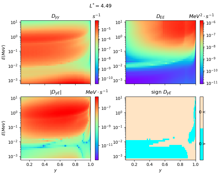
Due to the multi-scale, localized and highly asymmetric physical processes involved in radiation belt dynamics, the local diffusion frame expressed in (y,E)(y,E) is spatially inhomogeneous and presents high levels of anisotropy as shown in Figure 6 for DD taken at L∗=4.49L^{*}=4.49. The 2D tensor anisotropy ratio is also represented in Figure 7.

∂f∂t=1G∇⋅(G    D       ∇f)\frac{\partial f}{\partial t}=\frac{1}{G}\nabla\cdot(G\hbox to9.39pt{\vbox to9.62pt{\pgfpicture\makeatletter\hbox{\hskip 4.69374pt\lower-3.41666pt\hbox to0.0pt{\lxSVG@begingroup@{_scopebegin} \lxSVG@begingroup@{stroke} \lxSVG@begingroup@{fill} \lxSVG@setlinewidth{\the\pgflinewidth}\lxSVG@begingroup@{stroke-width} \lx@inpgf@ignorespaces\nullfont\hbox to0.0pt{\lxSVG@begingroup@{_scopebegin} { {{}}\lx@inpgf@ignorespaces\hbox{\hbox{{\lxSVG@begingroup@{_scopebegin} {{}{}{{ {}{}}}{ {}{}} {{}{{\lx@inpgf@ignorespaces}}}{{}{\lx@inpgf@ignorespaces}}{}{{}{\lx@inpgf@ignorespaces}} {\lx@inpgf@ignorespaces }{{{{\lx@inpgf@ignorespaces}}\lxSVG@begingroup@{_scopebegin} \lxSVG@transformcm{1.0}{0.0}{0.0}{1.0}{-4.27847pt}{-3.41666pt}\lxSVG@begingroup@{transform} \pgfsys@hbox{58}\lxSVG@closescope }}} \lxSVG@closescope }}} { {}}{}{\lx@inpgf@ignorespaces}{}{{}}{}{{}}{}{\lx@inpgf@ignorespaces} {}{}{ {}}{}{\lx@inpgf@ignorespaces}{}{{}}{}{{}}{}{\lx@inpgf@ignorespaces} {}{}\lxSVG@begingroup@{_scopebegin} \lxSVG@setlinewidth{\the\pgflinewidth}\lxSVG@begingroup@{stroke-width} \lx@inpgf@ignorespaces\lxSVG@roundcap\lxSVG@begingroup@{stroke-linecap} \lx@inpgf@ignorespaces{}\lxSVG@stroke\lxSVG@drawpath@unclipped{M -6.2 6.49 L 6.2 6.49 M -6.2 8.28 L 6.2 8.28}{fill:none} \lx@inpgf@ignorespaces \lxSVG@closescope } \lxSVG@closescope {{ {}{}{}}}{\lx@inpgf@ignorespaces}{\lx@inpgf@ignorespaces}\hss}\lxSVG@discardpath\lxSVG@closescope \hss}}\lxSVG@closescope\endpgfpicture}}\nabla f) (30)

with

    D       =(Dy​yDy​EDy​EDE​E)\hbox to9.39pt{\vbox to9.62pt{\pgfpicture\makeatletter\hbox{\hskip 4.69374pt\lower-3.41666pt\hbox to0.0pt{\lxSVG@begingroup@{_scopebegin} \lxSVG@begingroup@{stroke} \lxSVG@begingroup@{fill} \lxSVG@setlinewidth{\the\pgflinewidth}\lxSVG@begingroup@{stroke-width} \lx@inpgf@ignorespaces\nullfont\hbox to0.0pt{\lxSVG@begingroup@{_scopebegin} { {{}}\lx@inpgf@ignorespaces\hbox{\hbox{{\lxSVG@begingroup@{_scopebegin} {{}{}{{ {}{}}}{ {}{}} {{}{{\lx@inpgf@ignorespaces}}}{{}{\lx@inpgf@ignorespaces}}{}{{}{\lx@inpgf@ignorespaces}} {\lx@inpgf@ignorespaces }{{{{\lx@inpgf@ignorespaces}}\lxSVG@begingroup@{_scopebegin} \lxSVG@transformcm{1.0}{0.0}{0.0}{1.0}{-4.27847pt}{-3.41666pt}\lxSVG@begingroup@{transform} \pgfsys@hbox{58}\lxSVG@closescope }}} \lxSVG@closescope }}} { {}}{}{\lx@inpgf@ignorespaces}{}{{}}{}{{}}{}{\lx@inpgf@ignorespaces} {}{}{ {}}{}{\lx@inpgf@ignorespaces}{}{{}}{}{{}}{}{\lx@inpgf@ignorespaces} {}{}\lxSVG@begingroup@{_scopebegin} \lxSVG@setlinewidth{\the\pgflinewidth}\lxSVG@begingroup@{stroke-width} \lx@inpgf@ignorespaces\lxSVG@roundcap\lxSVG@begingroup@{stroke-linecap} \lx@inpgf@ignorespaces{}\lxSVG@stroke\lxSVG@drawpath@unclipped{M -6.2 6.49 L 6.2 6.49 M -6.2 8.28 L 6.2 8.28}{fill:none} \lx@inpgf@ignorespaces \lxSVG@closescope } \lxSVG@closescope {{ {}{}{}}}{\lx@inpgf@ignorespaces}{\lx@inpgf@ignorespaces}\hss}\lxSVG@discardpath\lxSVG@closescope \hss}}\lxSVG@closescope\endpgfpicture}}=\begin{pmatrix}D_{yy}&D_{yE}\\ D_{yE}&D_{EE}\end{pmatrix} (31)

and GG the Jacobian of the transformation from the canonical space to (y,E)(y,E).

Refer to caption
Figure 6: 2D mapping of the diffusion tensor terms Dy​yD_{yy}, DE​ED_{EE} and Dy​ED_{yE}, taken at L∗=4.49L^{*}=4.49.
Refer to caption
Figure 7: Ratio of anisotropy of the diffusion tensor taken at L∗=4.49L^{*}=4.49.

Based on this diffusion model, the radiation belt study community implemented several physical codes like the pioneering ONERA’s Salammbô code [3, 26, 35], the British Antarctic Survey (BAS) Radiation Belt model code [27], the Storm-Time Evolution of Electron Radiation Belt (STEERB) code [24] and the Versatile Electron Radiation Belt (VERB) code [23]. Cumulative improvements in the modelling of physical processes occurring in the inner magnetosphere led to more and more accurate depictions of the radiation belt dynamics by these codes, especially during the main phases of geomagnetic events. However, their finite difference based numerical resolution started to show its limit to tackle all the induced numerical challenges [4, 5].

Recently, a transition to a finite volume based resolution was initiated in the Salammbô code. This was motivated by the suitability of the FV method for diffusion equations and to take advantage of the conservativity property. In order to cope with the high levels of anisotropy and take into account the tricky cross diffusion terms Dy​ED_{yE} without numerical artefacts, the use of nonlinear finite volume schemes seemed inevitable. Thus, NLPTFA and NLMPFA schemes were adapted and tested over the tricky pitch angle and energy diffusion (30), with the results reported in [4].

In this section, we test the R-NLMPFA in the radiation belt context and we focus on its computational cost, which is compared to NLTPFA and NLMPFA. We consider the transient diffusion problem (30) evaluated over Tsimu=90000​sT_{\rm simu}=90000s. We adopt the 2D diffusion tensor DD evaluated at the plan L∗=4.49L^{*}=4.49 and showed in Figure 6. Note that the diffusion coefficients were derived from estimations of resonant particle–particle interactions wave–particle (using the WAPI code [36]).

We start with the initial state finit=1030f_{\rm init}=10^{30} and we impose the boundary conditions presented in Table 7.

The Picard algorithm is initialized with the output of a linear FV scheme, cleaned from overshoots and undershoots, and we adopt the residual (27), more adapted to the high dispersion of the solution. We also fix a maximum number of nonlinear iterations Niter,max=300N_{\rm iter,\rm max}=300, and we consider that the Picard algorithm did not converge above that number. We report in Table 8 the extremum values of ff, the average number of Picard iterations per time iteration Niter,avgN_{\rm iter,\rm avg}, the percentage of time iterations where the Picard algorithm did not converge (Niter>300N_{\rm iter}>300).

Table 7: Boundary conditions adopted for the transient simulation.
Boundary location Boundary condition type Explanation
ymin=0.0867y_{\rm min}=0.0867 f=0f=0 Absence of trapped particles at the atmosphere
ymax=1.0y_{\rm max}=1.0 ∂f∂y=0\frac{\partial f}{\partial y}=0 Equatorial symmetry
Emin=5.664⋅10−4​M​e​VE_{\rm min}=5.664\cdot 10^{-4}~MeV f=1030​M​e​V−1​s−3f=10^{30}~MeV^{-1}s^{-3} Low energy seeding
Emax=12.561​M​e​VE_{\rm max}=12.561~MeV f=0f=0 Limit of magnetic trapping at very high energy
Table 8: Transient simulation results with the NLTPFA,NLMPFA and R-NLMPFA schemes for different Δ​t\Delta t, at Tsimu=90000​sT_{\rm simu}=90000s.
Scheme Δ​t\Delta t 100​s100s 1000​s1000s 10000​s10000s
NLTPFA fminf_{\rm min} 3.96⋅10263.96\cdot 10^{26} 4.05⋅10264.05\cdot 10^{26} 4.97⋅10264.97\cdot 10^{26}
fmaxf_{\rm max} 1.000001191⋅10301.000001191\cdot 10^{30} 1.000000448⋅10301.000000448\cdot 10^{30} 9.99⋅10299.99\cdot 10^{29}
Niter,avgN_{\rm iter,\rm avg} 11 11 22
NLMPFA fminf_{\rm min} 3.95⋅10263.95\cdot 10^{26} 4.06⋅10264.06\cdot 10^{26} 4.96⋅10264.96\cdot 10^{26}
fmaxf_{\rm max} 9.99⋅10269.99\cdot 10^{26} 9.99⋅10269.99\cdot 10^{26} 9.99⋅10299.99\cdot 10^{29}
Niter,avgN_{\rm iter,\rm avg} 1.231.23 7.957.95 242.66242.66
%no−conv\%_{\rm no-conv} 00 00 66.66%66.66\%
R-NLMPFA fminf_{\rm min} 4.12⋅10264.12\cdot 10^{26} 4.34⋅10264.34\cdot 10^{26} 5.18⋅10265.18\cdot 10^{26}
fmaxf_{\rm max} 9.99⋅10299.99\cdot 10^{29} 9.99⋅10299.99\cdot 10^{29} 9.99⋅10299.99\cdot 10^{29}
Niter,avgN_{\rm iter,\rm avg} 11 1.011.01 3.113.11

For all the time steps Δ​t\Delta t we tested, the NLPTFA scheme showed the least Niter,avgN_{\rm iter,\rm avg} values (at maximum 2 Picard iterations per time iteration), followed very closely by the R-NLMPFA (at maximum 4 Picard iterations per time iteration). Hence, the transition from a only positivity preserving scheme to a full monotonicity preserving scheme in our application does not sensibly increase the computational cost. Focusing on the two schemes that also preserve extremum values, the R-NLMPFA prevails with much lower Niter,avgN_{\rm iter,\rm avg} values than the NLMPFA schemes. Most notably, we did not observe with R-NLMPFA any oscillating profiles in the residuals, contrary to those observed with the NLMPFA scheme (see Figure 8). This annoying behavior, frequently reported with the NLMPFA scheme, is mainly reponsible for the non-convergence of the Picard algorithm at some time iterations. The R-NLMPFA very likely avoids their occurrence due to its relaxed linearized stencil.

00505010010015015020020025025030030035035010−710^{-7}10−710^{-7}10−610^{-6}10−510^{-5}10−410^{-4}10−310^{-3}Iteration numberResidueNLTPFANLMPFAR-NLMPFA
Figure 8: Residuals at each Picard iteration step, at n×Δ​t=70000​sn\times\Delta t=70000s for Δ​t=10000​s\Delta t=10000s

6 Conclusion

We presented in this paper the construction of a new nonlinear finite volume scheme, R-NLMPFA, adapted to highly anisotropic diffusion equations. This scheme shares the convex combination structure adopted by typical nonlinear FV schemes and a cell-centered formulation. However, it stands out with its monotonicity preserving property obtained by a set of conditions less restrictive than those needed for an M-matrix construction. This construction leads to a full monotonicity preserving scheme, i.e., a positivity and minimum-maximum principle preserving scheme, in addition to a larger linearized stencil over Cartesian grids. Adimensionnal numerical tests involving diffusion tensors with very high anisotropy ratios showed an important reduction of the computational cost with the R-NLMPFA, especially when compared to the analogous extremum preserving scheme NLMPFA. These results were also confirmed on the numerically challenging radiation belts application. The next step consists in generalizing the construction of the R-NLMPFA to three dimensions and/or quadrilateral meshes, which seems achievable since the monotonicity conditions at the core of the construction are still valid for these types of mesh.

Acknowledgments

This research was supported by CNES – The French Space Agency, ONERA – The French Aerospace Lab, and the University of Monash.

Appendix A Construction of NLTPFA and NLMPFA convex combination weights

The NLTPFA scheme construction is based on the forms (9) of F1F_{1} and F2F_{2}. Injecting these expressions in (5) gives

FK,σ=αK,L​fK−βK,L​fL−(μ1​a1​(f)−μ2​a2​(f))F_{K,\sigma}=\alpha_{K,L}f_{K}-\beta_{K,L}f_{L}-(\mu_{1}a_{1}(f)-\mu_{2}a_{2}(f)) (32)

with a1,a2>0a_{1},a_{2}>0 containing the edge unknowns, responsible for the loss of the MM-matrix structure. The expression μ1​a1−μ2​a2\mu_{1}a_{1}-\mu_{2}a_{2} is annihilated by imposing μ1​a1−μ2​a2=0\mu_{1}a_{1}-\mu_{2}a_{2}=0 and μ1+μ2=1\mu_{1}+\mu_{2}=1, which yields

{μ1=a2a1+a2 and μ2=a1a1+a2 if ​a1+a2≠0,μ1=μ2=12 otherwise.\left\{\begin{array}[]{ll}\mu_{1}=\frac{a_{2}}{a_{1}+a_{2}}\quad\mbox{ and }\quad\mu_{2}=\frac{a_{1}}{a_{1}+a_{2}}&\quad\text{ if }a_{1}+a_{2}\neq 0,\\ \mu_{1}=\mu_{2}=\frac{1}{2}&\quad\text{ otherwise}.\end{array}\right.

The NLMPFA scheme construction, on the other hand, is based on the cell-centered form of F1F_{1} and F2F_{2} as reported in the equation (10), which can be framed in the following general form (with the same notation as in subsection 3.2 – so MM and NN are chosen accordingly to the signs of Dx​y​(K)D_{xy}(K) and Dx​y​(L)D_{xy}(L))

F1=λ1​(fK−fL)+ν1​(fK−fM)⏟G1′ and F2=−λ2​(fL−fK)−ν2​(fL−fN)⏟G2′.F_{1}=\lambda_{1}(f_{K}-f_{L})+\underbrace{\nu_{1}(f_{K}-f_{M})}_{G_{1}^{\prime}}\quad\mbox{ and }\quad F_{2}=-\lambda_{2}(f_{L}-f_{K})-\underbrace{\nu_{2}(f_{L}-f_{N})}_{G_{2}^{\prime}}.

Injecting these expressions in (5) yields

FK,σ=(μ1​λ1+μ2​λ2)​(fK−fL)+[μ1​G1′−μ2​G2′].F_{K,\sigma}=(\mu_{1}\lambda_{1}+\mu_{2}\lambda_{2})(f_{K}-f_{L})+[\mu_{1}G_{1}^{\prime}-\mu_{2}G_{2}^{\prime}]. (33)

The NLMPFA scheme aims to recast the latter flux expression in the multi-point form (12), by discarding the transverse flux branch G2′G_{2}^{\prime} responsible for the loss of the MM-matrix structure. Thus, μ1,μ2\mu_{1},\mu_{2} are chosen to either annihilate the bracketed expression in the last equation, or express it in a form that is appropriate to the LMP structure:

{μ1=|G2′||G1′|+|G2′| and μ2=|G1′||G1′|+|G2′| if ​G1′+G2′≠0,μ1=μ2=12 otherwise.\begin{gathered}\left\{\begin{array}[]{ll}\mu_{1}=\frac{|G_{2}^{\prime}|}{|G_{1}^{\prime}|+|G_{2}^{\prime}|}\quad\mbox{ and }\quad\mu_{2}=\frac{|G_{1}^{\prime}|}{|G_{1}^{\prime}|+|G_{2}^{\prime}|}&\quad\mbox{ if }G_{1}^{\prime}+G_{2}^{\prime}\neq 0,\\[6.99997pt] \mu_{1}=\mu_{2}=\frac{1}{2}&\quad\text{ otherwise}.\end{array}\right.\end{gathered}

In other words:

  • •

    if G1′​G2′≥0G_{1}^{\prime}G_{2}^{\prime}\geq 0 then G1′​|G2′|=|G1′|​G2′G_{1}^{\prime}|G_{2}^{\prime}|=|G_{1}^{\prime}|G_{2}^{\prime} and thus

    FK,σ=(μ1​λ1+μ2​λ2)​(fK−fL).F_{K,\sigma}=(\mu_{1}\lambda_{1}+\mu_{2}\lambda_{2})(f_{K}-f_{L}).
  • •

    if G1′​G2′<0G_{1}^{\prime}G_{2}^{\prime}<0 then |G1′|​G2′=−G1′​|G2′||G_{1}^{\prime}|G_{2}^{\prime}=-G_{1}^{\prime}|G_{2}^{\prime}| and thus

    FK,σ=(μ1​λ1+μ2​λ2)​(fK−fL)+2​μ1​G1′=(μ1​λ1+μ2​λ2)​(fK−fL)+2​μ1​ν1​(fK−fMK).F_{K,\sigma}=(\mu_{1}\lambda_{1}+\mu_{2}\lambda_{2})(f_{K}-f_{L})+2\mu_{1}G_{1}^{\prime}=(\mu_{1}\lambda_{1}+\mu_{2}\lambda_{2})(f_{K}-f_{L})+2\mu_{1}\nu_{1}(f_{K}-f_{M_{K}}).

Appendix B Choice of the weights c1,c2c_{1},c_{2} to ensure the monotonicity conditions

To present a choice of c1c_{1} and c2c_{2} in Section 3.2 that ensures Conditions (A0)–(A3), we use the notations in Figure 9.

cK​(i,j)c_{K}(i,j)σ1\sigma_{1}σ2\sigma_{2}σ3\sigma_{3}σ4\sigma_{4}𝒆𝒙\boldsymbol{e_{x}}𝒆𝒚\boldsymbol{e_{y}}
Figure 9: edge notations on a cell KK.

For each p∈{1,2,3,4}p\in\{1,2,3,4\}, following (18)–(19) the flux FK,σpF_{K,\sigma_{p}} is expressed, with obvious notations, as

FK,σp={(μ1σp​λ1σp+μ2σp​λ2σp)​(fK−fLσp)+c1σp​μ1σp​ν1σp​(fK−fMσp)+c2σp​μ2σp​ν2σp​(fNσp−fLσp) if ​G1σp​G2σp≥0,(μ1σp​λ1σp+μ2σp​λ2σp)​(fK−fLσp)+(2−c1σp)​μ1σp​ν1σp​(fK−fMσp)+c2σp​μ2σp​ν2σp​(fNσp−fLσp) if ​G1σp​G2σp<0.F_{K,\sigma_{p}}=\left\{\begin{array}[]{l@{\ }l}\begin{array}[]{l}\displaystyle(\mu_{1}^{\sigma_{p}}\lambda_{1}^{\sigma_{p}}+\mu_{2}^{\sigma_{p}}\lambda_{2}^{\sigma_{p}})(f_{K}-f_{L^{\sigma_{p}}})\\ \quad\displaystyle+c_{1}^{\sigma_{p}}\mu_{1}^{\sigma_{p}}\nu_{1}^{\sigma_{p}}(f_{K}-f_{M^{\sigma_{p}}})+c_{2}^{\sigma_{p}}\mu_{2}^{\sigma_{p}}\nu_{2}^{\sigma_{p}}(f_{N^{\sigma_{p}}}-f_{L^{\sigma_{p}}})\end{array}&\mbox{ if }G_{1}^{\sigma_{p}}G_{2}^{\sigma_{p}}\geq 0\,,\\[15.00002pt] \begin{array}[]{l}\displaystyle(\mu_{1}^{\sigma_{p}}\lambda_{1}^{\sigma_{p}}+\mu_{2}^{\sigma_{p}}\lambda_{2}^{\sigma_{p}})(f_{K}-f_{L^{\sigma_{p}}})\\ \quad\displaystyle+(2-c_{1}^{\sigma_{p}})\mu_{1}^{\sigma_{p}}\nu_{1}^{\sigma_{p}}(f_{K}-f_{M^{\sigma_{p}}})+c_{2}^{\sigma_{p}}\mu_{2}^{\sigma_{p}}\nu_{2}^{\sigma_{p}}(f_{N^{\sigma_{p}}}-f_{L^{\sigma_{p}}})\end{array}&\mbox{ if }G_{1}^{\sigma_{p}}G_{2}^{\sigma_{p}}<0.\end{array}\right. (34)

We unify the previous expression for more clarity by introducing the parameter θσp\theta^{\sigma_{p}} such that

θσp={c1σp if ​G1σp​G2σp≥02−c1σp if ​G1σp​G2σp<0\theta^{\sigma_{p}}=\left\{\begin{array}[]{ll}c_{1}^{\sigma_{p}}&\text{ if }G_{1}^{\sigma_{p}}G_{2}^{\sigma_{p}}\geq 0\\[5.0pt] 2-c_{1}^{\sigma_{p}}&\text{ if }G_{1}^{\sigma_{p}}G_{2}^{\sigma_{p}}<0\end{array}\right.

Then (34) becomes

FK,σi=(μ1σp​λ1σp+μ2σp​λ2σp)​(fK−fLσp)+θσp​μ1σp​ν1σp​(fK−fMσp)+c2σp​μ2σp​ν2σp​(fNσp−fLσp).F_{K,\sigma_{i}}=(\mu_{1}^{\sigma_{p}}\lambda_{1}^{\sigma_{p}}+\mu_{2}^{\sigma_{p}}\lambda_{2}^{\sigma_{p}})(f_{K}-f_{L^{\sigma_{p}}})+\theta^{\sigma_{p}}\mu_{1}^{\sigma_{p}}\nu_{1}^{\sigma_{p}}(f_{K}-f_{M^{\sigma_{p}}})+c_{2}^{\sigma_{p}}\mu_{2}^{\sigma_{p}}\nu_{2}^{\sigma_{p}}(f_{N^{\sigma_{p}}}-f_{L^{\sigma_{p}}}). (35)

We define a couple (c1,c2)(c_{1},c_{2}) on each discretization direction, i.e., a unique couple for each σp\sigma_{p} is applied on each mesh cell. Thus, we have to determine four pairs of weighing coefficients. Imposing the conservativity property (4) links the coefficients on both sides of each edge:

c1σp=c2σp+2 and c2σp=c1σp+2 for ​p∈1,2.c_{1}^{\sigma_{p}}=c_{2}^{\sigma_{p}+2}\quad\mbox{ and }\quad c_{2}^{\sigma_{p}}=c_{1}^{\sigma_{p}+2}\quad\text{ for }p\in{1,2}. (36)

This reduces the number of weights to be determined to 4, namely (c1σ1,c2σ1,c1σ2,c2σ2)(c_{1}^{\sigma_{1}},c_{2}^{\sigma_{1}},c_{1}^{\sigma_{2}},c_{2}^{\sigma_{2}}).

We then apply the condition (A0), that is m1i,j>0m_{1}^{i,j}>0. From (35) we find

m1i,j=\displaystyle m_{1}^{i,j}={} μ1σ1​λ1σ1+μ2σ1​λ2σ1+θσ1​μ1σ1​ν1σ1+μ1σ2​λ1σ2+μ2σ2​λ2σ2+θσ2​μ1σ2​ν1σ2\displaystyle\mu_{1}^{\sigma_{1}}\lambda_{1}^{\sigma_{1}}+\mu_{2}^{\sigma_{1}}\lambda_{2}^{\sigma_{1}}+\theta^{\sigma_{1}}\mu_{1}^{\sigma_{1}}\nu_{1}^{\sigma_{1}}+\mu_{1}^{\sigma_{2}}\lambda_{1}^{\sigma_{2}}+\mu_{2}^{\sigma_{2}}\lambda_{2}^{\sigma_{2}}+\theta^{\sigma_{2}}\mu_{1}^{\sigma_{2}}\nu_{1}^{\sigma_{2}} (37)
+μ1σ3​λ1σ3+μ2σ3​λ2σ3+θσ3​μ1σ3​ν1σ3+μ1σ4​λ1σ4+μ2σ4​λ2σ4+θσ4​μ1σ4​ν1σ4.\displaystyle+\mu_{1}^{\sigma_{3}}\lambda_{1}^{\sigma_{3}}+\mu_{2}^{\sigma_{3}}\lambda_{2}^{\sigma_{3}}+\theta^{\sigma_{3}}\mu_{1}^{\sigma_{3}}\nu_{1}^{\sigma_{3}}+\mu_{1}^{\sigma_{4}}\lambda_{1}^{\sigma_{4}}+\mu_{2}^{\sigma_{4}}\lambda_{2}^{\sigma_{4}}+\theta^{\sigma_{4}}\mu_{1}^{\sigma_{4}}\nu_{1}^{\sigma_{4}}.

which can be written in the following convinient form

m1i,j=∑r=14(μ1σr​λ1σr+μ2σr​λ2σr+θσr​μ1σr​ν1σr).m_{1}^{i,j}=\sum_{r=1}^{4}\left(\mu_{1}^{\sigma_{r}}\lambda_{1}^{\sigma_{r}}+\mu_{2}^{\sigma_{r}}\lambda_{2}^{\sigma_{r}}+\theta^{\sigma_{r}}\mu_{1}^{\sigma_{r}}\nu_{1}^{\sigma_{r}}\right).

This shows, since all these coefficients are strictly positive by construction, that (A0) is always valid.

We now move to conditions (A1):

m2i,j<0,m4i,j<0,m6i,j<0,m8i,j<0.m_{2}^{i,j}<0\,,\quad m_{4}^{i,j}<0\,,\quad m_{6}^{i,j}<0\,,\quad m_{8}^{i,j}<0.

The expressions of these coefficients depend on the location of MσpM^{\sigma_{p}} in the local cell numbering around the cell KK (see Figure 3), which in turn depends on the sign of Dx​y​(K)D_{xy}(K). To take this into account and later on for (A3)) we define the following parameters

ψ1σp={1​ if ​Dx​y​(K)≥00​ if ​Dx​y​(K)<0\psi_{1}^{\sigma_{p}}=\begin{cases}1\text{ if }D_{xy}(K)\geq 0\\ 0\text{ if }D_{xy}(K)<0\end{cases} (38)

and from (35) we deduce the expressions of m2i,j,m4i,j,m6i,j,m8i,jm_{2}^{i,j},m_{4}^{i,j},m_{6}^{i,j},m_{8}^{i,j}:

m2i,j=\displaystyle m_{2}^{i,j}={} −[μ1σ1​λ1σ1+μ2σ1​λ2σ1+c2σ1​μ2σ1​ν2σ1+ψ1σ2​θσ2​μ1σ2​ν1σ2+(1−ψ1σ4)​θσ4​μ1σ4​ν1σ4],\displaystyle-\left[\mu_{1}^{\sigma_{1}}\lambda_{1}^{\sigma_{1}}+\mu_{2}^{\sigma_{1}}\lambda_{2}^{\sigma_{1}}+c_{2}^{\sigma_{1}}\mu_{2}^{\sigma_{1}}\nu_{2}^{\sigma_{1}}+\psi_{1}^{\sigma_{2}}\theta^{\sigma_{2}}\mu_{1}^{\sigma_{2}}\nu_{1}^{\sigma_{2}}+(1-\psi_{1}^{\sigma_{4}})\theta^{\sigma_{4}}\mu_{1}^{\sigma_{4}}\nu_{1}^{\sigma_{4}}\right], (39)
m4i,j=\displaystyle m_{4}^{i,j}={} −[μ1σ2​λ1σ2+μ2σ2​λ2σ2+c2σ2​μ2σ2​ν2σ2+ψ1σ1​θσ1​μ1σ1​ν1σ1+(1−ψ1σ3)​θσ3​μ1σ3​ν1σ3],\displaystyle-\left[\mu_{1}^{\sigma_{2}}\lambda_{1}^{\sigma_{2}}+\mu_{2}^{\sigma_{2}}\lambda_{2}^{\sigma_{2}}+c_{2}^{\sigma_{2}}\mu_{2}^{\sigma_{2}}\nu_{2}^{\sigma_{2}}+\psi_{1}^{\sigma_{1}}\theta^{\sigma_{1}}\mu_{1}^{\sigma_{1}}\nu_{1}^{\sigma_{1}}+(1-\psi_{1}^{\sigma_{3}})\theta^{\sigma_{3}}\mu_{1}^{\sigma_{3}}\nu_{1}^{\sigma_{3}}\right],
m6i,j=\displaystyle m_{6}^{i,j}={} −[μ1σ3​λ1σ3+μ2σ3​λ2σ3+c2σ3​μ2σ3​ν2σ3+ψ1σ4​θσ4​μ1σ4​ν1σ4+(1−ψ1σ2)​θσ2​μ1σ2​ν1σ2],\displaystyle-\left[\mu_{1}^{\sigma_{3}}\lambda_{1}^{\sigma_{3}}+\mu_{2}^{\sigma_{3}}\lambda_{2}^{\sigma_{3}}+c_{2}^{\sigma_{3}}\mu_{2}^{\sigma_{3}}\nu_{2}^{\sigma_{3}}+\psi_{1}^{\sigma_{4}}\theta^{\sigma_{4}}\mu_{1}^{\sigma_{4}}\nu_{1}^{\sigma_{4}}+(1-\psi_{1}^{\sigma_{2}})\theta^{\sigma_{2}}\mu_{1}^{\sigma_{2}}\nu_{1}^{\sigma_{2}}\right],
m8i,j=\displaystyle m_{8}^{i,j}={} −[μ1σ4​λ1σ4+μ2σ4​λ2σ4+c2σ4​μ2σ4​ν2σ4+ψ1σ3​θσ3​μ1σ3​ν1σ3+(1−ψ1σ1)​θσ1​μ1σ1​ν1σ1].\displaystyle-\left[\mu_{1}^{\sigma_{4}}\lambda_{1}^{\sigma_{4}}+\mu_{2}^{\sigma_{4}}\lambda_{2}^{\sigma_{4}}+c_{2}^{\sigma_{4}}\mu_{2}^{\sigma_{4}}\nu_{2}^{\sigma_{4}}+\psi_{1}^{\sigma_{3}}\theta^{\sigma_{3}}\mu_{1}^{\sigma_{3}}\nu_{1}^{\sigma_{3}}+(1-\psi_{1}^{\sigma_{1}})\theta^{\sigma_{1}}\mu_{1}^{\sigma_{1}}\nu_{1}^{\sigma_{1}}\right].

Similarly as for (A0), the conditions (A1) are then valid for any choice of c1c_{1} and c2c_{2}, since 0<μ1,μ2,c1,c2<10<\mu_{1},\mu_{2},c_{1},c_{2}<1 and ν1,ν2>0\nu_{1},\nu_{2}>0.

Let us now consider (A2), that is, m1i,j+m2i,j+m6i,j>0m_{1}^{i,j}+m_{2}^{i,j}+m_{6}^{i,j}>0 which translates using (35) into

(μ1σ2​λ1σ2+μ2σ2​λ2σ2)+(μ1σ4​λ1σ4+μ2σ4​λ2σ4)+θσ1​μ1σ1​ν1σ1+θσ3​μ1σ3​ν1σ3⏟A−(c2σ1​μ2σ1​ν2σ1+c2σ3​μ2σ3​ν2σ3)⏟B>0.\begin{gathered}\underbrace{(\mu_{1}^{\sigma_{2}}\lambda_{1}^{\sigma_{2}}+\mu_{2}^{\sigma_{2}}\lambda_{2}^{\sigma_{2}})+(\mu_{1}^{\sigma_{4}}\lambda_{1}^{\sigma_{4}}+\mu_{2}^{\sigma_{4}}\lambda_{2}^{\sigma_{4}})+\theta^{\sigma_{1}}\mu_{1}^{\sigma_{1}}\nu_{1}^{\sigma_{1}}+\theta^{\sigma_{3}}\mu_{1}^{\sigma_{3}}\nu_{1}^{\sigma_{3}}}_{A}\\ -\underbrace{(c_{2}^{\sigma_{1}}\mu_{2}^{\sigma_{1}}\nu_{2}^{\sigma_{1}}+c_{2}^{\sigma_{3}}\mu_{2}^{\sigma_{3}}\nu_{2}^{\sigma_{3}})}_{B}>0.\end{gathered}

Since (μ1,μ2)(\mu_{1},\mu_{2}) are the coefficients of a convex combination, and θσp≥0\theta^{\sigma_{p}}\geq 0, we derive the following inequalities over the quantities AA and BB

A≥mini,j⁡(λ1σ2,λ2σ2)+mini,j⁡(λ1σ4,λ2σ4),B≤c2σ1​ν2σ1+c2σ3​ν2σ3≤(c2σ1+c2σ3)​maxi,j⁡(ν2σ1,ν2σ3),\begin{gathered}A\geq\min_{i,j}(\lambda_{1}^{\sigma_{2}},\lambda_{2}^{\sigma_{2}})+\min_{i,j}(\lambda_{1}^{\sigma_{4}},\lambda_{2}^{\sigma_{4}}),\\ B\leq c_{2}^{\sigma_{1}}\nu_{2}^{\sigma_{1}}+c_{2}^{\sigma_{3}}\nu_{2}^{\sigma_{3}}\leq(c_{2}^{\sigma_{1}}+c_{2}^{\sigma_{3}})\max_{i,j}(\nu_{2}^{\sigma_{1}},\nu_{2}^{\sigma_{3}}),\end{gathered}

and we obtain a first condition on (c2σ1,c2σ3)(c_{2}^{\sigma_{1}},c_{2}^{\sigma_{3}}), that is on (c2σ1,c1σ1)(c_{2}^{\sigma_{1}},c_{1}^{\sigma_{1}}) using (36):

c2σ3+c2σ1=c1σ1+c2σ1<mini,j⁡(λ1σ2,λ2OPENσ2)+mini,j⁡(λ1σ4,λ2σ4)CLOSEmaxi,j⁡(ν2σ1,ν2σ3).c_{2}^{\sigma_{3}}+c_{2}^{\sigma_{1}}=c_{1}^{\sigma_{1}}+c_{2}^{\sigma_{1}}<\frac{\min_{i,j}(\lambda_{1}^{\sigma_{2}},\lambda_{2}^{\sigma_{2})}+\min_{i,j}(\lambda_{1}^{\sigma_{4}},\lambda_{2}^{\sigma_{4}})}{{\max_{i,j}}(\nu_{2}^{\sigma_{1}},\nu_{2}^{\sigma_{3}})}. (40)

Let us consider (A3):

m2i,jm4i,j−1−m3i,j−1m1i,j>0,m6i,jm4i,j−1−m5i,j−1m1i,j>0,m6i,jm8i,j+1−m7i,j+1m1i,j>0,m2i,jm8i,j+1−m9i,j+1m1i,j>0.\begin{gathered}m_{2}^{i,j}m_{4}^{i,j-1}-m_{3}^{i,j-1}m_{1}^{i,j}>0\,,\quad m_{6}^{i,j}m_{4}^{i,j-1}-m_{5}^{i,j-1}m_{1}^{i,j}>0\,,\\ m_{6}^{i,j}m_{8}^{i,j+1}-m_{7}^{i,j+1}m_{1}^{i,j}>0\,,\quad m_{2}^{i,j}m_{8}^{i,j+1}-m_{9}^{i,j+1}m_{1}^{i,j}>0.\end{gathered}

The expressions of m3,m5,m7,m9m_{3},m_{5},m_{7},m_{9} depend on the location of MσpM^{\sigma_{p}} and NσpN^{\sigma_{p}} which is defined by the sign of Dx​yD_{xy} on KK and LσpL^{\sigma_{p}}. To take that into account, we define the following parameter:

ψ2σp={1​ if ​Dx​y​(Lσp)≥0,0​ if ​Dx​y​(Lσp)<0,\psi_{2}^{\sigma_{p}}=\begin{cases}1\text{ if }D_{xy}(L^{\sigma_{p}})\geq 0,\\ 0\text{ if }D_{xy}(L^{\sigma_{p}})<0,\end{cases} (41)

and from (35) we deduce the expressions of m3i,j,m5i,j,m7i,j,m9i,jm_{3}^{i,j},m_{5}^{i,j},m_{7}^{i,j},m_{9}^{i,j}:

m3i,j=\displaystyle m_{3}^{i,j}={} (1−ψ2σ1)​c2σ1​μ2σ1​ν2σ1+(1−ψ2σ2)​c2σ2​μ2σ2​ν2σ2,\displaystyle(1-\psi_{2}^{\sigma_{1}})c_{2}^{\sigma_{1}}\mu_{2}^{\sigma_{1}}\nu_{2}^{\sigma_{1}}+(1-\psi_{2}^{\sigma_{2}})c_{2}^{\sigma_{2}}\mu_{2}^{\sigma_{2}}\nu_{2}^{\sigma_{2}},
m5i,j=\displaystyle m_{5}^{i,j}={} ψ2σ2​c2σ2​μ2σ2​ν2σ2+ψ2σ3​c2σ3​μ2σ3​ν2σ3,\displaystyle\psi_{2}^{\sigma_{2}}c_{2}^{\sigma_{2}}\mu_{2}^{\sigma_{2}}\nu_{2}^{\sigma_{2}}+\psi_{2}^{\sigma_{3}}c_{2}^{\sigma_{3}}\mu_{2}^{\sigma_{3}}\nu_{2}^{\sigma_{3}},
m7i,j=\displaystyle m_{7}^{i,j}={} (1−ψ2σ3)​c2σ3​μ2σ3​ν2σ3+(1−ψ2σ4)​c2σ4​μ2σ4​ν2σ4,\displaystyle(1-\psi_{2}^{\sigma_{3}})c_{2}^{\sigma_{3}}\mu_{2}^{\sigma_{3}}\nu_{2}^{\sigma_{3}}+(1-\psi_{2}^{\sigma_{4}})c_{2}^{\sigma_{4}}\mu_{2}^{\sigma_{4}}\nu_{2}^{\sigma_{4}},
m9i,j=\displaystyle m_{9}^{i,j}={} ψ2σ1​c2σ1​μ2σ1​ν2σ1+c2σ4​μ2σ4​ν2σ4.\displaystyle\psi_{2}^{\sigma_{1}}c_{2}^{\sigma_{1}}\mu_{2}^{\sigma_{1}}\nu_{2}^{\sigma_{1}}+c_{2}^{\sigma_{4}}\mu_{2}^{\sigma_{4}}\nu_{2}^{\sigma_{4}}.

Since (μ1,μ2)(\mu_{1},\mu_{2}) are the coefficients of a convex combination, and ψ2σp,θσp≥0\psi_{2}^{\sigma_{p}},\theta^{\sigma_{p}}\geq 0, these relations and (37), (39) yield the following inequalities:

m2i,j​m4i,j−1≥mini,j⁡(λ1σ1,λ2σ1)​mini,j−1⁡(λ1σ2,λ2σ2),m6i,j​m4i,j−1≥mini,j⁡(λ1σ3,λ2σ3)​mini,j−1⁡(λ1σ2,λ2σ2),m6i,j​m8i,j+1≥mini,j⁡(λ1σ3,λ2σ3)​mini,j+1⁡(λ1σ4,λ2σ4),m2i,j​m8i,j+1≥mini,j⁡(λ1σ1,λ2σ1)​mini,j+1⁡(λ1σ4,λ2σ4),m1i,j≤maxi,j⁡(λ1σ1,λ2σ1)+maxi,j⁡(λ1σ2,λ2σ2)+maxi,j⁡(λ1σ3,λ2σ3)+maxi,j⁡(λ1σ4,λ2σ4)+2​(ν1σ1+ν1σ2+ν1σ3+ν1σ4)⏟A′,m3i,j−1≤(c2σ1+c2σ2)​maxi,j−1⁡(ν2σ1,ν2σ2),m5i,j−1≤(c2σ2+c2σ3)​maxi,j−1⁡(ν2σ2,ν2σ3),m7i,j+1≤(c2σ3+c2σ4)​maxi,j+1⁡(ν2σ3,ν2σ4),m9i,j+1≤(c2σ1+c2σ4)​maxi,j+1⁡(ν2σ1,ν2σ4).\begin{gathered}m_{2}^{i,j}m_{4}^{i,j-1}\geq\min_{i,j}(\lambda_{1}^{\sigma_{1}},\lambda_{2}^{\sigma_{1}})\min_{i,j-1}(\lambda_{1}^{\sigma_{2}},\lambda_{2}^{\sigma_{2}}),\\ m_{6}^{i,j}m_{4}^{i,j-1}\geq\min_{i,j}(\lambda_{1}^{\sigma_{3}},\lambda_{2}^{\sigma_{3}})\min_{i,j-1}(\lambda_{1}^{\sigma_{2}},\lambda_{2}^{\sigma_{2}}),\\ m_{6}^{i,j}m_{8}^{i,j+1}\geq\min_{i,j}(\lambda_{1}^{\sigma_{3}},\lambda_{2}^{\sigma_{3}})\min_{i,j+1}(\lambda_{1}^{\sigma_{4}},\lambda_{2}^{\sigma_{4}}),\\ m_{2}^{i,j}m_{8}^{i,j+1}\geq\min_{i,j}(\lambda_{1}^{\sigma_{1}},\lambda_{2}^{\sigma_{1}})\min_{i,j+1}(\lambda_{1}^{\sigma_{4}},\lambda_{2}^{\sigma_{4}}),\\ m_{1}^{i,j}\leq\underbrace{\max_{i,j}(\lambda_{1}^{\sigma_{1}},\lambda_{2}^{\sigma_{1}})+\max_{i,j}(\lambda_{1}^{\sigma_{2}},\lambda_{2}^{\sigma_{2}})+\max_{i,j}(\lambda_{1}^{\sigma_{3}},\lambda_{2}^{\sigma_{3}})+\max_{i,j}(\lambda_{1}^{\sigma_{4}},\lambda_{2}^{\sigma_{4}})+2(\nu_{1}^{\sigma_{1}}+\nu_{1}^{\sigma_{2}}+\nu_{1}^{\sigma_{3}}+\nu_{1}^{\sigma_{4}})}_{A^{\prime}},\\ m_{3}^{i,j-1}\leq(c_{2}^{\sigma_{1}}+c_{2}^{\sigma_{2}})\max_{i,j-1}(\nu_{2}^{\sigma_{1}},\nu_{2}^{\sigma_{2}}),\\ m_{5}^{i,j-1}\leq(c_{2}^{\sigma_{2}}+c_{2}^{\sigma_{3}})\max_{i,j-1}(\nu_{2}^{\sigma_{2}},\nu_{2}^{\sigma_{3}}),\\ m_{7}^{i,j+1}\leq(c_{2}^{\sigma_{3}}+c_{2}^{\sigma_{4}})\max_{i,j+1}(\nu_{2}^{\sigma_{3}},\nu_{2}^{\sigma_{4}}),\\ m_{9}^{i,j+1}\leq(c_{2}^{\sigma_{1}}+c_{2}^{\sigma_{4}})\max_{i,j+1}(\nu_{2}^{\sigma_{1}},\nu_{2}^{\sigma_{4}}).\end{gathered} (42)

This leads to conditions on c2σ1c_{2}^{\sigma_{1}}, c2σ2c_{2}^{\sigma_{2}}, c2σ3c_{2}^{\sigma_{3}} and c2σ4c_{2}^{\sigma_{4}}:

c2σ1+c2σ2<mini,j⁡(λ1σ1,λ2σ1)​mini,j−1⁡(λ1σ2,λ2σ2)maxi,j−1⁡(ν2σ1,ν2σ2)​A′,c2σ2+c2σ3=c2σ2+c1σ1<mini,j⁡(λ1σ3,λ2σ3)​mini,j−1⁡(λ1σ2,λ2σ2)maxi,j−1⁡(ν2σ2,ν2σ3)​A′,c2σ3+c2σ4=c1σ1+c1σ2<mini,j⁡(λ1σ3,λ2σ3)​mini,j+1⁡(λ1σ4,λ2σ4)maxi,j+1⁡(ν2σ3,ν2σ4)​A′,c2σ1+c2σ4=c2σ1+c1σ2<mini,j⁡(λ1σ1,λ2σ1)​mini,j+1⁡(λ1σ4,λ2σ4)maxi,j+1⁡(ν2σ1,ν2σ4)​A′.\begin{gathered}c_{2}^{\sigma_{1}}+c_{2}^{\sigma_{2}}<\frac{\min_{i,j}(\lambda_{1}^{\sigma_{1}},\lambda_{2}^{\sigma_{1}})\min_{i,j-1}(\lambda_{1}^{\sigma_{2}},\lambda_{2}^{\sigma_{2}})}{\max_{i,j-1}(\nu_{2}^{\sigma_{1}},\nu_{2}^{\sigma_{2}})A^{\prime}},\\ c_{2}^{\sigma_{2}}+c_{2}^{\sigma_{3}}=c_{2}^{\sigma_{2}}+c_{1}^{\sigma_{1}}<\frac{\min_{i,j}(\lambda_{1}^{\sigma_{3}},\lambda_{2}^{\sigma_{3}})\min_{i,j-1}(\lambda_{1}^{\sigma_{2}},\lambda_{2}^{\sigma_{2}})}{\max_{i,j-1}(\nu_{2}^{\sigma_{2}},\nu_{2}^{\sigma_{3}})A^{\prime}},\\ c_{2}^{\sigma_{3}}+c_{2}^{\sigma_{4}}=c_{1}^{\sigma_{1}}+c_{1}^{\sigma_{2}}<\frac{\min_{i,j}(\lambda_{1}^{\sigma_{3}},\lambda_{2}^{\sigma_{3}})\min_{i,j+1}(\lambda_{1}^{\sigma_{4}},\lambda_{2}^{\sigma_{4}})}{\max_{i,j+1}(\nu_{2}^{\sigma_{3}},\nu_{2}^{\sigma_{4}})A^{\prime}},\\ c_{2}^{\sigma_{1}}+c_{2}^{\sigma_{4}}=c_{2}^{\sigma_{1}}+c_{1}^{\sigma_{2}}<\frac{\min_{i,j}(\lambda_{1}^{\sigma_{1}},\lambda_{2}^{\sigma_{1}})\min_{i,j+1}(\lambda_{1}^{\sigma_{4}},\lambda_{2}^{\sigma_{4}})}{\max_{i,j+1}(\nu_{2}^{\sigma_{1}},\nu_{2}^{\sigma_{4}})A^{\prime}}.\end{gathered}

Combined with (40), this leads to the five following inequalities to be ensured by c1σ1,c2σ1,c1σ2,c2σ2c_{1}^{\sigma_{1}},c_{2}^{\sigma_{1}},c_{1}^{\sigma_{2}},c_{2}^{\sigma_{2}}

c1σ1+c2σ1<mini,j⁡(λ1σ2,λ2σ2)+mini,j⁡(λ1σ4,λ2σ4)maxi,j⁡(ν2σ1,ν2σ3),c2σ1+c2σ2<mini,j⁡(λ1σ1,λ2σ1)​mini,j−1⁡(λ1σ2,λ2σ2)maxi,j−1⁡(ν2σ1,ν2σ2)​A′,c2σ2+c1σ1<mini,j⁡(λ1σ3,λ2σ3)​mini,j−1⁡(λ1σ2,λ2σ2)maxi,j−1⁡(ν2σ2,ν2σ3)​A′,c1σ1+c1σ2<mini,j⁡(λ1σ3,λ2σ3)​mini,j+1⁡(λ1σ4,λ2σ4)maxi,j+1⁡(ν2σ3,ν2σ4)​A′,c2σ1+c1σ2<mini,j⁡(λ1σ1,λ2σ1)​mini,j+1⁡(λ1σ4,λ2σ4)maxi,j+1⁡(ν2σ1,ν2σ4)​A′.\begin{gathered}c_{1}^{\sigma_{1}}+c_{2}^{\sigma_{1}}<\frac{\min_{i,j}(\lambda_{1}^{\sigma_{2}},\lambda_{2}^{\sigma_{2}})+\min_{i,j}(\lambda_{1}^{\sigma_{4}},\lambda_{2}^{\sigma_{4}})}{\max_{i,j}(\nu_{2}^{\sigma_{1}},\nu_{2}^{\sigma_{3}})},\\ c_{2}^{\sigma_{1}}+c_{2}^{\sigma_{2}}<\frac{\min_{i,j}(\lambda_{1}^{\sigma_{1}},\lambda_{2}^{\sigma_{1}})\min_{i,j-1}(\lambda_{1}^{\sigma_{2}},\lambda_{2}^{\sigma_{2}})}{\max_{i,j-1}(\nu_{2}^{\sigma_{1}},\nu_{2}^{\sigma_{2}})A^{\prime}},\\ c_{2}^{\sigma_{2}}+c_{1}^{\sigma_{1}}<\frac{\min_{i,j}(\lambda_{1}^{\sigma_{3}},\lambda_{2}^{\sigma_{3}})\min_{i,j-1}(\lambda_{1}^{\sigma_{2}},\lambda_{2}^{\sigma_{2}})}{\max_{i,j-1}(\nu_{2}^{\sigma_{2}},\nu_{2}^{\sigma_{3}})A^{\prime}},\\ c_{1}^{\sigma_{1}}+c_{1}^{\sigma_{2}}<\frac{\min_{i,j}(\lambda_{1}^{\sigma_{3}},\lambda_{2}^{\sigma_{3}})\min_{i,j+1}(\lambda_{1}^{\sigma_{4}},\lambda_{2}^{\sigma_{4}})}{\max_{i,j+1}(\nu_{2}^{\sigma_{3}},\nu_{2}^{\sigma_{4}})A^{\prime}},\\ c_{2}^{\sigma_{1}}+c_{1}^{\sigma_{2}}<\frac{\min_{i,j}(\lambda_{1}^{\sigma_{1}},\lambda_{2}^{\sigma_{1}})\min_{i,j+1}(\lambda_{1}^{\sigma_{4}},\lambda_{2}^{\sigma_{4}})}{\max_{i,j+1}(\nu_{2}^{\sigma_{1}},\nu_{2}^{\sigma_{4}})A^{\prime}}.\end{gathered} (43)

References

  • [1] R. Eymard, T. Gallouët, R. Herbin, Finite volume methods, Handbook of numerical analysis 7 (2000) 713–1018.
  • [2] J. Droniou, Finite volume schemes for diffusion equations: introduction to and review of modern methods, Mathematical Models and Methods in Applied Sciences 24 (08) (2014) 1575–1619.
  • [3] A. Varotsou, D. Boscher, S. Bourdarie, R. B. Horne, N. P. Meredith, S. A. Glauert, R. H. Friedel, Three-dimensional test simulations of the outer radiation belt electron dynamics including electron-chorus resonant interactions, Journal of Geophysical Research: Space Physics 113 (A12) (2008).
  • [4] N. Dahmen, F. Rogier, V. Maget, On the modelling of highly anisotropic diffusion for electron radiation belt dynamic codes, Computer Physics Communications 254 (2020) 107342.
  • [5] N. A. Dahmen, Développement d’un nouveau coeur numérique pour le code de calcul salammbô de modélisation des ceintures de radiation terrestres, Ph.D. thesis, Institut Supérieur de l’Aéronautique et de l’Espace (2020).
  • [6] D. S. Kershaw, Differencing of the diffusion equation in Lagrangian hydrodynamic codes, J. Comput. Phys. 39 (2) (1981) 375–395.
  • [7] C. Buet, S. Cordier, On the non existence of monotone linear schema for some linear parabolic equations, C. R. Math. Acad. Sci. Paris 340 (5) (2005) 399–404. doi:10.1016/j.crma.2005.01.020.
    URL https://doi-org.ezproxy.lib.monash.edu.au/10.1016/j.crma.2005.01.020
  • [8] C. Le Potier, Un schéma linéaire vérifiant le principe du maximum pour des opérateurs de diffusion très anisotropes sur des maillages déformés, C. R. Math. Acad. Sci. Paris 347 (1-2) (2009) 105–110. doi:10.1016/j.crma.2008.11.006.
    URL https://doi-org.ezproxy.lib.monash.edu.au/10.1016/j.crma.2008.11.006
  • [9] M. Schneider, D. Gläser, B. Flemisch, R. Helmig, Comparison of finite-volume schemes for diffusion problems, Oil & Gas Science and Technology–Revue d’IFP Energies nouvelles 73 (2018) 82.
  • [10] E. Bertolazzi, G. Manzini, A second-order maximum principle preserving finite volume method for steady convection-diffusion problems, SIAM J. Numer. Anal. 43 (5) (2005) 2172–2199 (electronic).
  • [11] J. Droniou, C. Le Potier, Construction and convergence study of schemes preserving the elliptic local maximum principle, SIAM J. Numer. Anal. 49 (2) (2011) 459–490. doi:10.1137/090770849.
  • [12] Z. Sheng, G. Yuan, The finite volume scheme preserving extremum principle for diffusion equations on polygonal meshes, Journal of Computational Physics 230 (7) (2011) 2588–2604.
  • [13] Z. Sheng, G. Yuan, J. Yue, A nonlinear convex combination in the construction of finite volume scheme satisfying maximum principle, Appl. Numer. Math. 156 (2020) 125–139. doi:10.1016/j.apnum.2020.04.014.
  • [14] C. Le Potier, Correction non linéaire et principe du maximum pour la discrétisation d’opérateurs de diffusion avec des schémas volumes finis centrés sur les mailles, C. R. Math. Acad. Sci. Paris 348 (11-12) (2010) 691–695. doi:10.1016/j.crma.2010.04.017.
    URL http://dx.doi.org/10.1016/j.crma.2010.04.017
  • [15] G. Yuan, Z. Sheng, Monotone finite volume schemes for diffusion equations on polygonal meshes, Journal of computational physics 227 (12) (2008) 6288–6312.
  • [16] C. Le Potier, A nonlinear finite volume scheme satisfying maximum and minimum principles for diffusion operators, Int. J. Finite Vol. 6 (2) (2009) 20.
  • [17] C. Cancès, M. Cathala, C. Le Potier, Monotone correction for generic cell-centered finite volume approximations of anisotropic diffusion equations, Numer. Math. 125 (3) (2013) 387–417.
  • [18] K. Lipnikov, D. Svyatskiy, Y. Vassilevski, Interpolation-free monotone finite volume method for diffusion equations on polygonal meshes, J. Comput. Phys. 228 (3) (2009) 703–716. doi:10.1016/j.jcp.2008.09.031.
    URL http://dx.doi.org/10.1016/j.jcp.2008.09.031
  • [19] K. Lipnikov, D. Svyatskiy, Y. Vassilevski, Minimal stencil finite volume scheme with the discrete maximum principle, Russian J. Numer. Anal. Math. Modelling 27 (4) (2012) 369–385.
  • [20] K. Lipnikov, M. Shashkov, D. Svyatskiy, Y. Vassilevski, Monotone finite volume schemes for diffusion equations on unstructured triangular and shape-regular polygonal meshes, J. Comput. Phys. 227 (1) (2007) 492–512. doi:10.1016/j.jcp.2007.08.008.
    URL http://dx.doi.org/10.1016/j.jcp.2007.08.008
  • [21] L. Agelas, R. Eymard, R. Herbin, A nine-point finite volume scheme for the simulation of diffusion in heterogeneous media, C. R. Math. Acad. Sci. Paris 347 (11-12) (2009) 673–676. doi:10.1016/j.crma.2009.03.013.
  • [22] Z. Sheng, G. Yuan, Construction of nonlinear weighted method for finite volume schemes preserving maximum principle, SIAM J. Sci. Comput. 40 (1) (2018) A607–A628. doi:10.1137/16M1098000.
  • [23] D. Subbotin, Y. Shprits, Three-dimensional modeling of the radiation belts using the versatile electron radiation belt (verb) code, Space Weather 7 (10) (2009).
  • [24] Z. Su, F. Xiao, H. Zheng, S. Wang, Steerb: A three-dimensional code for storm-time evolution of electron radiation belt, Journal of Geophysical Research: Space Physics 115 (A9) (2010).
  • [25] J. M. Nordbotten, I. Aavatsmark, G. Eigestad, Monotonicity of control volume methods, Numerische Mathematik 106 (2) (2007) 255–288.
  • [26] S. Bourdarie, V. Maget, Electron radiation belt data assimilation with an ensemble kalman filter relying on the salammbô code, in: Annales geophysicae, Vol. 30, Copernicus GmbH, 2012, pp. 929–943.
  • [27] S. A. Glauert, R. B. Horne, N. P. Meredith, Three-dimensional electron radiation belt simulations using the bas radiation belt model with new diffusion models for chorus, plasmaspheric hiss, and lightning-generated whistlers, Journal of Geophysical Research: Space Physics 119 (1) (2014) 268–289.
  • [28] C. Le Potier, Schéma volumes finis monotone pour des opérateurs de diffusion fortement anisotropes sur des maillages de triangles non structurés, Comptes Rendus Mathematique 341 (12) (2005) 787–792.
  • [29] C. Cancès, M. Cathala, C. Le Potier, Monotone corrections for generic cell-centered finite volume approximations of anisotropic diffusion equations, Numerische Mathematik 125 (3) (2013) 387–417.
  • [30] A. Berman, R. J. Plemmons, Nonnegative matrices in the mathematical sciences, SIAM, 1994.
  • [31] R. Horne, S. Glauert, N. Meredith, D. Boscher, V. Maget, D. Heynderickx, D. Pitchford, Space weather impacts on satellites and forecasting the earth’s electron radiation belts with spacecast, Space Weather 11 (4) (2013) 169–186.
  • [32] M. Schulz, L. Lanzerotti, Particle diffusion in the radiation belts, phys. chem, Space 7 (1974) 215.
  • [33] J. G. Roederer, H. Zhang, Dynamics of magnetically trapped particles, Springer, 2016.
  • [34] K. Kirby, D. Artis, S. Bushman, M. Butler, R. Conde, S. Cooper, K. Fretz, C. Herrmann, A. Hill, J. Kelley, et al., Radiation belt storm probes—observatory and environments, The Van Allen Probes Mission (2012) 59–125.
  • [35] T. Beutier, D. Boscher, A three-dimensional analysis of the electron radiation belt by the salammbô code, Journal of Geophysical Research: Space Physics 100 (A8) (1995) 14853–14861.
  • [36] A. Sicard-Piet, S. Bourdarie, D. Boscher, Wapi: A new model for the wave particle interaction, 37th COSPAR Scientific Assembly 37 (2008) 2890.