Beyond Neighbourhood-Preserving Transformations for Quantization-Based Unsupervised Hashing
Abstract
An effective unsupervised hashing algorithm leads to compact binary codes preserving the neighborhood structure of data as much as possible. One of the most established schemes for unsupervised hashing is to reduce the dimensionality of data and then find a rigid (neighborhood-preserving) transformation that reduces the quantization error. Although employing rigid transformations is effective, we may not reduce quantization loss to the ultimate limits. As well, reducing dimensionality and quantization loss in two separate steps seems to be sub-optimal. Motivated by these shortcomings, we propose to employ both rigid and non-rigid transformations to reduce quantization error and dimensionality simultaneously. We relax the orthogonality constraint on the projection in a PCA-formulation and regularize this by a quantization term. We show that both the non-rigid projection matrix and rotation matrix contribute towards minimizing quantization loss but in different ways. A scalable nested coordinate descent approach is proposed to optimize this mixed-integer optimization problem. We evaluate the proposed method on five public benchmark datasets providing almost half a million images. Comparative results indicate that the proposed method mostly outperforms state-of-art linear methods and competes with end-to-end deep solutions.
MSC
41A05, 41A10, 65D05, 65D17 \KWDKeyword1, Keyword2, Keyword31 Introduction
Search in big image data is one of the major challenges that has many applications in retrieval, classification and clustering of digital images. A well-established approach toward indexing and searching in mass repositories is hashing that assigns binary codes to data records for fast and efficient access. Hashing has been applied to different problems where fast nearest neighbour search is necessary e.g, large-scale clustering Yunchao Gong et al. 2015.


Hashing algorithms can be categorized in two main sub-groups: data-independent and data-dependent algorithms Wang et al. 2018. The locality sensitive hashing (LSH) Andoni and Indyk 2006 is one of the first representatives in the first group where hash functions are constructed using random projections. Although these methods are faster compared with data-dependent algorithms, their performance is inferior for compact binary codes Paulevé et al. 2010. To address this shortcoming, many data-dependent (or learning-based) hashing algorithms which are divided into supervised and unsupervised methods have been proposed. Supervised hashing methods incorporate label information to learn similarity-preserving binary codes while in unsupervised hashing, which is the focus of this paper the affinity information in the data is used for code learning Weiss et al. 2009.
The main challenge in learning similarity-preserving binary codes is the discrete nature of the optimization problems. To tackle this problem different approaches have been proposed including minimizing quantization loss in Iterative Quantization (ITQ) Gong et al. 2013, Angular Quantization (AQ) Gong et al. 2012, equalizing variance across projections in isotropic hashing (IsoHash) Kong and Li 2012, reconstruction loss in an encoder-decoder architecture like in binary autoencoder (BA) Carreira-Perpinan and Raziperchikolaei 2015, and direct binary code learning in spectral hashing (SH) Weiss et al. 2009 and its sparse version Shao et al. 2012. and more recent developments including Anchor Graph Hashing (AGH) Liu et al. 2011, and Discrete Graph Hashing (DGH) Liu et al. 2014 Large Graph Hashing with Spectral Rotation (LGHSR) Li et al. 2017, Discrete Spectral Hashing (DSH) Hu et al. 2018, and Efficient Spectral Hashing (ESH) Hemati et al. 2020. Other recent works on unsupervised hashing include, Optimal Projection Hashing (OPH) Chu et al. 2019 -Nearest Neighbors Hashing (KNNH) He et al. 2019, and Simultaneous Compression and Quantization (SCQ) Hoang et al. 2020. Although deep learning has been mainly applied to the supervised hashing problem, some unsupervised deep hashing algorithms have recently been proposed. Some recent deep unsupervised hashing algorithms include deep hashing (DH) Liong et al. 2015, Unsupervised Hashing with Binary Deep Neural Network (UHBDNN) Do et al. 2016, Deepbit Lin et al. 2016, and Similarity-Adaptive Deep Hashing (SADH) Shen et al. 2018.
Employing a neighbourhood preserving transformation used in many hashing algorithms. For example in the ITQ, IsoHash, AQ, and OPH a rotation matrix is employed to refine projections. Besides, neighbour preserving transformation has also been used in LGHSR and SCQ to improve the quality of SH relaxed solution and simultaneous projection and quantization of data respectively.
The main issue with binarization is destroying neighbourhood structure of data. Having this in mind, rotation matrices seem to be a good choice for reducing quantization loss as they preserve neighbourhood. Although they are effective, we argue that a single rotation is not powerful enough to minimize the quantization error. Instead, we propose to employ transformations beyond rotation that even corrupt neighbourhood structure of data in favour pushing for quantization. As we will see, such transformation coupled with a rotation leads to high quality binary codes that outperforms state-of-art linear unsupervised hashing methods. Although the proposed idea can be applied to many hashing algorithms that employ a single rotation for reducing quantization error, here we choose to develop this idea on top of ITQ which is very fast and still among competitive hashing methods. In ITQ, the data is projected to lower dimensionality and then the optimal rotation is found such that it minimizes the quantization error in two separate steps.
In our method, we employ a transformation beyond rotation and also resolve the discontinuity in projecting data to lower dimensionality and reduce quantization error. We formulate and optimize our objective function such that in our algorithm:
- 1.
The data is projected and quantized simultaneously. This means unlike many conventional linear unsupervised hashing methods, the projection matrix is contributed towards reducing quantization error.
- 2.
We relax the orthogonality on projection matrix in favor of reducing quantization error even if it corrupts the original neighbourhood. We experiment different matrix norms for achieving this non-rigid transformation.
- 3.
An efficient sequential update scheme is proposed for learning the projection matrix.
The left plot in Fig. 1 shows the histogram of transformed data for a neighbourhood preserving transformation (ITQ) while the right shows the same data transformed by a non-neighbourhood preserving operations using our proposed method Sequential Non-rigid Quantization (SNRQ). Apparently, SNRQ pushes data points more distinctively toward +1 and -1 modes compared with ITQ.
Using extensive quantitative experiments on five public detest and also qualitative results, we show that although our transformation corrupts the neighbourhood of data, the final binary codes obtained using our method, preserve more neighbourhood compared with many other linear hashing methods.
2 Proposed Method
Formulation – In this section, we formulate an optimization problem that follows two objectives. Firstly, it is desirable to jointly learn a projection matrix and minimize the quantization loss of projected data. Secondly, the orthogonality constraint on the projection matrix is relaxed such that we can employ a non-rigid transformation for reducing quantization error. These two objectives together enable non-orthogonal projection matrix to contribute to minimizing quantization loss in a way different from the orthogonal rotation matrix. The first objective is achieved by joining the two well known ITQ steps, namely applying PCA to the data and minimizing quantization loss. Let represents zero-centered data in which is the number of training data points and is the data dimensionality. It is well understood that the projection matrix or principal components of data can be obtained by maximizing the objective function
| (1) |
where is the identity matrix and Tr{} is the trace of a matrix. Here we define as with We would like to minimize the quantization loss of transformed data. To do this, we find an orthogonality relaxed matrix (the relaxed orthogonality constraint on will be formulated later in Eq. 3) and an orthogonal rotation matrix such that the quantization loss of thresholding the transformed data at zero is minimized. This can be formulated as minimizing the following:
| (2) |
where is the corresponding binary representation of . In order to jointly learn the projection matrix and minimize the quantization loss using both non-rigid and rigid , we relax the orthogonality constrain on the projection in PCA formulation and also regularize this by a quantization term which leads to our proposed objective function:
| (3) |
subject to and where and are quantization and rigidness regularization parameters, and finally . Note that in Eq. 3 both and are contributing to minimizing quantization loss, , but in different ways as orthogonality constraint on is smoothed whereas is a pure orthogonal rotation matrix. This is one of the main differences between the proposed method and other existing methods e.g., in contrast to ITQ, IsoHash, AQ, and SCQ.
Optimization – In order to jointly minimize the quantization loss and learn the projection matrix, we need to find , , and in a way to maximize the objective function in Eq. 3. Due to binary constraints on , the optimization is intractable. Hence, inspired by technique used in ITQ paper, we use a coordinate descent approach to optimize the objective function over , , and . To this end, in each step we consider one of the , , and variable and the two other matrices are assumed to be constant.
Fix and , and update : In order to optimize the objective in Eq. 3 with respect to , we easily calculate the derivative with respect to as follow:
| (4) |
Having the gradient w.r.t , we found that the L-BFGS-B optimizer Zhu et al. 1997 obtain a good solution for . However, as each variable should be updated multiple times (while other are fixed) we observed that optimizing for directly is a time-consuming procedure. To mitigate this challenge, in the following we propose a sequential approach for updating . As we will show in experiments, sequential approach achieves comparable performance while reducing training time significantly. In sequential scheme, each time one column of is updated while the rest of columns are considered fixed. First, let’s expand the second term (quantization loss) in Eq. 3:
| (5) | ||||
Now let’s expand the relaxed orthogonality constraint (the third term in Eq. 3):
| (6) | ||||
Using Eqs. 5 and 6 for the second and third terms in Eq. 3, respectively, and defining provides us with the objective function for the case that is variable:
| (7) | ||||
Let’s start formulating the problem such that one column of is considered variable while the remaining columns are constant. To this end, the -th column of that is considered variable is denoted by and all other columns are shown by . In this case, for the first term we receive
| (8) | ||||
Note that here first we used the fact that and then removed as the is scalar. Similarly, if we define the -th row of as and the rest of the rows as , then the second term can be written as
| (9) | |||
For the third term in Eq. 7 we write
| (10) | ||||
As and are scalars, can be removed. Similarly, for the last term we obtain
| (11) | |||
Incorporating Eqs. 8, 9, 10, and 11 into Eq. 7, if we set
| (12) |
then by maximizing the following objective function one can obtain the , -th column of :
| (13) |
To update each column of , i.e, , where we have to find that maximizes Eq. 13. The gradient of objective function (Eq. 13) can be calculated as
| (14) |
Now, we use the L-BFGS-B optimizer to obtain solutions. As we will show in experiments, this sequential learning scheme significantly reduces the training time of the proposed algorithm without sacrificing the quality of binary codes. This efficiency is in part because of simplifying the objective function and also reducing the search space by dividing the problem to sub-problems.
Fix and , and update : In this case, the optimization in Eq. 3 takes the following form:
| (15) |
Having in mind that and are fixed, clearly, minimization of Eq. 15 with respect to is equivalent the maximization of where elements of can be either 1 or -1. As we know from ITQ Gong et al. 2013, the optimal can be calculated as
| (16) |
Fix and , and update : For the case that is variable, maximizing Eq. 3 is equivalent to
| (17) |
This is the Orthogonal Procrustes problem where a rotation matrix is found such that two point sets are aligned with each other. Here, these two point sets are the target binary code matrix and projected data . This problem has closed form solution when is a square orthogonal (rotation) matrix Schönemann 1966 which is
| (18) |
where is the singular value decomposition (SVD) of the by matrix .
In summary, in each iteration, Eq. 16 and Eq. 18 are used to update and , respectively.To update , in each iteration, optimization problems for columns of are solved. After obtaining , and , the binary representation of the data can be obtained . When the direct optimization is used for updating we denote our method Non-rigid Quantization (NRQ) and for the sequential case this denoted by SNRQ. Algorithm 1 summarizes the proposed scheme to update all three matrices method.
Implementation Note – We use eigenvectors of corresponding to largest eigenvalues as initialization of . For , we use the rotation matrix obtained by ITQ as initialization of . Although we will show the algorithm is robust to different values for and , to avoid tuning regularization parameters, we set and for all datasets and experiments. In order to choose , the only consideration is to keep it larger than 1. This can be understood based on Eq. 12 which shows there is a trade-off between reducing quantization error and maximizing variance across projections. This is clear that the quantization error is our priority. The algorithm is fairly robust to , and based on our experiments, any number between to easily does the job. For the number of iterations, experiments on a variety of detests show that 70 iterations are generally sufficient, and after that, the loss function does not change significantly. As a results, We set the number of iterations to 70. An implementation of the proposed method is provided in supplementary material.
Input: Data matrix X, number of iterations
regularization parameters and
Output: Projection matrix , rotation matrix
Initialization: Initialize and
3 Experiments and Results
Datasets and Evaluation protocol The performance of the proposed SNRQ algorithm is evaluated on five standard benchmark datasets, MNIST LeCun et al. 1998, CIFAR-10 Krizhevsky 2009, an unbalanced dataset LabelMe-12-50K Uetz and Behnke 2009, a medical image dataset NCT-CRC-HE-100K Macenko et al. 2009, and a multi-label NUS-WIDE Chua et al. 2009. These datasets provide a total of 489,000 images for learning and testing.
The MNIST dataset contains 70,000 gray-scale images all of size pixels. There are 10 classes in this dataset for handwritten digits.
The CIFAR-10 dataset is a 10-class dataset consisting of 60,000 color images of size pixels.
The LabelMe-12-50K dataset is a 12-class dataset containing 50,000 images of size pixels. This dataset is highly imbalanced such that five classes constitute 91% of all images while there is one class that only contains 0.6% of the samples. The images of this dataset have multiple label values between zero and one. In our experiments, same as previous works that employed this dataset He et al. 2019 for evaluating hashing algorithms, we choose the class of the largest label value as the image label.
The NCT-CRC-HE-100K dataset is 9-class histopathology dataset containing 100,000 non-overlapping image patches from hematoxylin & eosin stained (H&E) images of human colorectal cancer and normal tissue. All images are pixels and color-normalized.
The NUS-WIDE dataset is a multilabel dataset that contains 269,000 images collected from Flickr. This database contains 81 ground-truth concepts.
Hash Code Evaluation To evaluate the performance of the SNRQ, we use standard measures for image retrieval quality assessment. These measures include mean Average Precision (mAP), and precision at samples (e.g., precision@1000). Briefly, mAP measures the overall performance of the retrieval over all classes, whereas precision@ calculates the proportion of true positive over top retrieved samples.
| mAP % | precision % @1000 | |||||
|---|---|---|---|---|---|---|
| Method | 16 bits | 32 bits | 64 bits | 16 bits | 32 bits | 64 bits |
| SH | 32.59 | 33.23 | 30.65 | - | - | - |
| SpH | 31.27 | 36.80 | 41.40 | - | - | - |
| KMH | 31.96 | 37.39 | 41.11 | - | - | - |
| BA | 48.48 | 51.72 | 52.73 | - | - | - - |
| ITQ | 46.37 | 50.59 | 53.69 | 69.67 | 75.13 | 80.45 |
| KNNH | 53.07 | 61.11 | 65.55 | 73.99 | 83.32 | 87.05 |
| SCQ | 62.39 | 74.49 | 72.23 | 79.26 | 88.46 | 88.90 |
| NRQ (Ours) | 71.46 | 69.44 | 72.79 | 84.59 | 85.49 | 87.30 |
| SNRQ (Ours) | 64.70 | 76.98 | 73.48 | 80.00 | 88.53 | 88.27 |
| CIFAR-10 | LabelMe-12-50k | |||||
|---|---|---|---|---|---|---|
| Method | 16 bits | 32 bits | 64 bits | 16 bits | 32 bits | 64 bits |
| SH | 18.31 | 16.54 | 15.78 | 12.60 | 12.59 | 12.24 |
| SpH | 18.82 | 20.93 | 23.40 | 13.59 | 15.10 | 17.03 |
| KMH | 18.68 | 20.82 | 22.87 | 13.36 | 15.47 | 16.58 |
| BA | 25.38 | 26.16 | 27.99 | 16.96 | 18.42 | 20.80 |
| ITQ | 26.82 | 27.38 | 28.73 | 18.06 | 19.40 | 20.73 |
| DGH | 27.73 | 27.44 | 28.01 | 21.45 | 22.74 | 25.41 |
| LGHSR | 27.83 | 25.87 | 22.12 | 21.10 | 23.49 | 23.98 |
| DSH | 27.72 | 25.36 | 22.12 | 24.70 | 23.78 | 24.35 |
| SCQ | 27.52 | 27.42 | 30.34 | 22.89 | 24.95 | 26.50 |
| KNNH | 29.06 | 30.82 | 32.60 | 20.13 | 23.79 | 26.22 |
| NRQ (Ours) | 31.42 | 30.87 | 33.05 | 24.27 | 27.40 | 28.65 |
| SNRQ (Ours) | 30.10 | 31.82 | 33.10 | 25.14 | 26.80 | 28.50 |
Results on MNIST dataset:
Following the setting of He et al. 2019 for MNIST data, each image is presented by a GIST 512-D descriptor, 10% of each class is considered for query set and the remaining data is used as training set. Table 1 shows the results for MNIST in terms of mAP, and precision@1000. Clearly, the NRQ and SNRQ methods provide an improvement over other methods in all cases with only one exception for precision@1000 where the SCQ slightly outperforms SNRQ with less than 0.5% in 64 bit.
Results on CIFAR-10 dataset: For this dataset, following the common setting He et al. 2019; Zhang et al. 2015, we used deep 4096-D features extracted from VGG network Simonyan and Zisserman 2014 and sample 10% of each class as query set and the remaining instances as training set. The left half of Table 2 represents the results for this experiment setting. As it can be seen, NRQ and SNRQ outperform state-of-art namely KNNH He et al. 2019 and SCQ Hoang et al. 2020.
Results on LabelMe-12-50k dataset: As it was pointed out, this dataset is highly imbalanced. To ascertain a fair comparison, we calculate mAP values that are macro averages over all classes. Following the common setting He et al. 2019 we sample 10% of each class to construct the query set, and the remaining data points as training set. Besides, VGG network has been used to extract feature vectors. As Table 2 shows, NRQ and SNRQ are performing better and outperform state-of-art methods with a large gap.
Results on NCT-CRC-HE-100K dataset: For this dataset, we used EfficientNet Tan and Le 2019 pre-trained on ImageNet to extract 1280-D feature vectors from images. We randomly sampled 70,000 images (out of 100K) for training set and the rest of images (30,000) for test. For efficiency, we reduced the feature vector dimensionality to 512 values by the PCA. Table 3 shows that NRQ and SNRQ outperform competitive methods based on mAP and precision@1000 with a significant gap.
| mAP % | precision % @1000 | |||||
|---|---|---|---|---|---|---|
| Method | 16 bits | 32 bits | 64 bits | 16 bits | 32 bits | 64 bits |
| ITQ | 55.8 | 57.8 | 59.5 | 68.8 | 72.6 | 75.4 |
| DGH | 49.85 | 47.24 | 51.61 | 74.08 | 77.14 | 77.05 |
| LGHSR | 55.28 | 47.74 | 38.65 | 75.66 | 78.21 | 77.13 |
| DSH | 58.75 | 45.63 | 37.27 | 76.70 | 78.71 | 77.73 |
| KNNH | 58.02 | 61.47 | 64.28 | 70.27 | 74.91 | 78.16 |
| SCQ | 64.90 | 67.25 | 67.75 | 76.03 | 80.07 | 81.01 |
| NRQ (Ours) | 75.32 | 73.08 | 77.25 | 83.94 | 83.32 | 86.91 |
| SNRQ (Ours) | 68.5 | 75.4 | 78.7 | 80.1 | 84.5 | 87.0 |
Results on NUS-WIDE dataset: For NUS-WIDE experiments, we used the common setup in many hashing papers Liu et al. 2011; Shen et al. 2018. In this setting, images are selected which their labels are among the 21 most frequent labels. This leads to 195,834 images. We randomly sample 2,100 images (100 images from each class) from 195,834 images for the test set and the rest of the images are used for training the hash function and populating the hash table. We used VGG-F network Chatfield et al. 2014 to extract features from images. Results for this experiment are reported in Table 4. The results for other algorithms mainly are directly reported from literature. Shen et al. 2018.
| mAP % | precision % @5000 | |||||
|---|---|---|---|---|---|---|
| Method | 16 bits | 32 bits | 64 bits | 16 bits | 32 bits | 64 bits |
| SH | 44.74 | 42.60 | 42.36 | 59.15 | 54.98 | 54.18 |
| AGH | 49.80 | 47.14 | 44.72 | 70.43 | 70.29 | 69.29 |
| DGH | 54.03 | 52.74 | 49.64 | 71.15 | 71.91 | 70.66 |
| LGHSR | 50.79 | 47.72 | 45.45 | 66.79 | 68.59 | 67.60 |
| ITQ | 53.39 | 54.61 | 55.75 | 65.80 | 68.69 | 70.59 |
| DSH | 49.87 | 47.07 | 45.67 | 68.05 | 68.17 | 67.83 |
| KNNH | 55.12 | 57.53 | 58.61 | 66.77 | 69.83 | 71.07 |
| SCQ | 58.34 | 56.21 | 56.10 | 68.45 | 70.64 | 70.81 |
| NRQ (Ours) | 60.83 | 62.08 | 63.34 | 69.91 | 72.07 | 73.82 |
| SNRQ (Ours) | 61.78 | 62.74 | 62.60 | 70.83 | 72.33 | 73.37 |
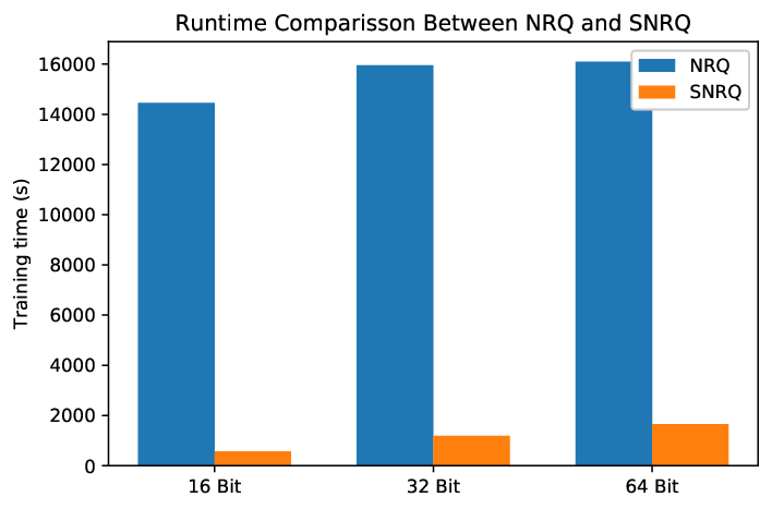


Comparison between NRQ and SNRQ: Here we compare NRQ and SNRQ both in terms of run-time and performance. If we directly update the projection matrix, the training becomes significantly time consuming. To address this, we proposed sequential update scheme which achieves the same performance while significantly reduces the time complexity. The training times of NRQ and SNRQ for CIFAR-10 dataset are shown in Fig. 2. Although based on Fig. 2, SNRQ is significantly faster compared with NRQ, as can be seen from Tables 1, 2, 3, and 4 their performance is similar. The time difference for training may be quite significant for petabyte archives with gigapixel files like satellite imaging and digital pathology where images are commonly quite large, 50,000 by 50,000 pixels. For the latter each patient often comes with many images.
SNRQ vs. ITQ – To validate how employing a non-rigid transformation acts compared with rigid one, we generated a synthetic toy dataset. Fig. 3 shows the transformed data by ITQ and SNRQ on this toy dataset under for values of and . Fig. 3 part (a) represents the toy data. Fig. 3 part (b) shows the same data after transformation by ITQ. Figs. 3 part (c), (d), (e), and (f) show the transformed data using SNRQ for different values of and . This graph reveals role of these regularization parameters in SNRQ algorithm which is controlling the trade-off between preserving neighbourhood structure of data and pushing data points. They can cause unsafe quantization. The smaller the (larger the ) the unsafer the quantization. The quantization loss is increasingly reduced by corrupting neighbourhood.
Comparison of SNRQ with deep unsupervised hashing algorithms – Recently deep learning has been applied to unsupervised hashing including DH Liong et al. 2015, UHBDNN Do et al. 2016, DeepBit Lin et al. 2016, and SADH Shen et al. 2018. To compare SNRQ with Deep unsupervised hashing methods, we employ NUS-WIDE in the setting same as Table 4. As Table 5 shows, SNRQ outperforms UHBDNN and DeepBit by a considerable gap. Compared with SADH, results are highly competitive. Considering DeepBit and SADH are feeding images into a CNN and learn the features, which implies that the quality of features used in SADH, and DeepBit are expectedly better than VGG-F extracted features, it is quite impressive that SNRQ is superior or delivering on par results.
| mAP % | precision % @5000 | |||||
|---|---|---|---|---|---|---|
| Method | 16 bits | 32 bits | 64 bits | 16 bits | 32 bits | 64 bits |
| V+UHBDN | 54.26 | 51.72 | 54.74 | 70.18 | 69.60 | 72.74 |
| R+DeepBit | 39.22 | 40.32 | 42.06 | 45.54 | 51.34 | 57.72 |
| R+SADH | 60.14 | 57.99 | 56.33 | 71.45 | 73.88 | 75.04 |
| V+SNRQ | 61.78 | 62.74 | 62.60 | 70.83 | 72.33 | 73.37 |
Ablation study – We set and for all experiments and datasets. Based on the following experiments, although and regulates the trade-off between preserving the neighbourhood structure and the quality of quantization, SNRQ is robust to changes. Results in Table 6 show the SNRQ performance on MNIST and LabelMe-12-50k datasets for different values , and for the 16 bit setting. Even the worst performance after changing is still state-of-art. We also tested the robustness of SNRQ to changes in . We should not use as it removes the from objective. For , first the value is set to 0.01, then we evaluated SNRQ for 2, 3, 4 and 5 in Table 6. The performance for 2,3, 4 and 5 is consistently high reaching highest for . Considering the proposed objective function in Eq. 3, if we put , there will be no quantization step, and the problem becomes a PCA-like objective function where the orthogonality constraint has been smoothed. Similar to PCA, this would lead to poor binary representations due to accumulated quantization error. For , the projection matrix becomes too dominant and destroys the neighbourhood of data leading to loss of information. Besides, from an optimization point of view, for and , the objective function would become a quadratic function where, given the fact that covariance matrix is positive semi-definite, the maximization is unbounded. As a result, and do not make sense in the context of this paper.
Achieving non-rigid projections – We achieved a non-rigid transformation by relaxing orthogonality constraint on projection matrix. We used the well-known soft orthogonality (SO) . However, there are other ways of achieving this non-rigid projection matrix Bansal et al. 2018. We also tried double soft orthogonality (DSO) , and Mutual Coherence (MC) where we resorted to auto differentiation for implementation. Based on Table 7, the simple soft orthogonality (SO) is achieving better performance in most cases.
| 16 bits, | ||||
| Dataset | ||||
| MNIST | 64.70 | 64.29 | 67.17 | 66.38 |
| LabelMe | 26.08 | 25.29 | 25.29 | 25.10 |
| 16 bits, | ||||
| Dataset | ||||
| MNIST | 63.3 | 63.18 | 65.58 | 65.30 |
| LabelMe | 24.20 | 24.54 | 25.73 | 25.63 |
| mAP % | precision % @1000 | |||||
|---|---|---|---|---|---|---|
| Method | 16 bits | 32 bits | 64 bits | 16 bits | 32 bits | 64 bits |
| SO | 71.34 | 76.83 | 76.57 | 82.94 | 86.13 | 86.30 |
| DSO | 71.07 | 76.29 | 75.40 | 81.59 | 85.60 | 86.16 |
| MC | 72.43 | 73.94 | 76.86 | 82.70 | 83.72 | 85.86 |
4 Conclusions
We introduced Sequential Non-rigid Quantization (SNRQ). The backbone of SNRQ is based on ITQ (iterative quantization) Gong et al. 2013. Although the ideas presented in ITQ are interesting, we argued that learning projection and rotation in two separate steps could be sub-optimal. Furthermore, a rigid transformation may not be enough for reducing quantization to the ultimate limit. Motivated by these limitations, we proposed an algorithm to reduce both dimensionality and quantization loss simultaneously. We also employed a non-rigid transformation to push for quantization beyond rotation. Employing non-rigid transformations is generally against intuition. It does not preserve the neighborhood of data (and all these efforts for reducing quantization error is to preserve more neighborhood after binarization). However, we showed that corrupting neighborhood in favor of reducing quantization eventually leads to better codes. An efficient nested coordinate descent algorithm was employed to update all three matrices. The results on five public datasets totaling almost half a million images showed that the proposed method outperforms the state-of-art linear hashing methods.
As the future work, we plan to extend the idea of binary representation learning using the rigid and non-rigid transformations to the deep architectures. In this framework, while the non-rigid transformations can be realized using regularization terms similar to the soft orthogonality in Eq. 3. For the rigid transformation, one can project the gradient on to orthogonal feasible set using the projection operation proposed in Manton 2002 to update the rotation matrix. Besides, it has been recently demonstrated that hashing can be used in the network quantization task Gholami et al. 2021. This would be interesting to see how the proposed quantization method performs for network quantization.
References
- Andoni and Indyk (2006) Andoni, A., Indyk, P., 2006. Near-optimal hashing algorithms for approximate nearest neighbor in high dimensions, in: 2006 47th Annual IEEE Symposium on Foundations of Computer Science (FOCS’06), pp. 459–468. doi:10.1109/FOCS.2006.49.
- Bansal et al. (2018) Bansal, N., Chen, X., Wang, Z., 2018. Can we gain more from orthogonality regularizations in training deep networks?, in: Advances in Neural Information Processing Systems, pp. 4261–4271.
- Carreira-Perpinan and Raziperchikolaei (2015) Carreira-Perpinan, M.A., Raziperchikolaei, R., 2015. Hashing with binary autoencoders, in: Proceedings of the IEEE Conference on Computer Vision and Pattern Recognition (CVPR).
- Chatfield et al. (2014) Chatfield, K., Simonyan, K., Vedaldi, A., Zisserman, A., 2014. Return of the devil in the details: Delving deep into convolutional nets, in: Proceedings of the British Machine Vision Conference, BMVA Press. doi:http://dx.doi.org/10.5244/C.28.6.
- Chu et al. (2019) Chu, C., Gong, D., Chen, K., Guo, Y., Han, J., Ding, G., 2019. Optimized projection for hashing. Pattern Recognition Letters 117, 169–178.
- Chua et al. (2009) Chua, T.S., Tang, J., Hong, R., Li, H., Luo, Z., Zheng, Y., 2009. Nus-wide: a real-world web image database from national university of singapore, in: Proceedings of the ACM international conference on image and video retrieval, pp. 1–9.
- Do et al. (2016) Do, T.T., Doan, A.D., Cheung, N.M., 2016. Learning to hash with binary deep neural network, in: European Conference on Computer Vision, Springer. pp. 219–234.
- Gholami et al. (2021) Gholami, A., Kim, S., Dong, Z., Yao, Z., Mahoney, M.W., Keutzer, K., 2021. A survey of quantization methods for efficient neural network inference. arXiv preprint arXiv:2103.13630 .
- Gong et al. (2012) Gong, Y., Kumar, S., Verma, V., Lazebnik, S., 2012. Angular quantization-based binary codes for fast similarity search, in: Advances in neural information processing systems, pp. 1196–1204.
- Gong et al. (2013) Gong, Y., Lazebnik, S., Gordo, A., Perronnin, F., 2013. Iterative quantization: A procrustean approach to learning binary codes for large-scale image retrieval. IEEE Transactions on Pattern Analysis and Machine Intelligence 35, 2916–2929. doi:10.1109/TPAMI.2012.193.
- He et al. (2013) He, K., Wen, F., Sun, J., 2013. K-means hashing: An affinity-preserving quantization method for learning binary compact codes, in: Proceedings of the IEEE Conference on Computer Vision and Pattern Recognition (CVPR).
- He et al. (2019) He, X., Wang, P., Cheng, J., 2019. K-nearest neighbors hashing, in: The IEEE Conference on Computer Vision and Pattern Recognition (CVPR).
- Hemati et al. (2020) Hemati, S., Mehdizavareh, M.H., Chenouri, S., Tizhoosh, H.R., 2020. A non-alternating graph hashing algorithm for large scale image search. arXiv preprint arXiv:2012.13138 .
- Heo et al. (2012) Heo, J.P., Lee, Y., He, J., Chang, S.F., Yoon, S.E., 2012. Spherical hashing, in: 2012 IEEE Conference on Computer Vision and Pattern Recognition, pp. 2957–2964. doi:10.1109/CVPR.2012.6248024.
- Hoang et al. (2020) Hoang, T., Do, T.T., Le, H., Le-Tan, D.K., Cheung, N.M., 2020. Simultaneous compression and quantization: A joint approach for efficient unsupervised hashing. Computer Vision and Image Understanding 191, 102852.
- Hu et al. (2018) Hu, D., Nie, F., Li, X., 2018. Discrete spectral hashing for efficient similarity retrieval. IEEE Transactions on Image Processing 28, 1080–1091.
- Kong and Li (2012) Kong, W., Li, W.j., 2012. Isotropic hashing, in: Pereira, F., Burges, C.J.C., Bottou, L., Weinberger, K.Q. (Eds.), Advances in Neural Information Processing Systems, Curran Associates, Inc.
- Krizhevsky (2009) Krizhevsky, A., 2009. Learning multiple layers of features from tiny images , 32–33.
- LeCun et al. (1998) LeCun, Y., Bottou, L., Bengio, Y., Haffner, P., 1998. Gradient-based learning applied to document recognition. Proceedings of the IEEE 86, 2278–2324.
- Li et al. (2017) Li, X., Hu, D., Nie, F., 2017. Large graph hashing with spectral rotation, in: Thirty-First AAAI Conference on Artificial Intelligence.
- Lin et al. (2016) Lin, K., Lu, J., Chen, C.S., Zhou, J., 2016. Learning compact binary descriptors with unsupervised deep neural networks, in: Proceedings of the IEEE Conference on Computer Vision and Pattern Recognition, pp. 1183–1192.
- Liong et al. (2015) Liong, V.E., Lu, J., Wang, G., Moulin, P., Zhou, J., 2015. Deep hashing for compact binary codes learning, in: 2015 IEEE Conference on Computer Vision and Pattern Recognition (CVPR), pp. 2475–2483. doi:10.1109/CVPR.2015.7298862.
- Liu et al. (2014) Liu, W., Mu, C., Kumar, S., Chang, S.F., 2014. Discrete graph hashing, in: Ghahramani, Z., Welling, M., Cortes, C., Lawrence, N., Weinberger, K.Q. (Eds.), Advances in Neural Information Processing Systems, Curran Associates, Inc.
- Liu et al. (2011) Liu, W., Wang, J., Kumar, S., Chang, S.F., 2011. Hashing with graphs, in: Icml.
- Macenko et al. (2009) Macenko, M., Niethammer, M., Marron, J.S., Borland, D., Woosley, J.T., Guan, X., Schmitt, C., Thomas, N.E., 2009. A method for normalizing histology slides for quantitative analysis, in: 2009 IEEE International Symposium on Biomedical Imaging: From Nano to Macro, IEEE. pp. 1107–1110.
- Manton (2002) Manton, J.H., 2002. Optimization algorithms exploiting unitary constraints. IEEE Transactions on Signal Processing 50, 635–650.
- Paulevé et al. (2010) Paulevé, L., Jégou, H., Amsaleg, L., 2010. Locality sensitive hashing: a comparison of hash function types and querying mechanisms. Pattern Recognition Letters 31, 1348–1358.
- Schönemann (1966) Schönemann, P.H., 1966. A generalized solution of the orthogonal procrustes problem. Psychometrika 31, 1–10.
- Shao et al. (2012) Shao, J., Wu, F., Ouyang, C., Zhang, X., 2012. Sparse spectral hashing. Pattern Recognition Letters 33, 271–277. doi:https://doi.org/10.1016/j.patrec.2011.10.018.
- Shen et al. (2018) Shen, F., Xu, Y., Liu, L., Yang, Y., Huang, Z., Shen, H.T., 2018. Unsupervised deep hashing with similarity-adaptive and discrete optimization. IEEE Transactions on Pattern Analysis and Machine Intelligence 40, 3034–3044. doi:10.1109/TPAMI.2018.2789887.
- Simonyan and Zisserman (2014) Simonyan, K., Zisserman, A., 2014. Very deep convolutional networks for large-scale image recognition. arXiv preprint arXiv:1409.1556 .
- Tan and Le (2019) Tan, M., Le, Q.V., 2019. Efficientnet: Rethinking model scaling for convolutional neural networks. arXiv preprint arXiv:1905.11946 .
- Uetz and Behnke (2009) Uetz, R., Behnke, S., 2009. Large-scale object recognition with cuda-accelerated hierarchical neural networks, in: 2009 IEEE international conference on intelligent computing and intelligent systems, IEEE. pp. 536–541.
- Wang et al. (2018) Wang, J., Zhang, T., song, j., Sebe, N., Shen, H.T., 2018. A survey on learning to hash. IEEE Transactions on Pattern Analysis and Machine Intelligence 40, 769–790. doi:10.1109/TPAMI.2017.2699960.
- Weiss et al. (2009) Weiss, Y., Torralba, A., Fergus, R., 2009. Spectral hashing, in: Koller, D., Schuurmans, D., Bengio, Y., Bottou, L. (Eds.), Advances in Neural Information Processing Systems, Curran Associates, Inc.
- Yunchao Gong et al. (2015) Yunchao Gong, Pawlowski, M., Fei Yang, Brandy, L., Boundev, L., Fergus, R., 2015. Web scale photo hash clustering on a single machine, in: 2015 IEEE Conference on Computer Vision and Pattern Recognition (CVPR), pp. 19–27.
- Zhang et al. (2015) Zhang, R., Lin, L., Zhang, R., Zuo, W., Zhang, L., 2015. Bit-scalable deep hashing with regularized similarity learning for image retrieval and person re-identification. IEEE Transactions on Image Processing 24, 4766–4779.
- Zhu et al. (1997) Zhu, C., Byrd, R.H., Lu, P., Nocedal, J., 1997. Algorithm 778: L-bfgs-b: Fortran subroutines for large-scale bound-constrained optimization. ACM Transactions on Mathematical Software (TOMS) 23, 550–560.