Exciton Proliferation and Fate of the Topological Mott Insulator in a
Twisted Bilayer Graphene Lattice Model
Abstract
Topological Mott insulator (TMI) with spontaneous time-reversal symmetry breaking and nonzero Chern number has been discovered in a real-space effective model for twisted bilayer graphene (TBG) at 3/4 filling in the strong coupling limit Chen et al. 2021a. However, the finite temperature properties of such a TMI state remain illusive. In this work, employing the state-of-the-art thermal tensor network and the perturbative field-theoretical approaches, we obtain the finite- phase diagram and the dynamical properties of the TBG model. The phase diagram includes the quantum anomalous Hall and charge density wave phases at low , and a Ising transition separating them from the high- symmetric phases. Due to the proliferation of excitons – particle-hole bound states – the transitions take place at a significantly reduced temperature than the mean-field estimation. The exciton phase is accompanied with distinctive experimental signatures in such as charge compressibilities and optical conductivities close to the transition. Our work explains the smearing of the many-electron state topology by proliferating excitons and opens the avenue for controlled many-body investigations on finite-temperature states in the TBG and other quantum moiré systems.
Introduction.— Since the discovery of correlated insulators and superconducting states in the magic-angle twisted bilayer graphene (TBG) Cao et al. 2018a; Cao et al. 2018b, the quantum moiré systems Trambly de Laissardière et al. 2010; Trambly de Laissardière et al. 2012; Bistritzer and MacDonald 2011 become an active playground for experimental and theoretical investigations on exotic phenomena Yankowitz et al. 2019; Lu et al. 2019; Sharpe et al. 2019; Chen et al. 2020; Kerelsky et al. 2019; Tomarken et al. 2019; Xie et al. 2019; Shen et al. 2020; Serlin et al. 2020; Nuckolls et al. 2020; Pierce et al. 2021; Moriyama et al. 2019; Rozen et al. 2021; Saito et al. 2021; Liu et al. 2020; Naik and Jain 2018; Conte et al. 2019; Tang et al. 2020; Xian et al. 2020; Pan et al. 2020; Venkateswarlu et al. 2020; Lu et al. 2020; Zhang et al. 2020; Maity et al. 2021; Zhang et al. 2021; Pan et al. 2021; Zhang et al. 2021a; Li et al. 2021a; Li et al. 2021b; Xie et al. 2021. The intriguing quantum effects in TBG and transition metal dichacogenide (TMD), besides the superconductivity, encompass a wide range including the orbital ferromagnetism Sharpe et al. 2019; Serlin et al. 2020, (emergent) quantum anomalous Hall (QAH) effect Serlin et al. 2020; Nuckolls et al. 2020; Wu et al. 2021; Das et al. 2021; Li et al. 2021a, large (iso)spin entropy and Pomeranchuk effect Saito et al. 2021; Rozen et al. 2021, etc. Such a plethora of quantum states is believed to originate from the interplay of strong electron correlation and fragile band topology Po et al. 2019; Liu et al. 2019a; Po et al. 2018a; Po et al. 2018b; Liu and Dai 2021; Liu et al. 2019b; Liu and Dai 2020a; Bultinck et al. 2020a; Bultinck et al. 2020b; Bernevig et al. 2021a; Song et al. 2021; Bernevig et al. 2021b; Lian et al. 2021; Bernevig et al. 2021c; Xie et al. 2021. Many theoretical models have been put forward to address these interesting phenomena, and among the positive semidefinite Hamiltonians that are proposed Bernevig et al. 2021b; Bultinck et al. 2020a; Kang and Vafek 2019; Zhang et al. 2021b, a real-space effective model by Kang and Vafek (KV) is able to integrate both key ingredients Kang and Vafek 2018; Kang and Vafek 2019. The KV model and its variants have been investigated via quantum Monte Carlo simulations, which showed certain correlated insulating states such as the inter-valley coherent and quantum valley Hall states, etc, are natural ground states at integer fillings and particularly the charge neutral point (CNP) of the TBG systems Xu et al. 2018; Da Liao et al. 2019; Da Liao et al. 2021; Liao et al. 2021.

Away from CNP, density matrix renormalization group (DMRG) simulations upon the KV model revealed that a QAH state can emerge purely from interactions at 3/4 filling Chen et al. 2021a, which constitutes the long-sought-after topological Mott insulator (TMI) Raghu et al. 2008. Along with other scenarios Bultinck et al. 2020b; Liu and Dai 2020b; Lian et al. 2021 that give rise to the Chern insulators at odd fillings, such a bona fide TMI state provides a strong coupling explanation of the observed quantized Hall conductance in experiments Serlin et al. 2020; Nuckolls et al. 2020. Although the ground state with non-trivial topology in the TBG model is known, the low-energy collective excitations and the experimentally relevant finite- phase diagram are still absent. As the QAH state spontaneously breaks time reversal symmetry (TRS), a thermal phase transition is expected to take place between the topological QAH and high- symmetric phase. However, a naive estimate of the transition temperature according to the band gap Chen et al. 2021a — based on the mean field theory — leads to a value of the order of 100 K, higher than the experimental value ( K) by an order of magnitude Sharpe et al. 2019; Serlin et al. 2020. The difference is believed to stem from the intertwinement of electronic interaction and thermal fluctuaions.
To elucidate the thermal melting of the topological phase and the associated phase diagram, we perform accurate finite- many-body calculations with the exponential tensor renormalization group (XTRG) method Chen et al. 2018; Li et al. 2019. XTRG calculations uncover an Ising-type thermal phase transition between the low- QAH phase and the symmetric phase, and a critical temperature reduced by one order of magnitude compared to the mean-field estimation. These observations are further explained by a field-theoretical approach, which unveiled the emergence of a collective mode of a bounded particle-hole pair–exciton. The excitons are found to have a rather flat and low lying dispersion and proliferate as the temperature elevates, playing an essential role in the melting of the low- phase. The proliferation of excitons leads to a modulation of electron-hole correlations in real space. The entire finite- phase diagram including the low- QAH and CDW phases and the intermediate exciton proliferation phase, is accurately mapped out via both XTRG and field-theoretical approaches.
These results extend the understanding of the zero-temperature phase diagram to finite-temperature and dynamical effects of collective excitations Pan et al. 2021; Khalaf et al. 2020, beyond the exactly solvable limits Lian et al. 2021; Bernevig et al. 2021c; Khalaf et al. 2020; Kang and Vafek 2019; Vafek and Kang 2021; Kwan et al. 2021. Distinctive signatures of the exciton proliferation phase are also revealed to bridge the experimentally accessible observables with theoretical understanding.

Real-space TBG model, thermal tensor networks, and field-theoretical approach.— The KV model considered here is described by the interaction-only Hamiltonian
| (1) |
where sets the energy unit ( 40 meV in realistic system Chen et al. 2021a), the cluster charge term counts the numbers of electrons in each hexagon [c.f., Fig. 1(a)], and represents the assisted hopping term with alternating sign [c.f. Fig. 1(b)]. The results of the present work are mainly based on the YC4 geometry with , where the lattice is under periodic/open boundary condition along vertical/horizontal direction [c.f. Fig. 1(d) for a typical YC4 geoemtry]. We focus on the 3/4 filling of the TBG flat bands with projected Coulomb interaction and correspondingly in Eq. (1) this means the electron number with the valley and spin degrees of freedom polarized. Ref. Chen et al. 2021a identified a CDW insulator and a topologically nontrivial QAH insulator in the ground state of the model, separated by a first-order transition at .
Here, we explore the finite- properties of the TBG model with the XTRG method Chen et al. 2018; Li et al. 2019, which constitutes an accurate many-body method at finite temperature, previously applied to simulate frustrated quantum magnets Chen et al. 2019; Li et al. 2020; Li et al. 2021 as well as correlated fermions at both half filling and finite doping Chen et al. 2021b. We retain up to states, which renders the truncation errors down to low- regime.
We also employ the Gaussian state theory and field-theoretical approach to obtain both thermal and dynamical properties. The thermal state is approximated by a Gaussian ansatz, i.e., the optimal mean-field state, where the order parameters (i.e., all the single particle correlation functions) minimizing the free energy can be obtained efficiently via a set of flow equations Shi et al. 2018; Shi et al. 2020. The particle-hole excitation spectrum can be obtained via the fluctuation analysis Guaita et al. 2019, or alternatively the analytic structure of the scattering -matrix, i.e., the renormalized electronic interaction [c.f. the ladder diagram in Fig. 1(e)]. As the temperature increases, the interaction is strongly renormalized, which drastically modifies the self-energy [c.f. the Hartree-Fock-like contribution in Fig. 1(f)] of the single particle Green function. More details on methodologies are presented in the Supplemental Materials (SM) suppl.
Finite-temperature phase diagram.— Fig. 2(a) summarizes our finite- phase diagram, where the low- phases include the CDW and QAH states, and the symmetric phase can be divided into two regimes, with the orange intermediate- one acquring pronounced collective (exciton) excitations and the red high- state being trivial. As we will show below, there is a crossover between the intermediate- and high- regimes, while the intermediate- and low- phases are separated by a second-order phase transition of Ising universality. Moreover, the two low- phases, i.e., the CDW and QAH ones, are separated by a first-order transition extending from the transition point found in previous DMRG study Chen et al. 2021a.
In Fig. 3(a), the specific heat shows pronounced peaks around for , indicating the existence of second-order phase transitions. The lower phase boundaries in Fig. 2(b) are drawn in this way by performing different scans. The crossover line between the intermediate- and high- regime is estimated by collecting the temperature where the curve starts to scale as the high- limit of [c.f. the red dashed line in Fig. 3(a)] suppl.
Melting of the QAH and CDW states.— To detect the QAH phase, we calculate the current correlation, , where is the average of all the next-nearest-neighbor (NNN) currents [c.f. purple dashed arrows in the inset of Fig. 3(b)] inside the selected hexagon in the -th column of the cylinder, and is the -th hexagon to the right of . We find is nearly a constant in inside the QAH state suppl, indicating the existence of a long-range order. For , decays exponentially with . In Fig. 3(b) we show the current correlation at a sufficiently long distance in the QAH state, i.e., versus , which quickly drops and indicates the vanishing of QAH order above the peak . Notably, the mean-field results [depicted as the grey dots] overestimate the transition temperature while the field theoretical calculation including the contribution of exciton to the quasiparticle self-energy, gives rise to closer to the XTRG results, and together they agree with the corresponding temperature scale observed in the TBG experiment on the melting of the QAH order Sharpe et al. 2019; Serlin et al. 2020. By repeating the calculations of for a wide range of , we identify the existence of QAH phase with in the - plane as shown in Fig. 2(d). Following the similar procedure, but using the charge structure factor at , we identify the CDW phase in the left-bottom corner of the - plane, as shown in Fig. 2(c).
Next, we address the universality class of the phase transition by finite-size data collapsing of the current correlation at with . In the vicinity of the critical point, we have , where the scaling function behaves as . As the low- phase breaks (TRS) symmetry, it is natural to expect a 2D Ising universality class. To verify this, the critical exponents and of the order parameter and correlation length, respectively, are used to collapse the finite- data in Fig. 3(c). In the inset of Fig. 3(c), we plotted the versus and identify the critical temperature as the crossing points between curves of different system sizes. This is the at the thermodynamic limit and slightly different from the peak in the specific peak in Fig. 3(a) for one system size. Then we rescale the -axes as and thus see perfect data collapses within the critical regimes in the main panels of Fig. 3 (c).
Electron-hole correlation and exciton proliferation.— As temperature rises above , the excitons proliferate and result in nontrivial features on the charge correlations. As shown in Fig. 1(d) with and , we place a hole at the very center of the lattice, and find electrons exhibit bunching and anti-bunching modulation behaviors as moving away from the hole, evidencing the existence of particle-hole bound states — excitons — in the system. Such peculiar charge correlations can be quantitatively reflected in the electron-hole correlator , with and measured between two sites (“0” and “”) separated by distances [c.f. Fig. 3(d)], which show increasing correlation whose “sign” changes for different distance in the regime , and shows extremum values at an intermediate temperature (around the mean-field transition temperature), at which the excitons can be easily excited since the single-particle gap now roughly equals the thermal energy scale. The electrons and holes at nearest sites belonging to the same sublattice [i.e., connected via as shown in Fig. 1 (d)] attract each other, while at further distance like they repeal, reflecting the strong influence of excitons in the thermal states. As distance further enhances, e.g., , the electron-hole correlations become rather weak, showing that the excitons are indeed quite local. We note that, the charge correlation decays exponentially with distance, and thus the oscillation behavior is not attributed to Friedel oscillations. When the temperature further elevates and goes beyond , even the short-range charge correlations get smeared by strong thermal fluctuations, all correlations decay () at about . Above this crossover temperature, i.e., in the high- regime, specific heat exhibit scaling as illustrated in Fig. 3(a) suppl.
We also study the compressibility by adding a chemical potential term to the KV model suppl. In Fig. 3(d), the compressibility exhibits a steep jump above and keeps an enhanced value inside the exciton regime. This is a direct result of the exciton proliferation above , where the formation of excitons (bosonic bound state) significantly enhanced the compressibility. Such a steep enhancement can be measured in the quantum capacitance and scanning single electron transistor experiments Eisenstein et al. 1992; Wong et al. 2020; Zondiner et al. 2020. In fact, the compressibility enhancement above the correlated insulators (CDW and QAH phases), is qualitatively consistent with the experimental observation at the same filling of TBG Zondiner et al. 2020.
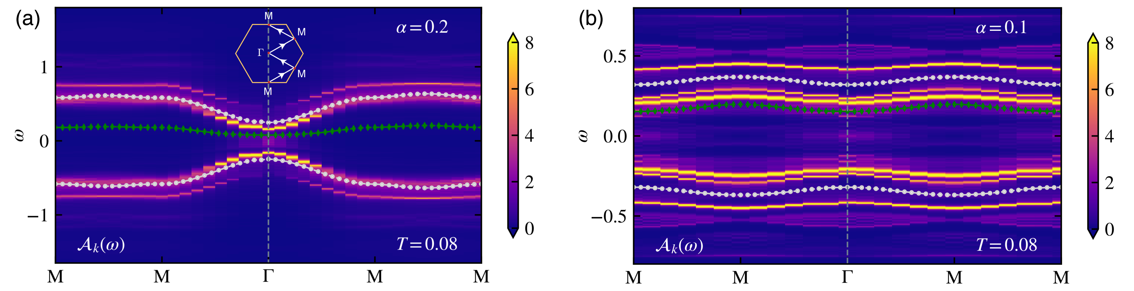
Dynamical signature of excitons.— At the mean-field level, the gap between the conductive and valence bands (white dots in Fig. 4 (a)) in the QAH phase is about (at the point in BZ), giving rise to a transition to the disorder phase at much higher temperature (of the scale of 100 K for realistic materials), at the scale of the ground state band gap Chen et al. 2021a. However, our XTRG computation finds a much lower transition temperature ( 10 K) by one order of magnitude, which agrees with the experimental results Sharpe et al. 2019; Serlin et al. 2020implying the failure of the mean-field theory at finite temperatures.

To explore the mechanism of such low transition temperature, we perform the diagrammatic calculation (see details in SM suppl) on the -matrix in the particle-hole channel and its correction to the self-energy of single-particle Green functions. The poles of the -matrix determine the exciton spectrum. As shown by the green diamonds in Fig. 4 (a) at a representative temperature , the exciton has a much lower energy than the mean-field gap. As a result, at the finite temperature comparable with , many excitons are proliferated by thermal fluctuations, and the scattering with excitons strongly affects single electron behaviors in conductive and valence bands. The effect of excitons to the single particle Green function can be characterized by the -matrix in the Hartree-Fock correction to the self energy (Fig. 1(e) and (f)). In Fig. 4 (a), we show such renormalized spectral function for electrons in conductive and valence bands at , which displays much smaller band gap than that from the mean-field theory. In Fig. 4(b,c), the spectral functions of electrons in the valence band at different temperatures show the reduced quasi-particle weight and the broadened peak as increases. It is remarkable that at the temperature inside the exciton regime, the collective mode assists the valence electron to tunnel across the band gap and redistribute in the positive frequency region. This intriguing feature is the signature of the electron dressed by the cloud of proliferated excitons, which can be probed via spectroscopy. The absorption spectra of probe light display peaks at the exciton frequencies ( GHz shown in Fig. 4). Due to the strong exciton dressing, the current correlation function is thus highly reduced, as shown by the red dots in Fig. 3 (b). Accompanied with the results in Figs. 1 (d) and 3 (d), our results provide a direct observation of proliferated excitations in the 3/4 filling setting of TBG model. We also confirm, a small kinetic term will not qualitatively change the exciton physics observed here suppl.
Discussion.— We extend the studies of the TBG model to the finite-temperature properties and collective excitations. In particular, the excitons formed by a pair of quasi-particle and hole proliferate at intermediate temperatures, which significantly influences the charge correlations and provide a mechanism to melt the QAH phase. We therefore reconcile the large quasi-particle band gap and small QAH transition temperature observed in experiments. The excitons, as collective excitations due to Coulomb interactions, have been investigated and discussed in bilayer graphene Ju et al. 2017; Wu et al. 2017, TBG Kwan et al. 2021; Liu et al. 2017, as well as the recent observation of the QAH in TMD heterobilayers Li et al. 2021a. We note that, the exciton physics here is a distinct feature of flat-band system, different from the Haldane-Hubbard model (see, e.g., Ref. Shao et al. 2021) where the excitons comprised of band electrons and holes do not experience a proliferation upon rising temperature suppl. Our work here shows the emergence of excitons in the strong coupling limit in a TBG lattice model, proposing intriguing exciton physics such as the charge compressibility and the spectral fingerprint in both single-particle and collective models, waiting to be explored in future experiments of quantum moiré systems. We point out that, the valley and spin degrees of freedom, which may give rise to other neutral collective modes (e.g. magnon) and possible Pomeranchuk physics, are omitted in the present model and will be addressed in a future study.
Acknowledgements.
Acknowledgments.— X.Y.L. and B.B.C. contributed equally to this work. X.Y.L., W.L., Z.Y.M. and T.S. are indebted to Jian Kang and Yifan Qu for stimulating discussions. X.Y.L., W.L. and T.S. acknowledge the support from the NSFC through Grant Nos. 11974036, 11834014, 11974363 and 12047503. B.B.C. and Z.Y.M. acknowledge support from the RGC of Hong Kong SAR of China (Grant Nos. 17303019, 17301420, 17301721 and AoE/P-701/20), the Strategic Priority Research Program of the Chinese Academy of Sciences (Grant No. XDB33000000), the K. C. Wong Education Foundation (Grant No. GJTD-2020-01) and the Seed Funding ”Quantum-Inspired explainable-AI” at the HKU-TCL Joint Research Centre for Artificial Intelligence. We thank the High-performance Computing Center at ITP-CAS, the Computational Initiative at the Faculty of Science and Information Technology Service at the University of Hong Kong, and the Tianhe platforms at the National Supercomputer Centers for their technical support and generous allocation of CPU time.References
- Chen et al. (2021a) B.-B. Chen, Y. D. Liao, Z. Chen, O. Vafek, J. Kang, W. Li, and Z. Y. Meng, “Realization of topological Mott insulator in a twisted bilayer graphene lattice model,” Nat Commun 12, 5480 (2021a).
- Cao et al. (2018a) Y. Cao, V. Fatemi, A. Demir, S. Fang, S. L. Tomarken, J. Y. Luo, J. D. Sanchez-Yamagishi, K. Watanabe, T. Taniguchi, E. Kaxiras, R. C. Ashoori, and P. Jarillo-Herrero, “Correlated insulator behaviour at half-filling in magic-angle graphene superlattices,” Nature 556, 80 (2018a).
- Cao et al. (2018b) Y. Cao, V. Fatemi, S. Fang, K. Watanabe, T. Taniguchi, E. Kaxiras, and P. Jarillo-Herrero, “Unconventional superconductivity in magic-angle graphene superlattices,” Nature 556, 43 (2018b).
- Trambly de Laissardière et al. (2010) G. Trambly de Laissardière, D. Mayou, and L. Magaud, “Localization of dirac electrons in rotated graphene bilayers,” Nano Letters 10, 804–808 (2010), pMID: 20121163.
- Trambly de Laissardière et al. (2012) G. Trambly de Laissardière, D. Mayou, and L. Magaud, “Numerical studies of confined states in rotated bilayers of graphene,” Phys. Rev. B 86, 125413 (2012).
- Bistritzer and MacDonald (2011) R. Bistritzer and A. H. MacDonald, “Moiré bands in twisted double-layer graphene,” Proceedings of the National Academy of Sciences 108, 12233–12237 (2011).
- Yankowitz et al. (2019) M. Yankowitz, S. Chen, H. Polshyn, Y. Zhang, K. Watanabe, T. Taniguchi, D. Graf, A. F. Young, and C. R. Dean, “Tuning superconductivity in twisted bilayer graphene,” Science 363, 1059–1064 (2019).
- Lu et al. (2019) X. Lu, P. Stepanov, W. Yang, M. Xie, M. A. Aamir, I. Das, C. Urgell, K. Watanabe, T. Taniguchi, G. Zhang, A. Bachtold, A. H. MacDonald, and D. K. Efetov, “Superconductors, orbital magnets, and correlated states in magic angle bilayer graphene,” Nature 574, 653–657 (2019).
- Sharpe et al. (2019) A. L. Sharpe, E. J. Fox, A. W. Barnard, J. Finney, K. Watanabe, T. Taniguchi, M. A. Kastner, and D. Goldhaber-Gordon, “Emergent ferromagnetism near three-quarters filling in twisted bilayer graphene,” Science 365, 605–608 (2019).
- Chen et al. (2020) G. Chen, A. L. Sharpe, E. J. Fox, Y.-H. Zhang, S. Wang, L. Jiang, B. Lyu, H. Li, K. Watanabe, T. Taniguchi, et al., “Tunable correlated chern insulator and ferromagnetism in a moiré superlattice,” Nature 579, 56–61 (2020).
- Kerelsky et al. (2019) A. Kerelsky, L. J. McGilly, D. M. Kennes, L. Xian, M. Yankowitz, S. Chen, K. Watanabe, T. Taniguchi, J. Hone, C. Dean, et al., “Maximized electron interactions at the magic angle in twisted bilayer graphene,” Nature 572, 95–100 (2019).
- Tomarken et al. (2019) S. L. Tomarken, Y. Cao, A. Demir, K. Watanabe, T. Taniguchi, P. Jarillo-Herrero, and R. C. Ashoori, “Electronic compressibility of magic-angle graphene superlattices,” Phys. Rev. Lett. 123, 046601 (2019).
- Xie et al. (2019) Y. Xie, B. Lian, B. Jäck, X. Liu, C.-L. Chiu, K. Watanabe, T. Taniguchi, B. A. Bernevig, and A. Yazdani, “Spectroscopic signatures of many-body correlations in magic-angle twisted bilayer graphene,” Nature 572, 101–105 (2019).
- Shen et al. (2020) C. Shen, Y. Chu, Q. Wu, N. Li, S. Wang, Y. Zhao, J. Tang, J. Liu, J. Tian, K. Watanabe, T. Taniguchi, R. Yang, Z. Y. Meng, D. Shi, O. V. Yazyev, and G. Zhang, “Correlated states in twisted double bilayer graphene,” Nature Physics (2020), 10.1038/s41567-020-0825-9.
- Serlin et al. (2020) M. Serlin, C. L. Tschirhart, H. Polshyn, Y. Zhang, J. Zhu, K. Watanabe, T. Taniguchi, L. Balents, and A. F. Young, “Intrinsic quantized anomalous Hall effect in a moiré heterostructure,” Science 367, 900–903 (2020).
- Nuckolls et al. (2020) K. P. Nuckolls, M. Oh, D. Wong, B. Lian, K. Watanabe, T. Taniguchi, B. A. Bernevig, and A. Yazdani, “Strongly correlated chern insulators in magic-angle twisted bilayer graphene,” Nature 588, 610–615 (2020).
- Pierce et al. (2021) A. T. Pierce, Y. Xie, J. M. Park, E. Khalaf, S. H. Lee, Y. Cao, D. E. Parker, P. R. Forrester, S. Chen, K. Watanabe, T. Taniguchi, A. Vishwanath, P. Jarillo-Herrero, and A. Yacoby, “Unconventional sequence of correlated chern insulators in magic-angle twisted bilayer graphene,” (2021), arXiv:2101.04123 [cond-mat.mes-hall] .
- Moriyama et al. (2019) S. Moriyama, Y. Morita, K. Komatsu, K. Endo, T. Iwasaki, S. Nakaharai, Y. Noguchi, Y. Wakayama, E. Watanabe, D. Tsuya, K. Watanabe, and T. Taniguchi, “Observation of superconductivity in bilayer graphene/hexagonal boron nitride superlattices,” arXiv e-prints , arXiv:1901.09356 (2019), arXiv:1901.09356 [cond-mat.supr-con] .
- Rozen et al. (2021) A. Rozen, J. M. Park, U. Zondiner, Y. Cao, D. Rodan-Legrain, T. Taniguchi, K. Watanabe, Y. Oreg, A. Stern, E. Berg, P. Jarillo-Herrero, and S. Ilani, “Entropic evidence for a pomeranchuk effect in magic-angle graphene,” Nature 592, 214–219 (2021).
- Saito et al. (2021) Y. Saito, F. Yang, J. Ge, X. Liu, T. Taniguchi, K. Watanabe, J. I. A. Li, E. Berg, and A. F. Young, “Isospin pomeranchuk effect in twisted bilayer graphene,” Nature 592, 220–224 (2021).
- Liu et al. (2020) X. Liu, C.-L. Chiu, J. Y. Lee, G. Farahi, K. Watanabe, T. Taniguchi, A. Vishwanath, and A. Yazdani, “Spectroscopy of a Tunable Moiré System with a Correlated and Topological Flat Band,” arXiv preprint arXiv:2008.07552 (2020).
- Naik and Jain (2018) M. H. Naik and M. Jain, “Ultraflatbands and shear solitons in moiré patterns of twisted bilayer transition metal dichalcogenides,” Phys. Rev. Lett. 121, 266401 (2018).
- Conte et al. (2019) F. Conte, D. Ninno, and G. Cantele, “Electronic properties and interlayer coupling of twisted heterobilayers,” Phys. Rev. B 99, 155429 (2019).
- Tang et al. (2020) Y. Tang, L. Li, T. Li, Y. Xu, S. Liu, K. Barmak, K. Watanabe, T. Taniguchi, A. H. MacDonald, J. Shan, and K. F. Mak, “Simulation of Hubbard model physics in WSe2/WS2 moiré superlattices,” Nature 579, 353–358 (2020).
- Xian et al. (2020) L. Xian, M. Claassen, D. Kiese, M. M. Scherer, S. Trebst, D. M. Kennes, and A. Rubio, “Realization of Nearly Dispersionless Bands with Strong Orbital Anisotropy from Destructive Interference in Twisted Bilayer MoS2,” ArXiv200402964 Cond-Mat (2020), arXiv:2004.02964 [cond-mat] .
- Pan et al. (2020) H. Pan, F. Wu, and S. Das Sarma, “Band topology, Hubbard model, Heisenberg model, and Dzyaloshinskii-Moriya interaction in twisted bilayer ,” Phys. Rev. Research 2, 033087 (2020).
- Venkateswarlu et al. (2020) S. Venkateswarlu, A. Honecker, and G. Trambly de Laissardière, “Electronic localization in twisted bilayer with small rotation angle,” Phys. Rev. B 102, 081103 (2020).
- Lu et al. (2020) Z. Lu, S. Carr, D. T. Larson, and E. Kaxiras, “Lithium intercalation in bilayers and implications for moiré flat bands,” Phys. Rev. B 102, 125424 (2020).
- Zhang et al. (2020) Z. Zhang, Y. Wang, K. Watanabe, T. Taniguchi, K. Ueno, E. Tutuc, and B. J. LeRoy, “Flat bands in twisted bilayer transition metal dichalcogenides,” Nat. Phys. 16, 1093–1096 (2020).
- Maity et al. (2021) I. Maity, P. K. Maiti, H. R. Krishnamurthy, and M. Jain, “Reconstruction of moiré lattices in twisted transition metal dichalcogenide bilayers,” Phys. Rev. B 103, L121102 (2021), arXiv:1912.08702 .
- Zhang et al. (2021) X. Zhang, G. Pan, Y. Zhang, J. Kang, and Z. Y. Meng, “Momentum Space Quantum Monte Carlo on Twisted Bilayer Graphene,” Chinese Physics Letters 38, 077305 (2021).
- Pan et al. (2021) G. Pan, X. Zhang, H. Li, K. Sun, and Z. Y. Meng, “Dynamic properties of collective excitations in twisted bilayer Graphene,” arXiv e-prints , arXiv:2108.12559 (2021), arXiv:2108.12559 [cond-mat.str-el] .
- Zhang et al. (2021a) X. Zhang, K. Sun, H. Li, G. Pan, and Z. Y. Meng, “Superconductivity and bosonic fluid emerging from Moiré flat bands,” arXiv e-prints , arXiv:2111.10018 (2021a), arXiv:2111.10018 [cond-mat.supr-con] .
- Li et al. (2021a) T. Li, S. Jiang, B. Shen, Y. Zhang, L. Li, T. Devakul, K. Watanabe, T. Taniguchi, L. Fu, J. Shan, and K. F. Mak, “Quantum anomalous Hall effect from intertwined moiré bands,” arXiv e-prints , arXiv:2107.01796 (2021a), arXiv:2107.01796 [cond-mat.mes-hall] .
- Li et al. (2021b) H. Li, U. Kumar, K. Sun, and S.-Z. Lin, “Spontaneous fractional Chern insulators in transition metal dichalcogenides Moire superlattices,” arXiv e-prints , arXiv:2101.01258 (2021b), arXiv:2101.01258 [cond-mat.mes-hall] .
- Xie et al. (2021) Y.-M. Xie, C.-P. Zhang, J.-X. Hu, K. F. Mak, and K. T. Law, “Theory of Valley Polarized Quantum Anomalous Hall State in Moiré MoTe2/WSe2 Heterobilayers,” arXiv e-prints , arXiv:2106.13991 (2021), arXiv:2106.13991 [cond-mat.mes-hall] .
- Wu et al. (2021) S. Wu, Z. Zhang, K. Watanabe, T. Taniguchi, and E. Y. Andrei, “Chern insulators, van Hove singularities and topological flat bands in magic-angle twisted bilayer graphene,” Nature Materials 20, 488–494 (2021).
- Das et al. (2021) I. Das, X. Lu, J. Herzog-Arbeitman, Z.-D. Song, K. Watanabe, T. Taniguchi, B. A. Bernevig, and D. K. Efetov, “Symmetry-broken Chern insulators and Rashba-like Landau-level crossings in magic-angle bilayer graphene,” Nature Physics 17, 710–714 (2021).
- Po et al. (2019) H. C. Po, L. Zou, T. Senthil, and A. Vishwanath, “Faithful tight-binding models and fragile topology of magic-angle bilayer graphene,” Phys. Rev. B 99, 195455 (2019).
- Liu et al. (2019a) J. Liu, J. Liu, and X. Dai, “Pseudo Landau level representation of twisted bilayer graphene: Band topology and implications on the correlated insulating phase,” Phys. Rev. B 99, 155415 (2019a).
- Po et al. (2018a) H. C. Po, L. Zou, A. Vishwanath, and T. Senthil, “Origin of Mott insulating behavior and superconductivity in twisted bilayer graphene,” Phys. Rev. X 8, 031089 (2018a).
- Po et al. (2018b) H. C. Po, H. Watanabe, and A. Vishwanath, “Fragile Topology and Wannier Obstructions,” Phys. Rev. Lett. 121, 126402 (2018b).
- Liu and Dai (2021) J. Liu and X. Dai, “Theories for the correlated insulating states and quantum anomalous Hall effect phenomena in twisted bilayer graphene,” Phys. Rev. B 103, 035427 (2021).
- Liu et al. (2019b) J. Liu, Z. Ma, J. Gao, and X. Dai, “Quantum Valley Hall Effect, Orbital Magnetism, and Anomalous Hall Effect in Twisted Multilayer Graphene Systems,” Phys. Rev. X 9, 031021 (2019b).
- Liu and Dai (2020a) J. Liu and X. Dai, “Anomalous Hall effect, magneto-optical properties, and nonlinear optical properties of twisted graphene systems,” npj Computational Materials 6, 57 (2020a).
- Bultinck et al. (2020a) N. Bultinck, E. Khalaf, S. Liu, S. Chatterjee, A. Vishwanath, and M. P. Zaletel, “Ground state and hidden symmetry of magic-angle graphene at even integer filling,” Phys. Rev. X 10, 031034 (2020a).
- Bultinck et al. (2020b) N. Bultinck, S. Chatterjee, and M. P. Zaletel, “Mechanism for Anomalous Hall Ferromagnetism in Twisted Bilayer Graphene,” Phys. Rev. Lett. 124, 166601 (2020b).
- Bernevig et al. (2021a) B. A. Bernevig, Z.-D. Song, N. Regnault, and B. Lian, “Twisted bilayer graphene. I. Matrix elements, approximations, perturbation theory, and a two-band model,” Phys. Rev. B 103, 205411 (2021a).
- Song et al. (2021) Z.-D. Song, B. Lian, N. Regnault, and B. A. Bernevig, “Twisted bilayer graphene. II. Stable symmetry anomaly,” Phys. Rev. B 103, 205412 (2021).
- Bernevig et al. (2021b) B. A. Bernevig, Z.-D. Song, N. Regnault, and B. Lian, “Twisted bilayer graphene. III. Interacting Hamiltonian and exact symmetries,” Phys. Rev. B 103, 205413 (2021b).
- Lian et al. (2021) B. Lian, Z.-D. Song, N. Regnault, D. K. Efetov, A. Yazdani, and B. A. Bernevig, “Twisted bilayer graphene. IV. Exact insulator ground states and phase diagram,” Phys. Rev. B 103, 205414 (2021).
- Bernevig et al. (2021c) B. A. Bernevig, B. Lian, A. Cowsik, F. Xie, N. Regnault, and Z.-D. Song, “Twisted bilayer graphene. V. Exact analytic many-body excitations in Coulomb Hamiltonians: Charge gap, Goldstone modes, and absence of Cooper pairing,” Phys. Rev. B 103, 205415 (2021c).
- Xie et al. (2021) F. Xie, A. Cowsik, Z.-D. Song, B. Lian, B. A. Bernevig, and N. Regnault, “Twisted bilayer graphene. VI. An exact diagonalization study at nonzero integer filling,” Phys. Rev. B 103, 205416 (2021).
- Kang and Vafek (2019) J. Kang and O. Vafek, “Strong coupling phases of partially filled twisted bilayer graphene narrow bands,” Phys. Rev. Lett. 122, 246401 (2019).
- Zhang et al. (2021b) X. Zhang, G. Pan, X. Y. Xu, and Z. Y. Meng, “Sign Problem Finds Its Bounds,” arXiv e-prints , arXiv:2112.06139 (2021b), arXiv:2112.06139 [cond-mat.str-el] .
- Kang and Vafek (2018) J. Kang and O. Vafek, “Symmetry, maximally localized wannier states, and a low-energy model for twisted bilayer graphene narrow bands,” Phys. Rev. X 8, 031088 (2018).
- Xu et al. (2018) X. Y. Xu, K. T. Law, and P. A. Lee, “Kekulé valence bond order in an extended hubbard model on the honeycomb lattice with possible applications to twisted bilayer graphene,” Phys. Rev. B 98, 121406 (2018).
- Da Liao et al. (2019) Y. Da Liao, Z. Y. Meng, and X. Y. Xu, “Valence Bond Orders at Charge Neutrality in a Possible Two-Orbital Extended Hubbard Model for Twisted Bilayer Graphene,” Phys. Rev. Lett. 123, 157601 (2019).
- Da Liao et al. (2021) Y. Da Liao, J. Kang, C. N. Breiø, X. Y. Xu, H.-Q. Wu, B. M. Andersen, R. M. Fernandes, and Z. Y. Meng, “Correlation-induced insulating topological phases at charge neutrality in twisted bilayer graphene,” Phys. Rev. X 11, 011014 (2021).
- Liao et al. (2021) Y.-D. Liao, X.-Y. Xu, Z.-Y. Meng, and J. Kang, “Correlated insulating phases in the twisted bilayer graphene,” Chinese Physics B 30, 017305 (2021).
- Raghu et al. (2008) S. Raghu, X.-L. Qi, C. Honerkamp, and S.-C. Zhang, “Topological Mott Insulators,” Phys. Rev. Lett. 100, 156401 (2008).
- Liu and Dai (2020b) J. Liu and X. Dai, “Anomalous Hall effect, magneto-optical properties, and nonlinear optical properties of twisted graphene systems,” npj Computational Materials 6, 57 (2020b).
- Chen et al. (2018) B.-B. Chen, L. Chen, Z. Chen, W. Li, and A. Weichselbaum, “Exponential thermal tensor network approach for quantum lattice models,” Phys. Rev. X 8, 031082 (2018).
- Li et al. (2019) H. Li, B.-B. Chen, Z. Chen, J. von Delft, A. Weichselbaum, and W. Li, “Thermal tensor renormalization group simulations of square-lattice quantum spin models,” Phys. Rev. B 100, 045110 (2019).
- Khalaf et al. (2020) E. Khalaf, N. Bultinck, A. Vishwanath, and M. P. Zaletel, “Soft modes in magic angle twisted bilayer graphene,” arXiv e-prints , arXiv:2009.14827 (2020), arXiv:2009.14827 [cond-mat.str-el] .
- Vafek and Kang (2021) O. Vafek and J. Kang, “Lattice model for the Coulomb interacting chiral limit of the magic angle twisted bilayer graphene: symmetries, obstructions and excitations,” arXiv e-prints , arXiv:2106.05670 (2021), arXiv:2106.05670 [cond-mat.str-el] .
- Kwan et al. (2021) Y. H. Kwan, Y. Hu, S. H. Simon, and S. A. Parameswaran, “Exciton band topology in spontaneous quantum anomalous hall insulators: Applications to twisted bilayer graphene,” Phys. Rev. Lett. 126, 137601 (2021).
- Eisenstein et al. (1992) J. P. Eisenstein, L. N. Pfeiffer, and K. W. West, “Negative compressibility of interacting two-dimensional electron and quasiparticle gases,” Phys. Rev. Lett. 68, 674–677 (1992).
- Wong et al. (2020) D. Wong, K. P. Nuckolls, M. Oh, B. Lian, Y. Xie, S. Jeon, K. Watanabe, T. Taniguchi, B. A. Bernevig, and A. Yazdani, “Cascade of electronic transitions in magic-angle twisted bilayer graphene,” Nature 582, 198–202 (2020).
- Zondiner et al. (2020) U. Zondiner, A. Rozen, D. Rodan-Legrain, Y. Cao, R. Queiroz, T. Taniguchi, K. Watanabe, Y. Oreg, F. von Oppen, A. Stern, et al., “Cascade of phase transitions and dirac revivals in magic-angle graphene,” Nature 582, 203–208 (2020).
- Chen et al. (2019) L. Chen, D.-W. Qu, H. Li, B.-B. Chen, S.-S. Gong, J. von Delft, A. Weichselbaum, and W. Li, “Two temperature scales in the triangular lattice Heisenberg antiferromagnet,” Phys. Rev. B 99, 140404(R) (2019).
- Li et al. (2020) H. Li, Y. D. Liao, B.-B. Chen, X.-T. Zeng, X.-L. Sheng, Y. Qi, Z. Y. Meng, and W. Li, “Kosterlitz-Thouless melting of magnetic order in the triangular quantum Ising material TmMgGaO4,” Nat. Commun. 11, 1111 (2020).
- Li et al. (2021) H. Li, H.-K. Zhang, J. Wang, H.-Q. Wu, Y. Gao, D.-W. Qu, Z.-X. Liu, S.-S. Gong, and W. Li, “Identification of magnetic interactions and high-field quantum spin liquid in -RuCl3,” Nature Communications 12, 4007 (2021).
- Chen et al. (2021b) B.-B. Chen, C. Chen, Z. Chen, J. Cui, Y. Zhai, A. Weichselbaum, J. von Delft, Z. Y. Meng, and W. Li, “Quantum Many-Body Simulations of the Two-Dimensional Fermi-Hubbard Model in Ultracold Optical Lattices,” Phys. Rev. B 103, L041107 (2021b).
- Shi et al. (2018) T. Shi, E. Demler, and J. Ignacio Cirac, “Variational study of fermionic and bosonic systems with non-gaussian states: Theory and applications,” Annals of Physics 390, 245–302 (2018).
- Shi et al. (2020) T. Shi, E. Demler, and J. I. Cirac, “Variational approach for many-body systems at finite temperature,” Phys. Rev. Lett. 125, 180602 (2020).
- Guaita et al. (2019) T. Guaita, L. Hackl, T. Shi, C. Hubig, E. Demler, and J. I. Cirac, “Gaussian time-dependent variational principle for the bose-hubbard model,” Phys. Rev. B 100, 094529 (2019).
- Ju et al. (2017) L. Ju, L. Wang, T. Cao, T. Taniguchi, K. Watanabe, S. G. Louie, F. Rana, J. Park, J. Hone, F. Wang, and P. L. McEuen, “Tunable excitons in bilayer graphene,” Science 358, 907–910 (2017).
- Wu et al. (2017) F. Wu, T. Lovorn, and A. H. MacDonald, “Topological exciton bands in moiré heterojunctions,” Phys. Rev. Lett. 118, 147401 (2017).
- Liu et al. (2017) X. Liu, K. Watanabe, T. Taniguchi, B. I. Halperin, and P. Kim, “Quantum hall drag of exciton condensate in graphene,” Nature Physics 13, 746–750 (2017).
- Trotter (1959) H. F. Trotter, “On the product of semi-groups of operators,” Proceedings of the American Mathematical Society 10, 545–551 (1959).
- Chen et al. (2017) B.-B. Chen, Y.-J. Liu, Z. Chen, and W. Li, “Series-expansion thermal tensor network approach for quantum lattice models,” Phys. Rev. B 95, 161104 (2017).
- Shao et al. (2021) C. Shao, E. V. Castro, S. Hu, and R. Mondaini, “Interplay of local order and topology in the extended Haldane-Hubbard model,” Phys. Rev. B 103, 035125 (2021).
- Haldane (1988) F. D. M. Haldane, “Model for a Quantum Hall Effect without Landau Levels: Condensed-Matter Realization of the “Parity Anomaly”,” Phys. Rev. Lett. 61, 2015–2018 (1988).
- (85) In Supplementary Materials Sec. I, we briefly summarized exponential tensor renormalization group method, its measurements on thermodynamic quantities, and adaption to fermion systems are introduced. Sec. II is devoted to the details of determination of crossover temperature between intermediate- regime and the high- regime. In Sec. III, we present the current correlation calculations. In Sec. IV, we discuss the thermodynamics of the system in the small- regime. In Sec. V, we present more thermodynamic data for various values. In Sec. VI, we include the electronic compressibility calculations. In Sec. VII and Sec. VIII, the Gaussian state approach and the implementation of perturbative field theoretical calculations on the single-particle and collective excitations are presented. In Sec. IX, we discuss the thermodynamics of Haldane-Hubbard model. The Supplementary Materials include references Chen et al. 2018; Li et al. 2019; Trotter 1959; Chen et al. 2017; Chen et al. 2021a; Shi et al. 2020; Shi et al. 2018; Shao et al. 2021; Haldane 1988.
I Supplemental Materials for
Exciton Proliferation and Fate of the Topological Mott Insulator in a
Twisted Bilayer Graphene Lattice Model
I.1 Section I: Exponential Tensor Renormalization Group Method
As shown in Fig. S1, the main idea of exponential tensor renormalization group (XTRG) Chen et al. 2018; Li et al. 2019 method is, to first construct the initial high-temperature density operator with being an exponentially small inverse temperature, which can be obtained with ease via Trotter-Suzuki decomposition Trotter 1959 or series-expansion methods Chen et al. 2017. Subsequently, we evolve the thermal state exponentially by squaring the density operator iteratively, i.e., . Following this exponential evolution scheme, one can significantly reduce the evolution as well as truncation steps, and thus can obtain highly accurate low- data in greatly improved efficiency.
In XTRG simulations, we compute the internal energy per site
| (S1) |
where is the Hamiltonian [c.f. Eq. (1)] and is the density matrix of the system with sites, and the specific heat via the derivative of internal energy, is
| (S2) |
with the inverse temperature.

When adapting XTRG to fermion systems, one should take care of the fermionic sign of exchanging two electrons. In this work, we are working on the many-body basis , where is the number of electrons at the site and is the vacuum state. Generically in this basis, the one-body operator (assuming ) requires an sign , in addition to transform the state to the state . As shown in Fig. S2, such fermion-sign structure can be encoded in XTRG readily in a matrix product operator with bond dimension .
I.2 Section II: Crossover between exciton proliferation regime and high-T regime
In this section, we will discuss the determination of the crossover between the intermediate- exciton proliferation regime and the high- gas-like regime. In a high temperature (i.e., a small inverse temperature ), the internal energy density of the system
via Taylor expansion, can be expressed as
Thus in the large- limit, it yields
for specific heat.
As shown in Fig. S3, we show the specific heat of a YC412 system at both and , which show predominant power-law decay at high-T regime. As indicated by the red dashed lines in Fig. S3(a,b), we find the high- data asymptotically follow and for and respectively, which are well consistent with the large- limit. We thus determine the crossover temperature between the high- regime and intermediate- regime, by computing the deviation of the specific heat from the high-T behavior, i.e., . To be more specific, we classify those temperatures at which as intermediate-, and otherwise as high-.
I.3 Section III: Detailed current-current correlation calculation
As shown in Fig. S4, we calculate the current-current correlation function , defined in the main text. In a YC412 systems at , establish a plateau over distance , in the quantum anomalous Hall (QAH) region, i.e., for , whereas it decays exponentially for . It means that, the lower- region for the large cases spontaneously break the time-reversal symmetry, manifesting the QAH state. On the other hand, for the small- case ( here), decays exponentially for both regions of and .
I.4 Section IV: More details on the CDW data
In this section, we discuss more detailed thermodynamics results of the CDW phase for . In Fig. S5(a), we show the specific heat curve vs. temperature , which peaks at predominantly, indicating a phase transition there. We also compute the density-density correlation function at various temperatures, with site being fixed at a center site and site running over the lattice. The charge structure factor
| (S3) |
is found to peak at point in the Brillouin zone (BZ). Note there are three pairs of equivalent points in the BZ while only one of them is preferred by the cylindrical geometry, c.f., Ref. Chen et al. 2021a. As shown in Fig. S5(b), for the low- CDW state, the CDW order parameter , structure factor at the point, experiences a sudden drop at the transition temperature upon heating, the same temperature as the specific heat peak locates in Fig. S5(a). Again, the mean-field results overestimate , which is believed to be corrected by the higher-order perturbative calculation towards the XTRG results.
To address the universality class of phase transitions between the CDW phase that breaks -type (discrete translational) symmetries to the symmetric phase at higher temperatures, we follow the same line as in the main text for the current-current correlation , and perform the finite-size data collapsing of in Fig. S5(c). As a function of () and system size , we denote it as . We again using the 2D Ising critical exponents and as the CDW phase breaks symmetry. In the inset of Fig. S5(c), we plotted the versus and identify the critical temperature as the crossing points between curves of different system sizes. The so-estimated is again very closed to the peak of specific heat. Then we rescale the -axes of Fig. S5(c) as and see perfect data collapses within the critical regimes in the main panel of Fig. S5(c).
In Fig. S5(d), we see that the correlation increases rapidly as the long-range anti-bunching correlation melts at the CDW transition temperature. Other than that, we also observe similar particle-hole correlation modulation in the exciton-proliferated intermediate- regime above the CDW phase, as in Fig. 3(d) of the main text. In Fig. S5(d), we also perform the calculation on the compressibility by adding a chemical potential term to the KV model. Similarly, the compressibility exhibits a steep jump above and keeps an enhanced value inside the exciton regime.
I.5 Section V: Detailed -scan for phase diagram
In this section, we will show more results of specific heat , charge structure factor , and the current-current correlation function for various other than and , as complement to the main text. As shown in Fig. S6, in all these cases () the specific heat curves (the first row) clearly show sharp peaks, above which either ( and ) and ( and ) quickly vanish.
I.6 Section VI: Electronic compressibility calculations
In this section, we add a chemical potential term to the original Kang-Vafek model [Eq. (1) in the main text], i.e.
| (S4) |
to account for the electronic response with chemical potential. We calculate the averaged electron density
for different inverse temperature and different chemical potentials ranging from 0 to 0.1. As shown in Fig. S7, for both and , the particle density responds to chemical potential linearly above the transition temperature. The electronic compressibility at is then approximately obtained via,
where is taken. The obtained compressibility versus temperature is shown in Fig. S8 for two cases of and . The results exhibit zero-value compressibility in both QAH and CDW low- phases due to their insulator nature, whereas show finite-value in the intermediate- regime verifying the metallic nature.
I.7 Section VII: Gaussian state approach to twisted bilayer graphene
At finite temperature , the imaginary time evolution equation Shi et al. 2020 for density matrices reads
| (S5) |
which guarantees the monotonic decrease of the free energy with being the free energy operator.
We approximate the density matrix by the Gaussian state
| (S6) |
where is the partition function, is a matrix in the Nambu basis , the creation and annihilation operators and fulfill the anti-commutation relation , and is the number of fermionic modes. The density matrix is fully characterized by its covariance matrix
| (S7) |
By projecting Eq. (S5) in the tangential space of the variational manifold Shi et al. 2018; Shi et al. 2020, we obtain EOM
| (S8) |
where the mean-field free energy is determined by the mean-field Hamiltonian and .
For the Kang-Vafek (KV) model Eq. (1), the diagonal and off-diagonal blocks
| (S9) |
of the mean-field Hamiltonian in the local basis of each hexagon are determined by
| (S10) |
where the six sites in the hexagon are labeled in Fig. S9. The energy per hexagon reads
| (S11) |

The free energy
| (S12) |
decreases monotonically in the imaginary time evolution, where the diagonal matrix is constructed by the eigenvalues of . In the asymptotic limit, the density matrix reaches the thermal equilibrium state, where , and the pairing term due to the repulsive Coulomb interaction inherited by the KV model. As a result, the off-diagonal block .
In agreement with the XTRG approach, the finite-T phase diagram obtained by the optimal mean-field theory consists of the QAH states, the CDW states, and high-T trivial states. It is remarkable that the QAH and CDW states possess a lot of symmetries which are represented by the structure of the covariance matrix . Therefore, the thermal state can be described with very little order parameters, as we will show in the following.
Let us list several typical symmetries of the Hamiltonian. The Hamiltonian has the particle hole symmetry , the time reversal symmetry , the translational symmetry , the rotational symmetry with respect to the center of the hexagon, the reflection symmetry with respect to the horizontal axis , the symmetry of the reflection with respect to the vertical axis and in one sub-lattice. The vectors and axises in the honeycomb Moiré lattice are shown in Fig. S10.

The covariance matrix in the coordinate space shows that the QAH state has symmetries , , and the symmetry . The properties of and the corresponding symmetry are listed as follows:
- •
The particle-hole symmetry .
- •
The translational symmetry The covariance matrices for all hexagons are same, e.g., .
- •
The rotational symmetry , , , , .
- •
The symmetry .
The symmetries play an important role since they completely determine the covariance matrix
| (S13) |
with only three independent order parameters
| (S14) |
where and are the annihilation operators of electrons in sublattices and .
The covariance matrix gives rise to the mean-field Hamiltonian
| (S15) |
in each hexagon through Eq. (S9), with the effective hopping strengths
| (S16) |
between the nearest neighbor, the second-neighbor, and the third-neighbor sites, as shown in Fig. S11.

In the second quantized form, the mean-field Hamiltonian of the honeycomb Moiré lattice reads
| (S17) |
where . The Fourier transforms and result in the mean-field Hamiltonian in the momentum space , where
| (S18) |
is determined by
| (S19) |
The covariance matrix
| (S20) |
can be obtained by the diagonalization of the mean-field Hamiltonian using the unitary transformation , where the Fermi-Dirac distribution is determined by the dispersion relations in the conduction () and valance () bands at the temperature .
The covariance matrix gives rise to the self-consistent equations
| (S21) |
for the order parameters. Close to the phase transition, all the order parameters tend to zero, and Eq. (S21) can be linearized as
| (S22) |
The critical temperature is thus determined by the largest positive eigenvalue of
Furthermore, using symmetries we can significantly reduce the degrees of freedom in the covariance matrix to three order parameters, as a result, the above analysis can be applied to the system in the thermodynamic limit. To speed up the calculation, we first numerically the flow equations of for a small system, and achieve the three order parameters in the thermal state. Using the order parameters of the small system as the initial condition, we solve the non-linear Eq. (S21) to obtain the order parameters for the system in the thermodynamic limit, where the free energy density
| (S23) |
is minimized.
In the CDW phase, the density distribution of the CDW state has three equivalent spatial structures for the system in the thermodynamic limit, which possesses the symmetries , and , respectively. We analyze one of the three equivalent CDW states that maintains the symmetry without loss of generality. The structure of the covariance matrices and in the odd and even rows, respectively, indicates that the CDW state possesses the symmetries , , , and the combination symmetries , . The properties of the covariance matrices and the corresponding symmetry are listed as follows.
- •
The time reversal symmetry and are real symmetric matrices.
- •
The translational symmetry The covariance matrices for each rows are same, e.g., .
- •
The combination symmetry , , .
- •
The combination symmetry , , ; , , ; , , ; , .
- •
The symmetry , .
Therefore, the covariance matrix only has four independent order parameters
| (S24) |
where and are integers. The covariance matrix
| (S25) |
results in the mean-field Hamiltonian
| (S26) |
in odd rows with the hopping strengths
| (S27) |
The combination symmetry determines the relation between the mean-field Hamiltonian in odd and even rows as .
In the second quantized form, the mean-field Hamiltonian of the honeycomb Moiré lattice reads
| (S28) |
The stripe has the translational symmetry and , thus, particles with the momentum hybridize with particles with the momentum and the Brillouin zone shrinks to , which is different from the situation in QAH phases. The Fourier transformation gives rise to the mean-field Hamiltonian in the momentum space , where
| (S29) |
is determined by
| (S30) |
and
| (S31) |
The covariance matrix
| (S32) |
can be obtained by the diagonalization of the mean-field Hamiltonian using the unitary transformation , where the Fermi-Dirac distribution in the CDW phase is determined by the dispersion relation at the temperature .
The covariance matrix leads to the self-consistent equations
| (S33) |
for the order parameters. Close to the phasae transition, all the order parameters tend to zero, and Eq. (S33) can be linearized as
| (S34) |
The critical temperature is determined by the largest positive eigenvalue of the matrix
| (S35) |
Finally, the finite-T phase diagram S12 under the self-consistent mean-field approximation can be obtained, where the first-order transition between the QAH and CDW phases is displayed.
I.8 Section VIII: Exciton spectra and self-energy corrections
At zero temperature, the single-particle Green’s function from the Gaussian state approach (the self-consistent mean-field theory) agrees excellently with the result from DMRG Chen et al. 2021a. With respect to the Gaussian thermal state described by three order parameters in QAH phases, the KV Hamiltonian (S36) is decomposed into normal ordered terms via the Wick theorem as
| (S36) |
where the Fourier transformation is determined by the relative distance and , and we use the Einstein summation convention for the Greek alphabet.

At finite temperature, the two-particle spectrum can be obtained by the ladder diagram approximation beyond the mean-field theory, as shown in Fig. S13, and the self-energy correction, e.g., the Hartree term, becomes
| (S37) |
where the free single-particle Green function . The exciton spectrum can be determined by the density-density correlation function
| (S38) |
It follows from the Heisenberg EOM that
| (S39) |
where
| (S40) |
We define the correlation function in the quasi-particle basis using the transformation . The Fourier transform of EOM (S39) results in
| (S41) |
where the bare density-density correlation function reads
| (S42) |
and the interaction of two quasi-particles is determined by . The spectral decomposition results in
| (S43) |
where the poles of appear in pairs due to the particle-hole symmetry of . It turns out that the lowest band with the dispersion relation corresponds to a collective mode, i.e., the exciton excitation. The bottom of the exciton band is at the -point, and at zero temperature its energy is about for , i.e., one order of magnitude smaller than the bare quasi-particle gap. Additionally, the exciton is robust in the presence of the kinetic energy of the bare electron as illustrated in Fig. S14. The wavefunction of the exciton state in the coordinate space, i.e., the Fourier transformation of , shows that the exciton with the center-of-mass momentum is in the bound state of one electron in the conductive band and one electron in the valence band.
The two-particle correlation function leads to the self-energy correction via Eq. (S37), where is the self-energy
| (S44) |
of the quasi-particle, and is the Bose-Einstein distribution.
We get the Matsubara single-particle Green function with the first-order exciton correction
| (S45) |
In the quasi-particle picture, the single-particle Green function becomes
| (S46) |
where and are the poles and residues of , respectively, which satisfies sum rules and .

The Fock correction to the quasi-particle Green function can also be included as
| (S47) |
where the interaction -matrix is obtained by
| (S48) |
and
| (S49) |
is determined by and .
Finally, the full single-particle Green function including the Hartree-Fock-like corrections becomes
| (S50) |
where and are the poles and residues of the spectral function , respectively. The retarded Green’s function is obtained by the analytic continuation, which determines the spectral function Im. In our numerical calculation, we choose .
Due to the particle-hole symmetry, and we only focus on the valence. Comparing with the spectral function of the free Green function , we find that when the temperature increases, not only the quasi-particle gap is reduced, but the broadened spectral function even has the non-zero distribution at the positive frequency, as shown in Fig. S16. This is a strong evidence of the valence band electron dressed by the excitons. The reduction of the quasi-particle weight and the spectral distribution in the negative frequency domain indicates the decrease of the current-current correlation. As shown in Fig. 3, with the correction of the exciton the current-current correlation decreases much faster than the mean-field result. However, the perturbative expansion fails to predict the correct critical temperature obtained by XTRG. This is because at the higher temperature, many excitons are proliferated, which strongly affect the quasi-particle spectrum as well as the particle-hole spectrum. As a result, the bare Green function in the calculation of the -matrix should be replaced by the exact Green function, namely, the self-consistent calculation of the Green function is required, which will be our future work.


In the CDW phase, the calculation on the -matrix and self-energy corrections can also be performed in the similar way, which also shows the low lying exciton excitation confirmed by the XTRG results.
The Fourier transformation gives rise to the interacting Hamiltonian
| (S51) |
in the momentum space , where the interacting matrix and the permutation matrix .
The two-particle spectrum is also obtained by the ladder diagram approximation. The self-energy correction, e.g., the Hartree term, becomes
| (S52) | ||||
where the free single-particle Green function . The exciton spectrum can be determined by the density-density correlation function
| (S53) | ||||
| (S54) |
It follows from the Heisenberg EOM that
| (S55) |
where
| (S56) | ||||
We define the correlation function in the quasi-particle basis via the transformation in the CDW phase. The Fourier transform of EOM (S55) results in
| (S57) | ||||
| (S58) | ||||
| (S59) |
where the interaction
| (S60) |
of two quasi-particles is determined by and . The spectral decomposition results in
| (S61) |
In the CDW phase, the lowest band with the dispersion relation also corresponds to a collective mode, i.e., the exciton excitation. The lowest energy of the exciton is about 0.15 for , which is smaller then the quasi-particle gap, similar to what happens in the QAH phase. However, the exciton band structure in the CDW phase is significantly distinct from that in the QAH phase due to the different spatial symmetries, as shown in Fig. S17.

The self-energy corrections, i.e., the Hartree-Fock corrections and , can also be obtained in the similar way as Eq. (S44) and Eq. (S47). One only has to change the corresponding quasi-particle Green function and the interaction matrix to those in the CDW phase, which results in the full single-particle Green function
| (S62) |
and the spectral functions . Due to the symmetries mentioned in the last section, there are two degenerate valence bands and two degenerate conductance bands, as a result, four single-particle spectral functions are obtained in the CDW phase. Due to the particle-hole symmetry, we only focus on the spectral function for one of the degenerate valence bands. When the temperature increases, the quasi-particle gap is reduced and the exciton mode assists the valence electron to tunnel across the band gap, as shown in Fig. S18.
Via choosing the specific path in the momentum space, as illustrated in Fig. S19, the difference of the spectral function between the QAH and CDW phases are explicitly displayed. In our case, the period of the spectral function in the CDW phase is reduced by half in the direction. In the QAH phase, the translational symmetry () are preserved. However, the stripe in the CDW phase spontaneously breaks the the translational symmetry () and preserves the translational symmetry (), as a result, the period in the momentum space is reduced.


I.9 Section IX: Numerical results on Haldane-Hubbard model
We perform DMRG () and XTRG () calculations of the spinless Haldane-Hubbard model (HHM) whose Hamiltonian reads
| (S63) |
where and the direction of next-nearest-neighbor (NNN) pair follows the standard Haldane model Haldane 1988, and introduce the nearest-neighbor (NN) repulsion as in, e.g., Ref. Shao et al. 2021. The model in Eq. (S63) keeps the particle-hole symmetry and thus guarantees half filling in the finite-temperature XTRG calculations below. is set as the energy scale below.
In Fig. S20(a), we show the DMRG results of charge density difference between sublattice A and B, which serves as an order parameter of the charge density wave (CDW) phase with large . Around , we find a sudden jump from zero to finite value in , which suggests a first-order phase transition there. Note that, this transition is half of the corresponding value in Ref. Shao et al. 2021, due to the fact that, for the spinless fermion here, half of the Coulomb interaction terms (i.e. those terms) are discarded.
In Fig. S20(b) we present the XTRG results of the specific heat in the cases with (CI) and (CDW). As temperature rises up, in both phases, i.e., CDW and CI, the specific heat establishes round peaks (instead of divergent ones). Note that, with the increasing interaction strength from to in the CI phase, the position of the specific heat round peaks moves to higher temperatures. It contradicts the exciton proliferation picture, where the larger binding energy induced by interactions (the extremely lower exciton excitation mode) gives rise to the lower position of the specific round peaks as increases.
As shown in Fig. S20(c-d), the fluctuation spectra analysis confirms that the exciton bounded states are hardly occupied in the CI phase of the HHM, in stark contrast to the TBG model where exciton proliferation occurs in the QAH phase. The reason why excitons are rarely occupied in the HHM is that the exciton energy scale is always higher than the system temperature. Here are two cases: (a) When the nearest-neighbor interaction is relatively small (say, ), as illustrated in Fig. S20(c), the Haldane term predominates and the exciton energy remains roughly at the same value of the energy gap even if the temperature increases. (b) It is even more interesting for a larger (say, ). As temperature increases, the attractive interaction between electrons and holes is screened by the individual thermal excitations, resulting in a reduced exciton binding energy and a larger spatial distribution of the exciton wavefunction. For instance, the exciton energies are , and for at temperatures and , respectively. As shown in Fig. S20(d), the exciton energy is always higher than the corresponding temperature, therefore the exciton modes are hardly populated by thermal fluctuations. This explains why the specific heat curves in Fig. S20(b) change only slightly as increases from 0 to 1.5.
With the above numerical calculations and field-theoretical analysis on HHM, we conclude a fundamental difference in terms of distinct exciton energies and thermal properties when compared to the flat-band twisted bilayer graphene systems. The uniqueness of the latter originates from the interaction-driven, emergent, single-particle band in the strongly coupling limit.