Variational Marginal Particle Filters
Jinlin Lai Justin Domke Daniel Sheldon
Manning College of Information and Computer Sciences, University of Massachusetts Amherst {jinlinlai,domke,sheldon}@cs.umass.edu
Abstract
Variational inference for state space models (SSMs) is known to be hard in general. Recent works focus on deriving variational objectives for SSMs from unbiased sequential Monte Carlo estimators. We reveal that the marginal particle filter is obtained from sequential Monte Carlo by applying Rao-Blackwellization operations, which sacrifices the trajectory information for reduced variance and differentiability. We propose the variational marginal particle filter (VMPF), which is a differentiable and reparameterizable variational filtering objective for SSMs based on an unbiased estimator. We find that VMPF with biased gradients gives tighter bounds than previous objectives, and the unbiased reparameterization gradients are sometimes beneficial.
1 Introduction
Sequential data are often described by state space models (SSMs), where the latent variables and the observed variables vary over time. An SSM is defined as
| (1) |
With this model, given one or more observed sequences , two tasks are of interest:
- •
What is the closest distribution to the posterior distribution ?
- •
What are the best parameters for to model the observed data?
These two tasks can be simultaneously solved by variational inference (VI) (Blei et al. 2016). Recent advances (Naesseth et al. 2018; Maddison et al. 2017a; Le et al. 2018) improve the performance of VI on SSMs by using sequential Monte Carlo (SMC) or the particle filter (PF) (Naesseth et al. 2019; Doucet and Johansen 2009) to define a variational objective, which gives variational sequential Monte Carlo (VSMC). However, the SMC resampling step is problematic: sampling of discrete ancestor variables is non-differentiable, and thus reparameterization gradient estimators (Kingma and Welling 2014; Rezende et al. 2014) cannot be used. Most practical implementations use a biased gradient estimator instead. Recently, Corenflos et al. 2021 proposed a fully differentiable particle filter, which gives up the guarantee of being a lower bound but approximates VSMC well.
This paper makes three contributions. First, we give a novel proof of the correctness of SMC in terms of transformations of estimator-coupling pairs (Domke and Sheldon 2019). This provides a high-level view of SMC that complements existing perspectives. Second, we marginalize (Rao-Blackwellize) over the choice of ancestor variables in each step to get the marginal particle filter (MPF) (Klaas et al. 2005), which gives a novel proof of correctness of MPF and reveals the direct relationship between MPF and SMC. Third, we propose to optimize a variational bound based on MPF, which we call the variational marginal particle filter (VMPF). Since Rao-Blackwellization reduces the variance of estimators, we expect that the VMPF bound is tighter than VSMC and leads to better inference and learning. Furthermore, we observe that MPF can be rephrased without discrete ancestor variables as sampling from mixtures. As it is often possible to efficiently differentiate through mixtures (currently, this is possible for Gaussian or product distributions) (Graves 2016; Figurnov et al. 2018), unbiased reparameterization gradients can be computed for the VMPF when suitable proposal distributions are used.
We conduct experiments using the VMPF on linear Gaussian SSMs, stochastic volatility models and deep Markov models (Krishnan et al. 2017). Our first aim is to understand the significance of unbiased gradients. We confirm that these do indeed lead to tighter bounds given sufficient optimization, especially with higher numbers of particles, but that a biased gradient estimator typically performs better on complex models due to lower gradient variance. Our second aim is to understand the significance of the lower variance of the MPF vs SMC for estimating the log-likelihood. We find that, as expected, this manifests as the VMPF bound being tighter than the VSMC bound, which implies better posterior distributions and better models.
We note that, while marginalizing ancestor variables is often beneficial, it prevents applying VMPF to some models, such as VRNNs (Chung et al. 2015), which require access to those variables (see Section 7). The time complexity of VMPF with particles is (compared to for VSMC), but in many practical situations the component is dominated by an component with higher constants.
2 Background
Variational Inference and Couplings. Variational inference seeks to produce an approximation given a joint distribution such as the SSM in Equation (1) and fixed observations . It is based on the fact that minimizing the KL divergence between the two distributions is equivalent to maximizing the evidence lower bound (ELBO) (Jordan et al. 1999) . The ELBO also lower bounds , which is the basis of variational expectation maximization (VEM) (Beal and Ghahramani 2003) for learning model parameters . This paper will use a generalization of the VI framework based on estimator-coupling pairs (Domke and Sheldon 2019) , which define a family of algorithms that have the above properties automatically. This is easier to describe with a more general notation: let be an unnormalized distribution with normalizer , so the goal is to approximate . (For Bayesian inference, , and , where the evidence is fixed.)
Definition 1.
An estimator and a distribution are a valid estimator-coupling pair for under distribution if, for all ,
This implies several things. First, , meaning is an unbiased estimator of the normalizer . Second, more generally, for any (integrable) test function . Third, is a “coupling”: a distribution that has both and marginals. From the fact that , it is easy to see that . The looseness of this bound can be decomposed as
| (2) |
where is the marginal distribution of . This implies that maximizing tends to reduce . Taking “vanilla” VI for example, given fixed , a sample plays the role of , so , and specify an estimator-coupling pair for . Then Equation 2 reduces to the usual decomposition of VI that (Blei et al. 2016). For a more general VI, is the sampling algorithm, gives the lower bound, and gives the augmented approximate posterior. A key observation is that operations on estimator-coupling pairs can be used to derive new variational objectives. An example is the Rao-Blackwellization operation (Domke and Sheldon 2019):
Lemma 1.
Suppose that and are a valid estimator-coupling pair for under . Then
are a valid estimator-coupling pair for under . Furthermore, has lower variance and gives a tighter bound than , i.e., and . Denote this operation by .
The Marginalize operation reduces the variance of an estimator by marginalizing some variables. It is an example of what is often called Rao-Blackwellization, where an estimator is replaced by its conditional expectation to reduce variance. This operation is the biggest difference between VMPF and VSMC.
Variational Sequential Monte Carlo. SMC (Naesseth et al. 2019) is an algorithm that constructs approximations for the sequence of target distributions using weighted samples. In particular, is approximated by a weighted set of particles as
We use a notation that explicitly distinguishes particles at different times, so is the th entry of the th particle in iteration of SMC, and is the entire particle. Later, we will use to denote the entire collection of particles. The SMC procedure for sampling particles and computing weights is shown in Algorithm 1. For each time step and particle , an ancestor index is sampled (Line 6) and the corresponding particle is extended using the proposal distribution (Line 7), then weighted (Line 8) and assigned to become the new th particle (Line 9).
From SMC, we get that is an unbiased estimator for . Variational SMC uses as a variational objective (Naesseth et al. 2018; Maddison et al. 2017a; Le et al. 2018). Naesseth et al. 2018 show that
| (3) |
where is the ELBO between the proposal implied by SMC and the target . VEM is used to simultaneously learn parameters of and adjust the proposal distributions by maximizing . In practice, biased gradient estimates are most commonly used: the categorical ancestor variables (Line 6) cannot be reparameterized, and other estimators give problematically high variance (Naesseth et al. 2018; Maddison et al. 2017a; Le et al. 2018). A recent paper uses ensemble particle transformations in place of resampling to obtain a fully differentiable filter (DPF) (Corenflos et al. 2021). While this introduces some bias into the likelihood estimator and so does not give a provable lower bound on the log-likelihood, unbiased gradients can be computed using reparameterization methods. We will compare to DPF in Section 6.
3 Couplings and Sequential Monte Carlo
In this section we show how SMC can be derived with operations on estimator-coupling pairs. This gives a straightforward and novel proof of unbiasedness, which is the key property that guarantees a lower bound of when used with VI. It will also be the basis of our MPF analysis.
We first give Lemma 2, which replicates an estimator-coupling pair times.
Lemma 2.
Suppose that and are a valid estimator-coupling pair for under . Then
are a valid estimator-coupling pair for under . Denote this operation by .
Lemma 2 is used at each step of SMC to get independent particles. It is a slight generalization of the “IID Mean” method in (Domke and Sheldon 2019).
All operations so far only work for a fixed target distribution. In SMC, we also need some operation to change the target distribution. For instance, at time , the target distribution should be extended from to . Lemma 3 describes how to extend the target distribution.
Lemma 3.
Suppose that and are a valid estimator-coupling pair for under , and is an unnormalized distribution on the augmented space of . Also suppose that we have a proposal distribution such that if then . Then
are a valid estimator-coupling pair for under . Denote this operation by .
If instead , then is still a valid estimator-coupling pair for under . Denote this by .
We now use these results to derive SMC with estimator-coupling pairs.
Theorem 1.
While the unbiasedness conclusion of Equation (6) is well-known (Naesseth et al. 2019; Maddison et al. 2017a, e.g., ), we give a novel proof that breaks SMC into small operations. This proof strategy will form the basis for understanding MPF as applying Rao-Blackwellization operations within SMC.
(Proof sketch).
To start, observe that the estimator and the coupling are valid for under . Now, for , define
| (7) |
where for all ,
Details appear in the supplement. This proof uses induction on a sequence of estimators with operations that match the steps of the algorithm, and may be easier to understand than proofs that reason about the full expectation and require manipulating complex expressions. In addition, using operations on estimator-coupling pairs, it is possible to implement estimators by transforming simple estimators in a way that exactly matches their derivation, which is of interest in probabilistic programming (van de Meent et al. 2018). Douc and Moulines 2008 give a related framework to show consistency and asymptotic normality for SMC using operations on weighted particle systems that preserve those properties. Stites et al. 2021 also derive SMC by operations on proper weighting (Liu and Liu 2001; Naesseth et al. 2015).
Since SMC can be derived by estimator-coupling pairs, we directly have that as in Equation (3). This result also quantifies the gap as a conditional KL divergence.
4 Variational Marginal Particle Filter
We now show that the marginal particle filter (MPF) of Klaas et al. 2005 can also be derived with estimator-coupling pairs, which proves it is unbiased and suitable for use within VI. It uses Marginalize operations not present in SMC, which reduce variance and make VI bounds tighter “locally”. Unlike SMC, it uses mixture proposals that can be reparameterized.
In Theorem 1, we see that SMC is not fully reparameterizable because of the Dirac distributions in (Equation (8)), which correspond to the sampling and copying operations in Lines 6 and 9 in Algorithm 1. The non-reparameterizable variables are exactly the first entries of each particle. Our general idea is to marginalize these variables using Lemma 1 to get MPF.
MPF and Couplings. The MPF algorithm is shown in Algorithm 2. Instead of , it targets the sequence of marginal distributions for all . The procedure is very similar to SMC, but with different weights for . In MPF, the th marginal particle at time is denoted as . Using this notation for both algorithms to facilitate comparison, the weights are:
MPF can be obtained from SMC by two steps: (1) drop the first variables from the target distribution and all particles to target instead of , (2) Rao-Blackwellize the ancestor index from the sampling distribution using the Marginalize operation in each step of SMC. Formally, we have:
Theorem 2.
We are not aware of an existing proof of unbiasedness for MPF, though unbiasedness of the normalizing constant estimate (i.e., in Equation (11)) can be derived from tensor Monte Carlo (TMC) (Aitchison 2019) (See Supplement 3) or a recent result on auxiliary particle filters (Branchini and Elvira 2021). Our proof again shows that MPF is obtained by operations on estimator-coupling pairs.
(Proof sketch).
The proof is very similar to the proof of Theorem 1, except the ExtendTarget operation in Equation (7) for is replaced by the following two operations:
Recall that ChangeTarget is the same as ExtendTarget (Lemma 3), but drops from the target distribution. The Marginalize operation then marginalizes the corresponding variable from the “internal state” of the estimator. After mechanically applying the transformations of Lemma 3, Lemma 1, and Lemma 2, we get that the functions and match Equations (9) and (10) and
| (12) |
which matches the MPF sampling distribution. ∎
In the proof sketch, we can see that the estimator following has lower (or the same) variance and gives a tighter (or the same) bound as , by Lemma 1. The same reasoning implies that using MPF weights is never worse than using the SMC weights “locally”: in iteration , when targeting , variance is never higher when using the MPF weight calculation in place of the SMC weight calculation, given the weights from iteration . This does not necessarily imply the full MPF estimator has lower variance than SMC, but empirical evidence points to it having lower variance (Klaas et al. 2005).
The time complexity of MPF is compared to for SMC. In Line 8 of the MPF algorithm, the density must be computed times in total vs. times in total in Line 8 of SMC. But there are only different conditional distributions: the distributions for each particle at the previous time-step. The density calculations can be split into two parts: (1) pre-processing for each conditional distribution, and (2) evaluating the density times. For many models, the pre-processing takes a significant fraction of the time. For example, in our DMM experiments, pre-processing requires neural networks computation and density evaluation only elementary tensor operations, and the times of VMPF and VSMC are indistinguishable for . Section 2.4 of Aitchison 2019 gives a similar argument.
Variational MPF. Let be the unbiased estimator of from Equation (9). We propose the variational objective
| (13) |
where stands for the parameter of proposal distributions and stands for the model parameters. By properties of estimator-coupling pairs, we immediately have that , where is the ELBO between the marginal proposal implied by the MPF procedure and the target distribution , and we can also quantify the gap with Equation (2). To compute and optimize this objective, we use Monte Carlo estimates for the value and gradients. We have two approaches to estimate the gradients.
Biased gradients with categorical sampling. The first approach follows VSMC (Naesseth et al. 2018). We assume that each proposal distribution is reparameterizable and compute gradients of Equation (13) as , where the first term uses the reparameterization trick (Kingma and Welling 2014; Rezende et al. 2014), but ignores gradient paths for probabilities of categorical variables, which cannot be reparameterized; and is a score function term to handle the categorical sampling (Naesseth et al. 2018). As with VSMC, we observe that estimates of have very high variance and lead to slow convergence. For this approach, we simply drop and estimate the first term, which is a biased gradient estimator. We call this method VMPF with biased gradient (VMPF-BG), which does not have any limitation on the proposals.
Unbiased gradients with implicit reparameterization. A biased gradient estimator can lead to suboptimal inference (Corenflos et al. 2021). A very appealing property of Algorithm 2 is that, as a result of Rao-Blackwellization, the variables and are not used in weight computations, so Lines 6 and 7 can be combined conceptually into a single draw from a mixture distribution. This is evident from Equation (12), which includes only the (continuous) mixture density for . It is therefore possible to reparameterize by sampling from the mixture and then using implicit reparameterization gradients (Graves 2016; Figurnov et al. 2018). We then have the fully reparameterized gradient , and can form an unbiased estimate by drawing samples and backpropagating through mixtures. This is currently possible for any proposal that is a product distribution, or full-rank Gaussians. We call this method VMPF with unbiased gradients (VMPF-UG). It is a fully reparameterized gradient estimate for a variational filtering objective that lower bounds the log-likelihood for suitable proposal distributions.
5 Related Work
There is significant previous work on improving VI approximations. One direction enriches the variational family directly, for example, with normalizing flows (Papamakarios et al. 2019; Rezende and Mohamed 2015), copulas (Tran et al. 2015; Han et al. 2016; Hirt et al. 2019), or mixture distributions (Miller et al. 2017). Another direction increases expressiveness by introducing auxiliary variables: this work includes hierarchical variational models (Ranganath et al. 2016), VI with Markov chain Monte Carlo (Salimans et al. 2015; Caterini et al. 2018), variational Gaussian processes (Tran et al. 2016), and importance-weighted VI (IWVI) (Burda et al. 2016; Domke and Sheldon 2018). Estimator-coupling pairs generalize IWVI and include other variance reduction techniques, such as stratified sampling (Domke and Sheldon 2019). For SSMs, three papers independently proposed to use SMC as an unbiased estimator to generalize IWVI in another direction (Naesseth et al. 2018; Maddison et al. 2017a; Le et al. 2018). This work builds on the above two ideas.
One limitation of prior SMC variational objectives is that they are not fully differentiable due to resampling steps. Moretti et al. 2019 use the concrete distribution (Maddison et al. 2017b; Jang et al. 2017) to approximate the resampling step, but they focus on the signal-to-noise ratio problem (Rainforth et al. 2018) and do not mention any performance improvement due to differentiability. A series of works employ differentiable neural networks to approximate the resampling function (Karkus et al. 2018; Jonschkowski et al. 2018; Zhu et al. 2020; Ma et al. 2020a; Ma et al. 2020b). However, none produces fully differentiable SMC (Corenflos et al. 2021). Corenflos et al. 2021 use optimal transport to learn an ensemble transform to replace resampling, leading to the first fully differentiable particle filter in the literature. Their likelihood estimator is asymptotically consistent, but biased, so does not give a provable lower bound of the log-likelihood.
Another interesting line of previous work is independent particle filters (IPF) (Lin et al. 2005), which improve SMC with multiple permutations of ancestor variables. With the setting of complete matching, IPF becomes tensor Monte Carlo (TMC) (Aitchison 2019) for SSMs. We outline an alternate viewpoint of MPF as TMC with specific mixture proposals in Section 3 of the supplement.
Recently, Campbell et al. 2021 propose an online VI which outperforms several online filtering methods on SSM by using a Bellman-type recursion similar to those used in reinforcement learning (Sutton and Barto 2005).
6 Experiments
We conduct experiments on linear Gaussian SSMs, stochastic volatility models, and deep Markov models (DMMs) (Krishnan et al. 2017) and compare lower bounds obtained by IWVI ** * This uses as proposal and is equivalent to VSMC without resampling., VSMC with biased gradients (Naesseth et al. 2018), tensor Monte Carlo (TMC) (Aitchison 2019) (factorized), differentiable particle filter (DPF) (Corenflos et al. 2021) (evaluated by SMC), VMPF-BG, and VMPF-UG. We implement all algorithms in TensorFlow with TensorFlow Probability (Abadi et al. 2015; Dillon et al. 2017) and train with the Adam optimizer (Kingma and Ba 2015). The code to replicate the experiments can be found at https://github.com/lll6924/VMPF.
Linear Gaussian State Space Models
We first test with linear Gaussian models, for which the exact log-likelihood can be computed by the Kalman filter (KF) (Harvey 1990). The model is where , , and . We follow Naesseth et al. 2018 and set , for , and . There are two settings for : “sparse” has diagonal entries and other entries ; “dense” has for all . We vary , , and whether is sparse or dense. The same model is used to generate data and during inference. We choose the proposal distributions with and maximize each objective with respect to . In all settings, we first train for 10K iterations with learning rate , then another 10K iterations with learning rate . Further lowering the learning rate has little effect.

We first examine convergence of each algorithm with . Figure 1 shows the lower bound of each method during training. For sparse , the VMPF bounds are substantially higher than VSMC, but IWVI is highest. The bound of DPF is between VSMC and VMPF in this case. In contrast, for dense , IWVI is much worse, while the final bounds of VSMC, DPF and VMPF are similar. Overall, VMPF-BG is never worse than VSMC, TMC or DPF in terms of final bounds or convergence speed, and gives significantly higher bounds for sparse . The convergence of VMPF-UG is slow,†† † For , , dense (second panel), 20K iterations were not enough to train VMPF-UG, so we initialiazed it with the parameters from VMPF-BG. and the final bound is comparable to, but not higher than, VMPF-BG.
It is likely IWVI performs well for sparse because the variational family includes the true posterior. Because SMC “greedily” resamples particles with high probability under (using only the first observations), it is counterproductive relative to a very accurate model of (conditioned on all observations); see the discussion of sharpness in (Maddison et al. 2017a). The variational family does not include the posterior for dense , and IWVI is much worse than the SMC-based methods. To further understand this, we reran the sparse experiment for , after fixing to impoverish the variational family. The final bounds become −456.20, −453.32, and −451.85 for IWVI, VSMC, and VMPF, respectively, confirming that resampling can be harmful when can already approximate the true posterior very well, but tends to be beneficial otherwise.
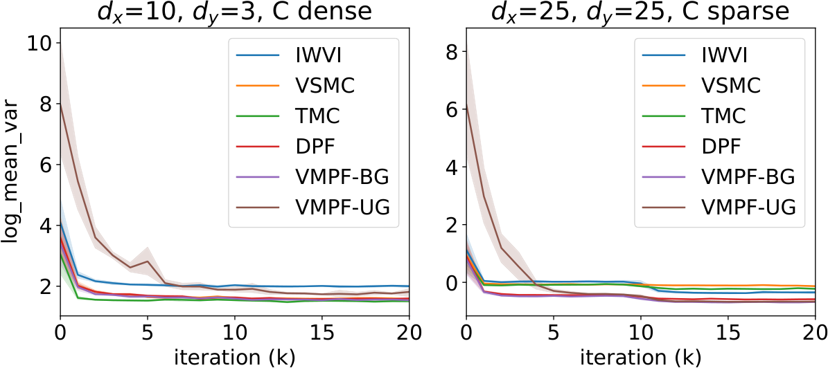

The slow convergence of VMPF-UG can be explained by gradient variance (Figure 2, left). Both VSMC and VMPF with biased gradients have low variance and converge quickly. In contrast, VMPF-UG has high gradient variance and slower convergence, especially in early iterations, but variance reduces substantially when close to convergence. This suggests a strategy of using the biased gradient estimator at the beginning of optimization and then switching to the unbiased estimator.
Although we did not observe it for , unbiased gradients can lead to tighter bounds upon convergence, especially for larger numbers of particles (Figure 2, right). For small , VMPF-BG and VMPF-UG are similar, but as increases, the gap between the methods increases, which indicates that biased gradients are more of a problem. We conjecture that the bias of gradients for VMPF-BG will not go to zero as is increased, but the magnitude of the true gradient shrinks as , which leads to difficulty in training (Le et al. 2018; Rainforth et al. 2018).
Stochastic Volatility
The stochastic volatility model (Chib et al. 2009) is widely used for financial data. It is where , , and . The model parameters are , where is a vector, and are diagonal matrices, and is either a diagonal or lower triangular matrix (with positive diagonal entries in both cases). We use VEM to learn . Following Naesseth et al. 2018, we use the proposal with parameters and diagonal.
| Method | |||||
|---|---|---|---|---|---|
| Diagonal | IWVI | 7216.09 (0.42) | 7219.77 (0.17) | 7220.60 (0.51) | 7221.51 (0.10) |
| VSMC | 7200.57 (0.11) | 7198.13 (0.30) | 7197.70 (0.09) | ||
| TMC | 7193.21 (0.08) | 7202.16 (0.07) | 7208.67 (0.11) | ||
| DPF | 7209.42 (0.99) | 7209.05 (1.13) | 7210.22 (0.24) | ||
| VMPF-BG | 7205.29 (0.17) | 7205.04 (0.16) | 7205.90 (0.35) | ||
| VMPF-UG | 7208.57 (0.27) | 7208.95 (0.28) | 7206.35 (0.27) | ||
| Triangular | IWVI | 8585.16 (1.00) | 8590.87 (0.27) | 8593.19 (0.64) | 8595.78 (0.82) |
| VSMC | 8573.04 (0.23) | 8572.58 (0.19) | 8572.01 (0.08) | ||
| TMC | 8554.89 (0.18) | 8570.56 (0.01) | 8582.32 (0.10) | ||
| DPF | 8572.74 (2.97) | 8574.32 (1.65) | 8574.32 (0.32) | ||
| VMPF-BG | 8576.57 (0.61) | 8578.53 (0.20) | 8581.21 (0.39) | ||
| VMPF-UG | 8556.64 (3.63) | 8543.40 (1.48) | 8538.15 (5.36) |
We model the exchange rates of 22 international currencies with respect to US dollars for 10 years (monthly from 4/2011 to 3/2021). The data can be downloaded from the US Federal Reserve System.‡‡ ‡ https://www.federalreserve.gov/releases/h10/current/ Table 1 reports the optimized lower bound for different algorithms for . VMPF-BG always gives a higher bound than VSMC, and the IWVI bound is always highest. TMC works well for , but is much worse for smaller . We also notice that DPF works slightly better than VSMC or VMPF on a simpler model with diagonal , but worse than VMPF with triangular . VMPF-UG is beneficial for diagonal with , but becomes increasingly harder to train with large and a larger model. The IWVI performance is surprising and contrary to similar experiments in (Naesseth et al. 2018), but appears to be another case where the family of proposal distributions can already approximate the posterior very well: we also find the ELBO with “vanilla” VI () is higher than SMC-based methods with in both cases.
Deep Markov Models
| Method | Nottingham | JSB | MuseData | Piano-midi.de | |
|---|---|---|---|---|---|
| 4 | IWVI | -3.86 (0.04) | -7.40 (0.01) | -8.19 (0.04) | -8.78 (0.01) |
| VSMC | -3.38 (0.03) | -7.16 (0.01) | -7.68 (0.02) | -8.39 (0.03) | |
| TMC | -3.65 (0.02) | -7.51 (0.01) | -8.41 (0.02) | -9.00 (0.01) | |
| DPF | -3.33 (0.02) | -7.14 (0.01) | -7.75 (0.01) | -8.45 (0.01) | |
| VMPF-BG | -3.29 (0.03) | -7.04 (0.01) | -7.67 (0.00) | -8.35 (0.01) | |
| 8 | IWVI | -3.82 (0.03) | -7.38 (0.01) | -8.16 (0.04) | -8.75 (0.01) |
| VSMC | -3.20 (0.02) | -6.96 (0.00) | -7.43 (0.01) | -8.20 (0.01) | |
| TMC | -3.40 (0.02) | -7.24 (0.01) | -8.03 (0.01) | -8.64 (0.01) | |
| DPF | -3.19 (0.00) | -6.95 (0.01) | -7.40 (0.01) | -8.31 (0.00) | |
| VMPF-BG | -3.09 (0.03) | -6.80 (0.01) | -7.39 (0.01) | -8.12 (0.01) | |
| 16 | IWVI | -3.84 (0.03) | -7.33 (0.02) | -8.16 (0.02) | -8.74 (0.02) |
| VSMC | -3.06 (0.02) | -6.81 (0.00) | -7.22 (0.02) | -8.03 (0.00) | |
| TMC | -3.23 (0.02) | -6.98 (0.02) | -7.72 (0.00) | -8.37 (0.01) | |
| DPF | -3.08 (0.02) | -6.78 (0.00) | -7.22 (0.01) | -8.18 (0.02) | |
| VMPF-BG | -2.96 (0.02) | -6.64 (0.01) | -7.14 (0.01) | -7.92 (0.01) |
We evaluate the bounds of all methods for deep Markov models (DMMs) on four polyphonic music datasets: Nottingham, JSB, MuseData and Piano-midi.de (Boulanger-Lewandowski et al. 2012). These are typically modeled with VRNNs, but the marginalization of ancestor variables prevents using VMPF for VRNNs (see Section 7 and the supplement). The DMM model is
where , , and , , are neural networks. To approximate the posterior, we define the proposal distribution
where , , and are neural networks. Details can be found in supplement. Table 2 shows the results of different methods. We see that in all cases VMPF-BG produces the best results. It is possible to train VMPF-UG in most settings here by initializing with VMPF-BG and/or using gradient clipping, but they lead to a slightly worse results than VMPF-BG.
7 Limitations
We are aware of several limitations or potential limitations. First, for VMPF-UG, implicit reparameterization gradients for mixture distributions require the ability to compute conditional CDFs of each component distribution (Graves 2016; Figurnov et al. 2018), which is straightforward for Gaussians or product distribution, but may be difficult in general. Current implementations support only product distributions (Dillon et al. 2017). At present, this limits the choice of proposals for VMPF-UG. There is no such limitation for VMPF-BG.
Second, although implicit reparameterization gives unbiased gradients for VMPF, we show that the variance remains high compared to VSMC and VMPF-BG, which restricts applying VMPF-UG in some cases, especially to complex models. Future work can focus on reducing the variance.
Third, unlike VSMC, VMPF only works for the the marginal objective , which restricts some applications, for example, to VRNNs (Chung et al. 2015). See the supplement for discussion.
Acknowledgements
We thank Javier Burroni, Tomas Geffner and the anonymous reviewers for comments that greatly improved the manuscript. This material is based upon work supported by the National Science Foundation under Grant Nos. 1749854, 1908577 and 2045900.
References
- Abadi et al. (2015) Martín Abadi, Ashish Agarwal, Paul Barham, Eugene Brevdo, Zhifeng Chen, Craig Citro, Greg S. Corrado, Andy Davis, Jeffrey Dean, Matthieu Devin, Sanjay Ghemawat, Ian Goodfellow, Andrew Harp, Geoffrey Irving, Michael Isard, Yangqing Jia, Rafal Jozefowicz, Lukasz Kaiser, Manjunath Kudlur, Josh Levenberg, Dandelion Mané, Rajat Monga, Sherry Moore, Derek Murray, Chris Olah, Mike Schuster, Jonathon Shlens, Benoit Steiner, Ilya Sutskever, Kunal Talwar, Paul Tucker, Vincent Vanhoucke, Vijay Vasudevan, Fernanda Viégas, Oriol Vinyals, Pete Warden, Martin Wattenberg, Martin Wicke, Yuan Yu, and Xiaoqiang Zheng. TensorFlow: Large-scale machine learning on heterogeneous systems, 2015. URL https://www.tensorflow.org/. Software available from tensorflow.org.
- Aitchison (2019) Laurence Aitchison. Tensor Monte Carlo: Particle methods for the GPU era. In Advances in Neural Information Processing Systems 32: Annual Conference on Neural Information Processing Systems 2019, NeurIPS 2019, December 8-14, 2019, Vancouver, BC, Canada, pages 7146–7155, 2019.
- Beal and Ghahramani (2003) Matthew J. Beal and Zoubin Ghahramani. The variational bayesian EM algorithm for incomplete data: with application to scoring graphical model structures. Bayesian statistics, 7(453-464):210, 2003.
- Blei et al. (2016) David M. Blei, Alp Kucukelbir, and Jon D. McAuliffe. Variational inference: A review for statisticians. Journal of the American Statistical Association, 112:859 – 877, 2016.
- Boulanger-Lewandowski et al. (2012) Nicolas Boulanger-Lewandowski, Yoshua Bengio, and Pascal Vincent. Modeling temporal dependencies in high-dimensional sequences: Application to polyphonic music generation and transcription. In Proceedings of the 29th International Conference on Machine Learning, ICML 2012, Edinburgh, Scotland, UK, June 26 - July 1, 2012. icml.cc / Omnipress, 2012.
- Branchini and Elvira (2021) Nicola Branchini and Víctor Elvira. Optimized auxiliary particle filters: adapting mixture proposals via convex optimization. In Proceedings of the 37th Conference in Uncertainty in Artificial Intelligence, UAI 2021, Online, July 27-30, 2021, 2021.
- Burda et al. (2016) Yuri Burda, Roger B. Grosse, and Ruslan Salakhutdinov. Importance weighted autoencoders. In 4th International Conference on Learning Representations, ICLR 2016, San Juan, Puerto Rico, May 2-4, 2016, Conference Track Proceedings, 2016.
- Campbell et al. (2021) Andrew Campbell, Yuyang Shi, Thomas Rainforth, and Arnaud Doucet. Online variational filtering and parameter learning. Advances in Neural Information Processing Systems, 34, 2021.
- Caterini et al. (2018) Anthony L. Caterini, Arnaud Doucet, and Dino Sejdinovic. Hamiltonian variational auto-encoder. In Advances in Neural Information Processing Systems 31: Annual Conference on Neural Information Processing Systems 2018, NeurIPS 2018, December 3-8, 2018, Montréal, Canada, pages 8178–8188, 2018.
- Chib et al. (2009) Siddhartha Chib, Yasuhiro Omori, and Manabu Asai. Multivariate stochastic volatility. In Handbook of financial time series, pages 365–400. Springer, 2009.
- Chung et al. (2015) Junyoung Chung, Kyle Kastner, Laurent Dinh, Kratarth Goel, Aaron C. Courville, and Yoshua Bengio. A recurrent latent variable model for sequential data. In Advances in Neural Information Processing Systems 28: Annual Conference on Neural Information Processing Systems 2015, December 7-12, 2015, Montreal, Quebec, Canada, pages 2980–2988, 2015.
- Corenflos et al. (2021) Adrien Corenflos, James Thornton, George Deligiannidis, and Arnaud Doucet. Differentiable particle filtering via entropy-regularized optimal transport. In Proceedings of the 38th International Conference on Machine Learning, ICML 2021, 18-24 July 2021, Virtual Event, volume 139 of Proceedings of Machine Learning Research, pages 2100–2111. PMLR, 2021.
- Dillon et al. (2017) Joshua V. Dillon, Ian Langmore, Dustin Tran, Eugene Brevdo, Srinivas Vasudevan, Dave Moore, Brian Patton, Alex Alemi, Matthew D. Hoffman, and Rif A. Saurous. Tensorflow distributions. arXiv preprint arXiv:1711.10604, 2017.
- Domke and Sheldon (2018) Justin Domke and Daniel R. Sheldon. Importance weighting and variational inference. In Advances in Neural Information Processing Systems 31: Annual Conference on Neural Information Processing Systems 2018, NeurIPS 2018, December 3-8, 2018, Montréal, Canada, pages 4475–4484, 2018.
- Domke and Sheldon (2019) Justin Domke and Daniel R. Sheldon. Divide and couple: Using Monte Carlo variational objectives for posterior approximation. In Advances in Neural Information Processing Systems 32: Annual Conference on Neural Information Processing Systems 2019, NeurIPS 2019, December 8-14, 2019, Vancouver, BC, Canada, pages 338–347, 2019.
- Douc and Moulines (2008) Randal Douc and Eric Moulines. Limit theorems for weighted samples with applications to sequential Monte Carlo methods. The Annals of Statistics, 36(5):2344 – 2376, 2008.
- Doucet and Johansen (2009) Arnaud Doucet and Adam M. Johansen. A tutorial on particle filtering and smoothing: Fifteen years later. Handbook of nonlinear filtering, 12(656-704):3, 2009.
- Figurnov et al. (2018) Mikhail Figurnov, Shakir Mohamed, and Andriy Mnih. Implicit reparameterization gradients. In Advances in Neural Information Processing Systems 31: Annual Conference on Neural Information Processing Systems 2018, NeurIPS 2018, December 3-8, 2018, Montréal, Canada, pages 439–450, 2018.
- Graves (2016) Alex Graves. Stochastic backpropagation through mixture density distributions. arXiv preprint arXiv:1607.05690, 2016.
- Han et al. (2016) Shaobo Han, Xuejun Liao, David B. Dunson, and Lawrence Carin. Variational Gaussian copula inference. In Proceedings of the 19th International Conference on Artificial Intelligence and Statistics, AISTATS 2016, Cadiz, Spain, May 9-11, 2016, volume 51, pages 829–838. JMLR.org, 2016.
- Harvey (1990) Andrew C. Harvey. Forecasting, Structural Time Series Models and the Kalman Filter. Cambridge University Press, 1990. doi: 10.1017/CBO9781107049994.
- Hirt et al. (2019) Marcel Hirt, Petros Dellaportas, and Alain Durmus. Copula-like variational inference. In Advances in Neural Information Processing Systems 32: Annual Conference on Neural Information Processing Systems 2019, NeurIPS 2019, December 8-14, 2019, Vancouver, BC, Canada, pages 2955–2967, 2019.
- Jang et al. (2017) Eric Jang, Shixiang Gu, and Ben Poole. Categorical reparameterization with gumbel-softmax. In 5th International Conference on Learning Representations, ICLR 2017, Toulon, France, April 24-26, 2017, Conference Track Proceedings, 2017.
- Jonschkowski et al. (2018) Rico Jonschkowski, Divyam Rastogi, and Oliver Brock. Differentiable particle filters: End-to-end learning with algorithmic priors. In Robotics: Science and Systems XIV, Carnegie Mellon University, Pittsburgh, Pennsylvania, USA, June 26-30, 2018, 2018.
- Jordan et al. (1999) Michael I. Jordan, Zoubin Ghahramani, Tommi S. Jaakkola, and Lawrence K. Saul. An introduction to variational methods for graphical models. Mach. Learn., 37(2):183–233, 1999.
- Karkus et al. (2018) Péter Karkus, David Hsu, and Wee Sun Lee. Particle filter networks with application to visual localization. In 2nd Annual Conference on Robot Learning, CoRL 2018, Zürich, Switzerland, 29-31 October 2018, Proceedings, volume 87 of Proceedings of Machine Learning Research, pages 169–178. PMLR, 2018.
- Kingma and Ba (2015) Diederik P. Kingma and Jimmy Ba. Adam: A method for stochastic optimization. In 3rd International Conference on Learning Representations, ICLR 2015, San Diego, CA, USA, May 7-9, 2015, Conference Track Proceedings, 2015.
- Kingma and Welling (2014) Diederik P. Kingma and Max Welling. Auto-encoding variational bayes. In 2nd International Conference on Learning Representations, ICLR 2014, Banff, AB, Canada, April 14-16, 2014, Conference Track Proceedings, 2014.
- Klaas et al. (2005) Mike Klaas, Nando de Freitas, and Arnaud Doucet. Toward practical N2 Monte Carlo: the marginal particle filter. In UAI ’05, Proceedings of the 21st Conference in Uncertainty in Artificial Intelligence, Edinburgh, Scotland, July 26-29, 2005, pages 308–315. AUAI Press, 2005.
- Krishnan et al. (2017) Rahul G. Krishnan, Uri Shalit, and David A. Sontag. Structured inference networks for nonlinear state space models. In Proceedings of the Thirty-First AAAI Conference on Artificial Intelligence, February 4-9, 2017, San Francisco, California, USA, pages 2101–2109. AAAI Press, 2017.
- Le et al. (2018) Tuan Anh Le, Maximilian Igl, Tom Rainforth, Tom Jin, and Frank Wood. Auto-encoding sequential Monte Carlo. In 6th International Conference on Learning Representations, ICLR 2018, Vancouver, BC, Canada, April 30 - May 3, 2018, Conference Track Proceedings, 2018.
- Lin et al. (2005) Ming T Lin, Junni L Zhang, Qiansheng Cheng, and Rong Chen. Independent particle filters. Journal of the American Statistical Association, 100(472):1412–1421, 2005.
- Liu and Liu (2001) Jun S Liu and Jun S Liu. Monte Carlo strategies in scientific computing, volume 10. Springer, 2001.
- Ma et al. (2020a) Xiao Ma, Péter Karkus, David Hsu, and Wee Sun Lee. Particle filter recurrent neural networks. In The Thirty-Fourth AAAI Conference on Artificial Intelligence, AAAI 2020, The Thirty-Second Innovative Applications of Artificial Intelligence Conference, IAAI 2020, The Tenth AAAI Symposium on Educational Advances in Artificial Intelligence, EAAI 2020, New York, NY, USA, February 7-12, 2020, pages 5101–5108. AAAI Press, 2020a.
- Ma et al. (2020b) Xiao Ma, Péter Karkus, David Hsu, Wee Sun Lee, and Nan Ye. Discriminative particle filter reinforcement learning for complex partial observations. In 8th International Conference on Learning Representations, ICLR 2020, Addis Ababa, Ethiopia, April 26-30, 2020. OpenReview.net, 2020b.
- Maddison et al. (2017a) Chris J. Maddison, Dieterich Lawson, George Tucker, Nicolas Heess, Mohammad Norouzi, Andriy Mnih, Arnaud Doucet, and Yee Whye Teh. Filtering variational objectives. In Advances in Neural Information Processing Systems 30: Annual Conference on Neural Information Processing Systems 2017, December 4-9, 2017, Long Beach, CA, USA, pages 6573–6583, 2017a.
- Maddison et al. (2017b) Chris J. Maddison, Andriy Mnih, and Yee Whye Teh. The concrete distribution: A continuous relaxation of discrete random variables. In 5th International Conference on Learning Representations, ICLR 2017, Toulon, France, April 24-26, 2017, Conference Track Proceedings, 2017b.
- Miller et al. (2017) Andrew C. Miller, Nicholas J. Foti, and Ryan P. Adams. Variational boosting: Iteratively refining posterior approximations. In International Conference on Machine Learning, pages 2420–2429. PMLR, 2017.
- Moretti et al. (2019) Antonio Khalil Moretti, Zizhao Wang, Luhuan Wu, Iddo Drori, and Itsik Pe’er. Particle smoothing variational objectives. arXiv preprint arXiv:1909.09734, 2019.
- Naesseth et al. (2015) Christian A. Naesseth, Fredrik Lindsten, and Thomas B. Schön. Nested sequential Monte Carlo methods. In Proceedings of the 32nd International Conference on Machine Learning, ICML 2015, Lille, France, 6-11 July 2015, volume 37 of JMLR Workshop and Conference Proceedings, pages 1292–1301. JMLR.org, 2015.
- Naesseth et al. (2018) Christian A. Naesseth, Scott W. Linderman, Rajesh Ranganath, and David M. Blei. Variational sequential Monte Carlo. In International Conference on Artificial Intelligence and Statistics, AISTATS 2018, 9-11 April 2018, Playa Blanca, Lanzarote, Canary Islands, Spain, volume 84 of Proceedings of Machine Learning Research, pages 968–977. PMLR, 2018.
- Naesseth et al. (2019) Christian A. Naesseth, Fredrik Lindsten, and Thomas B. Schön. Elements of sequential Monte Carlo. Found. Trends Mach. Learn., 12(3):307–392, 2019.
- Papamakarios et al. (2019) George Papamakarios, Eric Nalisnick, Danilo Jimenez Rezende, Shakir Mohamed, and Balaji Lakshminarayanan. Normalizing flows for probabilistic modeling and inference. arXiv preprint arXiv:1912.02762, 2019.
- Rainforth et al. (2018) Tom Rainforth, Adam Kosiorek, Tuan Anh Le, Chris Maddison, Maximilian Igl, Frank Wood, and Yee Whye Teh. Tighter variational bounds are not necessarily better. In International Conference on Machine Learning, pages 4277–4285. PMLR, 2018.
- Ranganath et al. (2016) Rajesh Ranganath, Dustin Tran, and David M. Blei. Hierarchical variational models. In Proceedings of the 33nd International Conference on Machine Learning, ICML 2016, New York City, NY, USA, June 19-24, 2016, volume 48, pages 324–333. JMLR.org, 2016.
- Rezende and Mohamed (2015) Danilo Jimenez Rezende and Shakir Mohamed. Variational inference with normalizing flows. In Proceedings of the 32nd International Conference on Machine Learning, ICML 2015, Lille, France, 6-11 July 2015, volume 37, pages 1530–1538. JMLR.org, 2015.
- Rezende et al. (2014) Danilo Jimenez Rezende, Shakir Mohamed, and Daan Wierstra. Stochastic backpropagation and approximate inference in deep generative models. In International conference on machine learning, pages 1278–1286. PMLR, 2014.
- Salimans et al. (2015) Tim Salimans, Diederik P. Kingma, and Max Welling. Markov chain Monte Carlo and variational inference: Bridging the gap. In Proceedings of the 32nd International Conference on Machine Learning, ICML 2015, Lille, France, 6-11 July 2015, volume 37, pages 1218–1226. JMLR.org, 2015.
- Stites et al. (2021) Sam Stites, Heiko Zimmermann, Hao Wu, Eli Sennesh, et al. Learning proposals for probabilistic programs with inference combinators. In Proceedings of the 37th Conference in Uncertainty in Artificial Intelligence, UAI 2021, Online, July 27-30, 2021, 2021.
- Sutton and Barto (2005) Richard S. Sutton and Andrew G. Barto. Reinforcement learning: An introduction. IEEE Transactions on Neural Networks, 16:285–286, 2005.
- Tran et al. (2015) Dustin Tran, David M. Blei, and Edoardo M. Airoldi. Copula variational inference. In Advances in Neural Information Processing Systems 28: Annual Conference on Neural Information Processing Systems 2015, December 7-12, 2015, Montreal, Quebec, Canada, pages 3564–3572, 2015.
- Tran et al. (2016) Dustin Tran, Rajesh Ranganath, and David M. Blei. Variational Gaussian process. In 4th International Conference on Learning Representations, ICLR 2016, San Juan, Puerto Rico, May 2-4, 2016, Conference Track Proceedings, 2016.
- van de Meent et al. (2018) Jan-Willem van de Meent, Brooks Paige, Hongseok Yang, and Frank Wood. An introduction to probabilistic programming. arXiv preprint arXiv:1809.10756, 2018.
- Zhu et al. (2020) Michael Zhu, Kevin Murphy, and Rico Jonschkowski. Towards differentiable resampling. arXiv preprint arXiv:2004.11938, 2020.
Supplementary Material:
Variational Marginal Particle Filters
Appendix A Proof of the Operations
A.1 Proof of Lemma 1
Proof.
We have that
For the variance, we have
For the lower bounds,
and because we have shown that and are valid estimator-coupling pair for . ∎
A.2 Proof of Lemma 2
Proof.
∎
A.3 Proof of Lemma 3
Proof.
For ExtendTarget,
For ChangeTarget, proceed as above with in place of . The steps are the same until the second to last line, which becomes
∎
Appendix B Derivation of SMC and MPF
B.1 Proof of Theorem 1
We first repeat relevant definitions from the algorithm and theorem statement. The weights are
The normalized weights are .
We wish to show that, for all ,
| (14) | ||||
| (15) | ||||
| (16) |
define an estimator-coupling pair for .
We can check that these match the SMC algorithm at step : that is, is sampling distribution, is the likelihood estimator, and is approximation to . So, after proving this, the conclusion of the theorem follows immediately.
We will show inductively that are obtained by applying appropriate operations on estimator-coupling pairs. In particular, the procedure is
where
and, for ,
The proof is a mechanical application of these operations.
For the base case, it is immediate that are an estimator-coupling pair for , and easy to verify that applying Lemma 2 yields that match Equations (14)–(16) and give an estimator-coupling pair for .
For the induction step (), we first apply Lemma 3 to obtain from using the ExtendTarget operation. We get
By Lemma 3, define an estimator-coupling pair for .
B.2 Proof of Theorem 2
We again repeat the relevant definitions. The weights used in VMPF are
The normalized weights are .
We wish to show that, for all ,
| (17) | ||||
| (18) | ||||
| (19) |
define an estimator-coupling pair for .
We can check that these match the MPF algorithm at step : that is, is sampling distribution, is the likelihood estimator, and is approximation to . So, after proving this, the conclusion of the theorem follows immediately.
We will show inductively that are obtained by applying appropriate operations on estimator-coupling pairs to. In particular, the procedure is
for all , where
and, for ,
The proof is again a mechanical application of these operations.
The base case is identical to the base case in the proof of Theorem 1, and yields that have the form in Equations (17)–(19) and define an estimator-coupling pair for .
For the induction step , we first apply Lemma 3 as in the proof of Theorem 1, except using the ChangeTarget operation instead of ExtendTarget, to get
which define an estimator-coupling pair for .
Next, we apply the Marginalize operation using Lemma 1. Marginalizing from gives
The conditional distribution is
The new estimator is the conditional expectation
The new coupling is
Appendix C Deriving MPF from IPF
We directly give the detail of IPF in Algorithm 3.
In line 4 of Algorithm 3, distinct permutations ( for any satisfying ) of should be generated. Proposition 1 of IPF (Lin et al. 2005) implies that for any test function ,
| (20) |
If , we have .
The idea of TMC is to draw many copies of each individual variable from independent proposal distributions, and then average over all (exponentially many) combinations of joint samples to get an unbiased estimator. We assume for each latent variable , we have samples , . So
| (21) |
will be an unbiased estimator for . Computing the summation in Equation (C) can be accelerated by summing over , , …, in order. If we define , then summing over gives
| (22) |
We can further define the boxed variable in Equation (C) by and continue the summation. This gives a filtering style framework as in Algorithm 4. In the end, will also be an unbiased estimator for .
C.1 Deriving TMC for SSM from IPF
C.2 Deriving MPF from TMC for SSM
The proposal distributions of IPF and TMC can be extended to condition on all past particles, i.e. (See 7.2 of Aitchison 2019 about non-factorized TMC), which includes the case of MPF. However, no formal theory supports any specific form of proposal distribution, such as the mixture distribution used by MPF. Additionally, full details of how to construct the non-factorised approximate posterior and ensure differentiability are not given. Finally, by using couplings to derive MPF and VMPF, we obtain the interpretation as auxiliary variable VI as described in the main text, which is not obvious from the unbiasedness result of Equation (20) alone.
This paper fills these gaps by deriving MPF from SMC directly and revealing the KL decomposition for VMPF. Now we verify that MPF is TMC with a specific mixture distribution. If we define and replace the proposal distributions for by , we will have for all and
| (23) |
Therefore, the weight computation of MPF is equivalent to Line 6 of Algorithm 4 if the specific mixture distribution is chosen. And we directly have the unbiased estimator
| (24) |
to be in the same form as MPF.
Appendix D Limitation on VRNN
A VRNN is a sequential latent variable model
where is constant and for . The variational posterior distribution is factorized as
We interpret a VRNN as a SSM that has both deterministic latent variables and stochastic latent variables . The full model is
To be clearer, we define to be the full latent variable, so the model becomes . VSMC can be used to learn the parameters of a VRNN. However, VMPF is not applicable to learning VRNN parameters. If we set the proposal distribution to be
the weighting function for VMPF for would become
We know that, in general, for all , the values will be different from each other. Due to the presence of Dirac function, the summation in the numerator as well as the denominator will only have one non-zero term, so VMPF collapses to VSMC. This failure can be understood in terms of marginalization: if we are able to access with MPF at , we can reconstruct the corresponding that generates , but should be marginalized.
Appendix E Experiment Details
We run all experiments on CPU. For models with multiple data, the batch size is 1. The experiment details can be found below.
E.1 Details of experiments on stochastic volatility models
Suppose the raw data of the exchange rate is , we get by
for . For both diagonal and triangular case, we restrict elements of to be in . For all algorithms, we train with the same learning rate scheduler (See Table 3), except for VMPF-UG for diagonal with , where we train with 0.3x of the listed learning rate. Further reducing the learning rate has little effect on the results. To stabilize the training of VMPF-UG, we use gradient clipping with threshold . With that, VMPF-UG for diagonal with are not stable in early iterations, and we only keep stable runs.
| Diagonal | Triangular | |||
|---|---|---|---|---|
| Phase | Learning Rate | Epochs | Learning Rate | Epochs |
| 1 | 0.01 | 50000 | 0.003 | 100000 |
| 2 | 0.001 | 50000 | 0.0003 | 100000 |
| 3 | 0.0001 | 50000 | 0.00003 | 100000 |
| 4 | 0.00001 | 50000 | 0.000003 | 100000 |
E.2 Details of experiments on deep Markov models
The four polyphonic music datasets are sequences of 88-dimensional binary vectors. Recall that the DMM is
where , , and , , are neural networks. The architectures are
where varies on different datasets. And we use the proposal distribution
where , , and are neural networks. The architectures are
For training, we use the default train, validation, and test set split. For all datasets, the learning rate, training epochs and hidden units can be found in Table 4. The comma separates different phases of training: we train with the larger learning rates for some epochs and reduce the learning rate for some additional epochs. We report the performance on test set with the best parameters during training determined by the validation set.
| Nottingham | JSB | MuseData | Piano-midi.de | |
| Learning Rate | 0.001,0.0001 | 0.001,0.0001 | 0.001,0.0001 | 0.001,0.0001 |
| Epochs | 500,100 | 1000,200 | 350,100 | 600,150 |
| Hidden Units | 128 | 64 | 128 | 128 |