Investigating the existence of gravitomagnetic monopole in M87*
Abstract
We examine the possibility for the existence of gravitomagnetic monopole () in M87* by using the results obtained from its first Event Horizon Telescope image. By numerically deducing the shadow sizes in Kerr-Taub-NUT (KTN) spacetime, we show that the shadow size increases with increasing for a fixed Kerr parameter in case of the KTN black hole, whereas for a KTN naked singularity it increases with increasing for a fixed if . In general, the asymmetry of shadow shape increases if the central dark object in M87 is a KTN/Kerr naked singularity instead of a KTN/Kerr black hole. We find that a non-zero gravitomagnetic monopole is still compatible with the current EHT observations, in which case the upper limit of cannot be greater than , i.e., for the prograde rotation (), and the lower limit of cannot be less than , i.e., for the retrograde rotation (). Moreover, if the circularity of the shadow can be measured on a precision of , the Kerr and KTN naked singularities can be falsified for M87*.
pacs
PACS-keydiscribing text of that key and PACS-keydiscribing text of that key1 Introduction
The Kerr spacetime is a stationary and axisymmetric vacuum solution of the Einstein field equation and it is described by only two parameters: mass and spin of the collapsed object. Although other axisymmetric vacuum solutions of the Einstein equation do exist, the most prominent solution among all of them is the Kerr geometry from the astrophysical point of view. The Event Horizon Telescope (EHT) has also recently mapped the central compact radio source of the elliptical galaxy M87 to a Kerr black hole with unprecedented angular resolution EHT1. Adopting the working hypothesis that M87 contains a Kerr black hole (see Sec. 7.4 of EHT5), i.e., spin parameter (see Sec. 1 of EHT5), the EHT collaboration has tried to show that the observed image is overall consistent with the expectations for the shadow of a Kerr black hole EHT1. However, the alternatives to the Kerr BH have not been ruled out, and it has been suggested EHT5 to consider whether the data is also consistent or not with alternative models for the central object of M87. For example, it is suggested that the BHs with NUT (Newman-Unti-Tamburino) charges nut could also be possible EHT5 instead of a Kerr BH. One primary purpose of the present paper is to show how the NUT charge affects the shadow size and shape and whether the existence of the NUT charge, aka gravitomagnetic monopole, can be ruled out or not in the central compact radio source of the elliptical galaxy M87. To show this, we use the observational parameter values of the first image of M87*, as released by the EHT collaboration. The second and most important purpose of this paper is to constrain the values of the Kerr parameter and the NUT parameter of M87*, if it contains the non-zero gravitomagnetic monopole.
It was argued that the Kerr superspinar (or Kerr naked singularity ckj; ckp) model for M87* is ruled out by the EHT2017 observations EHT5 since the shadows of Kerr naked singularities are substantially smaller and very asymmetric compared to those of Kerr BHs (see Sec. 8 of EHT1), although other alternatives to the Kerr BH are not ruled out. However, it has recently been shown in sc that the inferred circularity and size of the shadow of M87* do not exclude the possibility that this object might be a superspinar. Therefore, one cannot conclude whether M87* is a Kerr BH () or a Kerr superspinar (). Now, considering the ‘no body in nature is exactly nonrotating’ jh, if we want to test the existence of NUT charge in M87*, we should use the more general Kerr-Taub-NUT (KTN) spacetime instead of the Kerr spacetime. Referring to the recent work by sc, here we also do not exclude the possibility that M87* could be a KTN naked singularity (NS) wei. Thus, our ‘test’ includes both the KTN BHs and NSs.
The KTN spacetime is a stationary and axisymmetric vacuum 11 1 Here the vacuum is defined by the vanishing of the symmetric part of the Einstein tensor. Note that the antisymmetric part of the Einstein tensor of the KTN spacetime does not vanish along the axisymmetric pole (e.g., see the Einstein-Cartan theory beyond the classical general relativity; hehl. solution of the Einstein equation. As mentioned in EHT5, the KTN BH is within general relativity with an additional field, i.e., the Einstein-Hilbert action requires no modification rs2 to accommodate the NUT charge. Thus, the KTN solution is related to neither merely post Newtonian nor some modified theory rs; rs2. We note that Bonnor bon physically interpreted this NUT charge as ‘a linear source of pure angular momentum’ dow; rs, i.e., ‘a massless rotating rod’, which is a fundamental aspect of physics rs2. If the NUT charge vanishes, the KTN spacetime reduces to the Kerr spacetime. Similarly, if the Kerr parameter vanishes, the KTN spacetime reduces to the Taub-NUT spacetime which includes only two parameters : mass and NUT charge.
One intriguing feature that emerges here is, the Taub-NUT metric is not asymptotically flat mis in the sense that coordinates cannot be introduced for which . The Taub-NUT spacetime is not asymptotically flat as it contains a string of torsion that extends to the infinity, which is beyond the classical general relativity and sourced by the NUT charge hehl. On the other hand, the Taub-NUT space is asymptotically flat mis in the sense that the Riemann tensor vanishes () for as the Schwarzschild case. Note particularly that the curvature components, and therefore all invariants formed from the Riemann tensor, depend only on , and not on the other coordinates mis. Thus, the Taub-NUT metric is ‘an asymptotically zero curvature space which apparently does not admit asymptotically rectangular coordinates’ mis. Specifically, while the time-coordinate slices are intrinsically asymptotically flat bini; zs, the fact that as (see Eq. 1 below) implies that the spacetime is not asymptotically flat. The non-vanishing term leads to the anisotropy at due to the presence of , which is also the reason that the Taub-NUT metric may describe a homogeneous but not isotropic cosmological model mis. In reality, we consider our Universe as homogeneous and isotropic. Therefore, if any astrophysical object contains the gravitomagnetic monopole, in order to nullify its effect at infinity or in order to intact the character of our Universe as ‘homogeneous and isotropic’, other astrophysical object(s) of our Universe should also contain gravitomagnetic monopole, so that the total effects of gravitomagnetic monopoles can vanish. However, the Taub-NUT metric asymptotically coincides with the leading approximation for large of a KTN space pnas with electric mass and magnetic mass . The asymptotic structures of the Taub-NUT and KTN spacetimes have recently been analysed in details in Sec. IV C of bun and Sec. IV of vir respectively.
Note that the time coordinate in the Taub-NUT metric would be discontinuous at the axisymmetric pole, and the spacetime contains close timelike curves around the axisymmetric pole, which would raise the causality violation issue rs2; kag. Misner mis argued that the discontinuity in time could be eliminated by making the time coordinate periodic, but a periodic time would not describe reality. In this paper, we apply the Novikov self-consistency principle/conjecture (only self-consistent trips back in time would be permitted nov; fn) to avoid the causality violation for the phenomena occurring in M87*.
Interestingly, it was argued in pnas that a nonrotating black hole may be set in rotation through successive throwing of electric and magnetic monopoles into it, and after completion of this sequence of processes, a Kerr collapsed object could be formed. Performing the similar analysis on Taub-NUT space with only magnetic mass , one can set it in rotation and a KTN collapsed object could be formed (see Conclusions of pnas). It was also shown in pnas that these systems, as seen from large distances, are endowed with an angular momentum proportional to the product of the two kinds of charges/masses. Remarkably, this angular momentum associated with the charge-monopole/electric mass-magnetic mass system finally loses all traces of its exotic origin and is perceived from the outside as ‘common rotation’. Therefore, it is perhaps not totally inconceivable to think that, at least part of the rotation of some of the observed compact objects of our Universe, might come from their hiding ‘magnetic poles’ which have not yet been observed pnas.
It was once suggested in lnbl that the signatures of gravitomagnetic monopole aka NUT charge might be found in the spectra of supernovae, quasars, or active galactic nuclei (see also kag; liu; cc). However, the observational evidence of this aspect of fundamental physics was elusive. In a very recent paper, the first observational indication of the gravitomagnetic monopole has been reported cbgm, based on the X-ray observations of an astrophysical collapsed object: GRO J1655-40 and it has been shown there that the accreting collapsed object GRO J1655-40 could be better described with the more general KTN spacetime cbgm2, instead of the Kerr spacetime. Now, as the compact radio source at the core of the galaxy M87 forms the primary component of an active galactic nucleus (AGN), one could expect the existence of the gravitomagnetic monopole in M87* too. This also motivates us to hunting the existence of gravitomagnetic monopole in M87*.
One should note here that the shadow structures for the various spacetimes are recently investigated in several papers. For example, the shadow structures of a Kerr-like wormholes 1Amir, charged wormholes 3Amir, 5D electrically charged Bardeen black holes 4Jusufi, uncharged 2Ghosh and charged 6Kumar rotating regular black holes are thoroughly investigated. The shadow structures of a rotating black holes in 4D Einstein-Gauss-Bonnet gravity is also discussed in 5Kumar. The parameter estimation of different kinds of black holes have also been illustrated by constraints from the black hole shadow 7Kumar; afrin.
The scheme of the paper is as follows. In Sec. 2, we briefly describe the KTN spacetime. We outline the basic structure to study the BH shadow in Sec. 3 and apply it to the KTN spacetime. We constrain the value of gravitomagnetic monopole for M87* in Sec. 4, and finally we conclude in Sec. 5. Note that the geometrized units () are adpoted throughout the paper.
2 Kerr-Taub-NUT Spacetime
Before going into detail, we briefly describe the KTN spacetime below. The metric of the KTN spacetime is expressed as ml 22 2 Here, we use the same form of KTN metric that is considered in Eqs. (1-5) of ml and valid for . The case is the only possibility for the NUT solutions to have a finite total angular momentum, as shown in mr. In fact, the north and south poles play a symmetrical role for (see bun; vir). However, one may repeat the same analysis (which is presented in this manuscript) for the KTN metric including (see Eqs. 4.1–4.4 of vir). The discussions on the parameter could be found in kag; mr.
| (1) | |||||
with
| (2) |
where is the mass, is the Kerr parameter or spin parameter and is the NUT parameter or gravitomagnetic monopole of the collapsed object. The boundaries of the outer horizon is located at
| (3) |
Setting , one can obtain the location of singularity mcd at
| (4) |
in KTN spacetime. The above expression (Eq. 4) reveals that the singularity does not arise for , which indicates a singularity-free KTN BH, whereas for a KTN BH with , singularity arises at , covered by the horizon. The singularity can arise for , which could be a KTN BH or a KTN NS depending on the numerical values of and . Now, as the vanishes for , one can always obtain a KTN NS in this case, whereas a KTN BH with singularity (covered by the horizon) arises if the following condition is satisfied: .
One can see an interesting fact from Eq. (4) that the location of singularity (arisen only for ) can vary depending on the sign of and . In Kerr spacetime (), the singularity always lies at , whether represents the prograde rotation () or the retrograde rotation (). However, the presence of gravitomagnetic monopole can shift the location of singularity in the KTN spacetime, as seen from Eq. (4). For instance, four possibilities can be arisen, which is discussed below dividing into four quadrants.
Quadrant I ( and ): The location of singularity can vary from to for to , or, for to .
Quadrant II ( and ): The location of singularity can vary from to for to , or, for to .
Quadrant III ( and ): The location of singularity can vary from to for to , or, for to .
Quadrant IV ( and ): The location of singularity can vary from to for to , or, for to .
We should note here that all the above mentioned four quadrants also include the singularity-free KTN BH regions which arises due to .
3 Shadow of a collapsed object
There are three types of photon trajectories fired from the large radii around a collapsed object: capture, scatter to infinity and critical curve. The latter or unstable curve separates the first and second types. If the 3-momentum of a light ray is nearly tangential to the circular photon orbit, the orbit is unstable and this ray orbits around the collapsed object several times. This light ray is either scattered to infinity or captured by the central object due to a small perturbation. As they orbit around the collapsed object several times, they create a brighter region around a central dark region in the sky plane of distant observer. This can be projected as a 2D image and the dark region of it is called as the shadow of that collapsed object.
In order to study shadow of a collapsed object, one needs to solve the geodesic equations. Here, we solve the geodesic equations numerically for the KTN metric using the ray tracing code. This is an initial value problem and to calculate the boundary of shadow we use the simulation with the assumption of stationarity 33 3 It is important to mention here that the assumption of stationarity removes the possibility of temporal signatures in the simulation. Thus, in practice a trajectory of the light exactly passing the pole where the discontinuity in (as discussed in Sec. 1) arises, does not exist in the simulation., similarly as that done in myshadow1; myshadow2. A class of Runge-Kutta-Nystrom method is used, which is explained in Lund:2009zzb. We use adaptive step sizes in our calculations with error control. We start from the observer’s sky plane, the location of which is expressed in the Cartesian coordinates and the collapsed object is located at . The observer’s plane is located at a distance away from the collapsed object, and at an inclination angle (see the geometry of the system in Figure 1 of js2). Photon’s initial 4-momentum, , is perpendicular to the observer plane. The image plane contains a grid and the photons are fired from every point of the grid. The ray is traced-back from each pixel of image with the initial condition to the collapsed object.
Now, we can write the initial condition coba for our simulation as:
| (5) |
The initial condition for the photon 4-momentum is :
| (6) |
where is obtained from the condition with the metric tensor of flat space time.
Boundary of the shadow of a collapsed object is a closed curve in the observer’s plane and it separates captured photon from scattered ones. To have image of the shadow boundary, we first define the center of a shadow in analogy with the center of mass calculation,
| (7) |
where represents inside of the shadow and represents the outside of it.
We consider axis as the symmetry axis of shadow boundary. We start from the shorter segment in axis with , and define as the distance between each point of the boundary and the center.
Figure 1 shows the examples for the cases with , , , and , i.e., the Schwarzschild metric, Kerr metric, KTN BH, and KTN NS for a particular inclination angle, say, . For different settings of , as it is shown in this Figure, the shadow sizes differ significantly, but the shapes are nearly circular and only have slight differences. For instance, the shadow is circular for the Schwarzschild BH, whereas it slightly deviates from the circularity even if increases to a large value for the Kerr BH, as shown in EHT5. For a fixed , the shadow size increases with increasing , but it is almost circular for the KTN BH cases and it becomes asymmetric for the KTN NS cases. However, the deviation from circularity is on the order of percentage level or less. For example, it is only if .
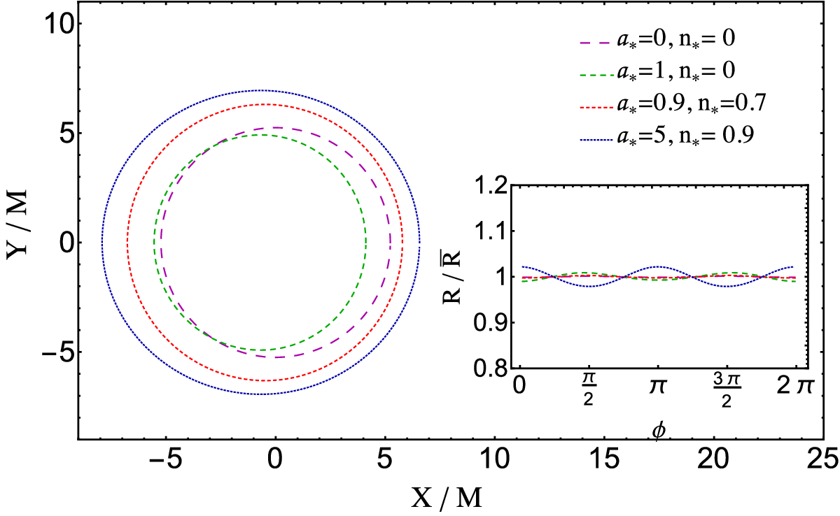
Now, it is asserted by the EHT collaboration that the recently released image of the shadow of M87* is not exactly circular EHT1, i.e., it deviates from circularity. Therefore, one needs to define the average radius of the shadow which can be expressed as (see Eq. 4 of sc)
| (8) |
Following sc; EHT1 one may also define a parameter to describe the asymmetry of shadow by using the difference between the RMS distance and the average radius of the shadow :
| (9) |
Here, the asymmetry parameter quantifies the deviation from circularity of the shadow. This parameter can also be used to compare the theoretically predicted shadow size of a collapsed object with the observational one. Below we first briefly discuss the theoretically predicted values of shadow size and circularity for the KTN spacetime in Secs. 3.1 and 3.2, respectively. Later, using the theoretical values and the recently reported observational parameter values of EHT, we constrain the gravitomagnetic monopole/NUT charge for M87* in Sec. 4.
3.1 Dependence of the shadow size on , , and


Figure 2 is drawn for four different inclination angles to show the variation of shadow sizes with the Kerr and NUT parameters (in unit of the mass scale ), as obtained theoretically. Our results are consistent with the shadow sizes obtained in tak (see also js1; js2) for Kerr BHs. In case of the Kerr BH, the shadow size first decreases with increasing the value of , until . It faces a sudden decrement in its value for further increment in , i.e., where . The latter one stands for an extreme case of Kerr NS. Interestingly, the shadow size increases with increasing the value of for Kerr NS, i.e., to a higher value, which is true for all inclination angles (see Figure 2). The physical reason behind this may be understood by considering the example of the behavior of corotating equatorial circular photon orbit (CPO). In the case of the Kerr BH, the radius of CPO, , comes closer and closer to the event horizon with increasing the value of (i.e., for ), whereas is always located (formally) at the ring singularity () chastu in the case of the Kerr NS. This means that the can exist very close to the ring singularity for all values of , in principle. One intriguing behavior of the ring singularity that emerges is, its radius increases with increasing (see Figure 2 of ckj), and hence, the CPO also becomes bigger and bigger in principle. This can be realized from the Kerr-Schild coordinates which reduce to ch :
| (10) |
Thus, the ring singularity ( in the Boyer-Lindquist coordinates) can be expressed as (see Figure 25 of ch)
| (11) |
Eq. (10) shows that the radius (in the Kerr-Schild coordinates) of () for is . Now, for a nearly extremal naked singularity (NENS), say, , the radius of CPO is : . It is needless to say here that the radius of CPO increases with the further increment of for the Kerr NS. The above discussion gives a rough idea that why the shadow size first decreases for the ‘transition’ from the extremal BH to a NENS and then increases again.
Note here that the shadow size varies from to for the Kerr BH with spin () varying from to for the inclination angles, i.e., (see Figure 2 of tak). One can see exactly the opposite scene for the Taub-NUT BH, i.e., KTN BH with . In this case, the shadow size increases with increasing the value of , but it does not change with the value of , as the Taub-NUT spacetime is spherically symmetric mis; lnbl. The different nature of these two parameters is reflected in the shadow size of KTN BH. In general, the shadow size increases with increasing for a fixed value of in case of the KTN BH. In contrast, it can increase or decrease with increasing for a fixed value of in case of the KTN NS. This statement is true for any inclination no matter whether it is a KTN BH or a KTN NS, which is also clear from Panels (a)–(d) of Figure 2 as well as 44 4 Figure 3 is, in fact, the extensive version of Panel (b) of Figure 2 with all of the four quadrants, as this particular plot is also necessary to constrain and for M87* using Figure 6. As the feature of the shadows for all inclination angles are almost similar to Figure 3, we do not repeat it by plotting Panels (a), (c) and (d) of Figure 2 for all of the four quadrants.Figure 3.


The appearance of the special feature (decreasing the shadow size for the transition from the extremal BH to the NENS) in the violet colored region of Figure 3 is not unusual in case of a NENS as discussed at the end of the first paragraph of this section. However, this explanation is true only for the KTN spacetime with the value of , if one moves along the axis with a constant value of . For a general large parameter space, the violet colored regions adjacent to the green dashed lines, shifts towards the right (left) side of the plot in Quadrant IV (Quadrant II), and the subsequent rainbow color appears at adjacent to the green dashed line. This means that the shadow sizes of KTN NENSs can be much bigger () than zero in such a case. Not only this, it is also shown that if (location of the singularity, see Eq. 4) is bigger than the inclination angle (), i.e., , one can see an extremely smaller shadow, whereas the shadow will be much bigger for . The above statement is true in either way, i.e., depending on a slight change in from (i.e., ), one can see a large difference in the shadow size of a same KTN object. For example, if we consider a KTN NS with , i.e., , one can see the shadow size of the object as with for , whereas the shadow size becomes with for . The reason behind these interesting discontinuity effects is due to an important relation between and , which is vividly discussed in Appendix A.
3.2 Dependence of the shadow circularity on , , and
Earlier it was shown in abdu that the NUT parameter not only increases the size of the KTN BH shadow (with the same and ), but it also circularize the BH shadow ellipse55 5 Although it is asserted as the ‘ellipse’ in abdu, it should be actually regarded as the ‘distorted form of a circle’. The increment of BH’s angular momentum distorts the ‘circular’ form of shadow but it does not take the shape of shadow to an exact form of ‘ellipse’. See Figure 4 and the end of Sec. 3 of abdu for details. However, this simpler description helps one to realize here the ‘opposite behavior’ of the Kerr parameter and the NUT parameter in a better way. Therefore, we continue our discussion in this paper following abdu, i.e., we use the word ‘ellipse’ or ‘elliptical’, instead of the ‘distorted form of a circle’, keeping in mind that the word ‘ellipse’ does not mean here an exact form of ellipse or elliptical shape in mathematics. abdu. The first property can be seen from Figure 2, and the second one from Figure 4. The left side of green dashed line of Figure 4 represents the KTN NS region whereas its right side represents the KTN BH region. Panel (a) of Figure 4 shows that the shadow of KTN BH becomes circular with increasing the value of for . The Kerr parameter tries to make it further elliptical. Comparing panels (a) and (b) of Figure 4, one can see this interesting difference of the Kerr and NUT parameters for the KTN BH. The same figures also show that the shadows are in general elliptical for in the case of KTN NSs.


Now, due to the small increment in from (i.e., equivalent to the Kerr spacetime) to , Panel (a) of Figure 5 spans the inclination and spin parameter region. The colored region represents the deviation from circularity which is less than or as defined in Eq. (9). As we have already mentioned that our probe includes both the BH as well as NS region, the left side of the green dashed line represents the KTN BHs whereas right side of the same represents the KTN NSs. The green dashed line stands for the extremal KTN BH. The maximum allowed value of inclination for is less than . If we further increase (decrease) the value of , the shadow size will be larger (smaller) and the hatched region in KTN NS moves to the smaller (larger) value of the spin parameter. This can be seen by comparing Panels (a) and (b) of Figure 5.
Figure 6 is drawn with the combinations of and for a fixed inclination angle, . The presence of thin Yellow-Cyan (YC) region along the green dashed line of this figure indicates that a high deviation of circularity with can be possible in Quadrants II and IV. For the general large parameter space, the thin YC regions, adjacent to the green dashed lines of Quadrants II & IV, are broadened for increasing the value of .
4 Constraining the gravitomagnetic monopole in M87*
It was suggested in EHT5 that the possibility for M87* being a Kerr NS is ruled out by arguing that the shadows of Kerr NSs () are substantially smaller and very asymmetric compared to those of Kerr BHs. Referring to the discussion of Sec. 3.1, we can say that the argument given in EHT5 is shaky. This can also be seen from Figure 2 (b) that one can obtain a short range of for which the shadow size is comparable to the Kerr BHs. This is recently shown by sc as well. However, there is a basic difference between that work sc and our present work. They considered one extra parameter, , which governs the scale at which quantum gravity effects become relevant. Therefore, they obtained two different ranges of for which M87* could be a superspinar. These are: for and for . In our case, we do not consider that extra parameter for the KTN NS. This means, we consider up to , i.e, is considered for our work. That is why, we obtain (see Figure 2(b)) the allowed range for M87* as for . It is useful to mention here that we restrict our probe for the KTN NS up to in this paper. We do not consider the KTN NS with a boundary at a positive value of unlike those presented in sc. This also means that the quantum gravity effects are considered not to be relevant gh; ckp for for this work.
To quantify our results we first consider the recently reported observational constraints by the EHT collaboration EHT6 on the shadow size of the BH in M87 as EHT1; sc
| (12) |
for (mass of M87*) and (average diameter of the crescent) arcsec EHT6. Although the distance of M87* is Mpc, we consider Mpc in the above equation for the simplification of our calculation following sc. Considering the KTN metric (Eq. 1) and observed parameter values, one can now constrain the value of NUT charge in M87* for Eq. (12). It is needless to say here that we use the KTN metric instead of the Kerr metric which was used in EHT1; sc. We also follow the limit of : EHT1, as reported by the EHT collaboration.
Here, Figure 4 shows how the allowed region of the shadow size of M87* varies with for a fixed value of , irrespective of the inclination angle. Especially the hatched region of this figure shows the allowed size of shadow according to Eq. (12). This implies that although the high value of inclination angle is satisfied for the KTN BH, it is excluded for the KTN NS by the circularity condition of the shadow of M87*. If we increase the value of , the size of the shadow will be smaller and the hatched region moves from the right to left, i.e., BH to NS region. It also shows that allowed values of the inclination angle decreases with the increasing value of . Interestingly, the shadow size of M87* does not only exclude the KTN BH for , but also excludes the high value of inclination angle. This is shown by the hatched region of Panel (c) of Figure 5 that the following range of with is only compatible with the circularity condition of M87* for this particular case.
Now, as mentioned, Figure 6 is drawn for to show the combinations of and which could be relevant for M87*. This assumption is made based on the estimated angle between the approaching jet (parallel/anti-parallel to spin direction) and line of sight by jet, that leads to the value as . The jet direction is controlled by the BH spin. If the BH spin axis is aligned with the jet, then the asymmetry of the shadow implies that the black hole spin is pointing away from Earth, i.e., the rotation of the BH is clockwise () as viewed from Earth (see Fig. 5 of EHT5). In Figure 6, we plot all of the four quadrants, as discussed at the end of Sec. 2 (we do not repeat here it again). A close observation of our results reveals that the features of hatched region in Quadrants I and III are same, whereas the features of Quadrants II and IV are same. Thus, we describe below these two different features separately.
h

4.1 Quadrants I and III
One can see from the plots of Quadrants I and III that M87* is not allowed as a KTN BH for the high value of , i.e., . For instance, if M87* is a KTN BH with , the value of has to be less than . If M87* is a KTN BH, the allowed ranges are and . To be a KTN NS, the allowed ranges are and . The upper limit of the NUT charge which could be contained in M87*, is . In that case, the value of the spin parameter will be . Quadrants I and III of Figure 6 and the above mentioned two separate ranges imply that there is a degeneracy in the value of , i.e. for , M87* could be a KTN BH or a KTN NS. This degeneracy could be broken by analyzing the deviation of circularity of the shadow of M87* more accurately. To be a KTN BH with , the shadow should be almost circular (i.e., ) whereas, it can significantly deviate from circularity if M87* is a KTN NS with , as seen from Quadrants I and III of Figure 6.
4.2 Quadrants II and IV
One can see from the plots of Quadrants II and IV of Figure 6 that M87* is allowed as a KTN BH for the low value () as well as the high value () of , unlike Quadrants I and III. In fact, the value of of M87* as a KTN BH or NS can be greater than even (i..e, ), which is not shown in the plot. To be a KTN NS of much lower value of (i.e., ), the allowed ranges for starts from . We plot Figures 3 and 6 for a limited parameter space. For a general large parameter space, much higher values of and/or are possible for M87* as a KTN BH or a KTN NS in Quadrants II and IV, if we compare it to the other two quadrants (I and III). For instance, the black hatched region of NS, which spans with (i.e., ) for , shifts towards right (left) of the plot in Quadrant IV (Quadrant II) with the higher values of for increasing the value of . As an example, the black hatched region of NS extends in the following range of for . However, the width of black hatched region of NS remains almost constant () for a fixed value of in the following range: . Not only this, the value of also remains almost constant (i.e., ) for the above-mentioned black hatched region of NS.
As it is seen from the discussion of Sec. 3.2 that, for the general large parameter space, the thin YC regions, adjacent to the green dashed lines, are broadened for increasing the value of , and the black hatched region of NS can be overlapped with this region. Note that the value of in the black hatched regions of NS is not necessarily always be within as shown in the limited parameter space of Figure 6, it can also be equal to or greater than (i.e., ) depending on the values of & in the general large parameter space, specifically close to the green dashed lines. For example, if M87* is a KTN NS of Quadrant IV with and , the shadow size would be with .
5 Conclusion and discussion
The KTN metric is the mathematical solution of the Einstein field equation, and the EHT observations EHT5 have not ruled out the possibility of M87* containing the gravitomagnetic monopole/NUT charge, yet. In this work, we have investigated the possibility for the existence of gravitomagnetic monopole in M87*, by studying how the shadow size and shape depends on the KTN metric parameters and using the first observational image of its shadow as constraints. We have found that the observational constraints on the size and circularity of the M87* shadow do not exclude the possibility that this compact object can be a naked singularity and contain the gravitomagnetic monopole. It is, therefore, important to have accurate measurements of both the shadow size and asymmetry, which can be used to put strong constraints on and , and break the degeneracies between the different metrics as well as between the BHs and NSs. If M87* is really a KTN NS, the accurate measurements of both the shadow size and asymmetry can help to break the degeneracies between the different quadrants.
Secondly, our finding reveals that the observational image is not only compatible with the KTN
metric of the limited ranges of and as shown in
Figure 6, but it is also compatible with the general large parameter space as discussed in Sec. 4.
Furthermore, we have also shown that if M87* in fact contains the gravitomagnetic monopole
the upper limit of cannot be greater than , i.e., in case of the prograde rotation (), whereas the lower limit
of cannot be less than , i.e., in case of the retrograde rotation (). If the deviation from the circularity of the shadow is found to be less than by the future EHT-like observations (such as, ngEHT ng), the Kerr and KTN NSs are falsifiable. In spite of that, M87* could still be described as a KTN BH with the upper limit of as in case of the prograde rotation (), and the lower limit of as in case of the retrograde rotation (). Note that our conclusion can be true, if M87* as a AGN (see lnbl) contains the NUT charge.
Acknowledgments
This work is partly supported by the National Key Program for Science and Technology Research and Development (Grant No. 2016YFA0400703, 2016YFA0400704), the National Natural Science Foundation of China under grant No. 11873056, 11690024, 11673001, 11750110410, 11721303, and the Strategic Priority Program of the Chinese Academy of Sciences (Grant No. XDB 23040100). M. G.-N. and C. C. acknowledge support from the China Postdoctoral Science Foundation, Grant No. 2017LH021 and 2018M630023 respectively.
Appendix A Relation between and in the Kerr-Taub-NUT spacetime
General case: Eq. (4) shows that although the singularity is always located at the equatorial plane: in the Kerr spacetime, this is not true for the KTN spacetime. Therefore, one can write Eq. (4) as
| (13) |
Now, substituting this (Eq. 13) into the basic NS condition:
| (14) |
we obtain
| (15) | |||||
| (16) | |||||
| (17) |
The corresponding value of can be obtained from Eq. (13) as :
| (18) | |||||
| (19) |
Below we discuss only for Quadrant IV, as the discussion on Quadrant II is similar to this one. For a fixed value of in Figure 3, the shadow size starts to decrease rapidly if one crosses (not for crossing ). This is valid for those values of which satisfy: . In contrast, the shadow size suddenly becomes very small due to crossing (which is similar to the Kerr case) for those values of which satisfy: . This term () does not show any interesting effect for the later case, as its value falls in the BH region, i.e., , but it plays an important role if its value falls in the NS region, i.e., . We have already calculated that this term comes outside of the BH region from this particular point ()66 6 also satisfies the condition of the extremal BH, i.e., the horizon is located at
| (20) |
This means that one can see its effect beyond this particular point and in that case this particular term () plays an important role for the size of the shadow. In this special case, the shadow of KTN NENSs can be much bigger (comparing to the Kerr NENSs) for the following range of but it starts to decrease rapidly for crossing the point for a fixed and eventually becomes very small. After that the shadow size increases again. Due to the same reason, the shadow size does not appear to be smaller for the transition from the extremal BH to NENS for . Thus, if one moves from (extremal BH) towards right along the axis with a fixed , one cannot see any abnormality in the shadow size for the transition from the extremal BH to NENS. The violet colored region adjacent to the green dashed line of Figure 3 is, therefore, shifted towards the right side of the plot. This special transition (shadow starts to decrease rapidly) occurs at for a fixed .
Application to the recent EHT result for M87*
The above mentioned scenario can be discussed considering an example of the recent EHT result for M87*. In this case, the transition starts at the point (see Eq. 20)
for in Quadrant IV. Therefore, the violet colored region of Figure 3 will be shifted towards the right side of the plot for (specifically from this point: ). For this case, if we move from the green dashed line of Figure 3 towards right (i.e., ) along a fixed , one cannot see any abnormality in the shadow size for the transition from the extremal BH to NENS. However, the violet colored region still remains adjacent to the green line for . The special transition (shadow starts to be smaller rapidly) occurs at for a fixed . The whole picture is also clear from the values given in Table 1.
| Shadow size | |||||
| 1.00 | 0.002 | 10.60 | |||
| -1 | 1.41 | 1.05 | 1.40 | 0.012 | 8.73 |
| 1.50 | 0.050 | 0.567 | |||
| 2.00 | 0.005 | 10.95 | |||
| -2 | 2.24 | 2.09 | 2.20 | 0.015 | 9.38 |
| 2.30 | 0 | 0.703 | |||
| -3.27 | 3.42 | 3.42 | 3.40 | 0.024 | 10.18 |
| 3.44 () | 0 | 0.003 | |||
| 4.12 | 0.038 | 10.38 | |||
| 4.16 () | 0.096 | 11.23 | |||
| -4 | 4.12 | 4.18 | 4.18 () | 0.025 | 7.43 |
| 4.20 () | 0 | 0.003 | |||
| -6 | 6.08 | 6.27 | 6.25 () | 0.108 | 13.45 |
| 6.29 () | 0 | 0.003 | |||
| -8 | 8.06 | 8.36 | 8.34 () | 0.117 | 15.57 |
| 8.38 () | 0 | 0.003 |
Interestingly, a deeper study of the values given in Table 1 reveals that, if is greater than the inclination angle (), i.e., , one can see an extremely smaller shadow, whereas the shadow will be much bigger for . The above statement is true in either way, i.e., depending on a slight change in the inclination angle from the location of singularity, one can see a huge difference in the shadow size of a same KTN object. This does not arise in case of the Kerr spacetime (), as
| (22) |
is a constant for any value of . Therefore, the rapid decreasing in the shadow sizes always occurs at , during the transition from the extremal Kerr BH to the Kerr NENS for any inclination angle .
References
- (1) The Event Horizon Telescope Collaboration, Astrophys. J. 875, L1 (2019).
- (2) The Event Horizon Telescope Collaboration, Astrophys. J. 875, L5 (2019).
- (3) E. Newman, L. Tamburino, T. Unti, J. Math. Phys. 4, 915 (1963).
- (4) C. Chakraborty, P. Kocherlakota, P. S. Joshi, Phys. Rev. D 95, 044006 (2017).
- (5) C. Chakraborty, P. Kocherlakota, M. Patil, S. Bhattacharyya, P. S. Joshi, A. Królak, Phys. Rev. D 95, 084024 (2017).
- (6) C. Bambi, K. Freese, S. Vagnozzi and L. Visinelli, Phys. Rev. D 100, 044057 (2019).
- (7) J. B. Hartle, Gravity:An introduction to Einstein’s General relativity, Pearson (2009).
- (8) S-W. Wei, Y-X. Liu, C-E Fu, K. Yang, JCAP 10 (2012) 053.
- (9) S. Ramaswamy, A. Sen, Phys. Rev. Lett. 57, 1088 (1986).
- (10) S. Ramaswamy, A. Sen, J. Math. Phys. (N.Y.) 22, 2612 (1981).
- (11) W. B. Bonnor, Proc. Camb. Phil. Soc. 66, 145 (1969).
- (12) J. S. Dowker, Gen. Rel. Grav. 5, 603 (1974).
- (13) C. W. Misner, J. Math. Phys. 4, 924 (1963).
- (14) F. W. Hehl, P. v. d. Heyde, G. D. Kerlick, Rev. Mod. Phys. 48, 393 (1976).
- (15) D. Bini et al., Class. Quantum Grav. 20, 457 (2003).
- (16) R. L. Zimmerman, B. Y. Shahir, Gen. Rel. Grav. 21, 821 (1989).
- (17) C. Bunster, M. Henneaux, PNAS 104, 12243 (2007).
- (18) C. Bunster et al., Phys. Rev. D 73, 105014 (2006).
- (19) A. Virmani, Phys. Rev. D 84, 064034 (2011).
- (20) V. Kagramanova et. al, Phys. Rev. D 81, 124044 (2010).
- (21) I. D. Novikov, Evolution of the Universe, Cambridge University Press, New York (1983)
- (22) J. Friedman et al., Phys. Rev. D 42, 1915 (1990)
- (23) D. Lynden-Bell, M. Nouri-Zonoz, Rev. Mod. Phys. 70, 427 (1998).
- (24) C. Liu, S. Chen, C. Ding, J. Jing, Phys. Lett. B 701, 285 (2011).
- (25) C. Chakraborty, Eur. Phys. J. C 75, 572 (2015).
- (26) C. Chakraborty, S. Bhattacharyya, Phys. Rev. D 98, 043021 (2018).
- (27) C. Chakraborty, S. Bhattacharyya, JCAP 05 (2019) 034.
- (28) M. Amir, K. Jusufi, A. Banerjee, S. Hansraj, Class. Quant. Grav. 36, 215007 (2019).
- (29) M. Amir, A. Banerjee and S. D. Maharaj, Annals Phys. 400, 198 (2019).
- (30) K. Jusufi, M. Amir, M. S. Ali, S. D. Maharaj, Phys. Rev. D 102, 064020 (2020).
- (31) S. G. Ghosh, M. Amir, S. D. Maharaj, Nucl. Phys. B 957, 115088 (2020).
- (32) R. Kumar, S. G. Ghosh, A. Wang, Phys. Rev. D 100, 124024 (2019).
- (33) R. Kumar, S. G. Ghosh, JCAP 07, 053 (2020).
- (34) R. Kumar, S. G. Ghosh, Astrophys. J. 892, 78 (2020).
- (35) M. Afrin, R. Kumar and S. G. Ghosh, Mon. Not. Roy. Astron. Soc. 504, 5927 (2021).
- (36) J. G. Miller, J. Math. Phys. 14, 486 (1973).
- (37) V. S. Manko, E. Ruiz, Class. Quantum Grav. 22, 3555 (2005).
- (38) S. Mukherjee, S. Chakraborty, N. Dadhich, Eur. Phys. J. C 79, 161 (2019).
- (39) M. Ghasemi-Nodehi, Z. Li and C. Bambi, Eur. Phys. J. C 75, 315 (2015).
- (40) M. Ghasemi-Nodehi, C. Bambi, Eur. Phys. J. C 76, 290 (2016).
- (41) E. Lund, L. Bugge, I. Gavrilenko and A. Strandlie, JINST 4, P04001 (2009).
- (42) T. Johannsen, D. Psaltis, Astrophys. J. 718, 446 (2010).
- (43) C. Bambi, Astrophys. J. 761, 174 (2012).
- (44) R. Takahashi, Astrophys. J. 611, 996 (2004).
- (45) T. Johannsen, D. Psaltis, Astrophys. J. 716, 187 (2010).
- (46) D. Charbulak, Z. Stuchlik, Eur. Phys. J. C 78, 879 (2018).
- (47) S. Chandrashekar, The Mathematical Theory of Black Holes, Clarendon Press, Oxford (1983).
- (48) A. Abdujabbarov et al., Astrophys. Space. Sci. 344, 429 (2013).
- (49) E. G. Gimon, P. Horava, Phys. Lett. B 672, 299 (2009).
- (50) The Event Horizon Telescope Collaboration, Astrophys. J. 875, L6 (2019).
- (51) R. Craig Walker, P. E. Hardee, F. B. Davies, C. Ly and W. Junor, Astrophys. J. 855, 128 (2018).
- (52) The Next Generation Event Horizon Telescope (ngEHT): https://pweb.cfa.harvard.edu/news/announcement-next-generation-event-horizon-telescope-design-program