Matching Markets

Andrew Yang Affiliation: Department of Linguistics Affiliation: Stanford University Email: ycm@stanford.edu Bruce Changlong Xu Affiliation: Department of Computer Science Affiliation: Stanford University Email: bcxu1506@stanford.edu Ivan Villa-Renteria Affiliation: Department of Computer Science Affiliation: Stanford University Email: ivillar@stanford.edu

Abstract

Matching markets are of particular interest in computer science and economics literature as they are often used to model real-world phenomena where we aim to equitably distribute a limited amount of resources to multiple agents and determine these distributions efficiently. Although it has been shown that finding market clearing prices for Fisher markets with indivisible goods is NP-hard, there exist polynomial-time algorithms able to compute these prices and allocations when the goods are divisible and the utility functions are linear.

We provide a promising research direction toward the development of a market that simulates buyers’ preferences that vary according to the bundles of goods allocated to other buyers. Our research aims to elucidate unique ways in which the theory of matching markets can be extended to account for more complex and often counterintuitive microeconomic phenomena.

1 Introduction

Matching problems have been a big focus of computer science and economics literature, where the goal is often to match agents to a limited set of goods or other agents such that each agent is satisfied with the bundle that they are assigned. These mathematical models have many applications to real-world problems, such as matching potential mates to each other, matching applicants to schools, and matching people to housing. One powerful example of this was the work that Alvin Roth was awarded for in 2012, fixing a long-standing problem with the market for kidney donations (citeRSU04). His original application of matching markets has saved countless lives that would have otherwise died due to bureaucratic decision-making.

These problems come in many different iterations, and there are numerous comprehensive surveys that dive into the theory of these sorts of matching markets (notably Roth and Sotomayor (citeRS90) covering the the literature on two-sided matching markets and Sonmez and Unver (citeSU11) which covers both one-sided matching and two-sided matching).

In addition, markets are pervasive in the global economy, and have captured the interests of philosophers and thinkers for ages. Their mathematical formulation allow us to ponder about the ways in which limited amounts of resources can be allocated efficiently to agents who demand these resources and have money. These are similar to the matching problems described above, except in this case notions of prices and budgets are introduced, and our goal is often to create pricing mechanisms which ensure that each agent maximizes utility while meeting budgetary constraints and ensuring that each item is fully allocated; doing so results in finding a market equilibrium or competitive equilibrium (CE). As such, our goal is to create prices such that demand equals supply and the economy operates at equilibrium. These sorts of markets are introduced in section 2.

The theory that we will review in this paper has deep ramifications in fields ranging from technology to healthcare to finance - indeed, anytime a large-scale decision-making process needs to be made whereby optimality is a concern. Equilibrium theory is, on it’s own, invaluable, but this fact is enhanced and even more true when begin to analyse the theory through an algorithmic lens. We first discuss the preliminaries of Fisher markets and Eisenberg-Gale markets, and then review the literature on the state of calculating market equilibria for Fisher markets, and provide a possible research direction for presenting a new Fisher market where utilities are no longer independent.

2 Preliminaries

In this section we review preliminary information on simple matching problems, and then extend their relevance to the sorts of markets in which we are typically concerned with. We first define a generalized matching problem and then extend its relevance to Fisher markets and Eisenberg-Gale markets.

2.1 The Matching Problem

When defining the matching problem, let us consider the following scenario, in which there are:

•

A set of $n$ buyers $\mathcal{N}=\{1,2,\dots,n\}$ ,
•

A set of $m$ divisible goods $\mathcal{M}=\{1,2,\dots,m\}$ ,
•

A quantity $C_{j}\geq 0$ of availability for each good $j\in\mathcal{M}$ .

Then, the matching problem involves assigning exactly one total unit of goods to each buyer.

Note this one unit of good for each buyer may need to be combined from small fractions of many different items. Indeed, let us denote by $x_{i,j}$ the amount of item $j$ we may wish to allocate to buyer $i$ . As such, we will denote an allocation of goods by

\{x_{i,j}:i\in\mathcal{N},\,j\in\mathcal{M}\}.

Of course we should not allocate more goods than the amounts available;in light of this, we will say that a given allocation $\{x_{i,j}\}$ is a feasible solution of the matching problem if:

$\displaystyle\sum_{j\in\mathcal{M}}x_{i,j}=1\qquad$	$\displaystyle\text{for each buyer }i\in\mathcal{N},$	(1)
$\displaystyle\sum_{i\in\mathcal{N}}x_{i,j}\leq C_{j}\qquad$	$\displaystyle\text{for each good }j\in\mathcal{M},$	(2)
$\displaystyle x_{i,j}\geq 0\qquad$	$\displaystyle\text{for each buyer }i\in\mathcal{N}\text{ and good }j\in\mathcal{M}.$	(3)

In the constraints above, means that each buyer $i\in\mathcal{N}$ should be allocated exactly one unit of goods in total, as we described earlier. means that we must not allocate more of any good than the amount available. And means that the amount of a good allocated to a buyer should be non-negative.

Example: Suppose $\mathcal{N}=\{1,2\}$ and $\mathcal{M}=\{1,2,3\}$ , so there are two buyers and three goods. Moreover, say $C_{1}=2,C_{2}=0.5,C_{3}=0.5$ . Then, one feasible allocation of these goods may be given by

\begin{matrix}x_{1,1}=0.5&x_{1,2}=0.4&x_{1,3}=0.1\\ x_{2,1}=0.7&x_{2,2}=0.1&x_{2,3}=0.2.\end{matrix}

Crucially, such a matching problem becomes more interesting if we introduce the concept of value. In real-world scenarios, different buyers may have different preferences for different good. Given a buyer $i$ and a good $j$ , we denote by $v_{i,j}$ the amount of value that buyer $i$ receives for every unit of good $j$ .

Ultimately, we want to find solutions that maximize value somehow. One natural interpretation of “maximizing value” is represented by the following objective:

\max\sum_{\begin{subarray}{c}j\in\mathcal{M}\\ i\in\mathcal{N}\end{subarray}}x_{i,j}v_{i,j}.

As it turns out, there are actually different ways to formalize this notion of “maximizing value.” If we only cared about the preferences of buyer $2$ , we might be seek to maximize the following objective:

\max\sum_{j\in\mathcal{M}}x_{2,j}v_{2,j}.

Indeed, this is the same as setting all $v_{i,j}$ to zero when $j\neq 2$ . Another potential interpretation of “maximizing value” could the following:

\max\prod_{i,j}x_{i,j}v_{i,j}.

This exposition serves only to stress the observation that one can realistically take different approaches toward finding solutions of the matching problem. In later sections of this paper, we will define more elaborate formulations of matching goods with buyers | in fact, we will move away from the simpler idea that each buyer ought to be assigned exactly one unit of goods, and also introduce notions such as budget and price.

2.2 Fisher markets

Fisher markets as defined in (citemansour11) are popular in economics and game theory literature, and will largely be the focus of this project. These are used to make the allocation from the matching problem fair for all agents. We consider the matching problem from the section above, but consider more variables and constraints.

As before, let $\mathcal{M}=\{1,\dots,m\}$ and $\mathcal{N}=\{1,\dots,n\}$ denote the sets of goods and buyers. Also, recall that $v_{i,j}$ denotes the value that buyer $i$ gets from owning a unit of good $j$ . Here, we make the assumption that $v_{i,j}$ is fixed and independent from $v_{i,k}$ whenever $j\neq k$ . This assumption breaks down in Section (refsection:direction), but for now it holds.

We now associate each item $j\in\mathcal{M}$ with a price $p_{j}\geq 0$ per unit that good. We also associate with each buyer $i$ a budget $B_{i}$ .

The goal of each buyer $i$ , then, is to spend at most $B_{i}$ worth of money and maximize their utility $u_{i}$ , which is a function of $x_{i,1},\dots,x_{i,m}$ ; that is, how much of each good ends up being allotted to them.

We must now define utility. Intuitively, the amount of utility $u_{i}$ that a buyer gets from a basket of goods we assign them should be a function of how much of each product we decide to give them. In other words, $u_{i}$ should certainly depend on $x_{i,1},\dots,x_{i,m}$ . And at least in principle, $u_{i}$ should also depend on $v_{i,1},\dots,v_{i,m}$ .

In particular, we should like our notion of utility to adhere to these two principles:

•

If we assign no goods to a buyer, then that buyer’s utility is zero.
•

For any allocation of goods to a buyer, if we give them an additional amount of some good, their utility should not decrease as a result.

In our discussion for Fisher markets, we will assume that the utility is linear. That is, $v_{i}$ takes the form

u_{i}(x_{i,1},\dots,x_{i,m})=\sum_{j=1}^{m}c_{i,j}x_{i,j},

for some fixed $c_{i,j}\geq 0$ . A straightforward choice for each $c_{i,j}$ is simply $v_{i,j}$ .

Therefore, the optimization problem can be written as the following linear program:

\displaystyle\max\sum_{i,j}v_{i,j}x_{i,j}

$\displaystyle\text{subject to }\qquad\qquad x_{ij}\geq 0\qquad$	$\displaystyle\text{for each good }j\in\mathcal{M}$	(4)
$\displaystyle\sum_{i}x_{ij}\leq C_{j}\qquad$	$\displaystyle\text{for each good }j\in\mathcal{M}$	(5)
$\displaystyle\sum_{j}x_{ij}p_{j}\leq B_{i}\qquad$	$\displaystyle\text{for each buyer }i\in\mathcal{N}$	(6)

The constraint in (reffisher:positivity) dictates that we cannot assign negative amounts of goods to buyers. The constraint in (reffisher:amount) states that the total amount of a good $j$ that we assign to our buyers must be limited by the amount $C_{j}$ of good $j$ that actually exists. Finally, the constraint in (reffisher:budget) states that each buyer needs to stick to their budget.

A competitive equilibrium (CE) for the model defined above is a set of allocations $\{x_{i,j}\}$ such that

•

Each buyer spends all of their money.
•

Each item is completely sold.

2.3 Eisenberg-Gale Markets

Eisenberg-Gale markets are defined in (citeJV10) as markets for which their equilibria are exactly the solutions to the Eisenberg-Gale convex program, which will be defined in this section. One interesting property of Fisher markets is that they are a special case of Eisenberg-Gale markets.

An Eisenberg-Gale convex program is any convex program with the objective function of the form

\sum_{i\in A}m_{i}\log u_{i},

where the constraints on $u_{i}$ are linear. Now let $M$ be a Fisher market whose set of feasible allocations and buyers’ utilities is captured by a polytope $P$ . The linear constraints defining $P$ contain two types of variables - utility variables and allocation variables. We will use index $i$ to vary over variables and index $j$ to vary over constraints and will assume WLOG that the first $n$ variables represent buyers utilities

It will be helpful to introduce some background on methods and notation in Convex Optimization. Consider some convex objective function $f:\mathbb{R}^{n}\to\mathbb{R}$ . The convex conjugate of such a function is defined as follows:

f^{*}(\mu)=\sup_{x}\{\mu^{T}x-f(x)\},

where $\mu$ is the new parameter that we are maximising/minimising over. Now this function not only has very elegant properties, but is also intimately related to the dual of a particular convex programming problem. For an intuitive explanation of it’s value, we can interpret $f(x)$ as the cost needed to produce some quantity $x$ of a particular product, and $\mu$ as the market price per unit. With this in mind, the function $f^{*}(\mu)$ can be interpreted as the optimal profit at given prices $\mu$ . Geometrically, we can also interpret the conjugate as the largest difference in value between the original objective $f$ and a line through the origin with slope $\mu$ .

Now we will use this convex conjugate function to formulate the primal and corresponding dual of a convex maximisation problem. We have the following general form primal:

	$\displaystyle\max\sum_{i}c_{i}x_{i}-f(x)$		(7)
	$\displaystyle\textrm{s.t.}\forall j\sum_{i}a_{ij}x_{i}\leq b_{j},\forall i,x_{i}\geq 0$		(7)

And the corresponding dual:

	$\displaystyle\min\forall i\sum_{j}b_{j}\lambda_{j}+f^{*}(\mu)$		(8)
	$\displaystyle\textrm{s.t.}\sum_{i}a_{ij}\lambda_{j}\geq c_{i}-\mu_{i},\forall j,\lambda_{j}\geq 0$		(8)

To understand KKT conditions, note first that in the unconstrained optimization setting for a convex objective, we typically generate the optimal solution by considering points where the gradient is $0$ . When we impose extra equality constraints to the objective $f(x)$ , for example $g(x)=0$ , we can hence use the Lagrange Multiplier’s method to obtain that:

\nabla f(x^{*})=\lambda\times\nabla g(x^{*})

Finally, KKT-conditions are one step further - they account for the possibility of inequality constraints as well, telling us that any optimum point must satisfy all four of the following KKT conditions, the converse, that if the KKT conditions are satisfied we are at an optimum under strong duality can also be verified to be true.

1. Primal Feasibility:

g(x^{*})\leq 0

This is due to the fact that any optimum point of the convex program must, by definition, also be primal feasible. If it were not primal feasible, then we would never be able to reach this point by optimising the convex objective. 2. Dual Feasibility:

\alpha\geq 0

Note that the sign dual variable

\alpha

(also known as the KKT multiplier, similar to the notion of the Lagrange Multiplier for the equality constraint) is indicative of the relationship between the gradient of the objective and constraint. If

\alpha

is nonnegative, then this implies that

\nabla f

and

\nabla g

are parallel and unidirectional. Whilst if

\alpha

is non-positive, thent this implies that

\nabla f

and

\nabla g

point in opposite directions. Therefore, we see that if we are considering an active constraint, it must be the case that

\alpha\geq 0

. 3. Complementary Slackness:

\alpha g(x^{*})=0

This condition tells us that either the KKT multiplier (dual variable) or the inequality constraint is zero at an extremum. We can classify any inequality constraint into the active and inactive types and analyse them individually. Active Constraint: An extremum occurs on the limiting region of the constraint Inactive Constraint: An extremum occurs on the inside of the feasible region 4. Stationary Lagrangian:

\nabla f(x^{*})=\alpha\times\nabla g(x^{*})

The gradient of a function points in the direction of the greatest immediate increase of the function. This means that the gradient of a function at any point is perpendicular to the function’s level curve through that point. Therefore, the gradient of a constraint

\nabla g

and the gradient of some objective function

\nabla f

are either parallel/anti-parallel at an extremum, since we have a tangential point here

With this in mind, we will study an interesting property of Fisher markets with linear utilities - their equilibrium allocations also capture optimal solutions to Eisenberg-Gale convex programs. Here, it would then be instructive to list important constraints to derive such a program:

•

If the utilities of any buyer are scaled by a constant, the optimal allocation remains the same
•

If the money of a buyer $i$ is split among two new buyers whose utility functions are the same as that of $i$ , then sum of the optimal allocations of the new buyers should be an optimal allocation for $i$ .

Notice that the money weighted geometric mean of buyers’ utilities satisfies both of the conditions outlined above:

\displaystyle\max\bigg(\prod_{i\in\mathcal{N}}u_{i}^{B_{i}}\bigg)^{\frac{1}{\sum_{i}B_{i}}}

Moreover, we see that this is equivalent to

\displaystyle\max\prod_{j\in\mathcal{N}}u_{i}^{B_{i}}

Notice that

	$\displaystyle\arg\max\prod_{i\in\mathcal{N}}u_{i}^{B_{i}}$	$\displaystyle=\arg\max\log\bigg(\prod_{i\in\mathcal{N}}u_{i}^{B_{i}}\bigg)$
		$\displaystyle=\arg\max\sum_{i\in\mathcal{N}}\log(u_{i}^{B_{i}})$
		$\displaystyle=\arg\max\sum_{i\in\mathcal{N}}B_{i}\log(u_{i})$

Which produces the equivalent Eisenberg-Gale convex program

\displaystyle\max\sum_{i\in\mathcal{N}}B_{i}\log u_{i}

$s.t.$

	$\displaystyle u_{i}$	$\displaystyle=\sum_{j\in\mathcal{M}}v_{ij}x_{ij}~~\mbox{$\forall i\in\mathcal{N}$}$
	$\displaystyle\sum_{i\in\mathcal{N}}x_{ij}$	$\displaystyle\leq 1~~\mbox{$\forall j\in\mathcal{M}$}~~$
	$\displaystyle x_{ij}$	$\displaystyle\geq 0~~\mbox{$\forall i,j$,}~~$

where $x_{ij}$ is the amount of good $j$ allocated to buyer $i$ . We then interpret Lagrangian variables, $p_{j}$ ’s, corresponding to the second set of conditions as prices of goods. By the KKT conditions defined earlier, it must then be the case that optimal solutions to $x_{ij}$ ’s and $p_{j}$ ’s must satisfy the following:

(i)

$\forall j\in\mathcal{M}:p_{j}\geq 0$
(ii)

$\forall j\in\mathcal{M}:p_{j}>0\to\sum_{i\in\mathcal{M}}x_{ij}=1.$
(iii)

$\forall i\in\mathcal{N},\text{ }\forall j\in\mathcal{M}:\frac{u_{ij}}{p_{j}}\leq\frac{\sum_{j\in\mathcal{M}}u_{ij}x_{ij}}{B_{i}}$
(iv)

$\forall i\in\mathcal{N},\text{ }\forall j\in\mathcal{M}:x_{ij}>0\rightarrow\frac{u_{ij}}{p_{j}}=\frac{\sum_{j\in\mathcal{M}}u_{ij}x_{ij}}{B_{i}}$ .

Some more properties of these markets of algorithmic significance will be discussed in the next section.

3 Literature Review

3.1 Fisher Markets with Divisible Items

When all items in the market are divisible and each good has a potential buyer, a market equilibrium always exists. This is something that can be proved by using Sperner’s lemma (citeS67).

3.1.1 Proof of CE Existence

Sperner’s lemma is a very simple yet powerful combinatorial lemma which is often invoked in fair-division problems. In order to understand this lemma, we will consider a simple case, and generalize it.

For now, consider a triangle $T$ which is triangulated into many smaller triangles, which are denoted as elementary triangles, whose vertices are labelled with $1$ ’s, $2$ ’s, $3$ ’s, as shown in Figure 1.

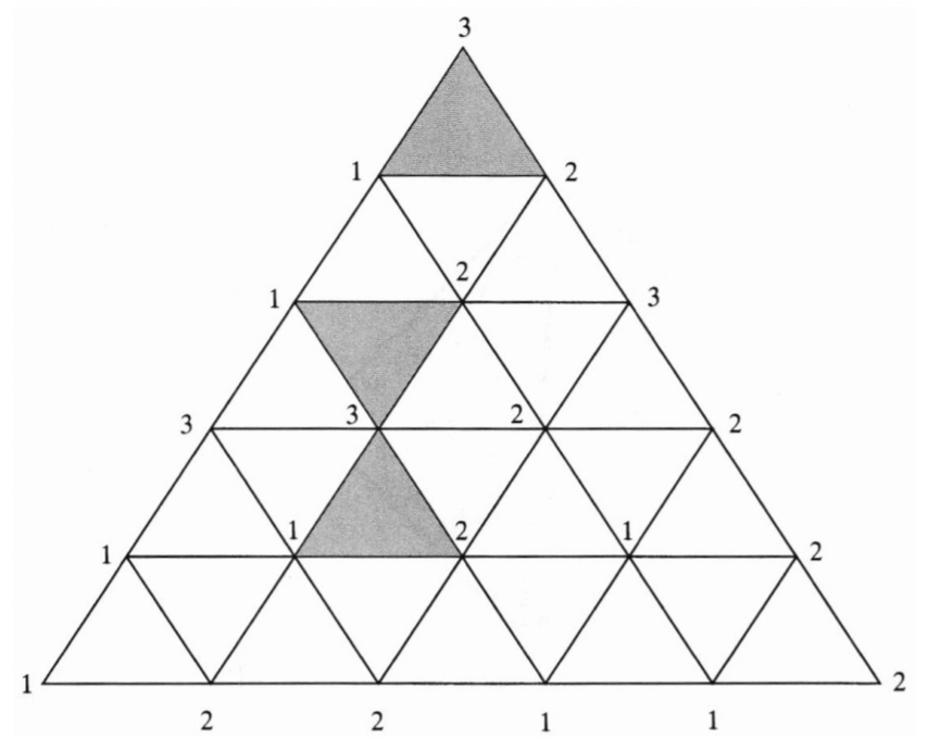
Refer to caption — Figure 1: Triangle T consisting of the union of multiple elementary triangles (from (citeS99)

We then create rules for labeling each labeling all of the vertices in $T$ as follows:

1.

all of the main vertices of $T$ (that is, the vertices of the main largest triangle) have different labels,
2.

the label of a vertex along any edge of $T$ matches the label of one of the main vertices spanning that edge, and
3.

labels in the interior of $T$ are arbitrary

We call any vertex labeling of $T$ that follows the conditions above a Sperner labeling.

Sperner’s Lemma for Triangles: Any Sperner-labelled triangulation of $T$ must contain an odd number of elementary triangles possessing all labels; in particular, there is at least one.

Now, we define an $n$ -simplex as an $n$ -dimensional "tetrahedron", or a convex hulll of $n+1$ affinely independent points in $\mathbb{R}^{m}$ , where $m\geq n$ . These points form the vertices of the simplex, and a $k$ -face of the $n$ -simplex is the $k$ -simplex formed by the span of anysubset of $k+1$ vertices. A triangulation of an $n$ -simplex $S$ is a collection of distinct smaller $n$ -simplices whose union is $S$ , with the property that any two of them intersect in a face commmon to both, or not at all. These smaller $n$ -simplices are called elementary simplices, and their vertices are called vertices of the triangulation.
Any face spanned by $n$ of the $n+1$ vertices of $S$ is called a facet. The number of facets that $S$ contains is $n+1$ , and we label them by $1,2,...,n+1.$ Given a triangulation of $S$ we consider a labelling that obeys the following rules:

1.

each vertex is labelled by one of the facet numbers in such a way that on the boundary of $S,$ none of the vertices on facet $j$ is labeled $j$ , and
2.

the interior vertices can be labeled by any of the facet numbers.

The labeling described above is called a Sperner labelling of an n-simplex, and an example of such a labeling when $n=3$ is shown in Figure 2.

Sperner’s Lemma: Any Sperner-labeled triangulation of an $n$ -simplex must contain an odd number fully labelled elementary $n$ -simplices. In particular, there is at least one.

The proof for the two lemmas above are described in detail in (citeS99) and involve induction.

Now, we give the following proof:

Claim: In a fisher market where all items are divisible, a CE always exists.
Proof: Consider a fisher market with a set of $n$ buyers $\mathcal{N}=[n]$ and a set of $m$ goods $\mathcal{M}=[m]$ . We assume that quantities are normalized, so for all $j\in\mathcal{M}$ , $C_{j}=1$ , and the budgets for all agents are normalized so that their sum is $1,$ meaning that for all $i\in\mathcal{N}$ , $\sum_{i}B_{i}=1.$ Moreover, we also assume that all products are good, meaning that an agent always strictly prefers to have one more of each product if they can afford it; this means that $u_{i,j}>0$ for each agent $i$ and good $j.$ $i\in\mathcal{N},j\in\mathcal{M}$ .

Now, we consider a standard simplex with $m-1$ vertices

\displaystyle\Delta^{m-1}=\bigg\{(x_{1},...,x_{m})\in\mathbb{R}^{m}\bigg|\sum_{i=1}^{m}x_{i}=1\text{ and }x_{i}\geq 0\text{ }\forall i\in\{1,...,m\}\bigg\}

We see that each point in $\Delta^{m-1}$ corresponds to a price-vector, where the sum of all prices is $1$ , meaning that the price of all goods together is $1.$
We now define the demanded set of a buyer $i$ as the set of affordable bundles that maximize the buyer’s utility among all affordable bundles given a price vector $\mathbf{p}$ , meaning that

\displaystyle\text{Demand}_{i}(\mathbf{p})=\arg\max_{\mathbf{x}_{i}:\mathbf{p}^{T}\mathbf{x}_{i}\leq B_{i}}u_{i}(\mathbf{x}_{i}),

where $\mathbf{x}_{i}$ is the bundle assigned to buyer $i$ , and

\displaystyle\mathbf{p}^{T}\mathbf{x}_{i}=\sum_{j=1}^{m}p_{j}x_{ij}.

For each price vector $\mathbf{p}\in\Delta^{m-1},$ we can find a demanded set for each agent and then calculate the sum of all demanded sets to find the total price of this aggregate demand. Since $\mathbf{p}^{T}\mathbf{x}_{i}\leq B_{i}$ for all $i\in\mathcal{N}$ , and $\sum_{i=1}^{n}B_{i}=1$ , this implies that $\sum_{i=1}^{n}\mathbf{p}^{T}\mathbf{x}_{i}\leq 1.$ Hence, for each $\mathbf{p}$ , there is at least one good for which the total demand is at most $1.$ We can then call this good an "expensive good" in $\mathbf{p}.$
We then triangulate the $m-1$ -vertex simplex, and go on to label each triangulation vertex $\mathbf{p}_{v}$ with an index of an arbitrary expensive product in $\mathbf{p}_{v}.$ We then see that in each of the facets of the simplex, some products cost $0.$ However, since $u_{ij}>0$ for all agents $i$ and goods $j$ , the demand of each agent for a product that costs $0$ is always $1;$ this implies that a product which costs $0$ can never be considered expensive. Note that this satisfies condition $1$ of a Sperner labeling of an $n$ -simplex.
We then know from Sperner’s Lemma that there exists an elementary simplex whose vertices are labeled with $m$ different labels. By repeatedly triangulating in a repeatefly finer fashion, we converge at a single price vector $\mathbf{p}^{*}$ , in which all products are expensive, meaning that the aggregate demand for every product is at most $1.$ Since the sum of all budgets is $1$ , the aggregate demand for every product in $\mathbf{p}^{*}$ becomes exactly $1.$ Therefore, $\mathbf{p}^{*}$ is a vector of market-clearing prices. $\blacksquare$

Although Sperner’s lemma can be used to find a CE, it is very computationally inefficient, and there are more efficient computational methods.

3.1.2 Vazirani’s Algorithm

Recall the KKT conditions discussed in Ssection 2.3. Note that one can derive that an optimal solution to the convex program above must satisfy the market clearing conditions.

Moreover, the Eisenberg-Gale program helps prove the following basic properties of equilibria for the linear case of Fisher’s market:

•

If each good has a potential buyer, equilibrium exists
•

The set of equilibium allocations is convex
•

Equilibium utilities and prices are unique
•

If all $u_{ij}$ ’s and $B_{i}$ ’s are rational, then equilibrium allocations and prices are also rational. Moreover, they can be written using polynomially many bits in the length of the instance.

In fact, the Eisenberg-Gale convex program is not only specific to Fisher Markets with linear utilities, but can be used to analyse the equilibrium state of an entire family of markets including but not limited to network flow markets, markets with Leontief utilities (citeCV04), scalable utilities (citeE61), homothetic utilities with productions (citeJVY05). The reader can refer to these papers for more in-depth expositions.

The algorithms that are often presented in literature enforce certain KKT conditions and relax others. It is easy to see that the equilibrium conditions for the Fisher Model are equivalent to the equilibrium conditions as defined for the Eisenberg Gale markets. One surprising property of Eisenberg-Gale program is that despite its non-linearity, it always has a rational solution if all the parameters in the instance are rational.

Vazirani (citeV07) provides a weakly polynomial-time algorithm for finding equilibrium prices and allocation for Fisher markets employing linear utilities by using primal-dual schema.It uses the assumption that each good as a potential buyer, meaning that the buyer derives positive utility from that good. Because of this assumption, it can be proven that market-clearing prices exist and are unique based on the Eisenberg-Gale program described in the previous section. The existence of such prices also follows from Sperner’s lemma, as descirbed in the previous sub-section.

Vazirani’s algorithm sketch involves the construction of a flow network in which the capacity of each edge represents the total money "flowing" through the edge. An example is shown in Figure 3. We can see that we have a source node $s,$ a node for each product, a node for each buyer, and a sink node $t.$ Note that there exists an edge from $S$ to each good $j$ with capacity $p_{j}$ , and that there exists an edge from a product $j$ to a buyer $i$ with infinite capacity if and only if the buyer likes the product, ie., $(j,i)$ is in the network if and only if $\frac{u_{ij}}{p_{j}}\geq\max_{k\in\mathcal{M}}\{u_{ik}/p_{k}\}$ . Moreover, note that there is an edge from each buyer to $t$ with capacity $B_{i}.$ $\mathcal{M}$ is the set of nodes that $s$ connects to, or the goods, and $\mathcal{N}$ is the set of nodes that connect to $t$ , or the buyers.
Lemma: Prices $\mathbf{p}$ are equilibrium prices if and only if in the network the two cuts $(s,\mathcal{M}\cup\mathcal{N}\cup t)$ and $(s\cup\mathcal{M}\cup\mathcal{N},t)$ are min-cuts. Allocations corresponding to any max-flow are equilibrium allocations.

Vazirani’s algorithm sketch is outlined as follows: (i) Start with low prices that are guaranteed to be below the equilibrium price for each good, and (ii) raise prices iteratively and reduce surplus money that buyers have. Once the surplus vanishes, the algorithm terminates and the resulting prices are equilibrium prices.
Two concerns for this algorithm are ensuring that the equilibrium price of no good is exceeded and that the surplus money of buyers reduces fast enough so the algorithm terminates in polynomial time. These details are quite involved, so they will be omitted for this project; however, they are discussed further in (citeV07). The full algorithm runs in weakly polynomial time. Specifically, the algorithm runs in $O((n+m)^{8}\log(u_{max})+(n+m)^{7}\log B_{max})$ time, where $u_{max}$ is the maximum utility and $B_{max}$ is the maximum budget. The runtime analysis is also quite involved, and thus will also be omitted.

Figure 3: The flow network constructed by the algorithm.

\mathcal{M}

consists of the nodes 1-4 on the left, and

\mathcal{N}

consists of nodes 1-3 on the right

In addition to this algorithm, Orlin (citeO10) gave an improved algorithm that runs in strongly polynomial time, with run-time $O((m+n)^{4}\log(m+n))$ .

3.2 Fisher Markets with Indivisible Items

Thus far in our discussion of Fisher markets we have assumed that all goods were divisible; that is, we are allowed to allocate to agents possibly fractional amounts of goods. In real-world scenarios, however, this is not exactly the case; what does it mean to allocate ‘one-fourth’ of a computer to a computer buyer?

Consequently, researchers have studied a variant of the usual Fisher market, but with indivisible items. Sometimes the term discrete Fisher market is used to refer to such markets. Note that when we study indivisible items, we can suppose without loss of generality that the number of each good on the market is integral.

In this section, we will provide a survey of some important and remarkable results from the study of Fisher markets with indivisible items.

First, we shall note that a competitive equilibrium is not always guaranteed to exist in a Fisher market with indivisible goods. In particular, (citeDPS03) showed in 2003 that in such a market, the problem of determining whether a competitive equilibrium exists is NP-hard, even in the simple case where there are three agents, each with a (textitlinear) utility function. However, the authors had demonstrated that there exists a polynomial time algorithm that finds a so-called “ $\epsilon$ -approximate equilibrium,” viz. an allocation $\{x_{i,j}\}$ such that for each good $j$ ,

(1-\epsilon)C_{j}\leq\sum_{i\in\mathcal{N}}x_{i,j}\leq C_{j}.

In this case, the market is said to clear “ $\epsilon$ -approximately,” i.e. at least $1-\epsilon$ of each good is allocated to the buyers. The algorithm that (citeDPS03) presents operates in time $O((n^{2}\log(\max_{j}C_{j})/\epsilon)^{2m})$ , which turns out to be polynomial in the size of the input.

A more stringent variant of this problem arises in the case when all buyers are assumed to have an equal budget. Without loss of generality, it can be assumed that each buyer has unit budget, as long as the prices and quantities of goods are scaled appropriately. The problem of determining whether a competitive equilibrium exists in such a market is called the competitive equilibrium with equal incomes (CEEI) problem.

In 2015, (citeA15) showed that the CEEI problem is strongly NP-hard in general. Moreover, the author proves that CEEI is weakly NP-hard in the case of just two buyers. To do this, the author constructs a reduction from this special case of CEEI to a more familiar weakly NP-complete $2$ -partitioning problem: Given a multiset $M$ of $m$ positive integers with sum $2C$ , is there a partition of $S$ such that the sum of the integers in each set is $C$ ?

Further, (citeA15) shows that in the case of $n$ buyers and $3n$ , a reduction from the $3$ -partitioning problem gives that the general CEEI problem is strongly NP-hard. Finally, (citeA15) also considers yet another variant of the CEEI-problem, called CEEI-FRAC, which allows for fractional allocations provided that the maximum amount of a good $j$ that can be assigned to a buyer $i$ is

	$\displaystyle x_{i,j}\in\left\{\{y_{i,j}\}:\{y_{i,j}\}\text{ is valid fractional allocation and }y_{i,j}\in Y_{i,j}\right\},$
	$\displaystyle\text{where each }Y_{i,j}=\arg\max\left\{u_{i,j}(y_{i,j}):\sum_{j\in\mathcal{M}}y_{i,j}p_{j}\leq 1\right\},$

and showing that CEEI-FRAC, surprisingly, is in NP.

Another fascinating version of the CEEI problem was studied by (citeB11) in 2011, where we consider an “approximate-CEEI” problem where a market approximated clears, buyers are only required to have approximately equal, and each buyer has an inherent preference relation over all feasible bundles of goods. Indeed, this A-CEEI problem can be thought of as one of the most general forms of the CEEI problem. (citeB11) demonstrates that an approximate competitive equilibrium always exists for some small error tolerance $\epsilon$ , and also shows that such an approximate can be made “strategyproof. This is to say, no buyers have an incentive to hide or lie about their personal preference relations.

Interestingly, (citeB11)’s work can be applied to the study of the effects that certain modern algorithms have that are not strategyproof; one such example is the course scheduling system at the Wharton School of Business, which apparently suffered from various flaws related to student incentives.

4 Research Direction

So far in our study of Fisher markets with divisible goods, we made a number of important assumptions. For one, we had assumed that buyers’ utilities were generally independent of one another. That is to say, how much utility buyer $i$ derives from a good is not affected by how much utility buyer $j$ derives that from same good, or by how much buyer $j$ ends up owning that good.

However, in certain real-world markets, this assumption might not be applicable. In a seminal paper from 1950, (citesnob) defines the snob effect as the apparent micro-economic phenomenon where a buyer may have a higher demand for goods that he or she perceives to be somehow ‘unique.’ For instance, among a pool of buyers of a particular class of luxury goods (say, Gucci sneakers), the utility that a buyer derives from a good can be diminished if too many other buyers in the pool own that same good.

Let us recall that $\mathcal{M}$ and $\mathcal{N}$ denote sets of goods and buyers. For each good $j\in\mathcal{M}$ , again we associate a price $p_{j}$ and an amount $C_{j}$ of that good in existence. And once more, we let $x_{i,1},\dots,x_{i,m}$ denote an allocation of each good to a buyer $i$ .

As a first pass, we can consider the following utility function for a single buyer $i$ , which is nonlinear:

u_{i}(x_{i,1},\dots,x_{i,m})=\sum_{j\in\mathcal{M}}\frac{x_{i,j}}{\sum_{k\in\mathcal{N}}x_{k,j}}.

Here we assume that the $j$ -th term in the overall summation if zero if good $j$ was not allocated to any buyers (i.e. if the denominator is zero).

Such a utility function is able to crudely represent the snob effect – the utility for buyer $i$ for a given bundle of goods decreases if too many other buyers also own a substantial portion of the goods that buyer $i$ owns.

However, this definition fails to account for an a priori preference that a buyer might have for a certain good; to account for this in conjunction with the snob effect, let us reuse the notation $v_{i,j}$ to refer to the utility that buyer $i$ derives from obtaining a unit of good $j$ , absent any information about the other buyers. Moreover, for each buyer $i$ we specify a sensitivity $\alpha_{i}$ , which represents the degree to which this buyer is sensitive to the snob effect.

Then, we can define the following modified utility function, which is still nonlinear:

U_{i}(x_{i,1},\dots,x_{i,m},v_{i,1},\dots,v_{i,m})=\sum_{j\in\mathcal{M}}x_{i,j}v_{i,j}\Big(\frac{x_{i,j}}{\sum_{k\in\mathcal{N}}x_{k,j}}\Big)^{\alpha_{i}}.

Note that if $\alpha_{i}=0$ for each buyer $i$ , then the utility function of buyer $i$ reduces to the linear case, so we will assume that $\alpha_{i}>0$ for some $i$ .

Our objective is given by

		$\displaystyle\text{maximize }\sum_{i\in\mathcal{N}}U_{i}$
	$\displaystyle\text{subject to }\qquad U_{i}$	$\displaystyle=\sum_{j\in\mathcal{M}}x_{i,j}v_{i,j}\Big(\frac{x_{i,j}}{\sum_{k\in\mathcal{N}}x_{k,j}}\Big)^{\alpha_{i}}$
	$\displaystyle x_{i,j}$	$\displaystyle\geq 0\quad\text{for each buyer }i\text{ and good }j$
	$\displaystyle\sum_{j\in\mathcal{M}}x_{i,j}p_{j}$	$\displaystyle\leq B_{i}\quad\text{for each buyer }i$
	$\displaystyle\sum_{i\in\mathcal{N}}x_{i,j}$	$\displaystyle\leq C_{j}\quad\text{for each good }j.$

We shall prove a simple case with one good and two buyers, with each buyer having sensitivity $1$ to the snob effect. Assume that the good costs unit price and has unit amount available. Also assume that each buyer has unit budget and the same a priori preference for the good.

Theorem: In such a market, the optimal allocation is found by allocating the entirety of one good to a single buyer and leaving none for the other.

Proof: Denote the allocation of the good to the two buyers as $x$ and $y$ , and denote the common a priori utility of the good as $u$ .

As such, our objective is given by:

		$\displaystyle\text{maximize }U_{1}+U_{2}$
	$\displaystyle\text{subject to }\qquad U_{1}$	$\displaystyle=\frac{ux^{2}}{x+y};\quad U_{2}=\frac{uy^{2}}{x+y}$
	$\displaystyle x,y$	$\displaystyle\geq 0\qquad\text{(nonnegative allocation)}$
	$\displaystyle x,y$	$\displaystyle\leq 1\qquad\text{(price constraint)}$
	$\displaystyle x+y$	$\displaystyle\leq 1\qquad\text{(available quantity of the good)}.$

We can rewrite the objective via

	$\displaystyle\max U_{1}+U_{2}$	$\displaystyle=\max u\left(\frac{ux^{2}}{x+y}+\frac{uy^{2}}{x+y}\right)$
		$\displaystyle=\max\frac{x^{2}+y^{2}}{x+y},$

where $x$ and $y$ clearly lie on the $2$ -simplex. Note that $(x^{2}+y^{2})/(x+y)$ have no critical points on the interior of the $2$ -simplex, and its values on the lines $x=0$ and $y=0$ strictly increase, reaching a common maximum value of $1$ at $(0,1)$ and $(1,0)$ . Moreover, on the boundary $x+y=1$ we also have that the maximum values are attained at those two points. Thus, the maximum value is attained either at $(0,1)$ or $(1,0)$ , so we conclude that the optimal allocation is found by allocating all of one good to a single buyer and none to the other buyer. $\blacksquare$

We would then want to explore whether these sorts of markets do generally contain market-clearing prices, and if so, how to efficiently calculate them.

5 Conclusion

Matching markets are extremely important models which capture interesting economic phenomena. We detailed the preliminaries of Fisher markets and Gale-Eisenberg markets, and we provided a literature review of the state of computing CE for Fisher markets with divisible and indivisible items. Moreover, we provided a research direction which aims to investigate fisher markets where utilities follow the snob effect in hopes of creating additional market models which capture wider phenomena not currently investigated in the literature.

References

[1] Alvin E. Roth, Tayfun Sonmez, and M. Utku Unver. Kidney Exchange. The Quarterly Journal of Economics, 119(2):457-488, 2004.

[2] Alvin E Roth and Marilda Sotomayor. A study in game-theoretic modeling and analysis. Econometric Society Monographs, 18, $1990$ .

[3] Tayfun Sonmez and M. Utku Unver. Chapter $17$ : Matching, Allocation and Exchange of Discrete Resources. Volume 1 of Handbook of Social Economics, pages $781-852$ . North-Holland, $2011$ .

[4] Yishay Mansour. Advanced topics in machine learning and algorithmic game theory, March $2016$ .

[5] Kamal Jain and Vijay V. Vazirani. Eisenberg-Gale Markets : Algorithms and Game-Theoretic Properties. Games and Economic Behaviour, $70(1):84-106,2010$ . Special Issue in Honor of Ehud Kalai.

[6]Herbert E. Scarf. The core of an $n$ -person game. Econometrica, $35(1):50-69,1967$ .

[7] Francis Edward Su. Rental Harmony: Sperner’s Lemma in Fair Division. The American Mathematical Monthly, $106(10):930-942,1999$ .

[8] Bruno Codenotti and Kasturi Varadarajan. Efficient Computation of Equilibrium Prices for Markets with Leontief Utilities. Volume $3142$ , Pages $371-382$ , $072004$ .

[9] E. Eisenberg. Aggregation of Utility Functions. Management Science, $7(4):337-350$ , July $1961$ .

[10] Kamal Jain, Vijay Vazirani and Yinyu Ye. Market Equilibria for Homothetic, Quasi-Concave Utilities and Economies of Scale in Production. Pages $63-71$ , $01-2005$ .

[11] Vijay V. Vazirani. Combinatorial Algorithms for Market Equilibria. Algorithmic Game Theory, Pages $103-134,2007$ .

[12] James B. Orlin. Improved Algorithms for Computing Fisher’s Market Clearing Prices: Computing Fisher’s Market Clearing Prices. In Proceedings of the Forty-Second ACM Symposium on Theory of Computing, STOC’10, page $291-300$ , New York. NY, USA, $2010$ . Association for Computing Machinery.

[13] Xiaotie Deng, Christos Papadimitriou Shmuel Safra. On the Complexity of Price Equilibria. Journal of Computer and System Sciences, $67(2):311-324,2003$ . Special Issue on STOC $2002$ .

[14] Haris Aziz. Competitive Equilibrium with Equal Incomes for Allocation of Indivisible Objects. Operations Research Letters, $43(6):622-624,2015$ .

[15] Eric Budish. The combinatorial Assignment Problem: Approximate Competitive Equilibrium from Equal Incomes. Journal of Political Economy, $119(6):1061-1103,2011$ .

[16] H. Leibenstein. Bandwagon, Snob, and Veblen Effects in the Theory of Consumers’ Demand. The Quarterly Journal of Economics., $64(2):183-207,051950$ .