Adaptive Bayesian Sum of Trees Model for Covariate Dependent Spectral Analysis

The covariate-dependent power spectrum introduced in Section 2 can be approximated by piecewise stationary processes via partitioning the covariate space into approximately stationary blocks. Piecewise stationary approximations of the power spectrum have been well-studied within the context of nonstationary time series analysis (Adak 1998; Rosen et al. 2012), where time series are divided into approximately stationary intervals for time-dependent spectral analysis. Bruce et al. 2018 introduced a time- and covariate-based piecewise stationary approximation for time- and covariate-dependent spectral analysis using a two-dimensional grid.

However, directly extending a two-dimensional grid to higher dimensions in order to accommodate multiple covariates can easily lead to over-parameterization and undue computational complexity. Tree-based approaches represent a more flexible and parsimonious alternative for partitioning multiple covariates. A grid-based partition tends to produce a finer partition than is necessary, since partition points for each covariate do not depend on the other covariate. This results in less efficient information sharing across series with similar covariates and less accurate estimation. Conversely, if the true partition does have a grid structure, a tree-based model can still well-approximate the partition and is thus preferable.

For tree-based piecewise stationary approximation, each terminal node is defined through a collection of splitting rules corresponding to the tree structure and represents an approximately stationary region of the covariate space. Suppose a tree $U$ has $B$ terminal nodes. The corresponding piecewise stationary approximation is

where $X_{t}^{(b)}$ is stationary process with power spectrum $f_{b}(\nu)=|A_{b}(\nu)|^{2}$ corresponding to the $b$th terminal node, and $\delta$ is a function that identifies terminal node membership for each observation based on covariates such that $\delta(\boldsymbol{\omega}_{\ell};U,b)=1$ if the $\ell$th observation falls into the $b$th terminal node and $\delta(\boldsymbol{\omega}_{\ell};U,b)=0$ otherwise.

We now introduce an estimator for local power spectra within terminal nodes of the tree. Let $N=\lfloor T/2\rfloor-1$ and $\nu_{k}=k/T$ for $k=1,\ldots,N$ be the Fourier frequencies. The periodogram estimator of the power spectrum for the $\ell$th time series is $I_{\ell}(\nu_{k})=\frac{1}{T}\left|\sum_{t=1}^{T}X_{\ell t}\exp(-2\pi i\nu_{k}t)\right|^{2}.$ The Whittle likelihood (Whittle 1952), derived from the large sample distribution of the periodogram, can then be used to approximate the overall likelihood for the tree as a product of individual likelihoods, assuming $T$ is sufficiently large,

Log power spectra within each terminal node $\log f_{b}(\nu)$ are modeled using a Bayesian penalized linear spline model (Rosen et al. 2012)

where the functions $\cos(2\pi s\nu)$ are the Demmler–Reinsch basis functions for periodic even splines observed on an evenly spaced grid (i.e. the Fourier frequencies) (Schwarz and Krivobokova 2016, Section 3). Only the first $S<N$ basis functions are used to provide a low-rank approximation to the full linear smoothing spline (Eubank 1999). In order to achieve good computational efficiency without sacrificing estimation accuracy (Krafty et al. 2017), $S=7$ basis functions are used for subsequent simulations and real data analyses, which provide good empirical performance. Gaussian priors are assumed such that $\alpha_{b}\sim N(0,\sigma_{\alpha}^{2})$ where $\sigma_{\alpha}^{2}$ is a large constant value, and $\boldsymbol{\beta}^{(b)}=(\beta_{1}^{(b)},\ldots,\beta_{S}^{(b)})^{\prime}\sim N(0,\tau_{b}^{2}\boldsymbol{D}_{S})$, where $\boldsymbol{D_{S}}=\text{diag}(\{\sqrt{2}\pi s\}^{-2})$. $\tau_{b}^{2}$ is a smoothing parameter that controls the roughness of the log spectrum. The scaling for the smoothing parameter, $\{\sqrt{2}\pi s\}^{-2}$, provides regularization of the integrated squared first derivative of the log power spectrum (Li and Krafty 2019). A half-t prior is placed on $\tau_{b}$ (Gelman 2006) to complete the Bayesian model specification. We follow Wand et al. 2011 and express the half-t distribution as a scale mixture of inverse gamma distributions for efficient sampling. A two-step MCMC sampling scheme for $\alpha_{b}$, $\boldsymbol{\beta}^{(b)}$, and $\tau_{b}$ following Rosen et al. 2012 is presented below.

1. 1.

   Let $\boldsymbol{Z}_{b}$ be a $N\times S$ matrix of basis functions for $b$th terminal node such that $\{Z_{b}\}_{k,s}=\cos(2\pi s\nu_{k})$. Given $\tau_{b}$, basis functions $\boldsymbol{Z}_{b}$, and periodogram ordinates $\boldsymbol{I}_{\ell}(\nu)=\{I_{\ell}(\nu_{1}),$
   $I_{\ell}(\nu_{2}),\ldots,I_{\ell}(\nu_{N})\}$ for $l=1,\ldots,L$, $\alpha_{b}$ and $\boldsymbol{\beta}^{(b)}$ are sampled jointly in a Metropolis-Hastings (M-H) step from

   $$\begin{split}p(\alpha_{b},\boldsymbol{\beta}^{(b)}|\tau_{b}^{2},\boldsymbol{I}_{\ell}(\nu),\boldsymbol{Z}_{b})&\propto\exp\Big\{-\sum_{\ell=1}^{L}\sum_{k=1}^{N}[\alpha_{b}+\mathbf{z}_{bk}^{\prime}\boldsymbol{\beta}^{(b)}+\exp\big(\log I_{\ell}(\nu_{k})\\ &-\alpha_{b}-\mathbf{z}_{bk}^{\prime}\boldsymbol{\beta}^{(b)}\big)]-\frac{\alpha_{b}}{2\sigma_{a}^{2}}-\frac{1}{2\tau_{b}^{2}}\boldsymbol{\beta}^{(b)^{\prime}}\boldsymbol{D}_{S}^{-1}\boldsymbol{\beta}^{(b)}\Big\}.\end{split}$$

   (3)

2. 2.

   By representing the half-t prior as a scale mixture of inverse gamma distributions (Wand et al. 2011), we obtain draws of $\tau_{b}$ from its full conditional distribution by sampling from

   $$(a_{b}|\tau_{b}^{2})\sim\text{IG}\Big(\frac{\xi_{\tau}+1}{2},\frac{\xi_{\tau}}{\tau_{b}^{2}}+\frac{1}{A_{\tau}^{2}}\Big),$$

   (4)

   and

   $$(\tau_{b}^{2}|a_{b},\boldsymbol{\beta}^{(b)})\sim\text{IG}\Big(\frac{\xi_{\tau}+S+1}{2},\frac{\boldsymbol{\beta}^{(b)^{\prime}}\boldsymbol{\beta}^{(b)}}{2}+\frac{\xi_{\tau}}{a_{b}}\Big)$$

   (5)

   where $a_{b}$ is a latent variable, and $\xi_{\tau}$ and $A_{\tau}^{2}$ are fixed hyperparameters of the inverse gamma distribution.

Poor mixing of single tree models has been noted in many applications such that the MCMC algorithm becomes stuck in subsets of the covariate space representing local optima and cannot efficiently traverse the entire parameter space (Wu et al. 2007). This can happen when single tree models grow very large in an effort to approximate more complex relationships, thus restricting possible modifications due to low sample size and an abundance of other splits. We follow Chipman et al. 2010 in developing a Bayesian sum of trees formulation to relieve this problem by constructing many shallow trees as “weak learners” for estimation.

Let $M$ be the number of trees. A sum of trees model for the log power spectrum is then constructed as

where $U_{j}$ represents the $j$th tree that has $B_{j}$ terminal nodes for $j=1,\ldots,M$. Model specification for local power spectra $\log f_{bj}(\nu)$ within each tree then follows directly from the specification for the single tree model introduced in Section 3.2.

Let $\Phi_{j}=\{\log f_{1j}(\nu),\ldots,\log f_{B_{j}j}(\nu)\}$ be the collection of log power spectra across terminal nodes for the $j$th tree. To complete the Bayesian model specification, priors are imposed on $U_{j}$ and $\Phi_{j}$ in order to allow the trees to be random and fit from the data. Assuming independence across terminal node parameters and trees a priori, priors can be specified as

where

The priors for $\Phi_{j}|U_{j}$ then correspond to the priors of $\alpha_{b}$, $\boldsymbol{\beta}^{(b)}$ and $\tau_{b}$ for the local power spectrum estimator introduced in Section 3.2. For the priors on the tree structure $U_{j}$, three probabilities need to be considered.

1. 1.

   The probability of a node to be split is defined as $\Pr(\text{SPLIT})=\gamma(1+d)^{-\theta}$, where $\gamma\in(0,1),\ \theta\in[0,\infty)$ and $d=0,1,\ldots$ is the depth of a given node. This prior is a regularization of the tree depth to encourage each tree to be shallow. We set $\gamma=0.95$ and $\theta=2$ following Chipman et al. 2010. Ročková and Saha 2019 propose a minor modification $\Pr(\text{SPLIT})\propto\gamma^{d}$ for some $0\leq\gamma<1/2$ to achieve the optimal posterior convergence rate, which can also be adopted within the proposed framework.

2. 2.

   The probability of selecting the $p$th covariate for splitting is denoted as $s_{p}$ for $p=1,\ldots,P$. The proposed model allows for two possible prior specifications: a uniform prior, $s_{p}=P^{-1}$, such that all covariates have the same probability to be selected, and a sparsity-inducing Dirichlet prior $(s_{1},\ldots,s_{P})\sim\mathcal{D}\Big(\frac{\sigma}{P},\ldots,\frac{\sigma}{P}\Big)$ (Linero 2018). For the Dirichlet prior, $\sigma$ determines the degree of sparsity and Linero 2018 offer multiple approaches for modeling this parameter. We set $\sigma=1$ as suggested by Linero 2018 for computational convenience.

3. 3.

   The probability of selecting a particular cutpoint for a given covariate is uniform across all cutpoints. A uniform prior is also desirable as it is invariant for monotone transformations of the covariate (Chipman et al. 2010). For continuous, discrete, and ordinal covariates, cutpoints are selected from a fixed number of evenly spaced points over the range of possible values. For categorical covariates without an intrinsic ordering, a cutpoint represents a particular mapping of categories to the left and right child nodes created by the split. A categorical variable with $q$ categories then has $2^{q}-2$ cutpoints that can be selected.

It is important to note that each tree is capturing particular features of the covariate-dependent power spectrum and also depends on the features captured by other trees. While this provides considerable flexibility and adaptive estimation, it presents significant computational challenges in estimating the trees. Following Chipman et al. 2010, we develop a Bayesian backfitting MCMC algorithm for proposing and evaluating modifications to each tree sequentially.

For the $j$th tree, the posterior distribution $p\big((U_{1},\Phi_{1}),...,(U_{M},\Phi_{M})|\boldsymbol{I}_{1}(\nu_{k}),\ldots,\boldsymbol{I}_{L}(\nu_{k})\big)$ can be sampled through $M$ successive draws from $p\big((U_{j},\Phi_{j})|U_{-j},\Phi_{-j},\boldsymbol{I}_{1}(\nu_{k}),\ldots,\boldsymbol{I}_{L}(\nu_{k})\big)$ where $U_{-j}$ is the set of all trees except $U_{j}$, and $\Phi_{-j}$ is defined similarly. Observe that the conditional distribution $p\big((U_{j},\Phi_{j})|U_{-j},\Phi_{-j},\boldsymbol{I}_{1}(\nu_{k}),\ldots,\boldsymbol{I}_{L}(\nu_{k})\big)$ depends on $\big(U_{-j},\Phi_{-j},\boldsymbol{I}_{1}(\nu_{k}),$
$\boldsymbol{I}_{2}(\nu_{k}),\ldots,\boldsymbol{I}_{L}(\nu_{k})\big)$ only through

where $\mathbf{R}_{\ell j}(\nu_{k})$ is the residual of the log periodogram after removing the fit from the sum of trees across all trees except for the $j$th tree. Therefore, drawing from the posterior distribution equates to $M$ successive draws from $p\big((U_{j},\Phi_{j})|\mathbf{R}_{1j}(\nu_{k}),\ldots,\mathbf{R}_{Lj}(\nu_{k})\big)$. Hence, the local power spectrum estimator for the $j$th tree is then fit by replacing $\log\boldsymbol{I}_{\ell}(\nu_{k})$ with $\mathbf{R}_{\ell j}(\nu_{k})$ in Equation (1) and Equation (3).

To sample new tree structures, a reversible-jump MCMC (RJMCMC) (Green 1995) procedure is developed to jointly propose and evaluate new draws of $U$ and $\Phi$ for each tree. The proposed modification takes the form of one of three possible moves: BIRTH, DEATH and CHANGE, with probabilities 0.25, 0.25 and 0.5 respectively. The BIRTH move grows the tree by splitting a terminal node into two child nodes, the DEATH move prunes the tree by dropping two terminal child nodes belonging to the same internal node, and the CHANGE move modifies the variable and cut point associated with an internal node with two terminal child nodes. New model parameters for the proposed tree modification are drawn, and the proposed tree modification is then accepted or rejected using a Metropolis–Hastings (M-H) step. Each tree is considered in turn for updating within each iteration. Draws using this RJMCMC sampling scheme are repeated and averaged over post burn-in draws to obtain the final estimator. Technical details for the RJMCMC sampling scheme are available in Web Appendix A.

1. 1.

   Abrupt+Smooth: Let $\boldsymbol{\omega}=(\omega_{1},\omega_{2})$ where $\omega_{1},\omega_{2}\stackrel{{\scriptstyle i.i.d.}}{{\sim}}U(0,1)$. An AR(1) process for the $\ell$th time series is specified as $x_{\ell t}=\phi_{\ell}x_{\ell t-1}+\epsilon_{\ell t},\;\epsilon_{\ell t}\sim N(0,1),$ where $\phi_{\ell}=-0.7+1.4\omega_{2}$ when $0\leq\omega_{1}<0.5$ and $\phi_{\ell}=0.9-1.8\omega_{2}$, when $0.5\leq\omega_{1}\leq 1$.

2. 2.

   AR-Friedman: Let $\boldsymbol{\omega}=(\omega_{1},\ldots,\omega_{5})$ where $\omega_{1},\ldots,\omega_{5}\stackrel{{\scriptstyle i.i.d.}}{{\sim}}U(0,1)$. An AR(1) process for the $\ell$th time series is specified as $x_{\ell t}=\phi_{\ell}x_{\ell t-1}+\epsilon_{\ell t},\;\epsilon_{\ell t}\sim N(0,1),$ where $\phi_{\ell}=0.5\sin(\pi\omega_{\ell 1}\omega_{\ell 2})-(\omega_{\ell 3}-0.5)^{2}+0.35\mathrm{sign}(\omega_{\ell 4}-0.5)-0.15\omega_{\ell 5}$.

3. 3.

   Adjusted-AdaptSPEC-X: Let $\boldsymbol{\omega}=(\omega_{1},\omega_{2})$, where $\omega_{1},\omega_{2}\stackrel{{\scriptstyle i.i.d.}}{{\sim}}U(0,1)$. Each covariate vector $\boldsymbol{\omega}$ is mapped to a latent variable $z_{\ell}\in\{1,2,3,4\}$. Figure 6 shows the mapping from $\boldsymbol{\omega}$ to $z$. An AR(2) process is then specified as $x_{\ell t}=\phi_{z_{\ell}1}x_{\ell t-1}+\phi_{z_{\ell}2}x_{\ell t-2}+\epsilon_{\ell t},\;\epsilon_{\ell t}\sim N(0,1),$ where the coefficients for the four latent region are defined as follows. If $z_{\ell}=1$, $(\phi_{z_{\ell}1},\phi_{z_{\ell}2})=(1.5,-0.75)$; if $z_{\ell}=2$, $(\phi_{z_{\ell}1},\phi_{z_{\ell}2})=(-0.8,0)$; if $z_{\ell}=3$, $(\phi_{z_{\ell}1},\phi_{z_{\ell}2})=(-1.5,-0.75)$; if $z_{\ell}=4$, $(\phi_{z_{\ell}1},\phi_{z_{\ell}2})=(0.2,0)$.

The first setting represents an AR(1) process in which the coefficient varies smoothly across one covariate and abruptly across another. The second setting contains complex linear and nonlinear covariate effects and interactions (Friedman 1991) adapted for time series data. The third setting represents an abruptly-changing process over two dimensions, similar to that of Bertolacci et al. 2019.

Hyperparameters are specified as $\sigma_{\alpha}^{2}=100$ for the prior variance of $\alpha_{b}$ in Equation (2) and $\xi_{\tau}=2$ and $A_{\tau}=10$ for the prior on $\tau_{b}$ in Equation (4) and Equation (5). We used $M=5$ trees for estimation, and different numbers ($L$) and lengths ($T$) of time series are considered. The MCMC procedure is run for a total of 10,000 iterations with the first 5,000 discarded as burn-in. In order to assess convergence, trace plots for summary measures of the mean squared residuals, estimated log power spectrum, and tree structures for all settings are available in the Web Appendix B. These diagnostics appear to show convergence after approximately 5,000 iterations across all settings.

Estimates of the covariate-dependent power spectrum for this run are presented in Figure 3 to visually illustrate the ability of the proposed method to capture abrupt and smooth changes in power spectra. The smooth change in the conditional power spectrum over $\omega_{2}$ is captured by averaging over the posterior distribution of tree structures, which contains many splits across the range of possible values of $\omega_{2}$. On the other hand, splits on $\omega_{1}$ are concentrated around the true abrupt change at $\omega_{1}=0.5$, and the posterior mean estimator of the conditional power spectrum over $\omega_{1}$ appropriately reflects the abrupt change in the conditional power spectrum.

To evaluate estimation accuracy, the mean and standard deviation of the mean squared error (MSE) is presented in Table 1 for 100 replications of all settings. For comparison, AdaptSPEC-X (Bertolacci et al. 2019) is also used to estimate the covariate-dependent power spectrum. It is important to note that AdaptSPEC-X allows for modeling of time- and covariate-varying power spectra with time-varying means, which is a more general setting than what is considered in this work. Accordingly, we implement a simplified version of the AdaptSPEC-X mixture model without the time-varying mean and power spectra components to enable more accurate comparisons. We applied $C=50$ mixture components to ensure sufficient flexibility in estimating covariate effects on power spectra.

These results show that both methods see improved estimation accuracy as the number ($L$) and length ($T$) of time series increase. However, the proposed method generally carries smaller MSEs than AdaptSPEC-X for comparable settings. This can be partially attributed to the presence of abrupt changes across one or more covariates in all settings, which are better captured by the proposed tree-based approach. To illustrate this point, Figure 2(b) shows the estimated power spectra for two simulated time series with similar covariate values separated by an abrupt change from the Adjusted-AdaptSPEC-X setting. As noted in Bertolacci et al. 2019, the thin-plate Gaussian process prior on the mixture weights, while flexible, is both smooth and stationary. Accordingly, the AdaptSPEC-X power spectrum estimates for these two time series are similar due to smoothing across similar covariate values induced by the thin-plate Gaussian process prior. On the other hand, the proposed Bayesian sum-of-trees model is able to accurately distinguish the abrupt change in the power spectra. Moreover, averaging over the posterior distribution of trees enables the proposed method to recover smooth changes well (Figure 3). Taken together, this results in superior estimation accuracy across all settings seen in Table 1.

Simulations were carried out on a Windows 10 machine with an 8-core Intel i7 3.6 GHz processor and 64 GB RAM using R version 4.0.3 (R Core Team 2021). The R code for implementing the proposed model is provided as a zip file in Supporting Information and is described in Web Appendix C. Computationally-intensive aspects of the methodology are written in C++ using RcppArmadillo (Eddelbuettel and Sanderson 2014) for more efficient computation and reduced run times. Replications were run in parallel across six cores. For the simulation settings considered herein, the mean run time for each tree update after burn-in ranges from 0.02 to 0.43 seconds, depending on the number ($L$) and length ($T$) of time series. The distribution of mean run times for each setting with different $L$ and $T$ and $M=5$ trees are visualized in the Web Appendix B.

While run times generally increase as the number and length of time series increase, length increases have a bigger impact on run times relative to increases in the number of time series. Increasing $T$ from 100 to 500 while holding $L$ constant increases mean run times by a multiple of approximately 3.5, while increasing $L$ from 100 to 500 while holding $T$ constant increases mean run times by a multiple of approximately 2.1. This is expected since the number of Fourier frequencies grows with the length of the series and increases both the number of terms being summed in the log Whittle likelihood and the dimension of the cosine basis used to approximate local log power spectra. However, increasing the number of time series does not change the number of Fourier frequencies and only requires adding more terms in the log Whittle likelihood and posterior distribution for the spline coefficients, which is less computationally expensive. See Equations (1)-(3) in Section 3.2 and sampling scheme details in the Web Appendix A for more details.

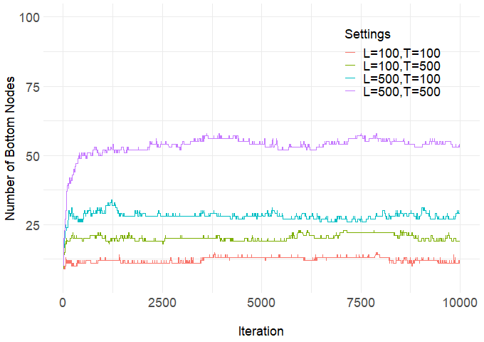
Tree size also plays an important role in determining run times for tree updates. Larger trees tend to have fewer time series belonging to each terminal node, which reduces computational burden and run times for evaluating modifications to a single terminal node. This is why the Adjusted-AdaptSPEC-X setting, which requires larger trees to recover the complex covariate effects, has faster mean run times compared to other settings. Additionally, tree size tends to increase as both $L$ and $T$ increase. For illustration, the Web Appendix B includes a plot of the total number of bottom nodes for different combinations of $L$ and $T$ for the AR-Friedman simulation setting. This can also help explain why run times grow more slowly in $L$ compared to $T$.

In order to demonstrate the capability of the proposed method in providing efficient variable selection by adapting to sparse covariate effects for high-dimensional covariates, we consider a modification to the AR-Friedman simulation setting introduced previously. The original covariate vector containing 5 important covariates is now extended to include 95 additional noise covariates independently drawn from a standard normal distribution. Variable selection efficiency can be investigated by assessing the estimated posterior probability for model inclusion of each covariate, which is the proportion of posterior draws where the covariate appears in at least one split rule for at least one tree. The estimated posterior probabilities for model inclusion for each of the 100 covariates using the uniform hyperprior and the sparsity-inducing Dirichlet prior for a single run of the proposed algorithm are shown in Web Appendix B. Both forms of the prior correctly estimate the posterior probabilities of model inclusion to be 1 for all 5 important variables, but the Dirichlet prior accurately achieves a sparser solution with the posterior probability of inclusion for the noise variables being much closer to 0. Specifically, the mean posterior probability of inclusion for noise variables using the uniform prior is 0.11 with a standard deviation of 0.1861, and the mean posterior probability of inclusion for noise variables using the Dirichlet prior is 0.01 with a standard deviation of 0.1026. For high-dimensional covariates in which only a few covariates are expected to be associated with the properties of the time series, the Dirichlet prior provides accurate selection of important covariates.

For the BIRTH move, the $b$th terminal node of the $j$th tree is selected to be split into two new child nodes. The proposed tree differs from the original tree only through the change from this terminal node to new child nodes. Therefore, the likelihood ratio becomes

where $b_{l}$ denotes left child node, $b_{r}$ is for the right child node, $n_{l}$ is the number of series corresponding to the proposed left child node, $n_{r}$ is the number of series corresponding to the proposed right child node, $\mathbf{R}_{b_{l}i}$ are residuals of the log periodogram ordinates for the $i$th series corresponding to the proposed left child node, and $\mathbf{R}_{b_{r}i}$ defined similarly for the proposed right child node. The likelihood within the terminal node is as shown in Equation (9). The tree structure ratio is expressed as

For the transition probability $q(U|U^{*})$ and $q(U^{*}|U)$, they can be expressed as

and

where $p(\text{GROW})=0.25$ and $p(\text{PRUNE})=0.25$ are the probability of BIRTH and DEATH move to be selected, and $n_{\text{internal}^{*}}$ is the total number of internal nodes that has two terminal child nodes. Thus, we can derive the transition ratio to be

Then, we follow Rosen et al. 2012 to draw the proposed terminal parameters $\boldsymbol{\beta}^{*}$, $\tau^{2*}$ and latent variable $a^{*}$. For $\tau^{2}$(a), let $\tau^{2}_{b}(a_{b})$ denote the current $\tau^{2}(a)$ for the $b$th terminal node and a uniform distribution is used to generate new parameters $\tau^{2*}_{b_{l}}(a^{*}_{b_{l}})$ and $\tau^{2*}_{b_{r}}(a^{*}_{b_{r}})$ for the left and right child. Specifically,

where $u_{\tau},u_{a}\sim U[0,1]$. For $\boldsymbol{\beta}$, an approximated normal distribution is proposed to generate the new parameters $\boldsymbol{\beta}^{*}_{b_{l}}$ and $\boldsymbol{\beta}^{*}_{b_{r}}$. Specifically, $(\boldsymbol{\beta}^{*}_{b^{*}}|\tau_{b^{*}}^{2*},U^{*},U,\Phi)\sim N(\boldsymbol{\beta}^{\text{max}}_{b},\boldsymbol{\Sigma}^{\text{max}}_{b})$, where

and

References

- Adak (1998) Adak, S. (1998). Time-dependent spectral analysis of nonstationary time series. Journal of the American Statistical Association 93, pp. 1488-1501.
- Apley and Zhu (2020) Apley, D. W. and Zhu, J. (2020). Visualizing the effects of predictor variables in black box supervised learning models. Journal of the Royal Statistical Society. Series B, Statistical Methodology 82, 1059–1086.
- Bertolacci et al. (2019) Bertolacci, M., Rosen, O., Cripps, E., and Cripps, S. (2019). AdaptSPEC-X: Covariate dependent spectral modeling of multiple nonstationary time series. ArXiv .
- Blattenberger and Fowles (2017) Blattenberger, G. and Fowles, R. (2017). Treed avalanche forecasting: Mitigating avalanche danger utilizing Bayesian additive regression trees. Journal of Forecasting 36, 165–180.
- Breiman (2001) Breiman, L. (2001). Random forests. Machine Learning 45, 5–32.
- Brenière and Bril (1988) Brenière, Y. and Bril, B. (1988). Why do children walk when falling down while adults fall down in walking? Comptes Rendus de l’Académie des Sciences. Série III, Sciences de la Vie 307, 617–22.
- Brillinger (2002) Brillinger, D. R. (2002). Time Series: Data Analysis and Theory. Philadelphia: SIAM.
- Bruce et al. (2018) Bruce, S. A., Hall, M. H., Buysse, D. J., and Krafty, R. T. (2018). Conditional adaptive Bayesian spectral analysis of nonstationary biomedical time series. Biometrics 74, 260–269.
- Chau and von Sachs (2016) Chau, J. and von Sachs, R. (2016). Functional mixed effects wavelet estimation for spectra of replicated time series. Electronic Journal of Statistics 10, 2461 – 2510.
- Chipman et al. (2013) Chipman, H., George, E. I., Gramacy, R. B., and McCulloch, R. (2013). Bayesian treed response surface models. WIREs Data Mining and Knowledge Discovery 3, 298–305.
- Chipman et al. (2010) Chipman, H. A., George, E. I., and McCulloch, R. E. (2010). BART: Bayesian additive regression trees. The Annals of Applied Statistics 4, 266–298.
- Cramér (1942) Cramér, H. (1942). On harmonic analysis in certain function spaces. Arkiv för Matematik, Astronomioch Fysik 28B, 1–7.
- Diggle and Al Wasel (1997) Diggle, P. J. and Al Wasel, I. (1997). Spectral analysis of replicated biomedical time series. Journal of the Royal Statistical Society: Series C (Applied Statistics) 46, 31–71.
- Eddelbuettel and Sanderson (2014) Eddelbuettel, D. and Sanderson, C. (2014). RcppArmadillo: Accelerating R with high-performance C++ linear algebra. Computational Statistics and Data Analysis 71, 1054–1063.
- Eubank (1999) Eubank, R. (1999). Nonparametric Regression and Spline Smoothing. Boca Raton: CRC Press.
- Fan et al. (2019) Fan, X., Li, B., and Sisson, S. (2019). Binary space partitioning forest. In The 22nd International Conference on Artificial Intelligence and Statistics, pages 3022–3031. PMLR.
- Fiecas and Ombao (2017) Fiecas, M. and Ombao, H. (2017). Modeling the evolution of dynamic brain processes during an associative learning experiment. Journal of the American Statistical Association 111, 1440–1453.
- Friedman (1991) Friedman, J. H. (1991). Multivariate adaptive regression splines. The Annals of Statistics 19, 1–67.
- Friedman (2001) Friedman, J. H. (2001). Greedy function approximation: A gradient boosting machine. The Annals of Statistics 29, 1189–1232.
- Gelman (2006) Gelman, A. (2006). Prior distributions for variance parameters in hierarchical models (comment on article by Browne and Draper). Bayesian Anal. 1, 515–534.
- Goldberger et al. (2000) Goldberger, A. L., Amaral, L. A. N., Glass, L., Hausdorff, J. M., Ivanov, P. C., Mark, R. G., Mietus, J. E., Moody, G. B., Peng, C.-K., and Stanley, H. E. (2000). PhysioBank, PhysioToolkit, and PhysioNet: Components of a new research resource for complex physiologic signals. Circulation 101, 215–220.
- Green (1995) Green, P. J. (1995). Reversible jump markov chain monte carlo computation and Bayesian model determination. Biometrika 82, 711–732.
- Hall et al. (2004) Hall, M., Vasko, R., Buysse, D., Ombao, H., Chen, Q., Cashmere, J. D., Kupfer, D., and Thayer, J. F. (2004). Acute stress affects heart rate variability during sleep. Psychosomatic Medicine 66, 56-62.
- Hausdorff et al. (1999) Hausdorff, J. M., Zemany, L., Peng, C.-K., and Goldberger, A. L. (1999). Maturation of gait dynamics: Stride-to-stride variability and its temporal organization in children. Journal of Applied Physiology 86, 1040–1047.
- Iannaccone and Coles (2001) Iannaccone, R. and Coles, S. (2001). Semiparametric models and inference for biomedical time series with extra-variation. Biostatistics 2, 261–276.
- Klimesch (1999) Klimesch, W. (1999). EEG alpha and theta oscillations reflect cognitive and memory performance: A review and analysis. Brain Research Reviews 29, 169-195.
- Krafty (2016) Krafty, R. T. (2016). Discriminant analysis of time series in the presence of within-group spectral variability. Journal of Time Series Analysis 37, 435–450.
- Krafty et al. (2011) Krafty, R. T., Hall, M., and Guo, W. (2011). Functional mixed effects spectral analysis. Biometrika 98, 583–598.
- Krafty et al. (2017) Krafty, R. T., Rosen, O., Stoffer, D. S., Buysse, D. J., and Hall, M. H. (2017). Conditional spectral analysis of replicated multiple time series with application to nocturnal physiology. Journal of the American Statistical Association 112, 1405–1216.
- Li et al. (2021) Li, Z., Bruce, S. A., Wutzke, C. J., and Long, Y. (2021). Conditional adaptive Bayesian spectral analysis of replicated multivariate time series. Statistics in Medicine 40, 1989–2005.
- Li and Krafty (2019) Li, Z. and Krafty, R. T. (2019). Adaptive Bayesian time-frequency analysis of multivariate time series. Journal of the American Statistical Association 114, 453–465.
- Linero (2018) Linero, A. R. (2018). Bayesian regression trees for high-dimensional prediction and variable selection. Journal of the American Statistical Association 113, 626–636.
- Payne et al. (2020) Payne, R. D., Guha, N., Ding, Y., and Mallick, B. K. (2020). A conditional density estimation partition model using logistic gaussian processes. Biometrika 107, 173–190.
- Preis et al. (2008) Preis, S., Klemms, A., and Müller, K. (2008). Gait analysis by measuring ground reaction forces in children: Changes to an adaptive gait pattern between the ages of one and five years. Developmental Medicine and Child Neurology 39, 228–233.
- Qin et al. (2009) Qin, L., Guo, W., and Litt, B. (2009). A time-frequency functional model for locally stationary time series data. Journal of Computational and Graphical Statistics 18, 675–693.
- R Core Team (2021) R Core Team (2021). R: A Language and Environment for Statistical Computing. R Foundation for Statistical Computing, Vienna, Austria.
- Rosen et al. (2012) Rosen, O., Wood, S., and Stoffer, D. (2012). AdaptSPEC: Adaptive spectral estimation for nonstationary time series. Journal of the American Statistical Association 107, 1575–1589.
- Ročková and Saha (2019) Ročková, V. and Saha, E. (2019). On theory for BART. In Proceedings of Machine Learning Research, volume 89 of Proceedings of Machine Learning Research, pages 2839–2848. PMLR.
- Schwarz and Krivobokova (2016) Schwarz, K. and Krivobokova, T. (2016). A unified framework for spline estimators. Biometrika 103, 121–131.
- Shumway-Cook and Williams (1995) Shumway-Cook, A. and Williams, M. W. (1995). Motor control: Theory and practical applications.
- Starling et al. (2020) Starling, J. E., Murray, J. S., Carvalho, C. M., Bukowski, R. K., Scott, J. G., et al. (2020). BART with targeted smoothing: An analysis of patient-specific stillbirth risk. Annals of Applied Statistics 14, 28–50.
- Stoffer et al. (2010) Stoffer, D. S., Han, S., Qin, L., and Guo, W. (2010). Smoothing spline ANOPOW. Journal of Statistical Planning and Inference 140, 3789–3796.
- van der Merwe (2018) van der Merwe, S. (2018). Time series analysis of the southern oscillation index using Bayesian additive regression trees. ArXiv .
- Waldmann (2016) Waldmann, P. (2016). Genome-wide prediction using Bayesian additive regression trees. Genetics Selection Evolution (Paris) 48, 42–.
- Wand et al. (2011) Wand, M. P., Ormerod, J. T., Padoan, S. A., and Frühwirth, R. (2011). Mean field variational Bayes for elaborate distributions. Bayesian Anal. 6, 847–900.
- Whittle (1952) Whittle, P. (1952). The simultaneous estimation of a time series harmonic components and covariance structure. Trabajos de Estadistica 3, 43-57.
- Wu et al. (2007) Wu, Y., Tjelmeland, H., and West, M. (2007). Bayesian CART: Prior specification and posterior simulation. Journal of Computational and Graphical Statistics 16, 44–66.
Web Appendix A: Sampling Scheme Details
The sampling scheme for the proposed Bayesian sum of trees model for the covariate-dependent power spectrum is presented in this section. Suppose we have trees for the sum of trees model. Let and be the current and proposed tree structure and terminal node parameter estimates respectively for the th tree, and let denote the residuals of the log periodogram ordinates from the fit corresponding to the sum of all trees except the th tree for all time series. More details about the types of proposals developed in this work are provided herein. For ease of exposition, the subscript is dropped in what follows. We implement the reversible jump Markov chain Monte Carlo (MCMC) sampling scheme by using a Metropolis-Hastings algorithm in which the acceptance ratio is formulated as
where
More details on the individual components of the acceptance ratio introduced above are provided below.
i. Distribution of and
The joint posterior distribution can be expressed as a product of the following terms
where the prior of is determined by the joint prior of . Here, represents the intercept and basis coefficients in Equation (1) of the manuscript. Suppose there are observations in the th terminal node of th tree for , the likelihood can be expressed as the product of individual Whittle likelihoods