Mitigating errors by quantum verification and post-selectionPreprint: APS/123-QED
Abstract
Correcting errors due to noise in quantum circuits run on current and near-term quantum hardware is essential for any convincing demonstration of quantum advantage. Indeed, in many cases it has been shown that noise renders quantum circuits efficiently classically simulable, thereby destroying any quantum advantage potentially offered by an ideal (noiseless) implementation of these circuits.
Although the technique of quantum error correction (QEC) allows to correct these errors very accurately, QEC usually requires a large overhead of physical qubits which is not reachable with currently available quantum hardware. This has been the motivation behind the field of quantum error mitigation, which aims at developing techniques to correct an important part of the errors in quantum circuits, while also being compatible with current and near-term quantum hardware.
In this work, we present a technique for quantum error mitigation which is based on a technique from quantum verification, the so-called Accreditation protocol, together with post-selection. Our technique allows for correcting the expectation value of an observable , which is the output of multiple runs of noisy quantum circuits, where the noise in these circuits is at the level of preparations, gates, and measurements. We discuss the sample complexity of our procedure and provide rigorous guarantees of errors being mitigated under some realistic assumptions on the noise. Our technique is tailored to time-dependent behaviours, as we allow for the output states to be different between different runs of the Accreditation protocol. We validate our findings by running our technique on currently available quantum hardware.
I Introduction
The promise offered by quantum technologies is becoming ever closer to a reality. Recently, the so-called quantum sampling supremacy has been demonstrated on currently available quantum hardware Arute et al. 2019; Zhong et al. 2020; where it was shown that particular families Aaronson and Arkhipov 2011; Boixo et al. 2018 of quantum circuits run on these hardware can outperform the best classical computers for the task of randomly sampling bit strings with a given probability distribution Harrow and Montanaro 2017. The focus now is on developing useful quantum algorithms to run on currently available and/or near-term quantum hardware (so-called noisy intermediate scale quantum (NISQ) devices Preskill 2018). Promising candidates in this direction are the so-called variational quantum algorithms (VQAs) Cerezo et al. 2020. These consist of a classical optimizer together with a parametrized quantum circuit, and have been shown to be universal for quantum computation Biamonte 2021.
In practice, it is important to suppress as much as possible the noise affecting the implementation of a given quantum circuit on a given quantum hardware. Indeed, most theoretical proofs of quantum circuits outperforming their classical counterparts (the so-called quantum advantage) require these circuits be ideal (noiseless) Shor 1994; Grover 1997; Bremner et al. 2011, or the noise be sufficiently suppressed Bremner et al. 2016. Moreover, it has been shown that noise in a quantum circuit can potentially destroy any quantum advantage offered by a (noiseless) version of this circuit Brod and Oszmaniec 2020; Bremner et al. 2017.
A solution to the issue of noise affecting quantum circuits is the theory of quantum error correction (QEC) Nielsen and Chuang 2002; Aharonov and Ben-Or 2008; Gottesman 1998. In QEC a quantum circuit is composed of logical qubits, where each such logical qubit is encoded using physical qubits. This allowsalong with adequate ancilla qubit (syndrome) measurements and classical postprocessingfor the error rate affecting each logical qubit to be suppressed exponentially (in ) Nielsen and Chuang 2002; Gottesman 1998, provided that the error rates of individual physical qubits are below a constant value, named the fault-tolerance threshold Aharonov and Ben-Or 2008. Unfortunately, although QEC is fully scalable, the overhead of physical qubits required to run QEC, for circuit sizes where useful quantum advantage is expected, is still beyond the reach of current and near-term quantum hardware; though promising results are beginning to surface in this direction Harper and Flammia 2019; Nguyen et al. 2021; Gertler et al. 2021.
It is crucial therefore to find techniques capable of correcting a significant amount of noise in the outputs of quantum computations, and whose implementation can be performed on current and near-term quantum hardware. This has been the key motivation behind the field of quantum error mitigation (QEM) Endo et al. 2018. QEM achieves error suppression mainly by increasing the number of samples (runs) of a noisy quantum circuit instead of encoding qubits of this circuit as logical qubits and focusing on correcting the output statistics (such as expectation values of an observable) of a quantum circuit rather than performing an active error correction of errors affecting gates, preparations and measurements of this circuit, as is done in usual QEC. These features make QEM readily implementable on available quantum hardware, as the overhead of physical qubits, quantum gates, and measurements required to implement a single circuit run with QEM is either not increased, or increased slightly as compared to the original circuit.
There have been many proposals and techniques for performing QEM in recent years, most of which have been successfully tested experimentally on available quantum hardware. These include zero-noise extrapolation (ZNE) Li and Benjamin 2017, the quasi-probability method Temme et al. 2017, learning based error mitigation Czarnik et al. 2020; Bennewitz et al. 2021, symmetry verification Bonet-Monroig et al. 2018, virtual distillation and QEM with derangement operators Koczor 2020; Huggins et al. 2020, read-out noise mitigation Maciejewski et al. 2020, and QEM by attenuating individual error sources Otten and Gray 2019; see Endo et al. 2021 for a review of QEM techniques. Also, combinations of these techniques have been used for better error suppression Endo et al. 2021.
In this paper, we introduce a technique for QEM which is based on the Accreditation protocol Ferracin et al. 2019; Ferracin et al. 2021; a technique used to verify the quality of the output of a desired quantum computation (see Gheorghiu et al. 2019 for a review of such techniques) which has recently been tested experimentally on IBM hardware Ferracin et al. 2021. In Accreditation Ferracin et al. 2019; Ferracin et al. 2021, the key idea is to implement circuits each having a layered structure of alternating single and two-qubit gates. One of these circuits is a circuit whose quality of output one would like to verify (named target circuit), and the other circuits are so-called traps; simplified Clifford versions of the target circuit. By running the trap circuits and examining their outputs, one can deduce the quality of the target circuit; under the assumption that the behaviour of the noise is similar (in a sense we will specify precisely in the coming paragraphs) between traps and target. This protocol works for a broad variety of noise models Ferracin et al. 2019; Ferracin et al. 2019. At the heart of the Accreditation protocol is the technique of randomized compiling Wallman and Emerson 2016, which tailors general noise affecting preparations, gates, and measurements into Pauli stochastic noise, having a simpler form and therefore being easier to analyze.
In this work, we will use the Accreditation protocol as a technique for error detection. A figure of merit outputted by the Accreditation protocol is an upper bound on the total variational distance () between the output of the target computation, and an ideal (noiseless) version of this output Ferracin et al. 2019; Ferracin et al. 2021. Our idea is to set a threshold, , named quality factor, for the , run the Accreditation protocol multiple times each time constructing the same target circuit, and post-select on those runs where ; that is, the runs where the figure of merit outputted by the Accreditation protocol is at most . Then, we use only these runs (i.e the outputs of the target circuits of these runs) in computing the desired expectation values. When the noise is time-dependent, what our technique allows to do is filter-out the bad runs (where the noise levels were high) and keep only those runs where the noise levels are low enough, as defined by our quality factor.
Under some assumptions (stated precisely in the coming paragraphs) on the time dependence of the noise, our technique provably mitigates the errors in estimating the expectation values of observables. Moreover, our technique allows for mitigating the effects of a broad range of noise models (those supported by the Accreditation protocol). Finally, our technique, unlike most techniques of QEM Endo et al. 2021, corrects errors due to noise which is time-dependent 11 1 Note however that the work of Koczor 2020 also considered some time-dependent effects in QEM, see also Yamamoto et al. 2021.
It is important to develop error mitigation techniques that correct time-dependent errors, especially when performing experiments on quantum hardware over extended periods of time in order to collect enough data points. For example, in superconducting quantum hardware time-dependent errors begin to manifest after a certain period of time mainly in the form of so-called drift errors which can significantly decrease the output quantum circuit fidelity Geyko 2021. Furthermore, as seen in section V, different subsets of qubits in a quantum device can have different noise levels. This difference in noise levels may be considered a time-dependent noise, for example when running the same quantum circuit on different subsets of qubits of the quantum device. The technique we developed here allows for mitigating errors in both these scenarios. Also, our developed error mitigation technique could be used in conjunction with other existing error mitigation techniques which target noise that is not strongly time-dependent Endo et al. 2021; with the goal of improving overall performance. For example, in ZNE Li and Benjamin 2017 a condition to be verified is that the errors rates of the noise channels affecting the quantum circuit should be small for the technique to give accurate results. In a scenario where multiple experiments need to be run over an extended period of time, our technique can allow detecting and discarding the instances where the above condition is not verified, then applying ZNE on the post-selected instances; thereby allowing better overall error mitigation as compared to the case where ZNE is applied alone in this scenario.
The organization of this paper is as follows. In section II, we go over the Accreditation protocol, as well as the various assumptions on the noise we will adopt. In section III we present our technique for QEM and analyze its sample complexity. Section IV shows how we can get a provable error mitigation in scenarios of practical interest. The results of running our technique on currently available quantum hardware for the cases of a generic test circuit and a quantum circuit Born machine are in section V. Finally, we discuss our results in VI.
II The Accreditation protocol and assumptions
We will adopt the Accreditation protocol used in Ferracin et al. 2021, which has been tested experimentally on IBM hardware. The difference between the work of Ferracin et al. 2021 and that of Ferracin et al. 2019 is that the bounds on the outputted are tighter in Ferracin et al. 2021 than in Ferracin et al. 2019; however the Accreditation protocol of Ferracin et al. 2019 supports more general types of noise than that of Ferracin et al. 2021.
The protocol of Ferracin et al. 2021 is composed of circuits in total, one target circuit (whose quality of output we would like to verify), and trap circuits. Each of these circuits acts on qubits intialized in the state. Trap and target circuits are each composed of layers. Each layer can either be
- •
layer: a product of Controlled () gates , where , which we call an edge set, is a set of qubit pairs on which the gates act, , and is a gate acting on qubit pair . can potentially be different for different layers.
- •
layer: a product of single-qubit gates . If the circuit is the target circuit, then ’s are arbitrary single-qubit gates. Whereas if the circuit is a trap circuit, then ’s are all single-qubit Clifford gates, chosen according to a procedure described in Ferracin et al. 2021. These single-qubit gates both in traps and target can potentially be different for different layers.
In either trap or target circuit, there are layers of , and layers of . These layers of gates are applied successively in the following alternating order: layer, followed by layer, then layer, and so on. The first and last layers applied in the circuit are therefore of . All layers of are exactly the same for all circuits (traps and target). The final step in the Accreditation protocol Ferracin et al. 2019; Ferracin et al. 2021 is measuring the qubits of all circuits in the computational () basis. Note that a sufficiently deep target circuit structure can implement desired quantum computation. Since the set of all single qubit gates together with one type of entangling two-qubit gate (in our case the gate) is enough for universal quantum computation Brylinski and Brylinski 2002.
Now we will describe the idea behind how the Accreditation protocol works. In the absence of noise, the trap circuits are designed Ferracin et al. 2019; Ferracin et al. 2021 in a way such as to act trivially on . Thus, measuring qubits of a (noiseless) trap circuit in the basis will always give the bit string . Therefore, in the presence of noise, measuring the trap circuits in the basis and counting the number of instances where a bit string other than was obtained, one can extract information about the noise levels present in this run of the protocol, assuming these levels are similar between all traps and target.
We will now state precisely the assumptions on the noise used in Ferracin et al. 2021, and which we will also use here.
- •
For all circuits, preparation of qubits in the state is followed by a preparation noise channel modelled by a completely positive trace preserving (CPTP) map
- •
For all circuits, layers of are followed by a CPTP map representing the overall noise on this layer. represents a set of gates with an edge set , and is an index indicating the layer number; this noise is time (layer)-dependent, as well as gate dependent (depending on what the set is).
- •
For all circuits, layers of are followed by a CPTP map of the form , where is the layer number. This noise is also time-dependent, note however that this noise is gate independent, that is, the same CPTP map is applied to single-qubit gates of a given layer in all circuits.
- •
For all circuits, measurements in the basis are modelled as a CPTP map , representing the measurement noise, followed by an ideal measurement.
Since the layers of are the same for all circuits, then the same CPTP maps are applied to all circuits. Also, the same maps are applied to layers of in all circuits. All circuits (traps and target) therefore experience the same types of noise, thus studying the (simpler to analyze) traps allows us directly to deduce some noise properties for the target. Finally, note that the assumption of gate independent single-qubit noise is a reasonable one in particular when looking at superconducting hardware, since the error rates of single-qubit gates are significantly less than those of two-qubit gates 22 2 see for example https://www.rigetti.com/. Therefore, the noise on these single-qubit gates does not substantially contribute to the overall circuit noise; for sufficiently shallow circuits with small qubit numberswhich are the circuits most actively being implemented experimentally at the moment.
To simplify the noise structure, randomized compiling Wallman and Emerson 2016 is added on top of the Accreditation protocol. This is done by adding layers of random Paulis in between the circuit layers in traps and target according to the procedure in Ferracin et al. 2021; Ferracin et al. 2019; Wallman and Emerson 2016. Some additional classical postprocessing is also done in order to simplify the measurement noise Wallman and Emerson 2016. Effectively, randomized compiling twirls the noise. That is, it transforms general CPTP maps into Pauli stochastic noise channels, with real coefficients representing the error rates. This allows to write the overall state of (trap or target) circuits at the end of the Accreditation protocol (i.e after the basis measurements) as Ferracin et al. 2021
| (1) |
where is an index indicating the circuit. One of these circuits, whose index is chosen at random in the protocol Ferracin et al. 2019, is the target, all others are trap circuits. is the output of circuit in the absence of any noise (ideal output), is the state representing the effects of noise on circuit . Finally, is the error rate; the probability that the noise leads to one or more errors at the level of preparations and/or gates and/or measurements. is the same for all circuits (because the same noise channels are acting on all circuits, as seen earlier). It is straightforward to see that
| (2) |
where is the usual 1-norm.
Define the probability that a trap returns an incorrect outcome (i.e an outcome different than the string) after measurement as
| (3) |
where is the number of traps (out of total traps) which return an incorrect outcome. The authors of Ferracin et al. 2021 show that , and therefore that
| (4) |
By choosing a finite number
| (5) |
of traps, where , then counting the number of traps which returned an incorrect outcome at the end of the Accreditation protocol; and by using Hoeffding’s inequality, the authors of Ferracin et al. 2021 show that one can estimate to within error (in the absolute value) of its actual value (Equation (3)) with confidence greater than Ferracin et al. 2021.
Equation (4) gives us a way of computing an upper bound on the by using the outputs of trap circuits in the accreditation protocol, for a suitable number of such traps given by Equation (5).
So far, we have discussed a single run of the Accreditation protocol, which involves preparing and measuring trap and target circuits. Our goal, as stated in section I, is to run the Accreditation protocol multiple times (with the same target circuit for each run), and keep only the runs where , for some we define, and which we call quality factor. In between different runs of the Accreditation protocol, we will allow our noise to vary. That is, we allow and the states (see Equation (1)) to vary between runs. Thereby allowing us to treat time-dependent behaviours. We will denote and to indicate the value of , and the states at run (see Equation (1)). We will now make the following two assumptions on our time-dependent noise behaviour.
- •
: The number of possible noise behaviours is finite. That is, for any run of the Accreditation protocol, the couple describing the noise behaviour at run can only be one of a set of distinct such couples
where is a finite positive integer, and indicates a possible noise behaviour indexed , where .
- •
: The noise behaviours are distributed uniformly (each behaviour appearing with probability ) and independently between runs.
We close this section with a few remarks on our assumptions on the time-dependent behaviour of the noise. The first is that is required in general for the expectation values to converge to a fixed value (see section III for more details). The requirement of uniform distribution of the noise in is not required in general, however we use it to simplify the analysis in section III. The requirement of independence in is needed to simplify deriving Chernoff-type bounds for the convergence rates, as well as estimate the sample complexity (see section III and appendix A for more details).
III Error mitigation protocol
The overall goal of our work is to compute an, as close as possible, approximation of the expectation value of some observable with respect to the ideal (noiseless) state of the target circuit. Although our technique works for general observables, in the rest of this paper we will consider, for simplicity of analysis, only Pauli observables of the form
| (6) |
where for , and ; is the single-qubit identity, and , and are the usual single-qubit Pauli matrices. Note that any such observable can be measured by incorporating for example a layer of single-qubit gates, call it , into the final layer of before the basis measurements in the target circuit, then postprocessing after the measurement to transform the measurement outcome onto the desired basis (i.e an eigenstate of ). Finally, note that our choice to work with only Pauli observables is not necessarily a limitation; since, by linearity of the expectation value, we can also compute the expectation value of a general observable, which is a linear combination of Pauli observables , where are real numbers and are Pauli observables. We can do this by computing the expectation value of each individually as is done for example in Paini et al. 2021. In particular, if scales efficiently with the system size and the expansion coefficients are easily determinable, then the process of estimating does not introduce substantial overhead as compared to estimating a single Pauli observable .
We will rewrite the ideal target circuit output (see Equation (1)) as
| (7) |
where is the probability that the basis measurement gives rise to a bit string , and the sum ranges over all possible bit strings . Also,
| (8) |
where is the probability of obtaining outcome after the measurements, when the target circuit experiences noise, for a noise behaviour . The sum ranges over all bit strings .
Since is a Pauli operator, it can have two possible eigenvalues, +1 and -1, and . Let be the set of states with such that ; here is the inverse of , which was added in the target circuit just before the basis measurements in order to measure (see beginning of this section). Note that transforms the computational basis state onto an eigenstate of . Similarly, let be the set of states where such that . From the properties of Pauli operators, . The expectation value of for an ideal (noiseless) target circuit is then
| (9) |
The expectation value of in the state of a target circuit with noise behaviour is
| (10) |
The expectation over all possible noise behaviours is given by (for a uniform distribution over noise behaviours, see assumption in section II)
| (11) |
Suppose there are noise behaviours satisfying
| (12) |
where indicates the noise behaviour and
| (13) |
is the output state of the target for the noise behaviour , and is our pre-defined quality factor.
Our error mitigation protocol estimates the following expectation value
| (14) |
where the sum is over all noise behaviours with (see Equation (12)). Note that, because of our assumption (see section II), both and converge to a fixed value in the interval .
Our error mitigation protocol can be described as follows:
- •
Run times the Accreditation protocol with trap circuits (these circuits can potentially be different between different runs) and the same target circuit, where is given by Equation (5). For each run , let be the eigenvalue obtained after measuring on the target circuit at this run and getting an output .
- •
- •
If is the number of runs where , compute
(15) where the sum ranges over all runs with . For sufficiently large , we obtain a good estimate of , that is, for large enough , the approximation
(16) is accurate.
Having presented our error mitigation protocol, we will now study its sample complexity as well as analyze its convergence properties. For a noise behaviour define
| (17) |
in this case, in Equation (10) can be rewritten as
For a run , let be an index labelling the noise behaviour that appeared at this run, and let (similarly ) denote the quantity (similarly ) at this run (Equation (17)).
Define
| (18) |
where the sum ranges over all runs where we obtained a noise behaviour with , and . Furthermore, let
| (19) |
where the sum ranges over all noise behaviours with (Equation (12)). Finally, let . We will mean by the probability that event occurs. We first show that
Theorem 1
We constrain , where can be an arbitrarily small (but non-zero) positive constant. Also, define a function of such that when ; and when . Our second result is the following theorem
Theorem 2
For the following inequalities hold
| (21) |
| (22) |
where is a positive integer and
Similarly, for the following inequalities hold
| (23) |
| (24) |
with
subject to the constraint that
Together, Theorem 1 and 2 guarantee that the estimate (Equation (15)) of the error mitigated expectation value converges to (Equation (14)) for large enough number of runs . We show this by first showing the convergence of to an intermediate quantity (Theorem 2), then showing the convergence of to (Theorem 1). It is worth noting that the convergence rate and sample complexity of our procedure depend, in addition to their dependence on the precision () and confidence (), on the type of noise behaviour, as quantified by the probabilities and . This can be seen through the dependence of on the quantity which can be thought of as a type of variance.
With Equations (20) and (5) in hand, we can now compute the sample complexity of our procedure. The total number of circuits (traps and targets) over all runs needed to implement our error mitigation protocol is
| (25) |
As seen previously, is the number of circuits needed for a single run of the Accreditation protocol, and is the number of runs of the Accreditation protocol required to estimate to a good precision.
It is worth discussing our sample complexity in light of the result of Takagi et al. 2021. In Takagi et al. 2021, it was shown that, in the case of depolarizing noise, the lower bound on the sample complexity of a broad family of error mitigation protocols increases exponentially with the number of layers of the noisy quantum circuit being mitigated. The expression for the sample complexity of our procedure (Equation (25)) points to a similar conclusion, although the exponential dependence on is not explicitly present in (25). To see this, note that for a fixed , the number of noise behaviours with decreases with increasing number of layers . Indeed, for a depolarizing noise channel acting on every layer of our target circuit, the overall noise (whose increase causes an increase in ) increases with increasing , therefore the number of noise behaviours decreases with increasing ; leading to an increase in which is inversely proportional to (Equation (25)). To give evidence of the exponential (in ) increasing behaviour of , we performed numerical calculations for depolarizing noise behaviours with noise strengths per layer , (for each noise behaviour , the noise strength is the same for all layers and is , the noise channel acting per layer of the circuit has the form , is the identity on qubits.); where are uniformly randomly distributed in the interval . Thus, after layers the noise behaviour induces a depolarizing channel with noise strength , as can be seen directly by applying times the depolarizing channel . For a fixed , these calculations show that is a decreasing (with intervals of being constant) function upper bounded by an exponentially decreasing function of (therefore is lower bounded by an exponentially increasing function with , similar to the results in Takagi et al. 2021) up until is reached; see Figure 1. After , our technique no longer works, as there are no more behaviours to post-select over. Finally, note that our reasoning is valid in the case when (if , then and the lower bound on in (25) is trivial), and for noise behaviours satisfying , where is a constant. Our numerical results suggest that, similar to other error mitigation protocols Endo et al. 2021, our technique will likely give good results, and have a reasonable sample complexity, for low-to-moderate depth quantum circuits.
Intuitively, the error mitigated expectation value
(Equation (14)) should be closer to the noiseless expectation value (Equation (9)) than the unmitigated expectation value (Equation (11)). This is because ranges over all noise behaviours, including those behaviours where the noise levels are high (). Whereas, filters out these high noise level behaviours by only considering behaviours where . Therefore, we expect the following relation (which shows our procedure mitigates errors) to hold in general
| (26) |
However, proving Equation (26) is difficult without any a priori knowledge of the noise. In the next section, we will prove Equation (26) for the case of a depolarizing noise behaviour which has been observed frequently in experiments run on quantum hardware Ville et al. 2021; Urbanek et al. 2021.
IV Provable error mitigation for the case of depolarizing noise
In this section, we will prove Equation (26) for the case of depolarizing noise. As mentioned previously, a noise behaviour which is dominantly depolarizing has been observed in multiple recent experiments Ville et al. 2021; Urbanek et al. 2021, and therefore showing that our technique provides a provable error mitigation in this case is important.
For depolarizing noise, the followng holds for all , , where is the identity on -qubits. Therefore, for all and . Plugging this into Equation (10) while noting that for Pauli observables , , we obtain straightforwardly that
for all . Using this we get that and for depolarizing noise become (see Equations (11) and (14))
and
Therefore
and
Now (see section II) for , therefore
We can rewrite
We have used the convention that are the noise behaviours with and are those where . Thus,
Plugging this into the above expression we obtain
V Running our error mitigation protocol on quantum hardware
Time-dependent effects in noise are often neglected when assessing quantum device performance, however it is an important consideration to take into account when running algorithms that require sampling from a device over an extended time period. Currently available superconducting devices are periodically tuned while they are online and potentially running quantum software applications. This prevents significant device performance deterioration with time but also results in a source of continual fluctuation in device noise. One type of event this tuning protects against is readout classifier drift, whereby the readout fidelity degrades with time and gradually introduces bias and therefore error to the quantum measurement Geyko 2021. Another is coherent gate error Koczor 2020 due to imperfectly calibrated gate operations; however note that such errors can also be accounted for and mitigated in our technique because of the randomized compiling Wallman and Emerson 2016 which transforms these errors into stochastic Pauli errors.
Another relevant scenario, which is the focus of the next sections, is if one is running experiments on different subsets of qubits on a single device, in this case one may consider the difference in noise a time-dependent effect in the context of time-dependent noise mitigation. These time-dependent effects mentioned and many more combine to give a complex and ever-changing source of errors which are unique to each device and also to each experiment separated in time.
Hardware Description
We ran our experiments on Rigetti Computing’s quantum hardware. We used two quantum processing units (QPUs), Rigetti’s Aspen-9 and Aspen-11. These devices are composed of transmon qubits with alternating octagonal and square topologies Hong et al. 2020; Abrams et al. 2020; Reagor et al. 2018 (see Figures 4 (a) and (b)). Aspen-9 is composed of 32 qubits with a median thermal relaxation time (T1) of 33s, median dephasing time (T2) of 16s Youssef 2020, a median single-qubit gate fidelity of 99.39%, and a median two-qubit gate fidelity of 94.28%. The single-qubit native gates for this device are and , where the first is a local rotation by around the Z axis and the second a rotation by about the X axis. The two-qubit native gates are and , which are respectively a controlled gate and a parametrized iSWAP gate 44 4 https://pyquil-docs.rigetti.com/en/v2.28.0. Aspen-11 is composed of 38 qubits with a median T1 time of 29s, T2 time of 16s, a median single-qubit gate fidelity of 99.81% and a median two-qubit gate fidelity of 94.27%. The native gates of this device are the same as those of Aspen-9. We have programmed our error mitigation technique to run on these devices by using the Rigetti stack, and the associated tool-kits of the language as well as the optimizing compiler Karalekas et al. 2020; Smith et al. 2016; Smith et al. 2020.
Further details regarding the specifications of the qubits used for our experiments on Aspen-9 and Aspen-11 are included in Appendix B
Generic Test Circuit Experiment
To demonstrate the mitigating effect of our technique against time-dependent errors (here corresponding to difference in noise levels between two subsets of qubits of a quantum device), we first ran a generic experiment on the Aspen-9 QPU. During the experiment we used circuits with alternating layers of gates (which are implemented on the device as two gates) and gates. These circuits act on four qubits. An example with nine layers of alternating and gate layers is shown in Figure 2. The single-qubit gates within each single-qubit gate layer are compiled together with the single-qubit quantum one-time pad gate operations (random single-qubit Pauli gates which are added in order to implement randomized compiling Wallman and Emerson 2016; Ferracin et al. 2019), this randomizes these single-qubit operations while keeping the overall computation unchanged Wallman and Emerson 2016. This general circuit structure of alternating layers of single-qubit rotation and two-qubit gates is widely used in NISQ-appropriate algorithms in for example both quantum machine learning and quantum chemistry simulation Wei et al. 2020; Biamonte et al. 2017. Circuits with this overall structure can be computationally universal depending on the choice of the single-qubit rotation gates. Our chosen example circuit is similar to the commonly used quantum machine learning (QML) Biamonte et al. 2017 anstatz circuit , where instead of fixing the angle of rotation one would have an array of rotation angles which would be iteratively updated during training to optimize the circuit with respect to a given task.

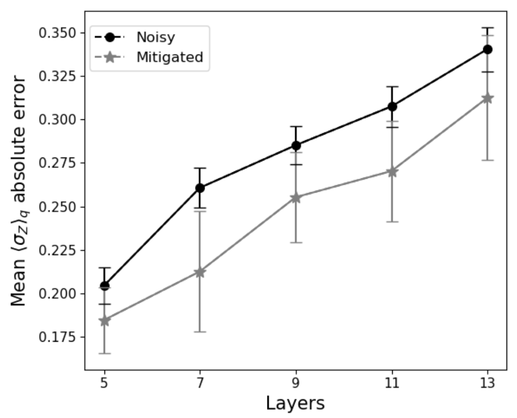
During sampling from the device, each time the target circuit is run the resulting output string is either accepted or rejected depending upon whether the acceptance threshold condition has been met in the trap circuit runs. The experiments were run across two four-qubit subsets on Aspen-9; these qubit subsets are labelled as 21, 22, 23, 24 and 32, 33, 34, 35 on the QPU specifications (see Figure 4 (a)). Each qubit was measured in the computational basis, and the local expectation values output from the individual qubits were then averaged
| (27) |
where the sum is of the expectation values in the computational basis recorded for each qubit . And so the mean absoluted error is
| (28) |
As the readout is symmeterized by the quantum one-time pad we do not need to account for the asymmetric readout errors prevalent in superconducting hardware. Each experiment consists of 750 runs of the Accreditation protocol on each of the qubit subsets, resulting in a total of 1500 runs of the Accreditation protocol per data point. Each run of the protocol consists of 15 trap circuits and the target circuit, that is 16 circuit runs in total. The order of the trap and target circuits within one protocol run is randomly assigned. Fixing the number of qubits we ran the experiment with 5, 7, 9, 11 and 13 gate layers. For each of these respectively, a trap success cutoff of greater than 6, 6, 4, 4, and 4 was used. The trap success cutoff relates to the quality factor, defining the performance threshold that has to be met for the target circuit output of a single run of Accreditation to be post-selected. For post-selection to occur, the number of trap circuit runs that do not record an error has to be greater than the designated trap success cutoff. These cutoff values were chosen heuristically depending on device performance for the particular circuit sizes. The corresponding numbers of post-selected output values were 439, 140, 238, 246 and 180. The results from this experiment can be observed in Figure 3, where the lower mean absolute errors for the post-selected sample group relative to the general sample group indicate a weaker overall noise channel in the former.
Quantum Circuit Born Machine Experiment


A quantum circuit Born machine (QCBM) is a type of generative quantum machine learning model that can be used to produce new synthetic data according to some learned distribution. It has been previously considered as representing a possible candidate for quantum machine learning to achieve a performance advantage over comparable classical generative learning models Coyle et al. 2020. The QCBM has been demonstrated on currently available quantum hardware for some small practical use-cases, for instance in learning currency pair correlations in finance Coyle et al. 2021. Generative modelling of certain discrete known distributions has previously been utilised as a convenient benchmark for QCBM performance in the presence of errors Hamilton and Pooser 2020. Here we apply the QCBM as a generative model to learn a discrete Poisson distribution, and use this to compare the closeness of the noisy to ideal distributions and also of the mitigated and ideal distributions.
To test the effect of our technique on the performance of a QCBM, a Poisson distribution was mapped onto the 16 available four-qubit computational basis states and this discrete distribution was then used as the target distribution during the training of a four-qubit, twenty-parameter QCMB on the Rigetti Aspen-11 QPU. The four-qubit subsets 34, 35, 36, 37 and 42, 43, 44, 45 were used (see Figure 4 (b)).
The circuit structure for the QCBM was the same as that shown in Figure 2 as used in the previous experiment, with alternating layers of local X rotation gates and gates. However rather than setting all of the X gate rotation parameters to like before, here the rotation parameters are trained by iterative optimization during a gradient descent algorithm which constitutes the circuit learning process. So that after training, sampling from the quantum circuit results in the output bitstrings occurring with frequencies dictated by a Poisson target distribution. The Poisson target distribution mapped onto the computational basis states is displayed Figure 5.
The QCBM was trained for 100 iterations of the COBYLA optimization algorithm Powell 1994, with the Kullback-Leibler (KL) divergence Kullback and Leibler 1951 used as the loss function during training. For each iteration of circuit training, 2000 samples were used to calculate the loss function which in this case was the KL divergence. The KL divergence is often used in the generative machine learning as a metric to represent the closeness of the noisy and ideal distributions Bang and Shim 2018. The KL divergence is defined as
| (29) |
where is the target distribution and is the noisy distribution sampled from the QCBM. The performance metrics and loss functions used in training QCBMs vary widely in the literature, with choices being made optimally according to different circumstances and applications Coyle et al. 2020. However for the purposes of demonstrating our technique it was deemed sufficient to apply the commonly used KL divergence.
Our technique was used to mitigate the time-dependent errors (here corresponding to difference in noise levels between two subsets of qubits of a quantum device) in the noisy output distribution of the trained QCBM, with the distance from the ideal distribution calculated using the KL divergence. The trained QCBM was sampled 2000 times of which 1249 were post-selected using our mitigation technique. For each run of the protocol 16 traps were used and if greater than 4 traps ran correctly the output bitstring was post-selected. The KL divergence for the unmitigated distribution was 0.624 and for the mitigated distribution was 0.531, representing a reduction in the divergence of roughly 15%. An ideal simulation of the QCBM in the absence of errors sampled 2000 times achieves a KL divergence of 0.191.

VI Discussion
In summary, we have presented an error mitigation protocol for mitigating time-dependent errors which is based on the Accreditation protocol of Ferracin et al. 2021 and post-selection. We have analyzed the sample complexity of our procedure, and shown that it provides a provable error mitigation for the important case of depolarizing noise. Finally, we ran our protocol on quantum hardware as an experimental proof of concept for the cases of a generic test circuit and a quantum circuit Born machine and obtained promising results.
A main advantage of our technique as compared to most other error mitigation techniques (see Endo et al. 2021 for a review) is that it accounts for time-dependent noise behaviours. However, a weakness in our theoretical arguments is the assumption that this time-dependent behaviour of the noise can only be one of a set of such behaviours. It would be interesting to look at ways in which we can overcome this assumption.
Furthermore, an interesting direction to pursue would be studying in detail how to integrate our error mitigation technique with other existing techniques dealing with noise which is not strongly time-dependent Endo et al. 2021.
Another important direction is adapting our protocol to work with other verification techniques, such as Fitzsimons and Kashefi 2017 which can treat more general forms of noise including so-called malicious noise coming from some adversary whose goal is to intentionally corrupt the computation.
We have run our protocol on Rigetti’s Aspen-9 and Aspen-11 quantum processors, which are based on superconducting quantum technology. It would be interesting to test the performance of our protocol on other types of quantum technologies such as photonic O’brien et al. 2009 or ion trap Kielpinski et al. 2002 technologies.
The main advantage of using the Accreditation protocol is its scalability Ferracin et al. 2021; Ferracin et al. 2019. This makes our error mitigation protocol a promising candidate to be applied on quantum circuits of sufficiently high qubit number such as to allow a convincing demonstration of quantum advantage for specific problems. We aim to explore this direction in a future work.
Acknowledgements.
We thank Marco Paini, Mark Hodson, and Theodoros Kapourniotis for fruitful discussions. We would also like to thank Mark Hodson and Alex Hill for their assistance in obtaining comprehensive Aspen-9 and Aspen-11 device specifications. R.M and E.K are grateful for support from the grant Innovate UK Commercialising Quantum Technologies (application number: 44167). J.M is supported by grant funding from the University of Edinburgh, School of Informatics. We thank the anonymous Referees as well as the Editors whose comments helped in improving this manuscript.Appendix A Appendixes
A.1 Proof of Theorem 1
Let for be independent identically distributed random variables, where for each every is chosen with uniform probability . Recall that is the expectation value (Equation (10)) corresponding to a noise behaviour with (Equation (12)), and ranges over all such behaviours. (Equation (18)) can be rewritten as
Note that for all ; denotes the expectation value of . Also, note that (Equation (19) ) for all , where denotes the variance of . We can now use Chebyshev’s inequality Saw et al. 1984 straighforwardly to obtain
| (30) |
Setting we obtain
| (31) |
Recall that we run times the Accreditation protocol, and post-select over instances where , and that there are total noise behaviours each chosen uniformly and independently (assumption ) with probability ; and out of these behaviours have . being large enough, and the distribution over noise behaviours being uniform, the law of large numbers estimates the number of runs where we obtained as
Using this and Equation (31) we obtain that
This completes the proof of Theorem 1.
A.2 Proof of Theorem 2
We will first consider the case where . Our proof idea is based on a Chernoff bound argument Chernoff 1952. Let be a random variable, , and . Our starting point is the following relation
| (32) |
Where the righmost part of Equation (32) comes from Markov’s inequality. Let (Equation (15)). From the independence assumption in section II
| (33) |
As seen previously, for is a random variable with and .
Let us now compute the moment generating function
| (34) |
It is easy to see that for , and Plugging these into Equation (34) we get
| (35) |
Note that and . Plugging these into Equation (35) and rearranging we obtain
Using the fact that for all , and setting we obtain
| (36) |
Plugging this into Equation (33) we obtain
| (37) |
plugging this into Equation (32), and then flipping this Equation (i.e considering ) with we get
| (38) |
Choosing and plugging this into Equation (38) we obtain
| (39) |
where we have relabelled (for convenience) and . In order to make our probability for the bound as large as possible, we will minimize over . Computing the derivative and setting it equal to 0, we get the following value for which maximizes
| (40) |
Note that we require , which means which implies (after replacing and solving) that . This means that and therefore (as we required in the beginning of this proof case). Replacing in Equation (39) and rearranging we obtain
| (41) |
with and Note that, because then . Now, for good accuracy, we require to be small, so , where . Note that , and also that , and from Theorem 1 we know that converges to a fixed value (i.e ) then also converges to a fixed value.
Now, . Setting and using the bound on found in Equation (31), we can choose This proves Equation (21).
Note that for the case where (), since . Also, can be made continuous by extension at since
This leads to the (trivial) bounds
and
The proof of Equations (22), (23) and (24) follows a similar path, so we will not repeat the calculations, but will remark on small differences in proving these as compared to proving Equation (21). In Equation (22) the starting point is the inequality also obtained from a Markov inequality, and we choose . In proving Equations (23) and (24) we have, , (i.e ), and . For Equation (23) the starting point is and . For Equation (24) the starting point is , and . Also in Equation (24) in order for with to be well-defined, we must have which imposes the condition (note that )
This condition is what leads to the constraint on in Theorem 2. This completes the proof of Theorem 2.
Appendix B Aspen-9 and Aspen-11 QPU Specification Information
Information on the device specifications for the Rigetti Aspen-9 and Aspen-11 QPUs is included in Figure 6 a) and b) respectively. The Aspen-9 experiments were performed on 25th September 2021, and the Aspen-11 experiments were performed on 5th February 2022. For each of the qubits used in our experiments, and for each device, we report information on qubit frequency, T1 and T2 time, gate time, gate fidelity and measurement fidelity.


References
- Arute et al. (2019) F. Arute, K. Arya, R. Babbush, D. Bacon, J. C. Bardin, R. Barends, R. Biswas, S. Boixo, F. G. Brandao, D. A. Buell, et al., Nature 574, 505 (2019).
- Zhong et al. (2020) H.-S. Zhong, H. Wang, Y.-H. Deng, M.-C. Chen, L.-C. Peng, Y.-H. Luo, J. Qin, D. Wu, X. Ding, Y. Hu, et al., Science 370, 1460 (2020).
- Aaronson and Arkhipov (2011) S. Aaronson and A. Arkhipov, in Proceedings of the forty-third annual ACM symposium on Theory of computing (2011) pp. 333–342.
- Boixo et al. (2018) S. Boixo, S. V. Isakov, V. N. Smelyanskiy, R. Babbush, N. Ding, Z. Jiang, M. J. Bremner, J. M. Martinis, and H. Neven, Nature Physics 14, 595 (2018).
- Harrow and Montanaro (2017) A. W. Harrow and A. Montanaro, Nature 549, 203 (2017).
- Preskill (2018) J. Preskill, Quantum 2, 79 (2018).
- Cerezo et al. (2020) M. Cerezo, A. Arrasmith, R. Babbush, S. C. Benjamin, S. Endo, K. Fujii, J. R. McClean, K. Mitarai, X. Yuan, L. Cincio, et al., arXiv preprint arXiv:2012.09265 (2020).
- Biamonte (2021) J. Biamonte, Physical Review A 103, L030401 (2021).
- Shor (1994) P. W. Shor, in Proceedings 35th annual symposium on foundations of computer science (Ieee, 1994) pp. 124–134.
- Grover (1997) L. K. Grover, Physical review letters 79, 325 (1997).
- Bremner et al. (2011) M. J. Bremner, R. Jozsa, and D. J. Shepherd, Proceedings of the Royal Society A: Mathematical, Physical and Engineering Sciences 467, 459 (2011).
- Bremner et al. (2016) M. J. Bremner, A. Montanaro, and D. J. Shepherd, Physical review letters 117, 080501 (2016).
- Brod and Oszmaniec (2020) D. J. Brod and M. Oszmaniec, Quantum 4, 267 (2020).
- Bremner et al. (2017) M. J. Bremner, A. Montanaro, and D. J. Shepherd, Quantum 1, 8 (2017).
- Nielsen and Chuang (2002) M. A. Nielsen and I. Chuang, “Quantum computation and quantum information,” (2002).
- Aharonov and Ben-Or (2008) D. Aharonov and M. Ben-Or, SIAM Journal on Computing (2008).
- Gottesman (1998) D. Gottesman, Physical Review A 57, 127 (1998).
- Harper and Flammia (2019) R. Harper and S. T. Flammia, Physical review letters 122, 080504 (2019).
- Nguyen et al. (2021) N. H. Nguyen, M. Li, A. M. Green, C. H. Alderete, Y. Zhu, D. Zhu, K. R. Brown, and N. M. Linke, arXiv preprint arXiv:2104.01205 (2021).
- Gertler et al. (2021) J. M. Gertler, B. Baker, J. Li, S. Shirol, J. Koch, and C. Wang, Nature 590, 243 (2021).
- Endo et al. (2018) S. Endo, S. C. Benjamin, and Y. Li, Physical Review X 8, 031027 (2018).
- Li and Benjamin (2017) Y. Li and S. C. Benjamin, Physical Review X 7, 021050 (2017).
- Temme et al. (2017) K. Temme, S. Bravyi, and J. M. Gambetta, Physical review letters 119, 180509 (2017).
- Czarnik et al. (2020) P. Czarnik, A. Arrasmith, P. J. Coles, and L. Cincio, arXiv preprint arXiv:2005.10189 (2020).
- Bennewitz et al. (2021) E. R. Bennewitz, F. Hopfmueller, B. Kulchytskyy, J. Carrasquilla, and P. Ronagh, arXiv preprint arXiv:2105.08086 (2021).
- Bonet-Monroig et al. (2018) X. Bonet-Monroig, R. Sagastizabal, M. Singh, and T. O’Brien, Physical Review A 98, 062339 (2018).
- Koczor (2020) B. Koczor, arXiv preprint arXiv:2011.05942 (2020).
- Huggins et al. (2020) W. J. Huggins, S. McArdle, T. E. O’Brien, J. Lee, N. C. Rubin, S. Boixo, K. B. Whaley, R. Babbush, and J. R. McClean, arXiv preprint arXiv:2011.07064 (2020).
- Maciejewski et al. (2020) F. B. Maciejewski, Z. Zimborás, and M. Oszmaniec, Quantum 4, 257 (2020).
- Otten and Gray (2019) M. Otten and S. K. Gray, npj Quantum Information 5, 1 (2019).
- Endo et al. (2021) S. Endo, Z. Cai, S. C. Benjamin, and X. Yuan, Journal of the Physical Society of Japan 90, 032001 (2021).
- Ferracin et al. (2019) S. Ferracin, T. Kapourniotis, and A. Datta, New Journal of Physics 21, 113038 (2019).
- Ferracin et al. (2021) S. Ferracin, S. Merkel, and A. Datta, Physical Review A 104, 042603 (2021).
- Gheorghiu et al. (2019) A. Gheorghiu, T. Kapourniotis, and E. Kashefi, Theory of computing systems 63, 715 (2019).
- Wallman and Emerson (2016) J. J. Wallman and J. Emerson, Physical Review A 94, 052325 (2016).
- (36) Note however that the work of Koczor 2020 also considered some time-dependent effects in QEM, see also Yamamoto et al. 2021.
- Geyko (2021) V. Geyko, A technical report on the progress with Rigetti platform while working on Grover’s search project, Tech. Rep. (Lawrence Livermore National Lab.(LLNL), Livermore, CA (United States), 2021).
- Brylinski and Brylinski (2002) J.-L. Brylinski and R. Brylinski, in Mathematics of quantum computation (Chapman and Hall/CRC, 2002) pp. 117–134.
- (39) See for example https://www.rigetti.com/.
- Paini et al. (2021) M. Paini, A. Kalev, D. Padilha, and B. Ruck, Quantum 5, 413 (2021).
- (41) That is, when our estimated upper bound on is .
- Takagi et al. (2021) R. Takagi, S. Endo, S. Minagawa, and M. Gu, arXiv preprint arXiv:2109.04457 (2021).
- Ville et al. (2021) J.-L. Ville, A. Morvan, A. Hashim, R. K. Naik, B. Mitchell, J.-M. Kreikebaum, K. P. O’Brien, J. J. Wallman, I. Hincks, J. Emerson, et al., arXiv preprint arXiv:2104.08785 (2021).
- Urbanek et al. (2021) M. Urbanek, B. Nachman, V. R. Pascuzzi, A. He, C. W. Bauer, and W. A. de Jong, arXiv preprint arXiv:2103.08591 (2021).
- Hong et al. (2020) S. S. Hong, A. T. Papageorge, P. Sivarajah, G. Crossman, N. Didier, A. M. Polloreno, E. A. Sete, S. W. Turkowski, M. P. da Silva, and B. R. Johnson, Physical Review A 101, 012302 (2020).
- Abrams et al. (2020) D. M. Abrams, N. Didier, B. R. Johnson, M. P. d. Silva, and C. A. Ryan, Nature Electronics 3, 744 (2020).
- Reagor et al. (2018) M. Reagor, C. B. Osborn, N. Tezak, A. Staley, G. Prawiroatmodjo, M. Scheer, N. Alidoust, E. A. Sete, N. Didier, M. P. da Silva, et al., Science advances 4, eaao3603 (2018).
- Youssef (2020) R. Youssef, Measuring and Simulating T1 and T2 for Qubits, Tech. Rep. (Fermi National Accelerator Lab.(FNAL), Batavia, IL (United States), 2020).
- (49) Https://pyquil-docs.rigetti.com/en/v2.28.0.
- Karalekas et al. (2020) P. J. Karalekas, N. A. Tezak, E. C. Peterson, C. A. Ryan, M. P. da Silva, and R. S. Smith, Quantum Science and Technology 5, 024003 (2020).
- Smith et al. (2016) R. S. Smith, M. J. Curtis, and W. J. Zeng, arXiv preprint arXiv:1608.03355 (2016).
- Smith et al. (2020) R. S. Smith, E. C. Peterson, M. G. Skilbeck, and E. J. Davis, Quantum Science and Technology 5, 044001 (2020).
- Wei et al. (2020) S. Wei, H. Li, and G. Long, Research 2020 (2020).
- Biamonte et al. (2017) J. Biamonte, P. Wittek, N. Pancotti, P. Rebentrost, N. Wiebe, and S. Lloyd, Nature 549, 195 (2017).
- Coyle et al. (2020) B. Coyle, D. Mills, and E. Kashefi, npj Quantum Information 6, 1 (2020).
- Coyle et al. (2021) B. Coyle, H. Maxwell, , J. C. J. Le, N. Kumar, M. Paini, and E. Kashefi, Quantum Science and Technology 6 (2021).
- Hamilton and Pooser (2020) K. E. Hamilton and R. C. Pooser, Quantum Machine Intelligence 2, 1 (2020).
- Powell (1994) M. J. Powell, , 51–67 (1994).
- Kullback and Leibler (1951) S. Kullback and R. Leibler, The annals of mathematical statistics 22, 79 (1951).
- Bang and Shim (2018) D. Bang and H. Shim, International conference on machine learning , 433 (2018).
- Fitzsimons and Kashefi (2017) J. F. Fitzsimons and E. Kashefi, Physical Review A 96, 012303 (2017).
- O’brien et al. (2009) J. L. O’brien, A. Furusawa, and J. Vučković, Nature Photonics 3, 687 (2009).
- Kielpinski et al. (2002) D. Kielpinski, C. Monroe, and D. J. Wineland, Nature 417, 709 (2002).
- Saw et al. (1984) J. G. Saw, M. C. Yang, and T. C. Mo, The American Statistician 38, 130 (1984).
- Chernoff (1952) H. Chernoff, The Annals of Mathematical Statistics , 493 (1952).
- Yamamoto et al. (2021) K. Yamamoto, S. Endo, H. Hakoshima, Y. Matsuzaki, and Y. Tokunaga, arXiv preprint arXiv:2112.01850 (2021).