Swapping in lattice-based cell migration models
Abstract
Cell migration is frequently modelled using on-lattice agent-based models (ABMs) that employ the excluded volume interaction. However, cells are also capable of exhibiting more complex cell-cell interactions, such as adhesion, repulsion, pulling, pushing and swapping. Although the first four of these have already been incorporated into mathematical models for cell migration, swapping has not been well studied in this context. In this paper, we develop an ABM for cell movement in which an active agent can ‘swap’ its position with another agent in its neighbourhood with a given swapping probability. We consider a two-species system for which we derive the corresponding macroscopic model and compare it with the average behaviour of the ABM. We see good agreement between the ABM and the macroscopic density. We also analyse the movement of agents at an individual level in the single-species as well as two-species scenarios to quantify the effects of swapping on an agent’s motility.
Keywords: agent-based model, lattice, swapping, cell migration, pattern formation.
I Introduction
Cell migration is an essential biological process required for the correct development of tissues and organs during embryonic development and their proper maintenance, through wound healing and tissue homeostasis, throughout life (Lauffenburger and Horwitz 1996; Plikus et al. 2021; Kulesa and Fraser 1998; Poujade et al. 2007; Deng et al. 2006). During embryonic development, neural crest cells delaminate from the dorsal most aspect of the neural tube and migrate to colonise their target tissues including the gut in the case of enteric ganglia precursors and the skin in the case of melanoblasts the precursors of melanocytes (Spritz 1994). Diseases of the neural crest are known as neurocristopathies for example failure of the enteric ganglia precursors to colonise the developing gut results in Hirschsprung’s disease (Bondurand and Southard-Smith 2016) while failure of melanoblasts to colonise the developing epidermis results in piebaldism (Mort et al. 2016). Therefore an in-depth understanding of cell migration is important for identifying the causes of neurocristopathies (Mayor and Etienne-Manneville 2016; Giniūnaitė et al. 2020; Thomas and Erickson 2008; Wang et al. 2011) as well as developing new therapeutic targets to prevent metastasis in cancers (Mayor and Etienne-Manneville 2016; Deroulers et al. 2009).
Traditionally, many biological problems have been modelled using deterministic methods. However, in cell migration, randomness can play a salient role in determining a cell’s trajectory and fate and hence deterministic theory may not be appropriate. Extensive research has gone into modelling cell movement as a stochastic process (Glazier and Graner 1993; Graner and Glazier 1992; Smith 2012; Nonaka et al. 2011; Osborne et al. 2017). In one widely used approach, cells are modelled as agents whose positions evolve probabilistically in space and time according to a predefined set of rules. These models are commonly known as agent-based models (ABMs) or individual-based models (IBMs). The agent-based modelling paradigm can be sub-divided into off-lattice and on-lattice models, both of which have wide applicability to different problems within mathematical biology. Gavagnin and Yates 2018 recently reviewed the most commonly used ABMs for cell movement.
In this paper, we only concern ourselves with on-lattice models of cell movement. In a lattice-based approach, the domain is divided into a series of compartments in which the cells reside. Cells take up space, preventing other cells from occupying the same space at the same time. For biological plausibility, it is often desirable that mathematical models of cell migration account for the single occupancy of sites. This realism is incorporated in an ABM via the volume-exclusion principle, which states that a cell attempting to move into a neighbouring site successfully moves only if the neighbouring site is not already occupied at the time of moving.
Models with volume exclusion at their core have been used to describe the collective migration of cells for a wide range of biological applications. Mort et al. 2016 used an on-lattice ABM with the exclusion principle to model the invasion of the developing epidermis by melanoblasts (the embryonic precursors of melanocytes) and investigate the basis of piebaldism in mice. Lattice-based exclusion models have also been applied to wound healing (Khain et al. 2007), migration of breast cancer cells (Simpson et al. 2010a), developmental processes on growing domains (Baker et al. 2010), cells’ responses to chemotaxis (Charteris and Khain 2014) and cells exhibiting pushing (Yates et al. 2015) and pulling (Chappelle and Yates 2019) interactions in densely crowded environments.

Biologically, although cells are excluded from the space occupied by other cells, their movement is not completely inhibited by them as typically assumed in volume-exclusion models. For example melanoblasts are able to move freely between keratinocytes in the developing epidermis (Mort et al. 2016). Experimental data suggests that cells are often able to move past each other (passing laterally, above or below) exchanging places with one another. In Figure 1 we show experimental images of two Fucci2a labelled NIH-3T3 fibroblasts exhibiting the swapping behaviour. Swapping has also been observed in blood cells such as leukocytes, erythrocytes and thrombocytes (Lan and Khismatullin 2014) and in pattern formation for maintaining sharp boundaries between different groups of cells as part of a cell sorting mechanism (Dahmann et al. 2011). These examples highlight the importance of incorporating swapping into models of cell migration. To the best of our knowledge, this has not yet been explored thoroughly from a mathematical perspective.
In this paper, we develop a mathematical model to describe and analyse cell-cell swapping in two species setting. By modifying the movement rules of the traditional volume-exclusion process, we show that swapping between agents has an effect on the migration of agents at different spatial resolutions. To investigate how swapping manifests itself in the corresponding population-level model (PLM) we derive a set of partial differential equations (PDEs) describing the macroscopic dynamics of the agents. We compare numerical solutions of the PDEs with the averaged results from the ABM and comment on the agreement or discrepancy between them. We also analyse the movement of agents at an individual level and derive expressions for the individual-level diffusion coefficient.
The remainder of this paper is structured as follows. In Section II.1, we develop a model that allows for swapping to take place between pairs of neighbouring agents. In Section II.2, we derive the macroscopic PDEs and compare the average behaviour of the ABM to that of the PDEs. In Section III, we analyse the movement of agents at an individual level and derive a relationship between the individual-level diffusion coefficient, swapping probability and background domain density. In Section IV, we give examples to illustrate the applications of swapping and finally in Section V, we conclude the paper with a summary and discussion.
II Cell migration model with swapping
We begin by developing an ABM for cell movement with swapping in Section II.1 and we use this to investigate the effect of swapping on the mobility of agents. In particular, we look at the effect of swapping on mixing of agents in a two-species system. We derive the population-level model and compare this with the average behaviour of the ABM in Section II.2. We also analyse the individual-level behaviour in both single and multispecies scenarios in Section III.
II.1 On-lattice agent-based model
We model cell migration on a two-dimensional lattice. We discretise the domain into compartments (also known as ‘sites’) such that there are compartments in the horizontal direction and compartments in the vertical direction. We assume that the compartments are square with side length . Supposing that each compartment can contain no more than one agent, can be considered a rough proxy for a cell’s diameter. A site for and can be either occupied by a type-A or a type-B agent or unoccupied. Occupancy of a site for a type-A (or type-B) agent is defined as a binary indicator, taking a value of 1 if there is a type-A (or type-B) agent at the site or 0 if the site is empty.


We initialise the lattice with species A and species B agents at densities and , respectively, such that and where is the overall domain density. We let the positions of the agents evolve in continuous time according to the Gillespie algorithm (Gillespie 1977). Let be the rate of movement of a type-A agent and let be the equivalent for a type-B agent. The rates of movement are defined such that (and equivalently ) is the probability that a type-A (or type-B) agent attempts to move during a finite time interval of duration . The agent attempts to move into one of the four sites in its Von Neumann neighbourhood with equal probability. If the chosen neighbouring site is empty, the focal agent successfully moves and its position is updated. However, if another agent already occupies the site, the move is aborted (Gavagnin and Yates 2018; Simpson et al. 2009a; Yates et al. 2015; Chappelle and Yates 2019; Simpson et al. 2009b). This blocking of the move characterises volume exclusion in our model.
Swapping works by modifying the rules of the exclusion process by allowing an exchange in the positions of a pair of neighbouring agents if the target site is already occupied. We now introduce the swapping parameter to denote the probability of a successful swap between a pair of neighbouring agents conditional on one of the agents attempting to move into the other’s position. If then there are no swaps and we arrive back at the original exclusion process. If then we can have different levels of swapping based on the value of . For example, for each scenario in which a move is attempted into an occupied target site will be a successful swap and for half of the attempted moves into occupied sites will be successful.


To implement swapping, we sample a random number from the uniform distribution over the unit interval . If , the agent at the site swaps with the agent at the target site (Figure 2-2), otherwise the move is aborted. Figure 2 shows a successful swap between two agents labelled ‘1’ and ‘2’.
In this article we present results for the two-species model only unless stated otherwise. Results for the single-species model can be found in Appendix A.
In Figure 3 we present snapshots of lattice occupancy of a 200 by 20 grid occupied with type-A (red) and type-B (green) agents. The two species move with equal rates, . We see that a non-zero swapping probability results in faster dispersion of the agents compared to the case. We also note that increasing the swapping probability from the results in faster dispersion of the agents, as expected.
In the next section, we derive the macroscopic PDEs describing the evolution of the mean lattice occupancy. By analysing the PDEs we generate further insight into the behaviours observed in Figure 3.
II.2 Continuum model
Let be the occupancy of site at time on the th repeat of the ABM such that if the site is occupied by a type-A agent and 0 otherwise. Let be the same for a type-B agent. Then the average density of type-A and type-B agents after repeats is given by,
| (1) |
In what follows we will typically drop the notation for time dependence of our species densities, i.e. and , for conciseness. By considering all the possible ways in which the site can gain or lose occupancy of either type-A or type-B agents during the time step , we can write down the corresponding occupancy master equations at time :
| (2) |
| (3) |
For illustration, we describe the terms in Equation (2). The terms in Equation (3) carry similar interpretation. A site can gain occupancy of type A in one of the following three ways:
- 1.
The site is unoccupied and a type-A agent moves in from a neighbouring site (line 1 in Equation (2)).
- 2.
The site is occupied by a type-B agent, which initiates and completes a swap with a type-A agent at a neighbouring site (line 3 in Equation (2)).
- 3.
The site is occupied by a type-B agent and a type-A agent at a neighbouring site initiates a swap to exchange positions with the type-B agent in the site (also line 3 in Equation (2)).
In all three cases, a type-A agent moves into the site . Similarly, there are three ways for a type-A agent to move out of the site leading to a loss in the corresponding occupancy:
- 1.
The site is occupied by a type-A agent which jumps out to an unoccupied neighbouring site, leaving the site empty (line 2 in Equation (2)).
- 2.
The site is occupied by a type-A agent which initiates a swap with a type-B agent in its neighbourhood.
- 3.
The site is occupied by a type-A agent and a type-B agent in the neighbouring site initiates a swap to exchange positions with the agent in site (line 4 in Equation (2)).
In all three cases, a type-A agent moves out of the site .
To obtain the continuum model, we Taylor expand the appropriate terms on the RHS of Equations (2) and (3) around the site keeping terms of up to second order. By letting and such that is held constant, we arrive at the coupled PDEs,
| (4) | ||||
| (5) |
where,
| (6) |
| (7) |
Here,
are the macroscopic diffusion coefficients corresponding to species A and B, respectively. Setting in equations (4) and (5) leads to,
| (8) | ||||
| (9) |
which are the macroscopic equations for the two-species volume-exclusion process (Simpson et al. 2009b).


In Figure 4, we compare the column-averaged density of the ABM given by,
to the numerical solution of the one-dimensional analogue of Equations (4) and (5) with reflective boundary conditions by averaging the PDEs over the direction11 1 Note that in Figure 4 in the fully occupied domain the agreement is trivially perfect since volume exclusion prohibits departure from the initial condition.. In the case (Figure 4, first column), the PDE solutions and the ABM do not agree well as evidenced by the disparity between the two profiles. This discrepancy can also be seen in Simpson et al. 2009b where the authors devise an ABM for multi-species exclusion processes ( case in our model) and compare their ABM with the corresponding continuum model. We remark that one reason for the discrepancy is that in crowded environments where the movement of agents is frequently inhibited by other agents, lattice occupancies cannot be considered independent of each other and spatial correlation are not dissipated efficiently (Simpson et al. 2013; Markham et al. 2013a; Markham et al. 2013b). Independence of lattice sites is a key assumption that is typically made when deriving the continuum models such as the one above (Simpson et al. 2007; Simpson et al. 2009b; Simpson et al. 2010a; Simpson et al. 2009a; Gavagnin and Yates 2018; Chappelle and Yates 2019; Yates et al. 2015).
For non-zero swapping probabilities, the agreement is significantly improved between the deterministic and stochastic model (Figure 4, second and third columns). Swapping helps to break down the spatial correlations improving the agreement between the PLM and the ABM. We also see that in the zero swapping case, crowding of the green agents behind the red agents leads to profiles for which the maximum density at non-zero time (shown and in Figure 4) is higher than the initial maximum density (). The reason for this is that for a multispecies migration process with cross-diffusion terms there is no maximum principle for the individual species (Rahman et al. 2016; Jüngel 2015; Simpson et al. 2009b). We note that the enhanced diffusion which swapping engenders eliminates this effect. However, this does not necessarily mean that a maximum principle now holds for the systems under consideration. Investigating this further is beyond the scope of this article.
III Individual-level analysis
In this section, we analyse the movement of agents at the individual level in the single-species and two-species case to assess how swapping affects the movement of agents.
III.1 Single-species individual-level analysis
The single-species swapping discrete and continuum models are given in Appendix A. Here, we present the individual-level analysis for the single-species model. Our aim is to quantify the movement of individually tagged agents by their individual-level diffusion coefficient. For the analysis that we present next, we neglect any long range temporal correlations in the agents’ movement. We first derive the individual-level time-uncorrelated diffusion coefficient analytically and then we compare it with its ABM approximation.
Let denote the probability that a focal agent is at position at time . Defining as an infinitesimally small change in time, we can write down the probability of the agent being at position at time as,
| (10) |
A lattice site is occupied with probability and empty with probability . The first four terms in Equation (10) are obtained by considering an agent at each of the four lattice sites in the neighbourhood the site that has attempted to move into site with probability . If the site is vacant, the agent jumps from the neighbouring site to site . Otherwise, the agents at the neighbouring site and site swap their positions with probability . The 2 in corresponds to the two ways in which the position of the agent at site can change due to a swap: either the agent at site initiates and successfully completes the swap with the agent at the neighbouring site or the agent at the neighbouring site initiates and successfully swaps with the agent at site . The last term in Equation (10) gives the probability that the agent already occupying position does not attempt to move during the time interval with probability and the probability that the agent attempts to swap with an agent at an occupied neighbouring site but fails to complete the swap with probability and lastly the probability that a neighbouring agent successfully swaps with the agent at site with probability .
By rearranging, dividing both sides of Equation (10) by and taking the limit as leads to the system of ODEs given by,
| (11) |
which describe the time evolution of the probability of finding an agent at position at time . From Equation (11) it can be shown that the expected net displacement of an agent is zero. This gives us no information about the statistical fluctuations in the movement of an agent and therefore we use the variance to quantify the net displacement (Codling et al. 2008; Simpson et al. 2009a). The equations describing the time-evolution of the variances and are given by,
| (12) |
and,
| (13) |
| (14) |
The time-uncorrelated individual-level diffusion coefficient can be retrieved as,
| (15) |
As briefly discussed above, the master equation neglects temporal correlations in an agent’s position. Consequently, the diffusion coefficient derived from the master equation will necessarily be inaccurate and fail to represent the true dynamics of the agents in the system. As a result, we refer to the expression given in Equation (15) as the time-uncorrelated individual-level diffusion coefficient.
To approximate the using the ABM, we initialise a by lattice and randomly seed it with agents at different background densities , where corresponds to one agent with no agents in the background to interact with and corresponds to a fully populated lattice. We let the positions of the agents evolve according to the single-species version of the ABM described in Section II.1 using the movement rate for a range of swapping probabilities . The positions of agents whose initial position is in the region defined by the central square are recorded over a regular time grid to create a track where is the recording step and is the track length. Each track traces the path of an agent over time. We impose periodic boundary conditions on the domain. The simulation ends at or when a tracked agent hits a boundary, whichever happens first.
We analyse individual movement of agents using the sum of squared displacement (SSD) (Simpson et al. 2009a; Simpson et al. 2007),
| (16) |
and,
| (17) |
By only taking the difference between successive positions, the SSD neglects temporal correlations in an agent’s position which is consistent with our master equation in Equation (10). For each value of and we average the SSD over an ensemble of tracks and fit a linear model of the form and in each orthogonal direction and , respectively. The ABM approximation of the time-uncorrelated individual-level diffusion coefficient can be extracted from the gradient of these linear equations,
| (18) |
where is the dimension dimension of the lattice. We put a ‘hat’ symbol over to differentiate it from the exact time-uncorrelated diffusion coefficient in Equation (15).


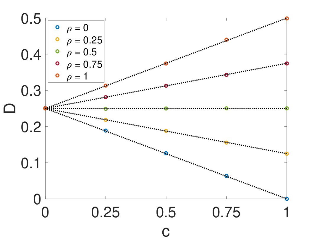
In Figure 5, we compare the ABM approximation (shown in 5) with the derived expression (shown in 5) as a pair of heat maps for the range of values of and defined earlier. We also show a line plot that nicely depicts the linear relationship between and for different value of (shown in 5). We can see that there is excellent agreement between the analytical expression and the simulated results. We note that in the case of zero background density () is always 0.25 regardless of the swapping probability since for a single agent with no other agents to interact with, the movement of the agent can neither be inhibited by volume exclusion nor enhanced by swapping. We also note that for swapping probability , the value of is always 0.25 irrespective of the density since half the number of times a focal agent attempts to move into an occupied site the moves will be rejected. If this were the only impact of swapping, we would expect of the focal agent to be reduced. However, just as often as a focal agent attempts to move into an occupied neighbour’s position, an agent occupying a neighbouring site tries to move into the focal agent’s position – achieving this successfully with probability . Assuming a well-mixed scenario, this exactly compensates for the number of aborted moves the focal agent makes, meaning movement is as if the focal agent were on an unoccupied domain irrespective of density. For and we note that (i.e. twice as large compared to an agent moving on a domain with zero background density) as every attempted move by the focal agent is executed successfully and the focal agent is also moved equally often by neighbouring agents swapping into its position.
III.2 Two-species individual-level analysis
In this section, we perform the individual-level analysis for a two-species system as set out for the single-species case in Section III.1.
Let be the probability that a focal agent of type-A occupies the position and let be the equivalent for a type-B focal agent. Recalling as a small change in time we can write down the master equations for species A and B at time ,
| (19) | ||||
| (20) |
The individual-level time-uncorrelated diffusion coefficients and for the species A and B, respectively, are given by,
| (21) | ||||
| (22) |
In order to investigate the effect of swapping on a two-species system and to verify our theoretical results, we simulate the two-species model, track a set of tagged agents and analyse their movement using the SSD as done in Section III.1.


In Figure 6 we show the time-uncorrelated diffusion coefficient of species A and species B plotted against background density for different values of swapping probability , for the specific case in which and . In this figure, both species are present in equal proportions on the domain. We see good agreement between the ABM approximations and the theoretical values. We also see that, as expected and as noted in the single-species system, swapping speeds up the movement of the agents in the multi-species setting compared to the pure volume-excluded scenario (). Furthermore, since species B has a higher movement rate than species A, species B diffuses faster than species A, apart from the and trivial case in which and are both 0 since the agents have nowhere to go.
In Figure 7 we present a similar comparison as in Figure 6 but this time the two species are not present in equal proportions. In this particular case, we consider a scenario in which type-A agents make up 25% of the total population and type-B agents 75%. Again, we see good agreement between the ABM and theoretical values and that swapping speeds up the movement of agents.
Comparing Figure 6 to Figure 7 we see that for the case and in Figure 6 are equal to their respective values in Figure 7 and hence unaffected by changes in the densities and . Analytically, this can be observed by setting in Equations (21) and (22). In this case, and depend on the overall background density and not the species proportions. For , in the instance where both species show faster movement in Figure 7 than in Figure 6. Again, this can be checked by referring to the expressions for and . Changing the proportions of the species (while keeping , and constant) the term is sensitive to changes in the proportions in both and . When and we increase the proportion of the faster moving species, , this results in more swapping events which enhance the movement of both species. On the other hand, if we were to increase the proportion of species A (while simultaneously decreasing the proportion of species B to keep constant) we would observe reduced movement for both species since an increase in the proportion of the slower moving species (and a decrease in the proportion of faster moving species) would result in fewer swaps.
IV Illustrative examples
In this section, we show examples of the situations in which swapping has important applications. In Section IV.1, we build the swapping mechanism into a cell migration model with proliferation and in Section IV.2, we show how the swapping mechanism in conjunction with cell-cell adhesion can facilitate spontaneous pattern formation in densely crowded environments.
IV.1 Swapping model with cell proliferation
We look at the role of swapping in cell migration with proliferation. For this example, we concern ourselves with the two-species cell migration model. The movement kinetics of the agents are the same as the swapping model described in Section II.1 but in addition to migrating, agents can attempt to proliferate, placing a daughter at a randomly chosen neighbouring site if the site is empty, otherwise the division event is aborted. The proliferation rates per unit time for the two species A and B are denoted by and , respectively.
We initialise the domain with sites in the horizontal direction and sites in the vertical direction. We fill all the sites in the range with agents of type A and all the remaining sites with type-B agents at a density of 0.5. The movement rates of agents are set to and the proliferation rates as and , i.e. only the agents of type A divide and the number of type-B agents are held constant. We let the system evolve according to the specified ABM.
In Figure 8 we provide snapshots of the evolving lattice occupancy for (columns 1, 2 and 3, respectively) at (rows 1, 2 and 3, respectively). We see, at the same time points, that cells are unsurprisingly more well-mixed in the case of non-zero swapping (second and third columns in Figure 8) compared to the zero-swapping situation (first column in Figure 8). We also see faster colonisation of the domain overall in the non-zero swapping cases than without swapping. This is because swapping allows the proliferating red agents to disperse more quickly into less dense regions, which in turn increases the probability of a successful division events for these agents. Without swapping, it takes longer for proliferative red agents to find the space to proliferate into. This trend of decreasing colonisation time with increasing swapping probability is reinforced in Figure 9 where we see that the time to reach the domain’s carrying capacity is a decreasing function of the swapping probability, .


The mean-field PDEs describing the approximate population-level dynamics of the agent are given by,
| (23) | ||||
| (24) |
where and are as defined previously. Notice that proliferation of type-A agents gives rise to an additive source term in Equation (23). The derivation of this source is standard and can be found in Plank and Simpson 2012; Simpson et al. 2010b, for example.
In Figure 10 we compare the average column density of the ABM with the numerical solution of the one-dimensional analogue of the mean-field PDEs obtained by averaging over the direction with . We chose this value for the proliferation rate as we wanted to keep the ratio (Fadai et al. 2019; Simpson et al. 2010b). There are two reasons for this: firstly, a modelling choice to prevent agents clustering into proliferation-induced patches and secondly, it is biological realism that given the parameters of the model we could expect real biological cells will attempt proliferation events less frequently than movement events. We see good agreement between the two profiles for non-zero swapping probability. However, when the swapping probability is set to 0, we see discrepancies arising that are amplified as time increases. Recall that the disparity between the PDE and ABM profiles can be also observed in Figure 3 due to spatial correlations that are not accounted for by the mean-field PDEs. The addition of proliferation into the model increases the spatial correlations between site occupancies, leading to greater disparity. One way to partially rectify this problem is by modelling the higher order moments in the PDE description (Markham et al. 2013a; Markham et al. 2013b; Simpson et al. 2013) however for the purposes of this work, we simply note that allowing swapping breaks up the correlations more effectively than in its absence leading to better agreement between the ABM and the population-level densities.
IV.2 Swapping model with cell-cell adhesion
Another interesting application of swapping is the formation of patterns in densely crowded environments. In this section, we use a cell-cell adhesion model with swapping to investigate how biologically plausible patterns can form starting from a randomly seeded domain. Our model is based on the similar cell-cell adhesion model studied previously by (Simpson et al. 2010a; Charteris and Khain 2014; Khain et al. 2007) who consider adhesion between identical agents. Here, we extend the model to incorporate two types of agents with swapping to facilitate the movement events.
For the purpose of this paper, we assume adhesion between two species, A and B, on a fully populated domain. For a simple exclusion-based ABM the agents on the fully populated domain would not successfully move at all. This is since the exclusion principle forbids cells from occupying the already occupied lattice sites. In our model, the movement of the agents and the formation of patterns will be facilitated by the swapping mechanism. In an on-lattice adhesion model, agents can adhere to other agents in their neighbourhood, making them less likely to successfully complete the movement event. As well as the number of agents in the neighbourhood, the strength of adhesion determines how likely an agent is to successfully move. In a simple model with species A and B, characterises the strength of adhesion between two type-A agents and the strength of adhesion between two type-B agents.
We assume cell movement in a densely crowded domain where the underlying lattice is fully populated with type-A and B agents, their positions chosen uniformly at random. When an agent is chosen to move into an occupied neighbouring site, we check the feasibility of swapping by sampling a random number from the standard uniform distribution and comparing it with the swapping probability, . A swapping move breaks existing interactions between the two swapping agents and their neighbours and makes new connections following a successful swap. Since the movement of the focal agent and the target agent depends on their respective neighbours, the success of a swapping move depends on whether the respective neighbouring sites are occupied by type-A or type-B agents. Suppose the focal agent is at site and let be the set containing the positions its neighbouring sites on the two-dimensional lattice. If the focal agent is a type-A agent then the probability of it breaking existing connections with its neighbours is given by,
| (25) |
However, if the focal agent is a type-B agent then,
| (26) |
Here, are binary taking a value of unity if the site with position is occupied by a type-A agent or 0 otherwise. Therefore, is the sum of occupancies of the sites in that are occupied by type-A agents. Likewise, is the sum of occupancies of the sites in that are occupied by type-B agents. Similarly, for a type-A agent occupying the target site the probability that it breaks existing connections with its neighbours is given by,
| (27) |
However, if the agent occupying the target site is a type-B agent then,
| (28) |
Here, the set contains the positions of sites in the neighbourhood of the target site, . Therefore, is the sum of occupancies of all the sites in that are occupied by a type-A agent and denotes the sum of occupancies of all the sites in that are occupied by a type-B agent.
The probability of a successful swap given a movement event has been attempted is therefore a product of the swapping probability, the probability of the focal agent at site breaking links with its neighbours in order to move out and the probability of the agent at the target site breaking links with its neighbours in order to move in, i.e.,
| (29) |
Here we are considering that the link between the two swapping agents has to be broken in order for the swap to take place. As an example, consider the case in which the focal agent at site attempts to jump into the neighbouring site (Figure 11). The agent occupying the focal site is a type-A agent, shown in red and labelled as 1 and the target site is occupied by a type-B agent, shown in green and labelled as 2. Since the focal agent is red, it is adhesive to other red agents in its Von Neumann neighbourhood. There is only one site (with position ) neighbouring agent 1 that is occupied by a red agent and therefore, . Since agent 2 (target site) is a green agent, it is adhesive to the other green agents in its Von Neumann neighbourhood. There is only one green agent in the neighbourhood (position ) and hence, . For an arbitrary , and , the probability of swap in this situation given a neighbouring site to move into has already been chosen can be written as .


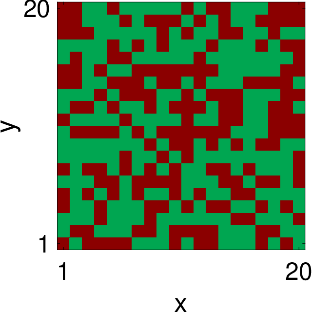


In Figure 12, we present some results that demonstrate the importance and impact of swapping in a model of adhesion-mediated pattern formation. For this, we consider a square lattice with sites in both the horizontal and vertical direction. As before, one compartment can accommodate no more than a single agent at a time. We impose periodic boundary conditions. We seed the lattice with type-A and type-B agents at a density of 0.5 each, where the initial positions of the agents on the lattice are assigned uniformly at random (Figure 12). We let positions of the agents evolve according to the kinetics described above using the movement rate and .
Snapshots of the evolving lattice occupancy at for two different sets of and values are shown in Figure 12 and 12. We can see self-organisation of agents into clusters of like type agents. The characteristic size of the aggregates is sensitive to the magnitude of the adhesion strengths. The clusters are bigger where self-adhesion within one species is stronger than within the other ( and ) whereas we see more labyrinthine patterns when both the adhesion strengths are very strong and equal (). It is evident from these figures that in densely crowded domains, swapping plays a vital role in allowing agents to organise themselves to form patterns. Without swapping, no agent movement and hence no pattern formation would be possible.
V Discussion and conclusion
Cell movement is often modelled as a volume-exclusion process. However, in reality cell movement is not completely inhibited volume exclusion. In this paper, motivated by real-life examples, we developed an ABM that allows a pair of neighbouring agents to swap positions with each other. Our model maintains the important carrying capacity component of volume-exclusion models but allows the flexibility of movement observed even amongst some densely packed configurations. We considered a two-species system and allowed it to evolve according to the dynamics of our model. We found that swapping enhances the movement of agents by allowing agents to mix more compared to the pure volume-exclusion model. Comparing the ABM to the population-level model we found excellent agreement between the two as long as the swapping probability was sufficiently large.
To understand how swapping affects agent movement at an individual level, we analysed simulated agent tracks to determine the time-uncorrelated individual-level diffusion coefficient. We found that swapping enhanced the movement of agents in all cases compared to the volume-exclusion model. Using the probability master equation, we were able to analytically derive an expression for the diffusion coefficient that confirms the relationship obtained via the simulated tracks.
In Section IV, we demonstrated the importance of swapping via a couple of examples. In the first application, we considered a cell migration model with proliferation. We found that swapping accelerates the proliferation process by allowing the agents to disperse more and breaking spatial correlations. We found that the time to reach the domain’s carrying capacity varies inversely with the swapping probability. Deriving the PLM and comparing it to the average density of the ABM, we showed that there is a good agreement between the two profiles for sufficiently large swapping probability. For the case, we note discrepancies that are caused by the build up of spatial correlations between sites.
For the second example, by incorporating swapping into a cell-cell adhesion model, we showed that agents can spontaneously rearrange themselves into clusters to form patterns even on densely populated domains. We stress that without swapping these patterns would not be realised. Biological patterns involving cell-cell adhesion have been observed amply in experimental work. Honda et al. 1986 reported chequered patterns in Japanese quail oviduct epithelium which were later modelled mathematically by Glazier and Graner 1993 using a cellular Potts model. Armstrong 1971 observed sorting of neural and pigmented retinal epithelial cells in chick embryo where neural cells completely engulfed the pigmented cells from an initially disordered arrangement. Engulfment was modelled mathematically using a cellular Potts model (Glazier and Graner 1993; Graner and Glazier 1992) and by Armstrong et al. 2006 using a continuous approach.
Models incorporating swapping may prove useful when analysing multi-species systems in which cells need to migrate in a crowded epithelium or tissue parenchyma. These systems are often interrogated experimentally using the generation of chimaeras or mosaics, analysing the resulting patterns generated by cell mixing (Chang et al. 2011; Landini and Iannaccone 2000; Petit and Nicolas 2009; Mort et al. 2011; Mort et al. 2009). For example the generation of corneal epithelial stripes in X-inactivation mosaic female mice hemizygous for an X-linked copy of the LacZ gene, expressing the enzyme -galactosidase (Tan et al. 1993). Here, a mixture of -gal positive and -gal negative limbal epithelial cells are specicifed as limbal stem cells whose progeny then migrate centripetally to generate -gal positive and -gal negative corneal epithelial stripes (Collinson et al. 2002). Experiments suggest that the degree of mixing of the limbal progenitors will generate stripes of different width composed of multiple clones of the same colour (Tan et al. 1993). Swapping would be useful in understanding how cell mixing at the limbus impacts the final stripe pattern generated.
In conclusion, motivating our study by real-life examples, we have developed a cell migration model that incorporates swapping as a viable movement process. As well as adding biological realism, our model has the added benefit of better agreement between the corresponding continuum description and the ABM compared to the classical volume-exclusion process. We also saw that the ABM with swapping and cell-cell adhesion, when applied to cells in densely crowded environments, leads to pattern formation. We once again stress that the patterns would be unattainable under the traditional volume-exclusion model. The results in this paper hint that swapping is an important and overlooked mechanism in the context of modelling real biological scenarios and merits further explorations in conjunction with experimental data.
Acknowledgements
Shahzeb Raja Noureen is supported by a scholarship from the EPSRC Centre for Doctoral Training in Statistical Applied Mathematics at Bath (SAMBa), under the project EP/S022945/1. This research made use of the Balena High Performance Computing (HPC) Service at the University of Bath. The images in Figure 1 were taken by Dr. Matthew Ford (Centre for Research in Reproduction and Development, McGill, Canada). Richard Mort was supported by North West Cancer Research (NWCR Grant CR1132) and the NC3Rs (NC3Rs grant NC/T002328/1). We would like to thank the members of Christian A. Yates’ mathematical biology journal club for constructive and helpful comments on a preprint of this paper. Finally, we would like to thank Fraser Waters for his help in managing some of the code related to this project.
Appendices
Appendix A Single-species PDE vs. ABM results
Below we summarise the single-species swapping model and present results comparing the discrete and continuum models.
The single-speices model is a simplified version of the two-species model in the sense that there is only species on the domain of interest at density and hence only a single movement rate. We summarise the the model here.
We let be the rate of movement of an agent such that is the probability that the agent attempts to move during a finite time interval of duration . The agent attempts to move into one of its four neighbouring sites with equal probability. If the chosen neighbouring site is empty, the focal agent successfully moves and its position is updated. If another agent already occupies the site, the agent at site attempts to swap positions with the neighbouring agent with probability . If the swap is successful, the two agents exchange positions with each other. Otherwise, the move is aborted.


In Figure 13 we present snapshots of the lattice occupancy for the single-species model at and for swapping probabilities with with reflective boundary conditions. We see that swapping seems to have no effect on the dispersion of the agents at a macroscopic scale as the density profiles are indistinguishable regardless of the swapping probability. If two agents are identical to each other and unlabelled then exchanging positions by swapping is equivalent to an aborted movement attempt in the volume-exclusion process and produces no change in the state of the system.
In the next section, we derive the macroscopic PDE describing the evolution of the mean lattice occupancy in the single-species model.
A.1 Single-species continuum model
Let be the occupancy of site on the th repeat at time , where if the site is occupied and otherwise. The average occupancy of site at time after runs is then given by,
| (30) |
Let for conciseness. By considering the possible movement events of the agent at the site during the small time step (Yates et al. 2015; Chappelle and Yates 2019), we can write down the master equation for the occupancy of the site at time ,
| (31) |
The site can gain occupancy if it is unoccupied at time and the agent from a neighbouring site moves in (first line on the RHS of Equation (31)). Similarly, the site can lose occupancy if the site is occupied at time and the residing agent jumps out to a neighbouring compartment, leaving the site empty (second line in Equation (31)). Movement of agents due to a successful swapping event is captured by the lines 3-6 in Equation (31). However, since the agents are assumed to be identical and unlabelled lines 3-6 cancel each other out, eliminating the effect of swapping. Consequently, we are left with lines 1 and 2 only. Taylor expanding these remaining terms around the site up to second-order and taking the limit as gives the diffusion equation, as expected:
| (32) |
Here,
is the diffusion coefficient given that is held constant in the diffusive limit. Equation (32) describes the evolution of the lattice occupancy over time. It is well-known that for the simple exclusion process, the occupancy is described by the diffusion equation (Simpson et al. 2009b; Gavagnin and Yates 2018). It makes sense therefore that in Figure 13 swapping made no difference to the overall occupancy of the lattice. In Figure 14 we compare the average column density of the ABM which is given by,
to the solution of the one-dimensional analogue of Equation (32) with reflective boundary conditions by averaging the PDEs over the direction.
As expected, we see an excellent agreement between the two density profiles. We also see that there is perfect agreement even in the zero-swapping case which we did not see in the two-species example in Section II.2. This is because in a single-species system there is no way of distinguishing between a successful swapping of the position of a pair of neighbouring agents and an aborted movement event due to the volume-exclusion principle. This leads to identical profiles for different regardless of its magnitude.
In contrast to the two-species case, here there is perfect agreement between the ABM and the PDE profiles since in the single-species case the agents are indistinguishable from each other. In the two-species scenario, because the agents are competing for space, in the no-swapping situation one species affects the occupancy of the other, leading to spatial correlation and discrepancy between the ABM and PDE descriptions. Swapping serves to break up the correlation and improve agreement between the discrete and continuum models.


Appendix B Two-species individual-level diffusion coefficients
Let be the probability that a type-A agent occupies the site and let be the equivalent for species B. We can write down the master equation for species A and species B at time where is a small change in time,
| (33) | ||||
| (34) | ||||
We explain the meaning of the terms in the discrete-time master Equation (33). Equation (34) can be interpreted similarly. The equations describe the evolution of the probability that a focal agent of type A is occupying site by considering possible movement events of the focal agent at site and agents at neighbouring sites. Firstly, the terms which correspond movements that increase the probability that the focal agent sits at position are as follows:
- 1.
The focal type-A agent residing at a neighbouring site moves into the empty site (line 1, term 1).
- 2.
The focal type-A agent at a neighbouring site initiates and successfully completes a swap with a type-A agent at site or, alternatively a type-A agent at site initiates the swap and exchanges position with the focal type-A agent at the neighbouring site (hence the multiplier 2 for the two equally likely probabilities) (term 2 on line 1 through line 2 up to first closing square bracket).
- 3.
The focal type-A agent at a neighbouring site initiates and successfully swaps with a type-B agent at site (term 2 on line 2).
- 4.
A type-B agent at site initiates and successfully swaps positions with the focal type-A agent at a neighbouring site (term 1 on line 3).
Secondly the terms which correspond to the site already being occupied and no event occurring to change that state correspond to the terms inside the pair of square brackets which spans lines 3 and 4. Recalling that the probability of nothing happening in the time interval is unity minus the probability that something happens, the terms in square brackets can be described as follows:
- 1.
The unit corresponds to the probability that the focal agent occupied site at time .
- 2.
The second term correspond to the focal type-A agent at site moving to an unoccupied neighbouring site.
- 3.
The third term corresponds to the probability that the focal agent of type A at site initiates and successfully swaps with a type-A agent at a neighbouring site and the probability that a type-A agent at a neighbouring site initiates and successfully swaps with the focal agent of type A at site (hence the factor of 2 for these equally probably events).
- 4.
The fourth term corresponds to the probability that the focal type-A agent at position initiates and successfully swaps with a neighbouring agent of type B.
- 5.
Finally, the fifth term in the square brackets corresponds to a type-B agent at a neighbouring site successfully swapping positions with the type-A focal agent occupying site .
Subtracting from both side and dividing by and taking the limit as gives,
| (35) |
| (36) |
After using the definitions in Equation (12) and (13), and suitably transforming the indices and , after simplifying it can be shown that the equations describing the evolution of the second moment of the position and of species A and B are given by,
| (37) |
| (38) |
Given that ,
Thus,
| (39) | ||||
| (40) |
are the individual-level time-uncorrelated diffusion coefficients of species A and B, respectively.
References
- Lauffenburger and Horwitz (1996) D. A. Lauffenburger and A. F. Horwitz, Cell 84, 359 (1996).
- Plikus et al. (2021) M. V. Plikus, X. Wang, S. Sinha, E. Forte, S. M. Thompson, E. L. Herzog, R. R. Driskell, N. Rosenthal, J. Biernaskie, and V. Horsley, Cell 184, 3852 (2021).
- Kulesa and Fraser (1998) P. M. Kulesa and S. E. Fraser, Developmental Biology 204, 327 (1998).
- Poujade et al. (2007) M. Poujade, E. Grasland-Mongrain, A. Hertzog, J. Jouanneau, P. Chavrier, B. Ladoux, A. Buguin, and P. Silberzan, Proc. Natl. Acad. Sci. 104, 15988 (2007).
- Deng et al. (2006) M. Deng, W.-L. Chen, A. Takatori, Z. Peng, L. Zhang, M. Mongan, R. Parthasarathy, M. Sartor, M. Miller, J. Yang, B. Su, W. W.-Y. Kao, and Y. Xia, Mol. Biol. Cell 17, 3446 (2006).
- Spritz (1994) R. A. Spritz, J. Invest. Dermatol. 103, S137 (1994).
- Bondurand and Southard-Smith (2016) N. Bondurand and E. M. Southard-Smith, Dev. Biol. Enteric Nervous System, 417, 139 (2016).
- Mort et al. (2016) R. L. Mort, R. J. Ross, K. J. Hainey, O. J. Harrison, M. A. Keighren, G. Landini, R. E. Baker, K. J. Painter, I. J. Jackson, and C. A. Yates, Nat Commun 7, 1 (2016).
- Mayor and Etienne-Manneville (2016) R. Mayor and S. Etienne-Manneville, Nat. Rev. Mol. Cell Biol. 17, 97 (2016).
- Giniūnaitė et al. (2020) R. Giniūnaitė, R. E. Baker, P. M. Kulesa, and P. K. Maini, J. Math. Biol. 80, 481 (2020).
- Thomas and Erickson (2008) A. J. Thomas and C. A. Erickson, Pigment Cell Melanoma Res. 21, 598 (2008).
- Wang et al. (2011) X. Wang, A. K. Chan, M. H. Sham, A. J. Burns, and W. Y. Chan, Gastroenterology 141, 992 (2011).
- Deroulers et al. (2009) C. Deroulers, M. Aubert, M. Badoual, and B. Grammaticos, Phys. Rev. E 79, 031917 (2009).
- Glazier and Graner (1993) J. Glazier and F. Graner, Phys. Rev. E 47, 2128 (1993).
- Graner and Glazier (1992) F. Graner and J. A. Glazier, Phys. Rev. Lett. 69, 2013 (1992).
- Smith (2012) A. Smith, Vertex Model Approaches to Epithelial Tissues in Developmental Systems, Ph.D. thesis, Oxford University, UK (2012).
- Nonaka et al. (2011) S. Nonaka, H. Naoki, and S. Ishii, Neural Netw. 24, 979 (2011).
- Osborne et al. (2017) J. M. Osborne, A. G. Fletcher, J. M. Pitt-Francis, P. K. Maini, and D. J. Gavaghan, PLoS Comput. Biol. 13, e1005387 (2017).
- Gavagnin and Yates (2018) E. Gavagnin and C. A. Yates, in Handbook of Statistics, Vol. 39 (Elsevier, 2018) pp. 37–91.
- Khain et al. (2007) E. Khain, L. M. Sander, and C. M. Schneider-Mizell, J. Stat. Phys. 128, 209 (2007).
- Simpson et al. (2010a) M. J. Simpson, C. Towne, D. S. McElwain, and Z. Upton, Phys. Rev. E 82, 041901 (2010a).
- Baker et al. (2010) R. E. Baker, C. A. Yates, and R. Erban, Bull. Math. Biol. 72, 719 (2010).
- Charteris and Khain (2014) N. Charteris and E. Khain, New J. Phys. 16, 025002 (2014).
- Yates et al. (2015) C. A. Yates, A. Parker, and R. E. Baker, Phys. Rev. E 91, 052711 (2015).
- Chappelle and Yates (2019) G. Chappelle and C. A. Yates, Phys. Rev. E 99, 062413 (2019).
- Mort et al. (2014) R. L. Mort, M. J. Ford, A. Sakaue-Sawano, N. O. Lindstrom, A. Casadio, A. T. Douglas, M. A. Keighren, P. Hohenstein, A. Miyawaki, and I. J. Jackson, Cell Cycle 13, 2681 (2014).
- Lan and Khismatullin (2014) H. Lan and D. B. Khismatullin, Phys. Rev. E 90, 012705 (2014).
- Dahmann et al. (2011) C. Dahmann, A. C. Oates, and M. Brand, Nat. Rev. Genet. 12, 43 (2011).
- Gillespie (1977) D. T. Gillespie, J. Phys. Chem. 81, 2340 (1977).
- Simpson et al. (2009a) M. J. Simpson, B. D. Hughes, and K. A. Landman, Australas. J. Eng. Educ. 15, 59 (2009a).
- Simpson et al. (2009b) M. J. Simpson, K. A. Landman, and B. D. Hughes, Phys. A 388, 399 (2009b).
- (32) Note that in Figure 4 in the fully occupied domain the agreement is trivially perfect since volume exclusion prohibits departure from the initial condition.
- Simpson et al. (2013) M. J. Simpson, B. J. Binder, P. Haridas, B. K. Wood, K. K. Treloar, D. S. McElwain, and R. E. Baker, Bull. Math. Biol. 75, 871 (2013).
- Markham et al. (2013a) D. C. Markham, M. J. Simpson, P. K. Maini, E. A. Gaffney, and R. E. Baker, Phys. Rev. E 88, 052713 (2013a).
- Markham et al. (2013b) D. C. Markham, M. J. Simpson, and R. E. Baker, Phys. Rev. E 87, 062702 (2013b).
- Simpson et al. (2007) M. J. Simpson, A. Merrifield, K. A. Landman, and B. D. Hughes, Phys. Rev. E 76, 021918 (2007).
- Rahman et al. (2016) K. Rahman, S. Sonner, and H. Eberl (2016).
- Jüngel (2015) A. Jüngel, Nonlinearity 28, 1963 (2015).
- Codling et al. (2008) E. A. Codling, M. J. Plank, and S. Benhamou, J R Soc Interface 5, 813 (2008).
- Plank and Simpson (2012) M. J. Plank and M. J. Simpson, J R Soc Interface 9, 2983 (2012).
- Simpson et al. (2010b) M. J. Simpson, K. A. Landman, and B. D. Hughes, Phys. A 389, 3779 (2010b).
- Fadai et al. (2019) N. T. Fadai, R. E. Baker, and M. J. Simpson, J R Soc Interface 16, 20190421 (2019).
- Honda et al. (1986) H. Honda, H. Yamanaka, and G. Eguchi, J. Embryol. Exp. Morphol. (1986).
- Armstrong (1971) P. B. Armstrong, W. Roux’ Archiv f. Entwicklungsmechanik 168, 125 (1971).
- Armstrong et al. (2006) N. J. Armstrong, K. J. Painter, and J. A. Sherratt, J. Theor. Biol. 243, 98 (2006).
- Chang et al. (2011) S.-P. Chang, J. J. Mullins, S. D. Morley, and J. D. West, Organogenesis 7, 267 (2011).
- Landini and Iannaccone (2000) G. Landini and P. M. Iannaccone, FASEB J. 14, 823 (2000).
- Petit and Nicolas (2009) A.-C. Petit and J.-F. Nicolas, PLOS ONE 4, e4353 (2009).
- Mort et al. (2011) R. L. Mort, A. J. Bentley, F. L. Martin, J. M. Collinson, P. Douvaras, R. E. Hill, S. D. Morley, N. J. Fullwood, and J. D. West, PLOS ONE 6, e28895 (2011).
- Mort et al. (2009) R. L. Mort, T. Ramaesh, D. A. Kleinjan, S. D. Morley, and J. D. West, BMC Dev. Biol. 9, 1 (2009).
- Tan et al. (1993) S.-S. Tan, E. A. Williams, and P. P. L. Tam, Nat. Genet. 3, 170 (1993).
- Collinson et al. (2002) J. M. Collinson, L. Morris, A. I. Reid, T. Ramaesh, M. A. Keighren, J. H. Flockhart, R. E. Hill, S.-S. Tan, K. Ramaesh, B. Dhillon, and J. D. West, Dev. Dyn. Off. Publ. Am. Assoc. Anat. 224, 432 (2002).