Federated Learning Algorithms for Generalized Mixed-effects Model (GLMM) on Horizontally Partitioned Data from Distributed SourcesJournal: Journal of Biomedical Informatics

Before we introduce the formation of GLMM, let us define some notations.

Let us provide the formation of the GLMM. Define $\mathbb{P}$ is the distribution of interest and depending on patient-level data $X_{ij},\ y_{ij}$. Define $\phi$ as the distribution of random effects. We can compose the joint distribution as following

Now we have the log-likelihood function of the joint distribution:

From the log-likelihood function Eq. (1), one can see that it does not support direct linear decomposition. In order to support federated learning, we will leverage approximation strategies to make the objective linearly decomposable with simple summary statistics.

We will compare Laplace approximation and Gauss-Hermite approximation in the following sections.

With the help of Laplace approximation, the integration from Eq.(1) can be approximated by an exponential family expression.

After the deduction (A.1), the intractable problem is solved and the objective is to maximize the following formula with respect to $\theta$, where $g$ is an exponential family function defined above (Eq.(2))

, for which the terms are linearly decomposable from local sites. Site $i$ needs to calculate the following aggregated data:

• •

  $p\times p$ matrix:

  $$\dfrac{\hat{\omega}_{\beta\beta}\hat{\omega}-\hat{\omega}_{\beta}\hat{\omega}_{\beta}}{\hat{\omega}^{2}}+\hat{\mu}_{\beta\beta}g_{\mu}+\hat{\mu}_{\beta}(\hat{\mu}_{\beta}g_{\mu\mu}+g_{\mu\beta})+\hat{\mu}_{\beta}g_{\mu\beta}+g_{\beta\beta}$$

  (3)

• •

  $p$ - dim vector:

  $$\dfrac{\hat{\omega}_{\beta}}{\hat{\omega}}+\hat{\omega}^{2}g_{\mu\beta}(\hat{\mu}_{i})g_{\mu}+g_{\beta}$$

  (4)

• •

  scalar of random effect: $\hat{\mu}_{i}$ and first order derivative of $\tau$ by

  $$\dfrac{\hat{\omega}_{\tau}}{\hat{\omega}}+\hat{\omega}^{2}g_{\mu\tau}(\hat{\mu}_{i})g_{\mu}+g_{\tau}$$

where $\hat{\omega}=\sqrt{-\dfrac{1}{g_{\mu\mu}(\hat{\mu}_{i0})}}$

Gauss-Hermite approximation [13] implements Hermite interpolation concerning Eq. (2). And after the deduction in A.2, notice that when the order of Hermite polynomial $K=1$, the objective function is identical to the method with Laplace approximation. Because GH is more generalizable, we will describe the distributed federated learning model on the GLMM problem with the formation of Gauss-Hermite approximation Eq. (9). For each site $i$, the followings need to calculate and transmit:

• •

  $p\times p$ matrix:

  $$\dfrac{\hat{\omega}_{\beta\beta}\hat{\omega}-\hat{\omega}_{\beta}\hat{\omega}_{\beta}}{\hat{\omega}^{2}}+\dfrac{1}{\sum_{k=1}^{K}f_{k}}\sum_{k=1}^{K}\dfrac{\partial}{\partial\bm{\beta}}(f_{k_{\mu}}\hat{\mu}_{\beta}+f_{k_{\omega}}\hat{\omega}_{\beta}+f_{k_{\beta}})-\dfrac{1}{(\sum_{k=1}^{K}f_{k})^{2}}\|\sum_{k=1}^{l}(f_{k_{\mu}}\hat{\mu}_{\beta}+f_{k_{\omega}}\hat{\omega}_{\beta}+f_{k_{\beta}})\|^{2}_{2}$$

  (5)

• •

  $p$ - dim vector:

  $$\dfrac{\hat{\omega}_{\beta}}{\hat{\omega}}+\dfrac{1}{\sum_{k=1}^{K}f_{k}}\sum_{k=1}^{K}(f_{k_{\mu}}\hat{\mu}_{\beta}+f_{k_{\omega}}\hat{\omega}_{\beta}+f_{k_{\beta}})$$

  (6)

• •

  scalar of random effect: $\hat{\mu}_{i}$ and first order derivative of $\tau$ by

  $$\dfrac{\hat{\omega}_{\tau}}{\hat{\omega}}+\dfrac{1}{\sum_{k=1}^{K}f_{k}}\sum_{k=1}^{K}(f_{k_{\mu}}\hat{\mu}_{\tau}+f_{k_{\omega}}\hat{\omega}_{\tau}+f_{k_{\tau}})$$

The convergence of the approximation of the likelihood function may be compromised due to over-fitting. Also, for those spatially correlated data, the convergence of them may lead to a complex model. Hence, $L2$ regularization is added to the local log-likelihood function of Gauss-Hermite approximation form, and as shown below

note that when $K=1$, it is represented as regularized Laplace approximation to the problem. To evaluate and find the optimum $\lambda$, we steadily increased the value of $\lambda$ in range $[0,10]$ by $1$. Set $\lambda_{\text{opt}}$ as the optimized regularization term with largest $\sum_{i}^{m}l_{i}$. And choose $\hat{\bm{\beta}}_{\text{opt}}$ as the optimized estimator for $\bm{\beta}$.

Due to the limited computation digits, computers are not able to calculate the correct results of the local log-likelihood function $l_{i}$ of the Gauss-Hermite approximation form as stated above. Such problem is also known as the Log-Sum-Exponential problem and can be solved by shifting the center of the exponential sum for easier computation,

where $a$ is an arbitrary number.

Thus, the global problem of maximizing $\sum_{i}^{m}l_{i}$ can be divided into several local maximization problems (7). Each local site $i$ will update the regression intermediates, and they will be combined to update the iteration status. Specifically, in each iteration of the federated GLMM algorithm, the following statistics are exchanged from each site to contribute aggregated data for the global model

Detailed derivatives with the logistic regression setting of the optimization are presented in the appendix A.3.

To test the performance of our proposed methods, we first designed a stress test based on a group of synthetic data, which include 8 different settings (Tab.1), and each set contains 20 datasets. In each dataset, it consists of 4 categorical variables with value in $\{0,1\}$; 6 categorical variables with value in range $[-1,1.5]\in\mathbb{R}$; 1 outcome variable with value in $\{0,1\}$; Site ID, represents the id of which site the entry belongs to; Site sample size, represents the number of samples in this specific setting; Log-odds ratio for each sample; Number of true positive, true negative, true positive, false positive, false negative.

To evaluate which method can reach better performance, we proposed the following evaluation measurements: discrimination of the estimated coefficients $\hat{\bm{\beta}}$, the test power of each coefficient, and the precision and recall of the number of significant coefficients.

The valuation experiments were conducted among federated GLMM with Laplace approximation, federated GLMM with Gauss-Hermite approximation, and centralized GLMM (all of the data stored in single host) in the R package. And the stress test will be run in 160 different datasets in 8 different settings as mentioned in Tab.1. All of the data in different settings were randomly separated into training sets and validation sets with a ratio of 7:3. And we trained the federated learning model on training data sets, then by slowly increasing the regularization term $\lambda$, we chose the optimum model with the best Akaike information criterion and Bayesian information criterion performance on the validation sets. All testing was performed on 2017 iMac with 16 GB memory, CPU (4.2 GHz Quad-Core Intel Core i7), macOS Big Sur version 11.6, Python 3.8, and R version 3.5.0.

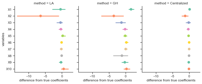
Although we tested the data sets with the state-of-art benchmark algorithm for centralized GLMM in R, the regression is not perfect for the ground truth coefficients we used to generate the data (Fig.2). So, it is also important to have the P-values of variables into consideration when interpreting the model. Thus, We made comparisons among centralized GLMM, Laplace method, and Gauss-Hermite method concerning the p-values of coefficients. Tables in the appendix captured the performance of different methods. Fig.3 shows the precision and recall results of centralized, Laplace, and Gauss-Hermite methods. Noted that we set our Gauss-Hermite approximation to 2-degree. See tables in Appendix (Tab.5, 6, 7).

The simulation results showed the federated Gauss-Hermite approximation performed better than the method based on Laplace approximation on every variable. Also, the federated Gauss-Hermite method achieved higher test power (Fig.4). When considering the convergence rates between the two approximation methods, both showed less convergence efficiency in Setting 7 and 8 (Tab.2). The result Indicates that more local sites and smaller sample sizes will make the federated GLMM more inefficient to converge. Also, GH approximation method will required more computation time compared with LA approximation. In sum, one-degree increase of the approximation function in LA with our developed GH method, GH outperformed LA methods for federated GLMM implementation.

We analyzed the data of COVID-19 electronic health records collected by Optum^® from February 2020 to January 28, 2021, from a network of healthcare providers. The dataset has been de-identified and based on HIPAA statistical de-identification rules and managed by Optum^® customer data user agreement. In this database, there are 56,898 unique positive tested COVID-19 patients. After removing the patients with missing data, the final cohort contains 4,531 patients who died and the rest population (41,781) survived. The database contains a regional variable with five levels (Midwest, Northwest, South, West, Others/unknown) to provide privacy-preserving area information to indicate where the samples were collected.

We have conducted a GLMM model (considering region-distinct random effect) using this dataset with the following predictors: age, gender, race, ethnicity, Chronic obstructive pulmonary disease (COPD), Congestive heart failure (CHF), Chronic kidney disease (CKD), Multiple sclerosis (MS), Rheumatoid arthritis (RA), LU (other lung diseases), High blood pressure (HTN), ischemic heart disease (IHD), diabetes (DIAB), Asthma (ASTH), obesity (Obese). Our proposed method with GH approximation performed the best with both the smallest Akaike information criterion (AIC) and Bayesian information criterion (BIC) according to the table of the goodness of fit (Tab.3). And the performance of different methods can be shown in (Tab.4).

We also compared the ROC curves (Fig.5) between our proposed GH method and centralized method to check their performance. And the result showed that GH approximation (AUC=0.72) outperforms the centralized method without regularization (AUC=0.68). Indicating GH-based GLMM method has better classification performance than the GLMM based on LA approximation. In our proposed model, it showed variables: Unknown race, Chronic kidney disease (CKD), Multiple sclerosis (MS), and other lung diseases (LU) are not significant to the mortality of COVID-19. The result of the regression is in the Appendix (Tab.8, 9, 10).

References

- [1] A. Telenti, X. Jiang, Treating medical data as a durable asset, Nature Genetics 52 (10) (2020) 1005–1010.
- [2] Hipaa privacy rule, 45 c.f.r. s 164 (2014).
- [3] L. Bonomi, X. Jiang, Linking temporal medical records using non-protected health information data, Statistical methods in medical research 27 (11) (2018) 3304–3324.
- [4] V. Janmey, P. L. Elkin, Re-identification risk in hipaa de-identified datasets: The mva attack, in: AMIA Annual Symposium Proceedings, Vol. 2018, American Medical Informatics Association, 2018, p. 1329.
- [5] L. Sweeney, J. S. Yoo, L. Perovich, K. E. Boronow, P. Brown, J. G. Brody, Re-identification risks in hipaa safe harbor data: A study of data from one environmental health study, Technology science 2017 (2017).
- [6] J. A. Nelder, R. W. Wedderburn, Generalized linear models, Journal of the Royal Statistical Society: Series A (General) 135 (3) (1972) 370–384.
- [7] N. R. Draper, H. Smith, Applied regression analysis, Vol. 326, John Wiley & Sons, 1998.
- [8] R. Zhu, C. Jiang, X. Wang, S. Wang, H. Zheng, H. Tang, Privacy-preserving construction of generalized linear mixed model for biomedical computation, Bioinformatics 36 (Supplement_1) (2020) i128–i135.
- [9] L. Xu, M. Jordan, On convergence properties of the EM algorithm for Gaussian mixtures, Neural computation 8 (1) (1996) 129–151.
- [10] Y. Wu, X. Jiang, J. Kim, L. Ohno-Machado, G rid binary lo gistic re gression (glore): building shared models without sharing data, Journal of the American Medical Informatics Association 19 (5) (2012) 758–764.
- [11] C. Luo, M. N. Islam, N. E. Sheils, J. Buresh, Y. Chen, dpql: a lossless distributed algorithm for generalized linear mixed model with application to privacy-preserving hospital profiling, medRxiv (2021).
- [12] X. Lin, N. E. Breslow, Bias correction in generalized linear mixed models with multiple components of dispersion, Journal of the American Statistical Association 91 (435) (1996) 1007–1016.
- [13] Q. Liu, D. A. Pierce, A note on gauss—hermite quadrature, Biometrika 81 (3) (1994) 624–629.
- [14] M. Kim, J. Lee, L. Ohno-Machado, X. Jiang, Secure and differentially private logistic regression for horizontally distributed data, IEEE Transactions on Information Forensics and Security 15 (2019) 695–710.
- [15] G. Broström, H. Holmberg, Generalized linear models with clustered data: Fixed and random effects models, Computational Statistics & Data Analysis 55 (12) (2011) 3123–3134.
Appendix A Supplementary proofs
A.1 Laplace approximation
Let us explain the Laplace approximation. Denote that
and one can see the log term inside the log-likelihood function that