On the Cardinality of Future Worldlines in Discrete Spacetime Structures

When we say a computable set we mean a set $A\subseteq\mathbb{N}$ for which there is an algorithm such that for any given natural number $n$, the algorithm can decide whether or not $n\in A$.¹⁵¹⁵ 15 We may use the terms computable and decidable interchangably depending on the context. Similarly, an $n$-ary relation $R$ is computable if it is computable as a set, that is, if for any given $n$-tuple $(x_{1},\ldots,x_{n})$, there is an algorithm which can decide whether or not $(x_{1},\ldots,x_{n})$ is in $R$. A set $A$ is countable if it is either finite or there is a one-to-one correspondence between $A$ and $\mathbb{N}$. If a countable set is infinite, then we call it a countably infinite set. If a set is not countable, we call it uncountable. Cantor’s theorem says that the cardinality of a set $A$ is strictly smaller than the cardinality of the set of all subsets of $A$.

Any countable set is in one-to-one correspondence with the set of natural numbers under an appropriate pairing function. The definition of a computable subset of naturals then generalizes to any countable set under a suitable pairing function. Let us now start by giving the notation for strings and trees.

Without loss of generality we may use the ordinal number notation and identify the ordinal 2, for instance, with the set of smaller ordinals $\{0,1\}$. A set $A\subseteq\mathbb{N}$ can be identified with its characteristic function $f:\mathbb{N}\rightarrow\{0,1\}$ such that $f(n)=1$ if $n\in A$, $f(n)=0$ otherwise. We represent the set of these functions as $2^{\mathbb{N}}$. This can be generalized to $n^{\mathbb{N}}$ for any natural number $n$. A set $A\subseteq\mathbb{N}$ codes an infinite 0-1 binary string if we take its characteristic function as a sequence of 0’s and 1’s so that if $n\in A$, then the $(n+1)$-th digit of the characteristic sequence of $A$ is 1, and it is 0 otherwise. So when we write $\sigma\subseteq A$ we mean $\sigma$ is an initial segment of $A$ as a sequence.

We say that a string $\sigma\in T$ is infinitely extendible in $T$ if there exists some $A\supseteq\sigma$ such that $A\in[T]$. A tree $T$ is perfect if every infinitely extendible string in $T$ has at least two incompatible extensions in $T$. If $\sigma,\tau\in T$ and $\sigma\subseteq\tau$ and there does not exist $\sigma^{\prime}$ with $\sigma\subseteq\sigma^{\prime}\subseteq\tau$ then we say that $\tau$ is an immediate successor of $\sigma$ in $T$ and $\sigma$ is the immediate predecessor of $\tau$ in $T$. Given the definitions above, we will view each event as a string, that is, an element of a tree, and view each worldline as a finite or infinite path. We give a discussion about this more in Section 2.3.

For a proof of this theorem, we refer the reader to [11] (pp. 129-130), as well as [29] (p. 53).

Since we work in Cantor space, we shall mention the compactness property of it. Although compactness can be provided by various forms, the most well known form is given by König’s lemma [22].

We shall now give some topological properties about finitely branching trees.

Note that when $\sigma$ isolates $A$, there are no incompatible infinite extensions of $\sigma$ in $T$. We remark the following proposition for the next subsection, although the proof is immediate from Cantor’s theorem.

The axioms of causal sets given in Section 1 describe a discrete spacetime structure on which a partial order is defined by causality. We said that each event is represented by an element of a tree. So if $\sigma$ and $\tau$ are two strings in $T$, and that $\sigma\subseteq\tau$, this means that the event denoted $\sigma$ is a cause of the event denoted by $\tau$ in the causal structure. Given any event $x$, the future light cone of $x$ is represented by a full $n$-ary tree $T$. So $T$ defines all possible events caused by $x$. Worldlines are defined by the collection of all paths on $T$, and a full $n$-ary tree is necessarily an uncountable set since it is perfect.¹⁷¹⁷ 17 For further discussion on how we define a tree for a light cone of an event, see Elaboration of III(a) in Section 2.3. But we ask under what conditions there could be less worldlines defined on $T$. Clearly, if all possible worldlines are terminating, then there must be only finitely many of them since there will always be an event in every worldline after which no event occurs.¹⁸¹⁸ 18 See the discussion at the end of Section 2.2 for more details. A more interesting worldline is that which is isolated by an event. An isolated path on $T$ describes a worldline which eventually stablizes and stops to split further. This corresponds to the following notion.

Now we will make use of the following results.

One consequence of this theorem concerns finite $\Pi^{0}_{1}$ classes.

The rest is just translating the results into the physical domain. We can argue for example that given any event $x$, if all worldlines extending $x$ are eventually deterministic, then there are countably many possible worldlines with respect to $x$. To see this, consider the future light cone of $x$, which is described by a tree $T$. If every member of $[T]$ is eventually deterministic—and so all isolated—then $[T]$ defines a discrete set. Thus $[T]$ is necessarily countable.

It also follows from Theorem 2 that if there are countably many future worldlines of an event $x$, then at least one of these worldlines is decidable.

On any tree $T\subseteq n^{\mathbb{N}}$, the number of finite paths can only be countable. This can be stated in terms of events and worldlines as follows.

We also claim that given an event $x$, if every future worldline of $x$ terminates, then the collection of future worldlines of $x$ is finite. This is because of the fact that if a worldline terminates, then it cannot constitute an infinite path, hence by the contrapositive of König’s lemma, the set of future events of $x$ is finite. Therefore, the set of future worldlines of $x$ must be finite given the hypothesis that every future worldline of $x$ terminates. Another proof of this fact relies on a computability theoretic approach. Any terminating future worldline of an event $x$ is a finite path which just happens to extend $x$. A finite path defines a finite set. Any finite set is computable. But there can only be countably computable sets since there are only countably many computable subsets of $\mathbb{N}$. This is because there are only countably many algorithms (or Turing machine programs) that can be written in a formal language.

One final thing before we conclude this section is to ask whether our analysis can be made on the many-worlds interpretation where the wave-function is always evolving deterministically and thus there are no probabilities. In this case, under the assumption that spacetime is discretized, the entire analysis reduces to answering the question whether there are countably or uncountably infinite orthogonal bases for this singular wave-function that encompasses all of the many-worlds. Such an investigation is out of the scope of this particular work, however, we invite interested colleagues to perform that study, which should yield qualitative differences between formulations of many-world interpretation where such a singular wave-function has countably infinite orthogonal bases in comparison to uncountably infinite ones.

In this part we elaborate on some of the assumptions given in Section 1 and then argue how the future light cone of an event is represented by a tree structure. In this representation, worldlines of infinite length form members of $\Pi^{0}_{1}$ classes (or they form paths on the corresponding computable tree). Hence, one can treat strings in a computable tree as spacetime events in light cones, and treat worldlines as paths on the tree. Collapsing strings in a perfect tree into the elements of the set may be thought of as applying a form of coarse graining of the causal set.

We now give some elaborations of the assumptions provided in Section 1 that need further explanation to complete the discussion on the representation of physical elements.

Given an event $x$, a split of at least two immediate effects of $x$ defines incomparable spacetime events (see Figure 2). In the MWI, thus, a split is usually considered as a way of defining distinct possible worlds.

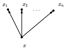
Hence the assumption given in II(d) ensures the existence of alternate/possible worldlines relative to any event. One may ask what would happen if there were mergings in the light cone of an event. It may be possible that two incomparable events may later merge into a single event and continue along the same worldline (see Figure 3). Even if separate worldlines merge into a single worldline at some point in the future—in which case the structure of causal sets could be represented by a directed acyclic graph—in our case one can just use trees to represent light cones. Furthermore, splitting and merging events will not have any effect on the cardinality of worldlines. The reason is the following. The number of paths from the beginning of the split to the merging region always is finite. Let us take Figure 3 as an illustration. A split occurs at event $b$ and a merging occurs at event $l$. Now there can only be finitely many events that are in the past of $l$ and the future of $b$. That is, there are finitely many $z$ such that $b\leq z\leq l$. We shall call the collection of such $z$’s a split-merge region. The number of paths that start with $b$ and end up with $l$ is clearly finite. This then has no effect on the number of worldlines in the future of $b$ if the future of $b$ contains infinitely many paths.

Possibility 1: The universe has no beginning. Assuming that the past of $x$ is eternal, future and past light cones of $x$ can be taken as two separate tree structures where one is just an inverted version of the other. So the same structure holds for both past and future light cones of an event $x$. That is, they are both infinite subsets of $n^{<\mathbb{N}}$.

Possibility 2: The universe has a beginning. In this case, the number of events that end up with $x$ is finite.

Assuming that the universe is indefinitely expanding, the number of future events of $x$ is greater than or equal to the number events in the past of $x$. So this means that, in the worst case, we can just work with the future light cone of $x$ to calculate the cardinality of the set of worldlines (past and future in complete) relative to $x$. The dominant factor without loss of generality can thus be assumed to come from the number of future worldlines of $x$.

We have not quite argued about how to form a computable tree of strings from events. Let $x$ be a spacetime event. The future light cone of $x$ can be formed as a tree $T\subseteq n^{<\mathbb{N}}$ for some natural number $n$ inductively as follows: We let $x$ be the empty string, hence the root of the tree. Let $\sigma\in T$ represents an event $y$. Every immediate effect $z_{i}$ of $y$ is defined by $\sigma*i$ in $T$.

The tree defined by the effects of an event $x$ constitutes a computable tree. This is in fact trivial since we really take the full tree $n^{<\mathbb{N}}$ to begin with, where $n$ is bounded by the spacetime region that a particle can travel from $x$ with a speed of light. So the tree $n^{<\mathbb{N}}$ consists of all immediate effects of $x$, all immediate effects of immediate effects of $x$, and so on. The future light cone of $x$ is then always computable and it basically corresponds to the full $n$-ary tree. By I(e), the immediate effects of any given event $x$ is bounded by the spacetime region through which light can travel from $x$ in least possible time tick. It is clear that the number of infinite paths on a full $n$-ary tree is uncountable since it is perfect (see Proposition 1).²⁰²⁰ 20 In [21], it was shown that as time tick $t$ increases, the number of possibilites grows exponentially. In [1], it was shown that every causal set dynamics typically yields an exponentially expanding universe. The way we define our tree and how it grows explonentially is compatible with this observation.

Given a spacetime event $x$, it should now be clear that the future light cone of $x$ is a full $n$-ary tree. The class of all infinite paths on this tree gives us an effectively closed set. So now properties about members of effectively closed sets and the topology of Cantor space that are given here can be interpreted as properties of light cones, worldlines and events in the way we described. Each future worldline is a path on the tree of effects of $x$.

References

- [1] Ahmed, M., Rideout, D. (2010). Indications of de Sitter spacetime from classical sequential growth dynamics of causal sets, Physical Review D, 81(8), 083528.
- [2] Belnap, N. (1992). Branching Space-Time, Synthese, 92(3), 385-434.
- [3] Belnap, N., Müller, T., Placek, T. (2021). New Foundations for Branching Space-Times, Studia Logica, 109(2), 239-284.
- [4] Bolognesi, T. (2011). Algorithmic Causets, J. Phys. Conf. Ser. 306, 012042.
- [5] Bombelli, L. (1987). Space-time as a causal set, PhD Thesis, Syracuse University.
- [6] Bombelli, L., Henson, J., Sorkin, R. D. (2009). Discreteness without symmetry breaking: a theorem, Mod Phys Lett. A24, 2579-2587.
- [7] Bombelli, L., Lee, J., Meyer, D., Sorkin, R. D. (1987). Space-time as a causal set, Phys. Rev. Lett. 59(5), 521-524.
- [8] Cantor, G. (1872). Ueber die Ausdehnung eines Satzes aus der Theorie der trigonometrischen Reihen, Mathematische Annalen, 5(1), 123-132.
- [9] Cenzer, D. (1999). Classes in Recursion Theory, in Handbook of Computability Theory, North-Holland, 37-39.
- [10] Deutsch, D. (1997). The fabric of reality: towards a theory of everything, Lane, London.
- [11] Diamondstone, D. E., Dzhafarov, D. D., Soare, R. I. (2010). Classes, Peano Arithmetic, Randomness, and Computable Domination, Notre Dame J. Formal Logic, 51, 127-159.
- [12] Dowker, F. (2006). Causal sets as discrete spacetime, Contemporary Physics, 47(1), 1-9.
- [13] Dowker, F., Zalel, S. (2017). Evolution of universes in causal set cosmology, Comptes Rendus Physique, 18(3-4), 246-253.
- [14] Dribus, B. F. (2018). Discrete Causal Theory Emergent Spacetime and the Causal Metric Hypothesis, Springer.
- [15] Earman, J. (2008). Chapter 10 Pruning Some Branches From “Branching Spacetimes”, Philosophy and Foundations of Physics, 4, 187-205.
- [16] Everett, H. (1957). Relative State Formulation of Quantum Mechanics, Rev. Mod. Phys. 29(3), 454-462.
- [17] Forrest, P. (1995). Is space-time discrete or continuous? - An empirical question, Synthese, 103(3), 327-354.
- [18] Healey, R. A. (1984). How Many Worlds?, Nous, 4, 591-616.
- [19] Hu, Y. (2013). The Causal Set Approach to Quantum Gravity, PhD Thesis, Imperial College London.
- [20] Kempf, A. (2010). Spacetime could be simultaneously continuous and discrete, in the same way that information can be, New Journal of Physics, 12(11), 115001.
- [21] Kleitman, D. J., Rothschild, B. L. (1975). Asymptotic enumeration of partial orders on a finite set, Transactions of the American Mathematical Society 205, 205-220.
- [22] König, D. (1926). Sur les correspondances multivoques des ensembles, Fundamenta Mathematicae, 8(1), 114-134.
- [23] Levichev, A. V. (1987). Prescribing the conformal geometry of a Lorentz manifold by means of its causal structure, Sov. Math. Dokl. 35, 452-455.
- [24] Linde, A., Vanchurin, V. (2010). How many universes are in the multiverse?, Phys. Rev. D, 81(8), 083525.
- [25] Malament, D. (1977). The Class of Continuous Timelike Curves Determines the Topology of Space-time, J. Math. Phys., 18, 1399-1404.
- [26] Masanes, L., Acin, A., Gisin, N. (2006). General properties of nonsignaling theories, Phys. Rev. A 73(1), 012112.
- [27] Meyer, D. A. (1988). The dimension of causal sets, PhD Thesis, Massachusetts Institute of Technology.
- [28] Müller, T. (2013). A generalized manifold topology for branching space-times, Philosophy of Science, 80(5), 1089-1100.
- [29] Nies, A. (2019). Computability and Randomness, Oxford University Press.
- [30] Norsen, T., Nelson, S. (2013). Yet Another Snapshot of Foundational Attitudes Toward Quantum Mechanics, arXiv: 1306.4646.
- [31] Reid, D. D. (2001). Discrete quantum gravity and causal sets, Canadian Journal of Physics, 79(1), 1-16.
- [32] Rideout, D. P., Sorkin, R. D. (1999). A Classical Sequential Growth Dynamics for Causal Sets, Phys. Rev. D: Particles and fields, 61(2), 024002.
- [33] Schlosshauer, M., Kofler, J., Zeilinger, A. (2013). A snapshot of foundational attitudes toward quantum mechanics, Studies in History and Philosophy of Science Part B: Studies in History and Philosophy of Modern Physics, 44(3), 222-230.
- [34] Sorkin, R. D., Gomberoff, A. (2005). Causal Sets: Discrete Gravity, in Lectures on Quantum Gravity, ed. Marolf, Donald, Springer, 305-327.
- [35] Surya, S. (2019). The causal set approach to quantum gravity, Living Reviews in Relativity, 22, Article no: 5.
- [36] Vanchurin, V. (2014). The Continuum of Discrete Trajectories in Eternal Inflation, Phys. Rev. D, 91(2), 023511.
- [37] Wallden, P. (2013). Causal Sets Dynamics: Review & Outlook, J. Phys.: Conf. Ser. 453, 012023.
- [38] Wütrich, C., Huggett, N. (2020). Out of Nowhere: The emergence of spacetime from causal sets, arXiv: 2009.02951.
- [39] Yamamoto, H. (1989). Discrete spacetime and Lorentz invariance, Nuclear Physics B - Proceedings Supplements 6, 154-156.