Geodesics in Jet Space.

Alejandro Bravo-Doddoli and Richard Montgomery Address: Alejandro Bravo-Doddoli: Dept. of Mathematics, UCSC, 1156 High Street, Santa Cruz, CA 95064 Email address: Abravodo@ucsc.edu Address: R. Montgomery: Dept. of Mathematics, UCSC, 1156 High Street, Santa Cruz, CA, 95064 Email address: rmont@ucsc.edu

Abstract.

The space $J^{k}$ of $k$ -jets of a real function of one real variable $x$ admits the structure of Carnot group type. As such, $J^{k}$ admits a submetry ( subRiemannian submersion) onto the Euclidean plane. Horizontal lifts of Euclidean lines (which are the left-translates of horizontal one-parameter subgroups) are thus globally minimizing geodesics on $J^{k}$ . All $J^{k}$ -geodesics, minimizing or not, are constructed from degree $k$ polynomials in $x$ according to [7],[8],[9], reviewed here. The constant polynomials correspond to the horizontal lifts of lines. Which other polynomials yield globally minimizers and what do these minimizers look like? We give a partial answer. Our methods include constructing an intermediate three-dimensional “magnetic” subRiemannian space lying between the jet space and the plane, solving a Hamilton-Jacobi (eikonal) equations on this space, and analyzing period asymptotics associated to period degenerations arising from two-parameter families of these polynomials. Along the way, we conjecture the independence of the cut time of any geodesic on jet space from the starting location on that geodesic.

Key words and phrases:

Carnot group, Jet space, minimizing geodesic, integrable system, Goursat distribution, subRiemannian geometry, Hamilton-Jacobi, period asymptotics

1. Introduction: Motivation, results, acknowledgement

It is a basic and important fact that lines in Euclidean space are globally minimizing geodesics. Not only are lines geodesics, but no matter how far out we travel along a line away from a point on the line, the corresponding line segment continues to minimize the distance between its end points. Contrast this with the case of geodesics on a cylinder, where most geodesics eventually fail to be minimizing. In the context of Carnot groups we can write down geodesic equations which describe most geodesics. (They miss the “abnormal” or “singular geodesics”. See [12].) The horizontal lines – the left translates of horizontal one-parameter subgroups - are globally minimizing geodesics. In the first non-trivial case, the Heisenberg group, the horizontal lines exhaust the set of globally minimizing geodesics. What happens for other Carnot groups? Are there any other globally minimizing geodesics besides the horizontal lines ?

The spaces $J^{k}=J^{k}(\mathbb{R},\mathbb{R})$ of $k$ -jets of a real function of a single real variable forms a family of $k+2$ -dimensional Carnot groups. (See [14].) $J^{k}$ is the unique Carnot group of its dimension Goursat type: its Lie bracket growth vector is $(2,3,4,\ldots,k+2)$ . $J^{1}$ is the well-known Heisenberg group and, as we just saw, has no global minimizers beyond the horizontal lines. $J^{2}$ is the Engel group [12] and has exactly one new global minimizer up to translation and scaling, this geodesic being the horizontal lift of the “Euler soliton” whose global minimality is established in [1, 2]. See the middle panel of figure 2.

Anzaldo-Meneses and Monroy-Peréz [7, 8, 9] showed that the subRiemannian geodesic flow on $J^{k}$ is completely integrable. In doing so they parameterized the space of all geodesics (modulo Carnot translations) by an open subset of the space of real polynomials $F(x)$ of degree $k$ (modulo translation $F(x)\mapsto F(x-x_{0})$ ).

Re-iterating, a geodesic is called globally minimizing if each of its compact subarcs realizes the distance between its endpoints. Our goal in this paper is to select out those degree $k$ polynomials which yield global minimizers on $J^{k}$ , $k>2$ .

We partially succeed. Theorem A below excludes most polynomials from yielding global minimizers. Theorem B establishes the existence of a previously unknown 8-dimensional family of global minimizers and characterizes them in terms of their polynomials. These two theorems are described in the next section, section 2. The question of finding an exact characterization of the global minimizers in terms of their polynomials remains open.

Our methods are three-fold. First, in section 4, for each choice of polynomial $F(x)$ we construct an intermediate 3-dimensional subRiemannian “magnetic space” denoted $\mathbb{R}^{3}_{F}$ which lies between $J^{k}$ and the Euclidean plane and we reduce most of our work to analysis on this space. Second, in section 5 we apply a Hamilton-Jacobi method (also known as the method of calibrations) to insure that our candidate globally minimizing geodesics actually globally minimize within a large open slab-like domain which contains them. Finally we are reduced to a detailed analysis of all the geodesics in the magnetic space which leave the slab-like domain to finish off the proof. In this last (exhausting) step which takes up section 7 we show that none of these competitor geodesics are simultaneously shorter and match endpoint conditions with our candidate geodesics.

1.1. Acknowledgement

It is an honor and a sadness to put forth this article in a Journal issue dedicated to Alexey Borisov. In addition to stating our gratitude to Borisov and condolences to his family and friends we would like to thank Andrei Ardentov, Gil Bor, Eero Hakavouri, Enrico Le Donne, Hector Sanchez-Morgado, Felipe Monroy-Perez, and Yuri Sachkov for e-mail conversations regarding the course of this work. We would also like to thank the three anonymous reviewers for their diligent work and useful suggestions. This paper was developed with the support of the scholarship (CVU 619610) from ”Consejo de Ciencia y Tecnologia” (CONACYT).

2. Set-up. Background. Theorems. Overview.

2.1. Set-up and Carnot group structure.

We say that smooth real-valued function $f(x)$ and $g(x)$ are equivalent up to order $k$ at $x_{0}$ if $f(x)-g(x)=O(|x-x_{0}|^{k+1})$ holds. Being equivalent to order $k$ is an equivalence relation on the space of germs of smooth functions at $x_{0}$ and an equivalence class is called a k-jet at $x_{0}$ . The $k$ -jet of a function $f$ at $x_{0}$ can be identified with its $k$ th order Taylor expansion of $f$ at $x_{0}$ and, as such, is determined by the list of its first $k$ derivatives at $x_{0}$ :

u_{0}=f(x_{0}),\qquad u_{j}=d^{j}f/dx^{j}(x_{0}):=f^{(j)}(x_{0}),j=1,\ldots,k.

By letting the base point and function vary we sweep out the $k$ -jet space $J^{k}$ , a $k+2$ -dimensional manifold with global coordinates $x$ and these $u_{j}$ ’s.

If we fix the function $f$ and let the independent variable $x$ vary, we get a curve $j^{k}f:\mathbb{R}\to J^{k}$ called the $k$ -jet of $f$ , sending $x\in\mathbb{R}$ to the $k$ -jet of $f$ at $x$ . In coordinates

(j^{k}f)(x)=(x,u_{k}(x),u_{k-1}(x),\ldots,u_{1}(x),u_{0}(x));\;\;u_{i}(x)=f^{(i)}(x)).

The $k$ -jet curve itself is everywhere tangent to the rank two distribution $D\subset TJ^{k}$ which is globally framed by the two vector fields

(1)

X_{1}=\frac{\partial}{\partial x}+\sum_{i=1}^{k}u_{i}\frac{\partial}{\partial u_{i-1}}\;\;\text{and}\;\;X_{2}=\frac{\partial}{\partial u_{k}}.

A subRiemannian structure on $J^{k}$ is defined by declaring these two vector fields to be orthonormal . In coordinates the subRiemannian metric is defined by restricting $ds^{2}=dx^{2}+du_{k}^{2}$ to $D$ . Now

\frac{d}{dx}j^{k}f(x)=X_{1}+f^{(k+1)}(x)X_{2}

so that the subRiemannian length $\ell$ of the curve $x\mapsto j^{k}f(x)$ , restricted to a finite interval $a\leq x\leq b$ is

\ell(j^{k}f|_{[a,b]})=\int_{a}^{b}\sqrt{1+(f^{(k+1)}(x))^{2}}dx.

The map $\pi:J^{k}\to\mathbb{R}^{2}$ defined by

\pi(x,u_{k},u_{k-1},\ldots,u_{0})=(x,u_{k})

defines a subRiemannian submersion (or submetry) onto the Euclidean plane. In other words, its restriction to each two-plane $D$ is an isometry onto the Euclidean plane with Euclidean metric $dx^{2}+du_{k}^{2}$ . This projection has an ‘inverse map’, the horizontal lift, on the level of curves. To understand the lift, rewrite $D$ as a Pfaffian system:

(2)

\displaystyle du_{i-1}-u_{i}dx

\displaystyle=

\displaystyle 0\;\;\;\text{with}\;1\leq i\leq k.

For example, the last of these equations, the one for $i=k$ , reads $du_{k-1}=u_{k}dx$ . Given a smooth curve $c(t)=(x(t),u_{k}(t))$ in the plane we associate to it the following horizontal lift equations

(3)

\displaystyle\dot{u}_{i}(t)

\displaystyle=u_{i+1}(x)\dot{x}(t),\qquad i=0,\ldots,k-1

which simply say that the curve $\gamma(t)=(x(t),u_{k}(t),u_{k-1}(t),\ldots,u_{0}(t))$ is horizontal and projects onto $c(t)$ . We call these curves $\gamma$ the horizontal lifts of our plane curve. The length of $\gamma$ and of $c$ over any compact time interval are equal. The horizontal lift $\gamma(t)$ is uniquely specified by the choice of initial condition, say $\gamma(0)$ , corresponding to the integration constants $u_{i}(0)$ ’s, $0\leq i<k$ . Any two horizontal lifts of the same curve differ by a Carnot translation. See below.

Our frame $\{X_{1},X_{2}\}$ generates a $k+2$ -dimensional nilpotent Lie algebra $\mathfrak{g}_{k}$ for which the following commuting relations hold:

X_{3}=[X_{2},X_{1}],X_{4}=[X_{3},X_{1}],\ldots,X_{k+2}=[X_{k+1},X_{1}],[X_{k+2},X_{1}]=0,

with

X_{3}={{\partial}\over{\partial u_{k-1}}},\;\;X_{4}={{\partial}\over{\partial u_{k-2}}},\;\ldots\;,\;\;X_{k+1}={{\partial}\over{\partial u_{1}}},\;\;X_{k+2}={{\partial}\over{\partial u_{0}}}.

All other Lie brackets $[X_{i},X_{j}]$ , $i,j>1$ are zero. This algebra is graded nilpotent:

\mathfrak{g}_{k}=V_{1}\oplus V_{2}\oplus\ldots V_{k+1},\;\;\;V_{1}=span\{X_{1},X_{2}\},\;\;\;V_{i}=span\{X_{i+1}\},\;\;2\leq i\leq k+1,

meaning that $[V_{i},V_{j}]\subset V_{i+j}$ . (Indeed $[V_{1},V_{j}]=V_{1+j}$ , and $[V_{i},V_{j}]=0$ if $i,j>1$ ). Thus $\mathfrak{g}_{k}$ forms a $(k+2)$ -dimensional graded nilpotent Lie algebra. The simply connected Lie group $G$ associated to any such algebra $\mathfrak{g}$ is, by definition, a Carnot group. The exponential map $\mathfrak{g}\to G$ is a diffeomorphism and provides $G$ with global coordinates under which the original vector fields are left-invariant and the multiplication is a ‘graded polynomial’ perturbation of vector addition, with the origin as the identity. Putting a Euclidean structure on its generating level 1 block $V_{1}$ induces a subRiemannian structure on the group, with distribution $D$ identified with $V_{1}$ left-translated about the group. It is this left-invariant subRiemannian structure which is typically studied when discussing Carnot groups.

2.2. Geodesic equations

Here is the advertised procedure ( [7, 8, 9]) for associating geodesics to polynomials in $x$ . Let $F(x)$ be any fixed polynomial in $x$ of degree $k$ or less. Solve:

(4)

\ddot{x}=-F(x)F^{\prime}(x),

for $x(t)$ , insisting that $x(t)$ also satisfy the energy constraint

(5)

\frac{1}{2}\dot{x}^{2}+\frac{1}{2}(F(x))^{2}=\frac{1}{2}.

The energy constraint is the arc length parameterization condition in disguise. Equation (4) is Newton’s equation for the potential $V(x)=\frac{1}{2}(F(x))^{2}$ . The left hand side of equation (5) is the conserved total energy for this Newton’s equation.

Having found such an $x(t)$ , next solve:

(6)

\dot{u}_{k}(t)=F(x(t)),

for $u_{k}(t)$ . The result is a plane curve $c(t)=(x(t),u_{k}(t))$ , $c:I\to\mathbb{R}^{2}$ . We can always take this interval $I$ to be the whole real line $I=\mathbb{R}$ . Horizontally lift this plane curve $c$ to form its horizontal lift $\gamma:\mathbb{R}\to J^{k}$ using the $k$ ‘triangular’ ODEs (3) of horizontal lifting. Due to the initial conditions going in to horizontal lift, this is not one curve, but a $k$ -parameter affine family of such curves parameterized by, for example $u_{i}(0)$ .

Background Theorem.

(See [7, 8, 9].) The above prescription yields a geodesic in $J^{k}$ parameterized by arclength. Conversely, any arc-length parameterized geodesic in $J^{k}$ can be achieved by this prescription applied to some polynomial $F(x)$ of degree $k$ or less.

We give an alternate proof of this theorem in Appendix A and a second alternative proof makes up the final paragraph of section 4.2.

The vector fields $X_{2},\ldots,X_{k+2}$ span a codimension one Abelian subalgebra $\mathfrak{h}$ of $\mathfrak{g}_{k}$ and the quotient space of $G=J^{k}$ by the corresponding Abelian group $H$ can be identified with the $x$ -axis. Translations by elements of $H$ correspond to translations of the coordinates $u_{i}$ . Since we have left the initial conditions of our geodesic equations free, the geodesics determined by a single polynomial $F(x)$ are determined up to left translation by elements of $H$ . To translate a geodesic in the $x$ -direction by an amount $x_{0}$ we must translate its polynomial : $F(x)\mapsto F(x-x_{0})$ . Translation by $x_{0}$ corresponds to left multiplication by $exp(x_{0}X_{1})$ .

The vector fields $X_{3},X_{4},\ldots,X_{k+2}$ form, in turn, an Abelian subalgebra $\mathfrak{k}\subset\mathfrak{h}\subset\mathfrak{g}$ , one which is, moreover, normal, being the commutator algebra $\mathfrak{k}=[\mathfrak{g},\mathfrak{g}]$ . The quotient of $J^{k}$ by this group is the Euclidean plane $\mathbb{R}^{2}$ and the projection $\pi:J^{k}\to\mathbb{R}^{2}$ described above corresponds to the quotient projection. On any Carnot group $G$ the analogous projection $G\to G/[G,G]\cong V_{1}$ is a a submetry. In this context the following principle is basic to all the work that follows.

Proposition 2.1.

If $M\to N$ is a submetry, meaning a submersion between subRiemannian submanifolds whose distributions have the same dimension, and with the property that the differential of the projection is an isometry between distribution planes, then the horizontal lift of a minimizing geodesic on $N$ is a minimizing geodesic on $M$ .

Proof.

Points on $N$ correspond to the fibers of $\pi$ upstairs on $M$ , a horizontal curve minimizes between two points of $N$ if and only if its lift minimizes between the fibers upstairs. In particular, the lift minimizes the subRiemannian distance between any two of its points. ∎

We apply this principle, that is, proposition 2.1 to our case of $\pi:J^{k}\to\mathbb{R}^{2}$ The geodesics on $\mathbb{R}^{2}$ are all known: they are the lines of the first paragraph of this paper and they are all global minimizers. Thus we have a corresponding family of globally minimizing geodesics on $J^{k}$ , the horizontal lifts of lines in the plane. These ‘horizontal lines” are precisely the curves of the form $t\mapsto h_{0}exp(tY)$ where $Y=aX_{1}+bX_{2}$ - the left translates by $h_{0}\in J^{k}$ of one-parameter subgroups lying in the first level $V_{1}$ . One checks without difficulty that these lines are in bijection with the constant polynomials $F(x)=b$ , in which case we take $a^{2}+b^{2}=1$ .

We are interested in the non-line geodesics, so those geodesics corresponding to non-constant polynomials. Multiply the energy equation (5) by $2$ to get

(7)

(\frac{dx}{dt})^{2}+F(x)^{2}=1,

for $x$ as a function of arclength $t$ . Since $\dot{x}^{2}\geq 0$ everywhere it follows that $x(t)$ must travel within one of the intervals on which $F(x)^{2}\leq 1$ . We call these the “Hill intervals” of $F(x)$ . There are at most $k$ such intervals since their endpoints must be solutions of the equation $F(x)^{2}=1$ . Once we choose one of these Hill intervals $I\subset\mathbb{R}$ for $x$ to travel in, the solution $x(t)$ is unique up to a time translation $x(t)\mapsto x(t-t_{0})$ . To summarize, every non-line geodesic is determined, up to a Carnot translation fixing the $x$ -axis and a time translation, by a choice of a degree $k$ polynomial $F(x)$ together with one of its Hill intervals $I$ . The endpoints of $I$ satisfy $F(x)=\pm 1$ and the interior points $x$ satisfy $F(x)^{2}<1$ .

Remark 2.1.

Given this bijection between geodesics on $J^{k}$ and the pairs $(F(x),I)$ , in the future we will specify a pair $(F(x),I)$ to define a geodesic $\gamma$ .

According to basic theory of one-degree of freedom classical mechanical systems, there are three possibilities for the $x$ -curve depending on whether or not the endpoints of its Hill interval are critical points of $F$ .

•

$x$ is periodic of some period $L$ : : $x(t+L)=x(t)$ . In this case neither endpoint of $x$ ’s Hill interval is a critical point of $F$ . These endpoints are referred to as the turning points of the solution.
•

$x$ is heteroclinic: $t\mapsto x(t)$ traverses its Hill interval exactly once as $t$ varies over $\mathbb{R}$ and does so in a strictly monotone fashion. As $t\to+\infty$ , $x(t)$ limits to one endpoint of its Hill interval, while as $t\to-\infty$ it limits to the other endpoint. In this case both endpoints of the Hill interval are critical points of $F$ . The solution has no turning point.
•

$x$ is homoclinic: $t\mapsto x(t)$ traverses its Hill interval twice while $t$ varies over $\mathbb{R}$ . Thus $x(t)$ limits to the same endpoint $x_{0}$ of the interval as $t\to\pm\infty$ . It hits the other endpoint $x_{1}$ once, at which instant $\dot{x}=0$ . We have $F^{\prime}(x_{0})=0$ while $F^{\prime}(x_{1})\neq 0$ where $\{x_{0},x_{1}\}$ are the endpoints of the Hill interval $I$ . The solution has a single turning point, $x=x_{1}$ .

In the heteroclinic case, we add one more dichotomy into the mix.

Definition 2.1.

A heteroclinic $x$ -curve with Hill interval $[x_{0},x_{1}]$ is said to be of turn-back type if $F(x_{0})\neq F(x_{1})$ , or equivalently, if $F(x_{0})F(x_{1})=-1$ . Otherwise, we say that the heteroclinic $x$ -curve is of direct type, in which case $F(x_{0})=F(x_{1})$ , or equivalently, if $F(x_{0})F(x_{1})=+1$ .

Definition 2.2.

A non-line geodesic is called x-periodic, heteroclinic, or homoclinic according to whether its $x$ -curve is periodic, heteroclinic or homoclinic. Similarly, we can speak of non-line geodesics as being heteroclinic of direct type or of turn-back type.

2.3. Main Results

Theorem A.

The following classes of geodesics in $J^{k}$ fail to be globally minimizing

•

(i) those which are $x$ - periodic.
•

(ii) those which are heteroclinic of turn-back type.

This theorem is proved in section 3. It is perhaps not a big surprise to a few experts who can prove both (i) and (ii) by the means by which we will prove item (ii).

What remains as possible globally minimizing geodesic candidates are homoclinic geodesics and the heteroclinic geodesics of direct type. Ardentov and Sachkov [1, 2] established the minimality of the homoclinic geodesics corresponding to $F(x)=ax^{2}-1,a>0$ when $k=2$ . Their work provided much of our inspiration. The plane curve for these geodesics will be called the Euler kink. (Other names for this plane curve are syntactrix and convict’s curve.) See the middle panel of figure 2. In subsection 2.4.3 near the end of this section we observe that the Euler kink continues to be globally minimal for all $k>2$ .

Theorem A also implies that any global minimizer which is not a line must be bi-asymptotic to ‘vertical lines’, meaning the horizontal lifts of lines of the form $x=const.$ . This fact is known to a few experts who understand the results of [11].

We proceed to our main new result.

Definition 2.3.

Call a real polynomial $F(x)$ a “seagull polynomial” if it is even, has maximum $1$ , has $0<F(0)<1$ and its only critical points are $0,\pm a$ where $F(\pm a)=1$ .

The graph of a seagull polynomial $F(x)$ is qualitatively that of a double well potential, reflected about the $x$ -axis. Since $a$ and $-a$ are double roots of $F(x)=1$ we have

(8)

1-F(x)=(x^{2}-a^{2})^{2}W(x)

with $W(x)>0$ and the only critical point of $W(x)=0$ is $x=0$ . The set of seagull polynomials of degree $2k$ forms a non-empy open set of dimension $k-1$ within the $k+1$ dimensional space of even polynomials of degree $2k$ . To get this count write $W(x)=a_{0}+a_{1}x^{2}+a_{2}x^{4}+\ldots+a_{k-2}x^{2(k-2)}$ , insist that $a_{0}$ and $a_{k-2}$ are positive, $0\leq a_{i}$ for $0<i<k_{2}$ and impose $a^{4}a_{0}<1$ , these last conditions imply that the set is open. Take the maximum point at $x=a$ as as an additional parameter.

Theorem B.

There is a non-empty $8$ dimensional open set of seagull polynomials of degree $18$ all of which yield globally minimizing geodesics of heteroclinic type on $J^{k}$ , for any $k\geq 18$ . See definition 7.2 for specifics regarding this set of polynomials. The Hill intervals $I$ of these geodesics are $[-x_{0},x_{0}]$ where $\pm x_{0}$ are the global maximum points of the seagull polynomial. (See figure 1.)

Refer to caption — Figure 1. The graph of a seagull polynomial (left panel) and the projection of its associated geodesic to the $(x,u_{k})$ plane.

The restriction to degree $18$ specified within definition 7.2 below occurs at only one step in our proof, the “ $Leg3$ ” step near the end. We are confident the theorem holds for all even degrees.

2.4. Miscellany.

2.4.1. Vertical lines as abnormal geodesics.

The geodesics for the constant polynomials $F=\pm 1$ form a special class of lines called “vertical lines” since they are given by $\dot{x}=0$ in the $(x,u_{k})$ plane. These are precisely the abnormal, or singular geodesics of $J^{k}$ . See [12], [13] or [4]. What makes them special in the metric category is that they are geodesics, independent of the variable inner product placed on the distribution planes. Theorem A implies that any non-line global minimizer is asymptotic to some vertical line as arclength $t\to+\infty$ and to a different vertical line as $t\to-\infty$ . These distinct lines have the same projection to the plane in the homoclinic case. This fact instantiates a general theorem found in [11].

See figure 2 for some representative examples.

See the rightmost panel of figure 2. In the turnback type we have $F(x_{1})=-F(x_{0})=\pm 1$ so that the shape of the plane curve looks like a giant $U$ according to equation (6) with $u_{k}$ reversing course as $t\to+\infty$ and traveling back the way it came from in the distant past. In the direct case, the asymptotic direction of motion of $u_{k}$ is the same in the distant past and distant future.

2.4.2. Scaling.

Carnot groups admit dilations $\delta_{h}:G\to G$ , $h\in\mathbb{R}\setminus\{0\}$ . The $\delta_{h}$ comprise a one-parameter group of automorphisms of $G$ which are also metric dilations: $d(\delta_{h}g,\delta_{h}y)=|h|d(g,y)$ . If $\gamma(t)$ is a geodesic parameterized by arc-length then so is

\gamma_{h}(t)=\delta_{\frac{1}{h}}\gamma(ht),

for any $h\neq 0$ . The Carnot dilation on $J^{k}$ is

\delta_{h}(x,u_{k},u_{k-1},\ldots,u_{0}):=(hx,hu_{k},h^{2}u_{k-1},h^{3}u_{k-2},\ldots,h^{k+1}u_{0}).

One verifies by direct computation, using the geodesic equations (4), (3), and (6), that if $F(x)$ is the polynomial yielding the non-line geodesic $\gamma(t)$ then $F_{h}(x):=F(hx)$ is the polynomial yielding the scaled non-line geodesic $\gamma_{h}(t)$ .

2.4.3. The other jet submetries.

We discussed the submetry $J^{k}\to\mathbb{R}^{2}$ . As a metric space, this $\mathbb{R}^{2}$ coincides with $J^{0}$ . These fit into a family of subRiemannian submersions to lower level jets, $\pi_{k,n}:J^{k}\to J^{n}$ with $n<k$ , so that $\pi=\pi_{k,0}$ ,

\pi_{k,1}:(x,u_{k},\dots,u_{1},u_{0})\mapsto(x,u_{k},u_{k-1}).

\vdots

\pi_{k,k-1}:(x,u_{k},\dots,u_{1},u_{0})\mapsto(x,u_{k},\dots,u_{2},u_{1}):=(x,v_{k-1},\dots,v_{1},v_{0}).

The last map $\pi_{k,k-1}$ realizes the quotient map $J^{k-1}\cong J^{k}/\exp(V_{k+2})$ . We identify this quotient space with $J^{k-1}$ by shifting the meaning of coordinates - the old $u_{0}$ has been projected out, and its derivative $u_{1}=du_{0}/dx$ is set to $v_{0}$ which now plays the role of the function whose jet we are taking when forming $J^{k-1}$ . The old $u_{k}$ continues its role as the ‘fiber coordinate’ of jet space, but this time now in the role of the $(k-1)$ th derivative of $v_{0}$ with respect to $x$ .

It follows from the basic principle, proposition 2.1, that a globally minimizing geodesic corresponding to some degree $n$ polynomial $F(x)$ persists by horizontal lift to yield a globally minimizing geodesic for all higher $k>n$ . In particular the geodesic which projects to the Euler kink continues to be a global minimizer for all $k>2$ .

3. Proof of theorem A

3.1. Case (i) the x-periodic case

Proposition 3.1.

Let $K$ be the following vector field

K=\sum_{i=0}^{k}\frac{x^{k-i}}{(k-i)!}\frac{d}{du_{i}},

then $K$ is a Killing vector field.

Proof.

First let us introduce a equivalence definition for a Killing vector field. Let $P_{1},P_{2}:T^{*}J^{k}\to\mathbb{R}$ be the momentum functions of the vector fields $X_{1},X_{2}$ , see [12] 8 pg. In terms of traditional cotangent coordinates $(x,u_{k},\cdots,u_{0},p_{x},p_{u_{k}},\cdots,p_{u_{0}})$ for $T^{*}J^{k}$ , we have

P_{1}=p_{x}+\sum_{j=0}^{k-1}u_{j+1}p_{u_{j}},\;\;P_{2}=p_{u_{k}}.

Then the Hamiltonian governing the geodesic on $J^{k}$ flow is $H=1/2(P_{1}^{2}+P_{2}^{2})$ . So $K$ is a Killing vector field if and only if its momentum function $P_{K}$ Poisson commute with $H$ , that is $\{P_{K},H\}=0$ . Then it is enough to prove that $\{P_{K},P_{1}\}=0$ and $\{P_{K},P_{2}\}=0$ , when

P_{K}=\sum_{i=0}^{k}\frac{x^{k-i}}{(k-i)!}p_{u_{i}}.

We have that $\{P_{K},P_{2}\}=0$ , since $P_{K}$ does not depend on $u_{k}$ . Then we will focus on the first bracket,

\begin{split}\{P_{K},P_{1}\}&=\{p_{x},\sum_{i=0}^{k}\frac{x^{k-i}}{(k-i)!}p_{u_{i}}\}+\{\sum_{j=0}^{k-1}u_{j+1}p_{u_{j}},\sum_{i=0}^{k}\frac{x^{k-i}}{(k-i)!}p_{u_{i}}\}\\ &=\sum_{i=0}^{k}p_{u_{i}}\{p_{x},\frac{x^{k-i}}{(k-i)!}\}+\sum_{j=0}^{k-1}\sum_{i=0}^{k}p_{u_{j}}\frac{x^{k-i}}{(k-i)!}\{u_{j+1},p_{u_{i}}\}\\ &=-\sum_{i=0}^{k-1}p_{u_{i}}\frac{x^{k-i-1}}{(k-i-1)!}+\sum_{i=0}^{k-1}\sum_{j=0}^{k}p_{u_{i}}\frac{x^{k-j}}{(k-j)!}\delta_{i+1,j},\\ \end{split}

where we used in the last line that the term from the first sum when $i=k$ does not depend on $x$ , then we can sum until $i=k-1$ . In the second sum we switch the place of $i$ and $j$ , also we used $\delta_{j+1,k-i}$ that is the Kronecker delta, $\delta_{i+1,k-j}$ is equal to $1$ when $i+1=j$ and zero otherwise, then

\begin{split}\{P_{K},P_{1}\}&=-\sum_{i=0}^{k-1}p_{u_{i}}\frac{x^{k-i-1}}{(k-i-1)!}+\sum_{i=0}^{k-1}p_{u_{i}}\frac{x^{k-i-1}}{(k-i-1)!}=0.\\ \end{split}

∎

The last proposition implies that the flow of $K$ generates a subRiemannian isometry. Now we are ready to prove case (i) from A.

Proof.

Case (i) from A: Let $\gamma$ be a geodesic for the polynomial $F(x)$ whose $x$ -curve $x(s)$ is periodic of period $L$ . Let $[x_{0},x_{1}]$ be the Hill interval for $x(s)$ so that $x_{0},x_{1}$ are turning points for $x$ . By performing an $x$ -translation we may assume that $x_{0}=0$ and by an $s$ -translation that $x(0)=0=x_{0}$ . Then $x(L/2)=x_{1}$ and $x(L)=0$ . We claim that $\gamma(L)$ is conjugate to $\gamma(0)$ along $\gamma$ .

Next, observe that at the turning points $s=0,L/2,L,3L/2,2L,\ldots$ of the $x$ -curve we have $\dot{x}(s)=0$ so that $\gamma$ is tangent to the vertical direction ${{\partial}\over{\partial u_{k}}}$ at these times. In particular, by reversing directions if necessary, we have that $\dot{\gamma}(0)=\dot{\gamma}(L)={{\partial}\over{\partial u_{k}}}$ . Now consider the following two Jacobi fields for $\gamma$ :

\begin{split}W_{1}(s)&=K\text{ restricted to }\gamma,\\ W_{2}(s)&=\dot{\gamma}(s).\end{split}

Since $x(kL)=0$ we have that $W_{1}(jL)={{\partial}\over{\partial u_{k}}}$ , $j=0,1,2,\ldots$ so that $W_{1}(0)=W_{2}(0)=W_{1}(L)=W_{2}(L)$ . Since the space of Jacobi fields is a linear space so that $J:=W_{1}-W_{2}$ is again a Jacobi field for $\gamma$ and this field now vanishes at every $s=jL,j=0,1,\ldots$ . In the interior of the interval $(0,L)$ the field $J$ is not identically zero since $\dot{x}(s)\neq 0$ for $0<s<L/2$ . It follows that $J$ contributes at least $1$ to the nullity of the Hessian of the action - so the squared length functional $\int_{0}^{s}\frac{1}{2}\|\dot{\gamma}(s)\|^{2}ds$ - thus establishing that the times $s=L,2L,\ldots$ are conjugate times to $s=0$ along $\gamma$ . It follows by standard calculus of variations that the geodesic $\gamma$ fails to minimize beyond $L$ . ∎

3.2. Case (ii) : the heteroclinic turn-back case.

Our proof relies on the method of blowing-down geodesics as explained by Hakavuouri-Le Donne [11]. Suppose that $\gamma:\mathbb{R}\to G$ is a rectifiable curve in a Carnot group $G$ . For $h\in\mathbb{R}^{+}$ form

\gamma_{h}(t)=\delta_{\frac{1}{h}}\gamma(ht),

where $\delta_{h}:G\to G$ is the Carnot dilation. One easily checks that if $\gamma$ is a geodesic then so is $\gamma_{h}$ for any $h>0$ .

Definition 3.1.

A blow-down of $\gamma$ is any limit curve $\tilde{\gamma}=\lim_{k\to\infty}\gamma_{h_{k}}$ where $h_{k}\in\mathbb{R}$ is any sequence of scales tending to infinity with $k$ , and the limit being uniform on compact sub-intervals.

Hakavouri and LeDonne [11] prove the following lemma:

Lemma 3.1.

If $\gamma$ is globally minimizing geodesic parameterized by arclength then any one of its blow-downs $\tilde{\gamma}$ is also a globally minimizing geodesic parameterized by arc-length.

Proof.

Proof of case (ii) from A: The projection $\pi$ to the $(x,u_{k})$ plane of a heteroclinic turnback geodesic $\gamma$ lies between two vertical lines $x=x_{0}$ and $x=x_{1}$ and its height $u_{k}$ achieves a global maximum or minimum at some point $P$ in between these lines. (See the right panel of figure 2.) The geodesic $\gamma$ is asymptotic to of one of these vertical lines as $t\to-\infty$ and to the other as $t\to+\infty$ . Using a time translation if needed, we may assume that the extremal point $P$ occurs when $t=0$ and by using a translation we can assure that $P=0\in J^{k}$ . And by using the dilation $\delta_{-1}$ we can assure that $P$ is a global minimum point for $u_{k}$ , so that $u_{k}>0$ everywhere else along the curve. Let $[x_{0},x_{1}]$ be the geodesic’s Hill interval. Then, upon dilating we have that $\pi\circ\gamma_{h}$ lies between the two vertical lines $x=x_{0}/h$ and $y=x_{1}/h$ and is asymptotic to one of them as $t\to-\infty$ and the other as $t\to+\infty$ , while for all $\gamma_{h}(0)=0$ . It follows that any blow-down of $\gamma$ consists of the horizontal lift of the vertical ray $x=0,u_{k}\geq 0$ , traversed twice, once coming in from infinity, hitting zero, then reversing course and heading back out to infinity. But a ray, traversed twice is not a minimizing geodesic, since it is not smooth curve on the $x-u_{k}$ plane (any geodesic on a Riemannian manifold is smooth), and neither are any of its horizontal lifts. So $\gamma$ cannot itself cannot be a globally minimizing geodesic, for if it were, the Hakavuori-Le Donne lemma would imply that the vertical ray, traversed there and back, is a globally minimizing geodesic. But a curve which retraces its own path is never a minimizing geodesic: simply chop off and shorten the path by stopping before the turn-around point $P$ and turn back earlier. ∎

4. Setting up for theorem B.

4.1. The intermediate Magnetic space

As a first step towards proving theorem B we factor the subRiemannian submersion $\pi:J^{k}\to\mathbb{R}^{2}$ into the product of two subRiemannian submersions:

(9)

\pi=pr\circ\pi_{F},

where the target of $\pi_{F}$ is an intermediate 3-dimensional subRiemannian space denoted by $\mathbb{R}^{3}_{F}$ whose geometry depends on the choice of polynomial $F(x)$ and which we refer to as a ‘magnetic subRiemannian structure’. Thus we will have subRiemannian submersions

\lx@xy@svg{\hbox{\raise 2.5pt\hbox{\kern 8.71355pt\hbox{\ignorespaces\ignorespaces\ignorespaces\hbox{\vtop{\halign{\entry@#!@&&\entry@@#!@\cr&&\crcr}}}\ignorespaces{\hbox{\kern-8.71355pt\raise 0.0pt\hbox{\hbox{\kern 0.0pt\raise 0.0pt\hbox{\hbox{\kern 3.0pt\raise-2.5pt\hbox{$\textstyle{J^{k}\ignorespaces\ignorespaces\ignorespaces\ignorespaces}$}}}}}}}\ignorespaces\ignorespaces\ignorespaces\ignorespaces{}{\hbox{\lx@xy@droprule}}\ignorespaces\ignorespaces\ignorespaces{\hbox{\kern 13.16843pt\raise 5.00972pt\hbox{{}\hbox{\kern 0.0pt\raise 0.0pt\hbox{\hbox{\kern 3.0pt\hbox{\hbox{\kern 0.0pt\raise-1.00417pt\hbox{$\scriptstyle{\pi_{F}}$}}}\kern 3.0pt}}}}}}\ignorespaces{\hbox{\kern 32.71355pt\raise 0.0pt\hbox{\hbox{\kern 0.0pt\raise 0.0pt\hbox{\lx@xy@tip{1}\lx@xy@tip{-1}}}}}}{\hbox{\lx@xy@droprule}}{\hbox{\lx@xy@droprule}}{\hbox{\kern 32.71355pt\raise 0.0pt\hbox{\hbox{\kern 0.0pt\raise 0.0pt\hbox{\hbox{\kern 3.0pt\raise-2.5pt\hbox{$\textstyle{\mathbb{R}^{3}_{F}\ignorespaces\ignorespaces\ignorespaces\ignorespaces}$}}}}}}}\ignorespaces\ignorespaces\ignorespaces\ignorespaces{}{\hbox{\lx@xy@droprule}}\ignorespaces\ignorespaces\ignorespaces{\hbox{\kern 60.13489pt\raise 5.1875pt\hbox{{}\hbox{\kern 0.0pt\raise 0.0pt\hbox{\hbox{\kern 3.0pt\hbox{\hbox{\kern 0.0pt\raise-0.8264pt\hbox{$\scriptstyle{pr}$}}}\kern 3.0pt}}}}}}\ignorespaces{\hbox{\kern 76.72261pt\raise 0.0pt\hbox{\hbox{\kern 0.0pt\raise 0.0pt\hbox{\lx@xy@tip{1}\lx@xy@tip{-1}}}}}}{\hbox{\lx@xy@droprule}}{\hbox{\lx@xy@droprule}}{\hbox{\kern 76.72261pt\raise 0.0pt\hbox{\hbox{\kern 0.0pt\raise 0.0pt\hbox{\hbox{\kern 3.0pt\raise-2.5pt\hbox{$\textstyle{\mathbb{R}^{2}_{x,u_{k}}}$}}}}}}}\ignorespaces}}}}\ignorespaces,

if $x,y,z$ are coordinates on this intermediate space then the distribution $D_{F}$ on $\mathbb{R}^{3}_{F}$ is defined by the single Pfaffian equation:

(10)

D_{F}:dz-F(x)dy=0,

while the metric $ds^{2}$ on the two-planes $D_{F}$ is defined by

(11)

ds^{2}=(dx^{2}+dy^{2})|_{D_{F}},

and the projection to the plane $\mathbb{R}^{2}$ by

pr(x,y,z)=(z,y)=(x,u_{k}).

Before we describe the projection we pause to explain why we’ve used the term “magnetic”. The motion of a particle of charge $e$ moving non-relativistically in the Euclidean plane under the influence of a magnetic field of strength $B(x,y)$ orthogonal to the plane is given by $\ddot{c}=eB(c){\mathbb{J}}\dot{c}$ . Let $A=A_{1}(x,y)dx+A_{2}(x,y)dy$ be a vector potential for $B$ , meaning that $dA=Bdx\wedge dy$ . The Hamiltonian system on $T^{*}\mathbb{R}^{2}$ having Hamiltonian $H=\frac{1}{2}(p_{x}-eA_{1}(x,y))^{2}+(p_{y}-eA_{2}(x,y))^{2}$ generates the motion of this particle. (See, eg [10].) Introduce a third variable $z$ with conjugate momentum $p_{z}$ so that $H$ becomes $H=\frac{1}{2}(p_{x}-p_{z}A_{1}(x,y))^{2}+(p_{y}-p_{z}A_{2}(x,y))^{2}$ on $T^{*}\mathbb{R}^{3}$ . This is the subRiemannian kinetic energy for the subRiemannian structure on $\mathbb{R}^{3}$ defined by the distribution $D=ker(dz-A)$ with inner product $dx^{2}+dy^{2}|_{D}$ . Since $H$ is independent of $z$ we have that $p_{z}$ is constant along trajectories and we identify this constant with the charge $e$ . (See, eg [12].) We call any subRiemannian structure of this form on $\mathbb{R}^{3}$ a magnetic subRiemannian structure. Our $\mathbb{R}^{3}_{F}$ is such a structure with $A=F(x)dy$ .

To construct the projection $\pi_{F}$ expand out

F(x)=\Sigma\frac{a_{j}}{j!}x^{j}

and use the alternate coordinates $\theta_{j}$ for $J^{k}$ as those described in [7] and [8] with an index swapping and sign change:

\theta_{0}=u_{k},\cdots,\;\theta_{j}=\sum_{i=0}^{j}(-1)^{i}\frac{x^{j-i}}{(j-i)!}u_{k-i},\cdots,\;\theta_{k}=\sum_{i=0}^{k}(-1)^{i}\frac{x^{k-i}}{(k-i)!}u_{k-i},

(The $u_{j}$ of Monroy-Perez and Anzaldo Meneses are not exactly the same as ours, rather they are related to ours by an index swapping and a sign change. To be precise, that is, if $v_{j}$ denotes the $u_{j}$ in [7] then $v_{j}=(-1)^{j}u_{k-j}$ .)

Written in $\theta$ -coordinates our frame for the distribution $D$ on $J^{k}$ is

X_{1}={{\partial}\over{\partial x}},\qquad X_{2}={{\partial}\over{\partial y}}+\sum\frac{x^{j}}{j!}{{\partial}\over{\partial\theta_{j}}},

where $y=u_{k}=\theta_{0}.$

Define $\pi_{F}:J^{k}\to\mathbb{R}^{3}$ to be linear in the $\theta$ coordinates and with coefficients constructed from the scaled coefficients $a_{j}$ of our chosen $F(x)$ :

\displaystyle\pi_{F}(x,\theta_{0},\theta_{1},\ldots,\theta_{k})=(x,\theta_{0},\sum_{i=0}^{k}a_{i}\theta_{i}):=(x,y,z)

in the original coordinates the projection looks as

\begin{split}\pi_{F}(x,u_{k},u_{k-1},\ldots,u_{0})=(x,u_{k},\sum_{i=0}^{k}(-1)^{k-i}u_{i}\frac{d^{k-i}F}{dx^{k-i}}(x)).\\ \end{split}

From the linearity of $\pi_{F}$ in these coordinates we easily compute

\pi_{F*}X_{1}={{\partial}\over{\partial x}}\;\;\text{and}\;\;\pi_{F*}X_{2}={{\partial}\over{\partial y}}+F(x){{\partial}\over{\partial z}},

which is an orthonormal horizontal frame for the subRiemannian structure $\mathbb{R}^{3}_{F}$ as defined by equations (10) and (11), establishing the factorization (9).

4.2. Magnetic geodesics.

The subRiemannian kinetic energy Hamiltonian for $\mathbb{R}^{3}_{F}$ is

H_{F}=\frac{1}{2}p_{x}^{2}+\frac{1}{2}(p_{y}+F(x)p_{z})^{2}.

The projection $(x(s),y(x),z(s))$ to $\mathbb{R}^{3}_{F}$ of any solution curve

(x(s),y(x),z(s),p_{x}(s),p_{y}(s),p_{z}(s))\in T^{*}\mathbb{R}^{3}_{F},

to Hamilton’s equations for $H_{F}$ is a geodesic. The geodesic is parameterized by arc-length if $H_{F}=1/2$ . Since no $y$ ’s or $z$ ’s occur in $H_{F}$ , the time derivatives of the momenta $p_{y},p_{z}$ are zero so we have that

p_{y}=a,\;\;\text{and}\;\;p_{z}=b

with $a$ and $b$ constant.

It makes sense to call $p_{x}=p$ momentum for $x$ , we then have

H_{F}=\frac{1}{2}p^{2}+V(x),\qquad V(x)=\frac{1}{2}(a+bF(x))^{2}.

Hamilton’s equations for the pair $(x,p)$ are identical to the 1st geodesic equation, equations (4) and (5) upon replacing $F$ by $G=a+bF$ . Thus the $x$ -component of our geodesic is, following definition 4, an $x$ -curve for $G$ .

Definition 4.1.

The pencil of the polynomial $F$ is the two-dimensional linear space of polynomials having the form

(12)

G(x):=a+bF(x),

where $a,b$ are arbitrary real constants.

What about the remaining components $y(s),z(s)$ of our geodesic? Using that $H_{F}=\frac{1}{2}(p^{2}+P_{y}^{2})$ with $P_{y}=p_{y}+p_{z}F(x)=a+bF(x)=G(x)$ and writing out Hamilton’s equations for $y$ and $z$ we get

(13)

\begin{split}\dot{y}&=G(x),\\ \dot{z}&=G(x)F(x).\\ \end{split}

The first equation is equation (6) after replacing $F$ by $G=a+bF$ . The second equation, upon substituting in the first, says that $\dot{z}-F(x)\dot{y}=0$ , which simply says that $(x(s),y(s),z(s))$ is the horizontal lift of the plane curve

(x(s),y(s))=(x(s),u_{k}(s)).

Since $\pi_{F}$ is a subRiemannian submersion, the horizontal lift of any $\mathbb{R}^{3}_{F}$ -geodesic for $F$ is a geodesic on $J^{k}$ . Horizontal lift is given by lifting the plane curve $(x(s),y(s))=(x(s),u_{k}(s))$ , which is to say, by equations (3). We have proven

Lemma 4.1.

Every $\mathbb{R}^{3}_{F}$ geodesic is the $\pi_{F}$ -projection of a geodesic in $J^{k}$ corresponding to some $G$ in the pencil of $F$ . Conversely, the horizontal lifts to $J^{k}$ of $\mathbb{R}^{3}_{F}$ -geodesics are precisely those geodesics corresponding to polynomials in $F$ ’s pencil.

Remark. As an immediate corollary to the lemma we get:

Proof of Theorem Background Theorem (“Background Theorem”). Take $a=0,b=1$ so that $G=F$ . The lift of the geodesic in $\mathbb{R}^{3}_{F}$ corrresponding to $G=G$ is a $J^{k}$ -geodesic.

4.3. Periods I

Proposition 4.1.

Let $c(t)=(x(t),y(t),z(t))$ in $\mathbb{R}^{3}_{F}$ be the projection of an $x$ -periodic geodesic in $J^{k}$ having corresponding polynomial $G=a+bF$ and Hill interval $[x_{0},x_{1}]$ . (Recall that $G(x_{0})^{2}=G(x_{1})^{2}=1$ .) Then the $x$ -period is

(14)

L=2\int_{x_{0}}^{x_{1}}\frac{dx}{\sqrt{1-G^{2}(x)}},

and is twice the time it takes the $x$ -curve to cross its Hill interval exactly once. After one period the changes $\Delta y=y(t_{0}+L)-y(t_{0})$ and $\Delta z=z(t_{0}+L)-z(t_{0})$ undergone by $y$ and $z$ are given by

\Delta y=2\int_{x_{0}}^{x_{1}}\frac{G(x)dx}{\sqrt{1-G^{2}(x)}},\;\Delta z=2\int_{x_{0}}^{x_{1}}\frac{F(x)G(x)dx}{\sqrt{1-G^{2}(x)}}.

Proof.

Along any arc of $c$ for which $x(t)$ is monotonic we can re-express the curve as a function of $x$ instead of $t$ using $(dx/dt)^{2}=1-G(x)^{2}$ or $\frac{dx}{dt}=\pm\sqrt{1-G(x)^{2}}$ . Note the sign of the $\pm$ changes each time $x(t)$ reflects off of an endpoint of its Hill interval. Then, as is standard in mechanics, the total period $L$ is twice the time $\Delta t$ required to cross the Hill interval. We have

\Delta t=\int dt=\int\frac{dt}{dx}dx=\int_{x_{0}}^{x_{1}}\frac{1}{\sqrt{1-G^{2}(x)}}dx.

For the other two periods use that the differential equations (13) assert that $dy=G(x(t))dt$ and $dz=F(x(t))G(x(t))dt$ . Choose $x(t)$ so that $x(0)=x_{0}$ . Then $x(L/2)=x_{1}$ . and $x(L/2+t)=x(L/2-t)$ . It follows that the change in $y$ and $z$ over a full period is twice their change over a half-period. Since $dt=\frac{1}{\sqrt{1-G^{2}(x)}}dx$ on the first period we get the result provided we start at $x_{0}$ at time $t=0$ . To see that the result of $\Delta y$ is independent of the starting point, differentiate $y(t+L)-y(t)$ with respect to $t$ . The derivative is $G(x(t+L))-G(x(t))$ . But $x(t+L)=x(t)$ so this derivative is zero. The same proof works for $\Delta z$ . ∎

Remark. The above equation for $L$ is the well known formula for the period of a one-freedom degree mechanical system. Where $x_{0}$ and $x_{1}$ are the points when the potential energy is equal to total energy of the system, $F(x)^{2}=1$ , and we use the reversibility of the system, if $x(t)$ is a solution to the Newton’s equation then $x(-t)$ is too, to assure that the time that takes to the particle to travel from $x_{0}$ to $x_{1}$ is equal to the one from $x_{1}$ to $x_{0}$ , then the period $L$ is equal to the time that takes to the particle to come back to the initial point and is independent of the initial point and initial time.

Remark. $\Delta y$ and $\Delta z$ are also independent of $t_{0}$ , which is to say, of the initial point of the curve.

5. Calibrations: a Hamilton-Jacobi method for local minimality

Suppose $H:T^{*}Q\to\mathbb{R}$ is a Hamiltonian on some standard phase space $T^{*}Q$ . The associated time-dependent Hamilton-Jacobi equation is the PDE

H(q,dS(q))=const,

to be solved for a function $S:Q\to\mathbb{R}$ . For lines in Euclidean geometry, we take $Q=\mathbb{R}^{n}$ , $H(q,p)=\frac{1}{2}\|p\|^{2}$ , the Hamiltonian of a free particle, and the constant to be $1/2$ . Then the Hamilton-Jacobi PDE reads $\|\nabla S\|=1$ and in this guise is often called the eikonal equation – the equation of light rays. The integral curves of the gradient flow, $\dot{q}=\nabla S(q)$ , are straight lines. A typical solution $S$ has the form $S(q)=dist(q,C)$ where $C\subset\mathbb{R}^{n}$ is a closed set. All of this extends to the Hamilton-Jacobi equation associated to the geodesic equations in Riemannian and in subRiemannian geometry. See pp 14-15 of [12] for details.

In the subRiemannian case the Hamilton-Jacobi equation associated to geodesic flow is called the “eikonal equation” following the usage of geometric optics. This equation reads

(15)

\|\nabla_{hor}S\|=1,

where $\nabla_{hor}$ is the horizontal derivative of $S:Q\to\mathbb{R}$ , that is, $\nabla_{hor}S$ is the unique horizontal vector field satisfying, for every $q$ in $Q$ ,

\langle\nabla_{hor}S,v\rangle_{q}=dS(v),\;\;\text{for every}\;v\in D_{q}.

Where $\langle\;,\;\rangle$ is the subRiemannian inner product.

A more careful definition of “globally minimize” is in order

Definition 5.1.

A. Let $\Omega\subset Q$ be a domain within a subRiemannian manifold $Q$ and $I\subset\mathbb{R}$ a closed bounded interval. We say that $c:I\to\Omega$ globally minimizes within $\Omega$ if whenever $\tilde{c}:J\to\Omega$ is any smooth horizontal curve lying in $\Omega$ and sharing endpoints with $c$ , then $\ell(c)\leq\ell(\tilde{c})$ .

B. If the interval $I\subset\mathbb{R}$ is not closed and bounded then we say that $c:I\to\Omega$ is “globally minimizing within $\Omega$ ” if every closed bounded sub-arc $c([t_{0},t_{1}])$ of $c$ , $t_{0},t_{1}\in I$ is globally minimizing within $\Omega$ in the sense of A.

Remark 5.1.

In part A of the definition we could have replaced “any smooth horizontal curve lying in $\Omega$ by “any continuous curve lying in $\Omega$ ” without changing the meaning. The reason is that the subRiemannian length functional $c\mapsto\ell(c)$ satisfies the property that if $\ell(c)<\infty$ then $\ell(c)=\lim\ell(C_{i})$ where the $C_{i}\to c$ is any sequence of smooth paths $C_{i}$ which converge to $c$ in either the $H^{1}$ or the Lipshitz sense. See [12] for details.

Proposition 5.1.

If $S$ is a $C^{2}$ solution of the eikonal equation (15) defined on a simply connected domain $\Omega\subset Q$ , then the integral curves of its horizontal gradient flow $\dot{c}=\nabla_{hor}S(c)$ are subRiemannian geodesics which globally minimize within the domain $\Omega$ .

Proof.

Let $A,B$ be the shared endpoints of our competing curves $c,\tilde{c}$ . Then Stokes’s theorem imply:

\int_{c}dS=\int_{\tilde{c}}dS=S(B)-S(A).

But for any smooth curve $\gamma$ in $\Omega$ we have that

\int_{\gamma}dS=\int\langle\nabla S,\dot{\gamma}\rangle dt\leq\int_{\gamma}\|\dot{\gamma}\|\|\nabla_{hor}S\|dt=\int_{\gamma}\|\dot{\gamma}\|dt=\ell(\gamma).

Equality holds in this series of inequalities if and only if $\dot{\gamma}=f\nabla_{hor}S$ for some positive scalar $f$ , that is, if and only if $\gamma$ is a reparameterization of an integral curve of $\nabla_{hor}S$ . Our curve $c$ is such an integral curve, that is, $\dot{c}(t)=(\nabla_{hor}S)_{c(t)}$ , then

dS(\dot{c})=\langle\nabla_{hor}S,\dot{c}\rangle=\langle\nabla_{hor}S,\nabla_{hor}S\rangle=1.

Any other competing curve lying in $\Omega$ satisfies

dS(\dot{\tilde{c}})=\langle\nabla_{hor}S,\dot{\tilde{c}}\rangle<\|\dot{\tilde{c}}\|

on an open set of points, it is a strictly inequality since $\tilde{c}$ is different of $c$ at least on an open set, so the above equality becomes

(16)

\ell(c)=S(B)-S(A)<\ell(\tilde{c}),

where $\ell$ is the subRiemannian length. ∎

In the particular case where $Q=\mathbb{R}^{3}_{F}$ we can simplify the eikonal equation. Recall the subRiemannian structure on $\mathbb{R}^{3}_{F}$ . (See equations (10, 11).) Also recall that we are now denoting our coordinates on $\mathbb{R}^{3}_{F}$ by $x,y,z$ . (See the beginning of subsection 6.3.) Take any $S=S(x,y,z)$ , compute

dS={{\partial S}\over{\partial x}}dx+{{\partial S}\over{\partial y}}dy+{{\partial S}\over{\partial z}}dz,

use that $dz=F(x)dy$ on horizontal planes to see that

dS|_{D}={{\partial S}\over{\partial x}}dx|_{D}+({{\partial S}\over{\partial y}}+{{\partial S}\over{\partial z}}F(x))dy|_{D}.

Since $dx,dy$ form an orthonormal coframe for $D^{*}$ we have

(17)

\nabla_{hor}S={{\partial S}\over{\partial x}}E_{1}+({{\partial S}\over{\partial y}}+{{\partial S}\over{\partial z}}F(x))E_{2},

where

E_{1}={{\partial}\over{\partial x}},E_{2}={{\partial}\over{\partial y}}+F(x){{\partial}\over{\partial z}},

is the orthonormal frame dual to $dx,dy$ . The eikonal equation for $S$ then reads

(18)

({{\partial S}\over{\partial x}})^{2}+(({{\partial S}\over{\partial y}}+{{\partial S}\over{\partial z}}F(x))^{2}=1.

Take the ansatz

(19)

S(x,y,z)=bz+ay+f(x),

for a solution $S$ to be associated to the polynomial $G=a+bF$ in the pencil of $F$ . Then eq (18) becomes

(20)

f^{\prime}(x)^{2}+(a+bF(x))^{2}=1,

and the associated horizontal gradient flow vector field is

(21)

\nabla_{hor}S=f^{\prime}(x)E_{1}+(a+bF(x))E_{2}.

Compare these equations with that of the geodesic equations for $G$ . The $x$ -curve for $G$ satisfies the energy equation:

\dot{x}^{2}+(a+bF(x))^{2}=1,

while the $u_{k}=y$ equation for $G$ ’s geodesic is

\dot{y}=a+bF(x).

Solve the energy equation to get

\dot{x}=\pm\sqrt{1-(a+bF(x))^{2}}.

Conclude that the horizontal gradient flow equation (21), and our geodesic equations are identical provided

(22)

f^{\prime}(x)=\pm\sqrt{1-(a+bF(x))^{2}}.

Note that the Hamilton-Jacobi equation (20) is equivalent to equation (22), up to a choice of sign; when $G=F$ we have the two solutions

(23)

S=S(x,z)=\pm\int^{x}\sqrt{1-F(u)^{2}}du+z,

choose one, say the one with $+$ sign.

We now analyze the maximum domains of definition $\Omega$ for our $S$ . This domain must exclude points where $1-F(x)^{2}<0$ in order for the square root in the integral not to be imaginary. We also want proposition 5.1 to hold, which requires that $S$ be $C^{2}$ on its domain. If $[x_{0},x_{1}]$ is one of the Hill intervals and $F^{\prime}(x_{1})\neq 0$ then ${{\partial S}\over{\partial x}}=\sqrt{1-F(x)^{2}}$ fails to be $C^{1}$ at $x_{1}$ , and moreover $1-F(x)^{2}<0$ for $x=x_{1}+\epsilon$ . In this case we must exclude the plane $x=x_{1}$ and nearby points with $x=x_{1}+\epsilon$ , $\epsilon>0$ from $\Omega$ . Of course a similar argument holds if it is $F^{\prime}(x_{0})$ that is nonzero. That is: we must exclude points $(x,y,z)$ for which $x$ is a non-critical endpoint of a Hill interval for $F$ . It follows that if we want to use proposition 5.1 on $\Omega$ and if the $x$ -curve for $F$ is periodic then we must take $\Omega$ to be the pre-image of the open interval $(x_{0},x_{1})$ under the x-projection, excluding the turning points $x=x_{1}$ and $x=x_{0}$ associated to our $x$ -curve. On the other hand, if $x_{1}$ is a local maximum of $F(x)^{2}$ then a Taylor series analysis shows that ${{\partial S}\over{\partial x}}$ is $C^{1}$ at $x=x_{1}$ . In this case we can adjoin $x=x_{1}$ to $\Omega$ and at least a small neighborhood of points with $x=x_{1}+\epsilon$ , $\epsilon>0$ . Indeed we can continue through to the entire neighboring Hill interval $[x_{1},x_{3})$ adding its pre-image to the domain $\Omega$ of $S$ . In this way we get a larger domain whose $x$ projection is $(x_{0},x_{3})$ . If $x_{3}$ is again a local maximum for $F(x)^{2}$ we can continue this process. Eventually we arrive at the maximal domain $\Omega$ for $S$ , a domain of the form:

(24)

\Omega:=\{(x,y,z):x\in(\alpha,\beta)\}\subset\mathbb{R}^{3}_{F},

where $(\alpha,\beta)=(x_{0},x_{1}]\cup[x_{1},x_{2}]\cup\ldots[x_{k-1},x_{k})$ and where each $[x_{i},x_{i+1}]$ is a Hill interval for $F$ . All of the $x_{i}$ but the endpoints $x_{0}=\alpha$ and $x_{k}=\beta$ are local maxima for $F(x)^{2}$ having value $F(x_{i})^{2}=1$ . On the other hand $x_{0}=\alpha$ and $x_{k}=\beta$ are not local maxima of $F(x)^{2}$ .

Definition 5.2.

We will call $\Omega$ as described in equation (24) and the description following (24) a slab domain for $F$ associated to any one of the Hill intervals $[x_{i},x_{i+1}]$ , whose interior is contained by $(\alpha,\beta)$ .

We have proven:

Proposition 5.2.

Let $F$ be a non-constant polynomial. Let $\gamma:\mathbb{R}\to J^{k}$ be a geodesic for $F$ whose $x$ -curve $x(t)$ has Hill interval $[x_{0},x_{1}]$ . Let $c=\pi_{F}\circ\gamma:\mathbb{R}\to\mathbb{R}^{3}_{F}$ . Let $\Omega$ be the slab domain for $F$ associated to $[x_{0},x_{1}]$ as per the above definition. Let $I\subset\mathbb{R}$ be an open interval, possibly infinite, possibly all of $\mathbb{R}$ , on which $x(t)$ is strictly monotonic and satisfies $x(I)=(x_{0},x_{1})$ , where we have explicitly excluded the case of $x_{0}\in x(I)$ and $x_{1}\in x(I)$ . Then $c|_{I}$ is a global minimizer within $\Omega$ .

Proof.

Over the interval $I$ the sign of $\dot{x}$ is fixed, either plus or minus. Choose the sign of the square root in equation (23) accordingly. We get a smooth solution $S(x,z)=S(x,y,z)$ to the Hamilton-Jacobi equation and the open arc of our geodesic $c(I)$ is an integral curve of $\nabla_{hor}S$ . Thus $c|_{I}$ is a global minimizer within $\Omega$ by proposition 5.1. ∎

It is worth seeing how this argument looks in each of our three cases.

The Three Cases. Recall that non-line geodesics in $J^{k}$ come in three “flavors”: heteroclinic, homoclinic and $x$ -periodic. It is worth going into details around the interval $I$ , the domain of the geodesic, for each of the three cases.

( $x$ -Periodic). Choose time origin so that $x(0)=x_{0}$ and $x(L/2)=x_{1}$ . Then $I=(0,L/2)$ or $(L/2,L)$ up to a period shift. The minimizing arcs correspond to half periods of the $x$ -periodic geodesic. The domain $\Omega$ projects onto the interior $(a,b)$ of the Hill interval.

(Heteroclinic.) If $\gamma$ is heteroclinic then $I=\mathbb{R}$ and $c:\mathbb{R}\to\Omega$ is globally minimizing within $\Omega$ . If one or both endpoints $x_{0},x_{1}$ is a local maximum of $F(x)^{2}$ then $\Omega$ projects to an interval $(\alpha,\beta)$ strictly bigger than $(x_{0},x_{1})$ That the interval $(\alpha,\beta)$ of a slab region in the heteroclinic case is typically bigger than the corresponding Hill interval is essential in the proof of theorem B.

(Homoclinic). In this case the $x$ curve bounces once off the non-critical endpoint of the Hill interval. Say this interval is $b$ and that we translate time so that $x(0)=x_{1}$ . Then $I$ is of the form $(-\infty,0)$ or $(0,\infty)$ . The Hamilton-Jacobi minimality argument does not allow us to include $t=0$ within the domain of $\gamma$ as $\gamma(0)$ is outside the open slab. As to the domain $\Omega$ , it will project to either an interval $(\alpha,b)$ bigger than $(x_{0},x_{1})$ or project onto $(x_{0},x_{1})$ , depending on whether the critical endpoint $x_{0}$ is a local maximum of $F(x)^{2}$ or not.

Remark. The global minimality of $\gamma$ within $\Omega$ persists in the heteroclinic turn-back case.

6. Magnetic cut times. Periods II.

6.1. Definitions of cut and Maxwell times.

Definition 6.1.

Let $\gamma:\mathbb{R}\to X$ be a geodesic in a length space (eg. a subRiemannian manifold) parameterized by arclength.

•

The cut time of $\gamma$ is

$t_{cut}(\gamma):=\sup\{t>0:\;\gamma|_{[0,t]}\;\;\text{is length-minimizing}\}.$
•

A positive time $t=t_{MAX}$ is called a Maxwell time for $\gamma$ if there is a geodesic distinct from $\gamma$ which connects $\gamma(0)$ to $\gamma(t_{MAX})$ and whose length is $t_{MAX}$ . We then call $\gamma(t_{MAX})$ a Maxwell point along $\gamma$ .

The ‘Maxwell time” terminology is popular in the Russian literature but uncommon in the English literature. We use it here, inspired by [1, 2, 3]. It is well-known that in subRiemannian and Riemannian metric spaces, geodesics fail to minimize when extended beyond their smallest Maxwell time $t_{MAX}$ . Thus,

t_{cut}(\gamma)\leq\inf\{t:t\text{ is a Maxwell time for }\gamma\}

See for example, [5], Lemma 5.2, chapter 5 for the Riemannian case.

6.2. Cut time and $x$ -period

A first simple yet important result is:

Lemma 6.1 (Maxwell point, reflection argument).

If $F(x)$ is an even polynomial, then any $\mathbb{R}^{3}_{F}$ -geodesic on which crosses $x=0$ twice fails to minimize.

Proof.

If $F(x)$ is a even polynomial, then $R(x,y,z)=(-x,y,z)$ is an isometry of $\mathbb{R}^{3}_{F}$ . Let $c(t)$ be a $\mathbb{R}^{3}_{F}$ -geodesic that crosses the plane $x=0$ twice, one at $A$ and another at $B$ . The $c_{1}(t):=R(c(t))$ also crosses $x=0$ at $A$ and $B$ . Thus $B$ is a Maxwell point to $A$ along $c(t)$ and so $c(t)$ cannot minimize past $B$ . ∎

This lemma says $t_{MAX}\leq\frac{L(a,b)}{2}$ for curves associated to even polynomials when the curve stars at $x=0$ . (See equation (14) for the integral expression for $L(a,b)$ where $G(x)=a+bF(x)$ .) We extend the lemma to hold regardless of starting point.

Proposition 6.1.

Let $c$ be a $x$ -periodic geodesic on $R^{3}_{F}$ with $x$ -period $L$ . Then

1.- $t_{cut}(c)\leq L/2$ if $F$ is even and $c$ ’s Hill interval contains $0$ .

2.- $t_{cut}(c)\leq L$ in all cases.

Proof.

We start with the second case. Let $c(t)=c_{A}(t)=(x_{A}(t),y_{A}(t),z_{A}(t))$ be the geodesic, let $G(x)=a+bF(x)$ be its polynomial and $[x_{0},x_{1}]$ its Hill-interval. Write $x_{i}=x_{A}(0)$ . If $x_{i}$ is interior to the Hill interval, then there are exactly two magnetic geodesics passing through $c(0)$ and associated to $G(x)$ , namely, the given one $c(t)=c_{A}(t)$ and $c_{B}(t)=(x_{B}(t),y_{B}(t),z_{B}(t))$ characterized by $\dot{x}_{B}(0)=-\dot{x}_{A}(0)$ . Then $x_{B}(t)=x_{A}(-t)$ for all $t$ . By $x$ -periodicity we have $x_{B}(L)=x_{A}(L)=x_{i}$ . Proposition 4.1 tells us that $c_{A}$ and $c_{B}$ have the same $y$ and $z$ , periods, $\Delta y,\Delta z$ . Thus

c_{A}(L)=c_{A}(0)+(0,\Delta y,\Delta z)=c_{B}(L).

The geodesics curves are distinct, showing that $L$ is a Maxwell time for $c$ and so $t_{cut}(c)\leq L$ . In case $x_{i}$ is one of the Hill endpoints repeat the argument of Proof 1 of (i) of Theorem A which was given at the beginning of section 3 to conclude that $c(L)$ is conjugate to $c(0)$ along $c$ , so again $t_{cut}(c)\leq L$ .

We proceed now to the first case where $F(x)$ is even. Then $G(x)=a+bF(x)$ is also even. By assumption the Hill interval for the $G$ -geodesic $c(t)$ has the form $[-x_{0},x_{0}]$ with $x_{0}>0$ . Let us begin by assuming that $c(0)=(0,0,0)$ . To determine the geodesic we need the sign of $\dot{x}(0)$ . There are exactly two solutions, $(x(t),y(t),z(t))$ and $(-x(t),y(t),z(t))$ . Both satisfy $c(-t)=-c(t)$ and in particular $x(-t)=-x(t)$ . Now if $L/2$ is the half-period of the $x$ -curve we have $x(L/2)=x(0)=0$ but $\dot{x}(L/2)=-\dot{x}(0)$ . It follows that $x(t+L/2)=-x(t)$ . One verifies that $y(t+L/2)$ and $y(t)$ both satisfy the differential equation $\dot{y}=G(x(t))$ from which it follows that $y(t+L/2)=y(t)+\Delta y$ with $\Delta y$ constant. Similarly $z(t+L/2)=z(t)+\Delta z$ with $\Delta z$ constant.

Attention! The constants $\Delta y,\Delta z$ are exactly half the constants called $\Delta y,\Delta z$ in proposition 4.1. We can see this by writing out

y(t+L)-y(t)=(y(t+L)-y(t+L/2))+(y(t+L/2)-y(t)),

and using the above half-period relation. An identical argument works for $\Delta z$ .

The general geodesic passing through $x=0$ at time $t=0$ has the form $c(t)+(0,\alpha,\beta)$ for $\alpha,\beta$ constants. Now any geodesic for $G$ is of the form $c(t+h)$ where $c(t)$ is as just described. It follows that every geodesic for $G$ having Hill interval $[-x_{0},x_{0}]$ satisfies the ‘monodromy relations’

(25)

(x(t+L/2),y(t+L/2),z(t+L/2))=(-x(t),y(t),z(t))+(0,\Delta y,\Delta z).

where

(26)

\Delta y=\int_{-x_{0}}^{x_{0}}\frac{G(x)}{\sqrt{1-G(x)^{2}}}dx,\qquad\Delta z=\int_{-x_{0}}^{x_{0}}\frac{G(x)F(x)}{\sqrt{1-G(x)^{2}}}dx.

Now, as described above, there are exactly two distinct $G$ -geodesics passing through any point $(x_{i},y_{i},z_{i})$ in $\mathbb{R}^{3}_{F}$ provided $|x_{i}|<x_{0}$ , namely one heading right initially ( $\dot{x}_{i}>0$ ), and the other heading left ( $\dot{x}_{i}<0$ ). By the above half-period identity, these two geodesics re-intersect at the same point $(-x_{i},y_{i}+\Delta y,z_{i}+\Delta z)$ a time $L/2$ later. Consequently $L/2$ is a Maxwell time. ∎

Figure 3 illustrates the Proposition by showing the x-y projections of the two geodesics sharing endpoints for several polynomials $G(x)=a+bF(x)$ .

We make a conjecture concerning a property that [1, 2, 3] call “equi-optimality” which proved useful both technically and organizationally for their proofs.

Definition 6.2.

We say that the arc-length parameterized geodesic $\gamma:\mathbb{R}\to X$ is equi-optimal if its cut-lengths are independent of where we start on the geodesic. In other words, for any real $s$ , let $\gamma_{s}(t)=\gamma(t-s)$ be the time translated version of $\gamma$ , having new starting point $\gamma_{s}(0)=\gamma(s)$ . Then $\gamma$ is equi-optimal if $t_{cut}(\gamma_{s})$ is independent of $s$ .

We say that a length space is equi-optimal if all the geodesics are equi-optimal.

Conjecture. $J^{k}$ and $\mathbb{R}^{3}_{F}$ are equi-optimal.

This conjecture is well-known to hold for $J^{1}$ , the Heisenberg group. For $J^{2}$ , the Engel group, the conjecture was established in [15] by computations with elliptic functions. The work presented here suggests the conjecture might hold for all $J^{k}$ but we are far from a proof.

This proposition almost proves the conjecture on equi-optimality for geodesics in the case that $F(x)$ is even and its Hill interval is $[-x_{0},x_{0}]$ , for some $x_{0}>0$ . Missing is a proof that $t_{cut}(c)=L/2$ : that is, that no Maxwell or conjugate times can be less than $L/2$ . If the starting point is one of the Hill endpoints $\pm x_{0}$ then this equality for $t_{cut}$ follows by the Hamilton-Jacobi argument, proposition 5.2. However, we do not know how to get this missing piece to the proof when $x(0)$ is interior to the Hill interval.

6.3. Periods II

Under the assumption that $F$ is even and our Hill interval contains $0$ , we set

(27)		$\displaystyle\Delta y(a,b)$	$\displaystyle=$	$\displaystyle 2\int_{0}^{u(a,b)}\frac{G(x)}{\sqrt{1-G(x)^{2}}}dx,$
(28)		$\displaystyle\Delta z(a,b)$	$\displaystyle=$	$\displaystyle 2\int_{0}^{u(a,b)}\frac{G(x)F(x)}{\sqrt{1-G(x)^{2}}}dx,$

where $G(x)=a+bF(x)$ and $u=u(a,b)$ is the first positive solution to $G(x)^{2}=1$

These are the translations suffered by $y(t),z(t)$ after each half period. Compare equation (25), for the half-period recall that

(29)

\Delta t(a,b)=2\int_{0}^{u(a,b)}\frac{dx}{\sqrt{1-G(x)^{2}}}.

This half-period is the length of the geodesic over a half-period and equals $L(a,b)/2$ where $L(a,b)$ is the period, observe that

|\Delta y(a,b)|<\Delta t(a,b),

since $|G(x)|<1$ on $(0,u)$ .

We collectively refer to $\Delta t(a,b),\Delta y(a,b),\Delta z(a,b)$ as the periods associated to $(a,b)$ . It will be crucial that they are independent of where we start along the curve, i.e. of the $t$ in equation (25). The functions $\Delta y(a,b),\Delta z(a,b)$ and $\Delta t(a,b)=L(a,b)/2$ are analytic functions of $(a,b)$ in a neighborhood of any value $(a,b)$ for which they are finite.

The periods at $(a,b)$ are finite if the Hill endpoint $u=u(a,b)$ is a simple root of $1-G(x)^{2}$ . ( Note that, by definition of “Hill interval”, $1-G(x)^{2}$ has no zeros in the interior $(-u,u)$ of its Hill interval.) The endpoint $u$ is a double root if and only if it is a critical point of $G$ in which case the geodesic is not periodic. Situations where new roots appear in the interior of the Hill interval and where $u\to\infty$ arise through limits which appear when we investigate candidate long-period minimizers approaching a heteroclinic geodesic at a key step below in our argument for proving theorem B.

7. Proof of theorem B

In this long technical section we will prove theorem B. We begin with an outline for the section and hence for the proof.

7.1. Outline

Theorem B asserts that the heteroclinic geodesic for a certain class of seagull potentials $F$ , when projected to the magnetic space for $F$ , is a global minimizer there, and hence the geodesic itself is a global minimizer on $J^{k}$ . By the ‘base geodesic’ we will mean this projected geodesic to the magnetic space for $F$ . To show that the base geodesic globally minimizes in the magnetic space we proceed by contradiction. All geodesics in the magnetic space are governed by polynomials $G(x)=a+bF(x)$ in the pencil for $F$ . If the base geodesic is not globally minimal then we can find a sequence of endpoints symmetrically placed along the base geodesic whose distance from each other tends to infinity and a sequence of $G$ ’s whose geodesic arcs share these endpoints and which are shorter, or at least no longer, than the corresponding arc of the base geodesic. An application of the Hamilton-Jacobi method shows that these shorter geodesics must leave the slab $-\beta\leq x\leq\beta$ which strictly contains the slab $-1\leq x\leq 1$ of the base geodesic. These two pieces of information - the endpoint conditions combined with the leaving-of-the-slab yield a compactness for the polynomial family $G$ : namely we must have that $|a+b|\leq 1$ and $|a-b|\leq 1$ . We call this locus of points in the $a,b$ plane the Diamond, denoted by $DIAM$ below. See definition 7.1 which acts as a kind of summary. All this is done in the next ‘set-up’ subsection 7.2.

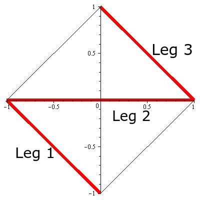
Subsection 7.3 continues the analysis of endpoints and period asymptotics begun in the previous section and introduces one of our key tools, the y and z “costs”. See equations (35). These are the differences of two periods associated to the competing geodesics coming from the Diamond, and can be thought of as ‘renormalized’ periods. We note that as the endpoints tend to infinity on our base geodesic, the coefficients $a,b$ encoding the competing geodesics must tend to a “Z” - the union of three line segments -contained in the Diamond. We denote these segments by ‘Leg 1’, ‘Leg 2’ and ‘Leg 3’. See figure 4. In this way we reduce the work to that of understanding the asymptotics of the y and z costs as we approach these three legs. We end the subsection with the statement of Proposition 7.1, a proposition on this asymptotics which almost immediately yields the Theorem.

Subsections 7.4 and 7.5 are devoted to eliminating the three Legs of the Z one at a time - thus showing that the competing geodesics cannot be simultaneously shorter than the base geodesic and share its endpoints. The method of elimination is essentially calculus, through the computing the asymptotics and the variations of the y and costs. In the short final subsection 7.6 we show how Proposition 7.1 implies the Theorem.

7.2. Set up for the proof

Recall (definition 2.3) that a seagull potential is even, achieves its global maximum value of $1$ at $x=\pm a$ and satisfies $0<F(x)<1$ for $-a<x<a$ . Moreover $F^{\prime}(x)<0$ for $x>a$ so that $F$ tends to $-\infty$ as $x\to\infty$ . It follows that $F$ ’s Hill intervals are $[-\beta,a],[-a,a],[a,\beta]$ where $x=\beta$ is the unique positive $x$ having $F(x)=-1$ . Use a scaling symmetry $x\mapsto hx$ to scale our seagull potential $F$ in order to place the maximum points $x=\pm a$ at $\pm 1$ .

Our claimed globally minimizing geodesic - is the direct heteroclinic geodesic $\gamma_{0}:\mathbb{R}\to J^{k}$ for $F$ with Hill interval $[-1,1]$ and whose $x$ curve is monotonic increasing. Thus its $x$ -curve limits to $-1$ in backward time and to $x=+1$ in forward time. Let $c_{0}=\pi_{F}\circ\gamma_{0}:\mathbb{R}\to\mathbb{R}^{3}_{F}$ be its projection to the plane -the curve referred to as the ‘base geodesic’ above. It suffices to show that $c_{0}$ is a globally minimizing in $\mathbb{R}^{3}_{F}$ to conclude Theorem B.

Next, we assume that $\beta=\sqrt{3}$ , which is to say $F(\sqrt{3})=-1$ . It follows that the other Hill intervals for $F$ are $[1,\sqrt{3}]$ and $[-\sqrt{3},-1]$ . It follows from Proposition 5.1 and the discussion around it that we have a smooth solution to the Hamilton-Jacobi equation for $F$ on the slab domain

\Omega:=\{(x,y,z):-\sqrt{3}<x<\sqrt{3}\}.

It follows from Proposition 5.1 that $c_{0}$ globally minimizes within $\Omega$ .

We now argue by contradiction. If $c_{0}$ fails to globally minimize, then there exist a family of shorter geodesics in $\mathbb{R}^{3}_{F}$ connecting distant endpoints of $c_{0}$ . Due to the Hamilton-Jacobi result just discussed, these shorter geodesics must all leave $\Omega$ . The proof will be completed by showing that these shorter geodesics cannot exist.

To begin, we argue that these shorter geodesics must be arcs of periodic geodesics. To this purpose, and to simplify book-keeping, we shift the time origin and translate as needed so that $c(0)=(0,0,0)$ . Write

c_{0}(t)=(x_{0}(t),y_{0}(t),z_{0}(t)).

It follows from the evenness of $F(x)$ that $c_{0}(-t)=(-x_{0}(t),-y_{0}(t),-z_{0}(t))$ . Since $c_{0}$ fails to globally minimize, we have, for all $T/2$ sufficiently large, a shorter geodesic $c=c_{T}$ in $\mathbb{R}^{3}_{F}$ joining $c_{0}(-T/2)$ to $c_{0}(T/2)$ .

Set

\delta=x_{0}(T/2),

so that for $T$ large $\delta$ is very close to $1$ . $T$ and $\delta$ are related, through the $x$ -differential equation, by:

(30)

T=2\int_{0}^{\delta}\frac{dx}{\sqrt{1-F(x)^{2}}}.

The allegedly shorter geodesics $c=c_{T}=(x(t),y(t),z(t))$ , being a geodesic on $\mathbb{R}^{3}_{F}$ is associated to some polynomial $G(x)=a+bF(x)$ in the pencil of $F$ . Since endpoints of $c$ and $c_{0}([-T/2,T/2])$ match up, the geodesic $c$ starts at $x=-\delta=x_{0}(-T/2)$ close to $-1$ , crosses $x=0$ and ends up at $x=\delta$ close to $+1$ , while in doing so it must leave the slab. Thus its $x(t)$ must reach a maximum point $u\geq\sqrt{3}$ , or minimum point $u<-\sqrt{3}$ and return to $x_{0}(T/2)=\delta<1$ . It follows that $x(t)$ when extended to $t\in\mathbb{R}$ is periodic, with Hill interval $[-u,u]$ , $u\geq\sqrt{3}$ . In more detail: since $x(t)$ returns from $u$ we have $G^{\prime}(u)\neq 0$ . By evenness of $G(x)$ and the fact that $x(t)$ crosses zero, the Hill interval associated to $c$ is $[-u,u]$ . In particular, since both $1$ and $\sqrt{3}$ must be in the Hill interval of $x(t)$ and since $F(1)=1,F(\sqrt{3})=-1$ , by evaluating $G$ at these two points we have that $|a+b|<1$ and $|a-b|\leq 1$ . The latter is an inequality since $u=\sqrt{3}$ is allowed, while the former is strict since $1$ must be in the interior of the Hill interval of $G$ in order for the $x$ -curve to make it all the way to $\sqrt{3}$ . We will denote the region that we just describe in the following way,

(31)

DIAM:=\{(a,b):|a+b|<1\text{ and }|a-b|\leq 1,b\neq 0\}.

DIAM is short for “diamond”. We call $DIAM_{+}$ and $DIAM_{-}$ to the point $(a,b)$ in $DIAM$ such that $0<b$ and $b<0$ , respectively. See figure 4.

We just argued that we need only compare $c_{0}$ to those geodesics arising from $G=a+bF(x)$ with $(a,b)$ lying in $DIAM$ in the $a-b$ plane. Let us formalize the above discusion by:

Definition 7.1.

[The family of competing geodesics] For each point $(a,b)$ in the square $DIAM$ and each $T>0$ let $c=c_{a,b;T}:[0,L(a,b)/2]\to\mathbb{R}^{3}_{F}$ be the geodesic arc for $G(x)=a+bF(x)$ which starts at $t=0$ at the point $c(0)=c_{0}(-T/2)$ so that $x(0)=-\delta$ , and has $\dot{x}>0$ , followed for half of its $x$ -period, $\Delta t(a,b)=L(a,b)/2$ . In this way its $x$ curve achieves a maximum of $u=u(a,b)\geq\sqrt{3}$ and ends when $x=\delta=+x_{0}(T/2)$ at time

\Delta t(a,b):=L(a,b)/2.

Remarks. 1. We do not have to worry about $x$ -periodic curves which hit both $u$ and $-u$ since these are longer than their half-period $L/2$ and hence do not minimize by (i) of Proposition 6.1.

2. If, in the definition, we took $\dot{x}<0$ at time $t=0$ instead, we would end up with the other $G$ -geodesic, again for a half-period $L/2$ . See again the arguments around (i) of Proposition 6.1 or figure 3. This other curve has the same endpoints and same length as our curve, so is identical for all our purposes. The choice $\dot{x}>0$ is just made so as to simplify the exposition.

7.3. Period asymptotics, continued

For our competing geodesics $c$ , as described in definition 7.1, the $x$ -values of both endpoints match the $x$ -values of $c_{0}$ by design. We will complete the proof of the Theorem by showing that if their y and z values match $c_{0}$ ’s then $c$ is longer: $T<L(a,b)/2$ .

To this purpose recall the half-period relations for such periodic geodesics, equations (25) and (27) for how $y$ and $z$ change in a half-period, these assert that

c(\Delta t(a,b))=(+\delta,-y_{0}(T/2),-z_{0}(T/2))+(0,\Delta y(a,b),\Delta z(a,b).

The requirement that the far endpoint of $c=c_{a,b,T}$ agrees with endpoint of $c_{0}([-T/2,T/2])$ is the requirement that their y and z periods $\Delta y(a,b),\Delta z(a,b)$ as given by (27) satisfy

(32)		$\displaystyle\Delta y(a,b)$	$\displaystyle=$	$\displaystyle\Delta y_{0}(T),$
(33)		$\displaystyle\Delta z(a,b)$	$\displaystyle=$	$\displaystyle\Delta z_{0}(T),$

where

	$\displaystyle\Delta y_{0}(T)$	$\displaystyle=$	$\displaystyle 2\int_{0}^{\delta}\frac{F(x)}{\sqrt{1-F(x)^{2}}}dx,$
	$\displaystyle\Delta z_{0}(T)$	$\displaystyle=$	$\displaystyle 2\int_{0}^{\delta}\frac{F(x)^{2}}{\sqrt{1-F(x)^{2}}}dx,$

are the corresponding changes in $y$ and $z$ suffered as we travel our heteroclinic orbit from $c_{0}(-T/2)$ to $c_{0}(T/2)$ , namely $\Delta y_{0}(T)=2y_{0}(T/2)$ and $\Delta z_{0}(T)=2z_{0}(T/2)$ ).

Remark. $\Delta y(a,b)$ and $\Delta z(a,b)$ are independent of the starting point on the curve $c$ . Compare equation (25). This $T$ -independence simplifies arguments in an essential way and is where we use the assumption that $F$ is even.

As $T\to\infty$ we have $\delta(T)\to 1$ and $\Delta y_{0}(T),\Delta z_{0}(T)\to+\infty$ . Thus, in requiring the endpoint conditions, equations (33), to hold for our competing curves we are forced to investigate the periods $\Delta y(a,b),\Delta z(a,b)$ as they tend to infinity. All three periods $\Delta t,\Delta y,\Delta z$ are analytic functions of $(a,b)\in DIAM$ away from where they blow up. Analysis of the (a,b) periods near the blow-up loci of equations (25) and (27) is the whole game now.

These periods blow up along three line segments in the diamond and nowhere else. These segments form a tilted “Z” whose middle segment, labelled $Leg2$ , is the segment of the $a$ -axis inside the diamond, see figure 4. The other two strokes of the $Z$ are made up of the bounding edges of the diamond, denoted by $Leg1$ , the locus $a+b=-1$ and $Leg3$ , the locus $a+b=+1$ . Blow up of periods along $Leg2$ , ( $b=0$ ), occurs since the Hill endpoint $u(a,b)\to\infty$ as $b\to 0$ . Blow up along $Leg1$ and $Leg3$ occur because as we approach either of these legs we have that $G(1)^{2}\to 1$ , that is, the ‘mountain peaks” $x=\pm 1$ of $G(x)^{2}$ get closer and closer to satisfying $G(x)^{2}=1$ , finally touching $G(x)^{2}=1$ at points of these legs, making periods very long through the reciprocal $1/\sqrt{1-G(x)^{2}}$ occuring in all three period integrals.

Remark. We cannot get the other critical point $x=0$ of $G(x)$ to attain the level $G(x)^{2}=1$ in the closure of the diamond and thereby lead to divergent periods, except possibly at the points $(\pm 1,0)$ which will be dealt with directly. Indeed since $|F(0)|<1$ the condition $G(0)^{2}=1$ which is $(a+bF(0))^{2}=1$ together with $|a\pm b|\leq 1$ yields $a=\pm 1$ .

We focus on the differences in periods

(34)		$\displaystyle Cost_{y}(a,b)$	$\displaystyle=$	$\displaystyle\Delta t(a,b)-\Delta y(a,b),$
(35)		$\displaystyle Cost_{z}(a,b)$	$\displaystyle=$	$\displaystyle\Delta t(a,b)-\Delta z(a,b),$

rather than the periods themselves. The advantage gained is that these difference of periods have finite limits as we tend to $Leg1$ and $Leg3$ (except for $(\pm 1,0)$ ) and so extend to continuous functions on the closure of the entire Diamond minus $Leg2$ i.e. minus the $a$ -axis. We will compare these ‘renormalized’ periods to the analogous quantities for the heteroclinic geodesic :

	$\displaystyle Cost_{0,y}(T)$	$\displaystyle=$	$\displaystyle T-\Delta y_{0}(T)$
		$\displaystyle=$	$\displaystyle 2\int_{0}^{\delta}\frac{(1-F(x))}{\sqrt{1-F(x)^{2}}}dx,$

and

	$\displaystyle Cost_{0,z}(T)$	$\displaystyle=$	$\displaystyle T-\Delta z_{0}(T)$
		$\displaystyle=$	$\displaystyle 2\int_{0}^{\delta}\frac{(1-F^{2}(x))}{\sqrt{1-F(x)^{2}}}dx,$

which both have finite limits as $T\to\infty$ , that is to say as $\delta\to 1$ .

Lemma 7.1.

The functions $Cost_{0,y}(T),Cost_{0,z}(T)$ are strictly monotone increasing in $T$ and tend to finite positive limits as $T\to\infty$ :

Cost_{0,y}(\infty)=\lim_{T\to\infty}Cost_{0,y}(T),

and

Cost_{0,z}(\infty)=\lim_{T\to\infty}Cost_{0,z}(T).

These limits can be obtained by setting $\delta=1$ in the integral expressions given just above for $Cost_{0,y}(T)$ and $Cost_{0,z}(T)$

Proof. The integrands are all positive and behave like $\sqrt{|1-x|}$ near $x=1$ .

The proof of Theorem B will be completed upon establishing the following result:

Proposition 7.1.

a) In $DIAM_{+}$ , including all along $Leg3$ we have

Cost_{y}(a,b)>Cost_{0,y}(\infty).

b) $Cost_{z}(a,b)\to+\infty$ as we approach any point of either $Leg1$ or $Leg2$ along curves in $DIAM_{-}$ , including the point $(1,0)$ .

7.4. Getting rid $Leg1$ and $Leg2$

We will prove proposition 7.1 by obtaining detailed asymptotics for the costs (periods) close to the Z. We will split the proof into two main parts, according to the two parts of the proposition. Part (b) for points in $DIAM_{-}$ itself splits into three cases, labelled below as “getting rid of points near $Leg1$ ”, “getting rid of points near $(a,b)=(1,0)$ with $b<0$ ” and ”getting rid of points near $Leg2$ with $b<0$ ”. Part (a) for $DIAM_{+}$ is presented as a single case “getting rid of points on $Leg3$ ” whose proof consists of two steps.

7.4.1. Getting rid of points near $Leg1$

On and near $Leg1$ we have $a,b<0$ . Since $b<0$ the absolute minimum of $G=a+bF(x)$ occurs when $x=1$ and its value there is $a+b$ which is $-1$ at points of $Leg1$ . The integral computing $\Delta y(a,b)$ is that of $G(x)/\sqrt{1-G(x)^{2}}$ over $[0,u]$ where $u=u(a,b)$ is the first positive solution to $G(x)=1$ . The denominator $\sqrt{1-G(x)^{2}}$ goes to zero at $x=1$ and at $x=u$ . Its behaviour near $x=u$ is like $1/\sqrt{|u-x|}$ which is integrable. Its behaviour near $x=1$ is like $-1/|1-x|$ so the integral l diverges logarithmically to $-\infty$ . It follows that as $(a,b)$ tends to any point of $Leg1$ . we have that $\Delta y(a,b)\to-\infty$ . It follows that for all $(a,b)$ sufficiently close to $Leg1$ we have $\Delta y<0$ . On the other hand, $\Delta y_{0}(T)\to+\infty$ with $T$ , the divergence being due to the behaviour of the integrand near $x=1$ . This makes it impossible to satisfy the endpoint conditions (33.)

We have not yet proved claim (a) of the proposition. Note that $\Delta t>0$ , so by our just established asymptotics for $\Delta y$ we have that $Cost_{y}\to+\infty$ as we approach $Leg1$ , while in comparisont $Cost_{0,y}(\infty)$ is finite.

Regarding the claimed behaviour of $Cost_{z}(a,b)$ near $Leg1$ in the proposition, use that $F(1)=+1$ so that an identical analysis applied to the integral expression for $\Delta z(a,b)$ shows that $\Delta z(a,b)\to-\infty$ as $(a,b)$ tends to any point of $Leg1$ . On the other hand $\Delta t(a,b)>0$ so that again $Cost_{z}(a,b)=\Delta t(a,b)-\Delta z(a,b)\to+\infty$ .

7.4.2. Getting rid of points near $(1,0)$ with $b<0$

We begin by parameterizing the lower diamond by using lines along which the upper bound $u$ of integration is constant. Since $b<0$ we have that $G$ rises from its global minimum of $a+b<1$ which occurs at $x=1$ , up past the value $a-b$ at $x=\sqrt{3}$ , and on until it hits the unique positive $u$ such that $G(u)=1$ . Set $a=1-\tau$ . Then the equation $G(u)=1$ says $(1-\tau)+bF(u)=1$ which is to say $b=\tau/F(u)$ . We then parameterize the points of $DIAM_{-}$ by

a=1-\tau,

b=\tau/F(u),u>\sqrt{3}.

In this parameterization, by fixing $u$ and varying $\tau>0$ down to $0$ we approach $(1,0)$ along lines through $(1,0)$ having slope $1/|F(u)|$ . Note as $u$ increases from $\sqrt{3}$ to $u=\infty$ the slope of these lines goes from $1$ to $0$ , thus sweeping out all of $DIAM_{-}$ .

In these coordinates

G=(1-\tau)+\frac{\tau}{F(u)}F(x),

we compute that

1-FG=1-F+\tau F-\frac{\tau}{F(u)}F(x)^{2},

which tends to $1-F$ as $\tau\to 0$ .

On the other hand, $1-G^{2}=(1-G)(1+G)$ and $1+G\leq 2$ on $[0,u]$ so that

(1-G^{2})\leq 2(1-G),

on this interval. Now observe that for $x\in[0,u]$ we have

(36)

\begin{split}1-G&=\tau-\frac{\tau}{F(u)}F(x)\\ &=\frac{\tau}{|F(u)|}(F(x)-F(u)),\end{split}

where we have used that $F(u)<0$ . Note that this expression is positive in $[0,u]$ since $F(x)>F(u)$ for $0<x<u$ . Thus for $x\in[0,u]$ we have

(1-G(x)^{2})\leq 2\frac{\tau}{|F(u)|}(F(x)-F(u)),

and hence that

\frac{1}{\sqrt{1-G(x)^{2}}}\geq\frac{|F(u)|^{1/2}}{\sqrt{2\tau}}\frac{1}{\sqrt{F(x)-F(u)}}.

Our integrand for $Cost_{z}(a,b)$ is $\frac{1-FG}{\sqrt{1-G(x)^{2}}}$ . Since $(1-F(x))\geq 0$ everywhere, our expansion of $(1-FG)$ above yields

\frac{1-F(x)G(x)}{\sqrt{1-G(x)^{2}}}\geq\{(1-F)-\tau|F(x)|+\frac{\tau}{|F(u)|}F(x)^{2}\}\frac{1}{\sqrt{2\tau}}\frac{|F(u)|^{1/2}}{\sqrt{F(x)-F(u)}}.

The three terms on the right hand side that we get by freezing $\tau$ and $u$ , namely $(1-F(x))/{\sqrt{F(x)-F(u)}}$ , $|F(x)|/{\sqrt{F(x)-F(u)}}$ and $F(x)^{2}/{\sqrt{F(x)-F(u)}}$ all have finite integrals over $[0,u]$ . After integration, let $\tau$ vary down to zero, for frozen $u$ . The last two terms go to zero like $\sqrt{\tau}$ . The first term goes to $+\infty$ like $1/\sqrt{\tau}$ .

We have shown that approaching $(1,0)$ along any line in $DIAM_{-}$ the value of $Cost_{z}(a,b)$ approaches $+\infty$ .

7.4.3. Getting rid of points near $Leg2$ with $b<0$

We will show that $\Delta z(a,-\epsilon)\to-\infty$ as $\epsilon\to 0$ with $\epsilon>0$ , and for all $a$ with $-1<a<1$ .

We start with the case $a>0,b=-\epsilon$ with $\epsilon>0$ going to zero. Since $F\leq 1$ we have that

G(x)=a-\epsilon F(x)\geq a-\epsilon,

and in particular, for $\epsilon$ small enough $G>0$ . It follows that $G(x)F(x)$ has the same sign as $F(x)$ . Let $z_{0}$ be the first positive zero of $F(x)$ so that $GF\geq 0$ on $[0,z_{0}]$ while $G(x)F(x)<0$ on $(z_{0},u]$ where $u$ is the first positive solution to $G(x)=+1$ . (Note $1<z_{0}<\sqrt{3}$ .) Then

(37)

\begin{split}\Delta z(a,-\epsilon)&=2\int_{0}^{z_{0}}\frac{G(x)F(x)}{\sqrt{1-G(x)^{2}}}dx+2\int_{z_{0}}^{u}\frac{G(x)F(x)}{\sqrt{1-G(x)^{2}}}dx\\ &=I_{0}(\epsilon)+I_{1}(\epsilon).\end{split}

The first integral $I_{0}(\epsilon)$ is positive and the second is negative. As $\epsilon\to 0$ the first integral tends to a finite positive value. Indeed on $[0,z_{0}]$ we have $a-\epsilon\leq G(x)\leq a$ so that as $\epsilon\to 0$ we have $GF/\sqrt{1-G(x)}\to aF/\sqrt{1-a^{2}}$ which is a (bounded!) polynomial on $[0,z_{0}]$ , leading to a finite limit for $I_{0}(\epsilon)$ .

Now

I_{1}(\epsilon)=-2\int_{z_{0}}^{u}\frac{G(x)|F(x)|}{\sqrt{1-G(x)^{2}}}dx,

and $G(x)$ is monotonically increasing from $a$ to $1$ on $[z_{0},u]$ so that $G\geq a$ while $1/\sqrt{1-G^{2}}\geq 1/\sqrt{1-a^{2}}$ , so

\frac{G(x)}{\sqrt{1-G(x)^{2}}}\geq\frac{a}{\sqrt{1-a^{2}}}\;\;\text{and}\;\;\frac{G(x)|F(x)|}{\sqrt{1-G(x)^{2}}}\geq\frac{a|F(x)|}{\sqrt{1-a^{2}}}

on this interval. Now we will need estimate (38) below for the Hill endpoint $u=u(a,-\epsilon)$ . We obtain the estimate by approximately solving $a-\epsilon F(x)=1$ or

-F(u)=(1-a)/\epsilon.

Since $\epsilon$ is very small we are solving a polynomial equation $p(x)=w$ for $w=(1-a)/\epsilon>>1$ , where our polynomial $p(x)$ is $-F(x)$ which has the form $p(x)=a_{0}x^{2k}+\ldots$ and in particular has degree $2k$ with $a_{0}>0$ . The solution can be expanded as

(38)

u(a,-\epsilon)=(\frac{1-a}{a_{0}})^{1/2k}\frac{1}{\epsilon^{1/2k}}+c+O(\epsilon^{1/2k}),

valid as $\epsilon\to 0$ . Here $c$ is constant. See Appendix B for this standard result regarding asymptotically solving real polynomials. Moreover we have that $|F(x)|>Ax^{2k}$ for some $A>0$ (e.g. $A=a_{0}-\epsilon$ ) for all $x$ sufficiently large. Thus

I_{1}\leq-\frac{2a}{\sqrt{1-a^{2}}}\int_{z_{0}}^{u(a,-\epsilon)}Ax^{2k}dx.

The last integral yields $-Cu^{2k+1}+O(1)=-\tilde{C}\frac{1}{\epsilon^{1+1/2k}}+O(1)$ with $C,\tilde{C}$ positive constants, showing that $I_{1}(\epsilon)\to-\infty$ as $\epsilon\to 0$ .

For the case $a\leq 0,b=-\epsilon$ , we define $u_{0}=u_{0}(\epsilon)$ and $u_{1}=u_{1}(\epsilon)$ as the positive numbers where $G(u_{0})=0$ and $G(u_{1})=1$ then $G(x)$ is negative on $[0,u_{0})$ and positive on $(u_{0},u_{1}]$ . We can take $\epsilon$ small enough to have $z_{0}<u_{0}$ , where $z_{0}$ is again the positive number such that $F(z_{0})=0$ , then $F(x)G(x)$ is negative on $[0,z_{0}]$ and $[u_{0},u_{1}]$ , while, $F(x)G(x)$ is positive on $[z_{0},u_{0}]$ . We use the same method but replace the point $z_{0}$ by $u_{0}$ , that is, we split the integral into $I_{0}(\epsilon)$ and $I_{1}(\epsilon)$ , where $I_{0}$ is over $[0,u_{0}]$ and $I_{1}$ over $[u_{0},u_{1}]$ . For small enough $\epsilon$ we have that $I_{0}(\epsilon)$ is positive and $I_{1}(\epsilon)$ is negative.

We estimate $u_{1}$ and $u_{2}$ as before by approximately solving $a-\epsilon F(x)=0$ and $a-\epsilon F(x)=1$ . Again setting $-F(x)$ to $p(x)=a_{0}x^{2k}+\ldots$ with $a_{0}>0$ we find

u_{0}(\epsilon)=(\frac{-a}{a_{0}})^{1/2k}\frac{1}{\epsilon^{1/2k}}+c_{0}+O(\epsilon^{1/2k})\;\;\text{and}\;\;u_{1}(\epsilon)=(\frac{1-a}{a_{0}})^{1/2k}\frac{1}{\epsilon^{1/2k}}+c_{1}+O(\epsilon^{1/2k}).

Here $c_{0}$ and $c_{1}$ are constant. We have that $I_{0}(\epsilon)$ and $I_{1}(\epsilon)$ now go to infinity when $\epsilon$ goes to $0$ but because $\frac{-a}{a_{0}}<\frac{1-a}{a_{0}}$ , we have that $I_{1}$ dominates $I_{0}$ so their sum again goes to negative infinity.

7.5. Getting rid of $Leg3$

At this point we need to be precise regarding the class of polynomials. Here is the promised definition.

Definition 7.2.

The specific class of polynomials for the theorem are obtained by taking $a=1$ and $W(x)$ of the form

W(x)=\frac{1}{6}(1+P(x)+(\frac{x}{\sqrt{3}})^{14})

in the equation (8) defining $F(x)$ . We insist that $P(x)$ has degree at most $14$ , $P(\sqrt{3})=1$ and

•

i) $(\frac{x}{\sqrt{3}})^{14}\leq|P(x)|\leq 1$ if $|x|\leq\sqrt{3}$ ,
•

ii) $1\leq P(x)\leq(\frac{x}{\sqrt{3}})^{14}$ if $\sqrt{3}\leq|x|$ ,
•

iii) $|P^{\prime}(x)|<\frac{14}{\sqrt{3}}|(\frac{x}{\sqrt{3}})^{13}|$ if $\sqrt{3}\leq|x|$ .

All such $F$ ’s have Hill region $[-\sqrt{3},\sqrt{3}]$ the union of the three Hill intervals $[-\sqrt{3},-1],[-1,1],[1,\sqrt{3}]$ . Moreover $F(x)<-1$ for $|x|>\sqrt{3}$ and $F(x)\to-\infty$ as $x\to\infty$ .

We establish inequality (a) of proposition 7.1 in two steps.

STEP 1. We show that $Cost_{y}$ decreases monotonically along line segments in $Diam_{+}$ connecting $(-1,0)$ to points of $Leg3$ , decreasing in the direction of $Leg3$ . See figure 5 for this picture.

STEP 2. We show, with the help of numerics, that the absolute minimum of $Cost_{y}$ restricted to $Leg3$ occurs in the interior of the $Leg$ and is larger than $Cost_{0,y}(\infty)$ .

The line segment family. As in the argument previously used to get rid of points near $(1,0)$ in $DIAM_{-}$ , these lines are determined by the condition that the far bound of integration $u$ (now characterized by $G(u)=-1$ since $b>0$ ) is constant along each line. Parameterize $DIAM_{+}$ by coordinates $\tau,u$ with $u>x_{*}$ and $-1<\tau\leq\frac{|F(u)|-1}{|F(u)|+1}$ according to

(39)		$\displaystyle a$	$\displaystyle=\tau$
(40)		$\displaystyle b$	$\displaystyle=\frac{\tau+1}{\|F(u)\|}.$

Freezing $u$ and varying $\tau$ defines a line segment in the diamond which lies on the line whose slope is $1/|F(u)|$ passing through $(a,b)=(-1,0)$ . This line segment parameterizes those $G=a+bF$ ’s in $DIAM_{+}$ whose Hill interval is $[-u,u]$ . See the red line in figure 5. Indeed since $G(x)=a+bF(x)$ we have that $G(u)=\tau-(\tau+1)=-1$ . When $\tau=-1$ all these lines pass through $(-1,0)$ . They each reach $Leg3$ ( $a+b=1$ ) when $\tau=\frac{|F(u)|-1}{|F(u)|+1}$ , and their various endpoints sweep out $Leg3$ as we vary $u$ , with $u\to\infty$ being the limit of the line segment to $Leg2$ ( $b=0$ ).

7.5.1. Completing Step 1

To complete step 1, we will prove that the cost function $Cost(a,b)$ is a strictly monotone decreasing function of $\tau$ relative to the $(\tau,u)$ parameterization of $DIAM_{+}$ described by equations (40). In preparation for this computation observe that

(41)

\begin{split}Cost_{y}(a,b)=&2\int_{0}^{u}\frac{1-G(x)}{\sqrt{1-G(x)^{2}}}dx\\ =&2\int_{0}^{u}\frac{\sqrt{1-G(x)}}{\sqrt{1+G(x)}}dx,\end{split}

and that, with points $(a,b)\in Diam_{+}$ parameterized by equation (40) we have

(42)

\begin{split}G(x)=&\tau+(\frac{\tau+1}{|F(u)|})F(x)\\ =&\frac{F(x)}{|F(u)|}+\frac{\tau}{|F(u)|}(|F(u)|+F(x)),\end{split}

from which it follows that

\displaystyle\frac{dG}{d\tau}

\displaystyle=

\displaystyle\frac{1}{|F(u)|}(F(x)-F(u)),

where we have used $F(u)<0$ .

In the $(u,\tau)$ representation of points in $DIAM_{+}$ , the $\tau$ -lines are lines of constant $u$ so we can differentiate $Cost_{y}$ with respect to $\tau$ by differentiating the right hand side of equation (41) under the integral sign. We get

\frac{d}{d\tau}Cost_{y}(a(\tau,u),b(\tau,u))=2\int_{0}^{u}\frac{d}{d\tau}\frac{\sqrt{1-G(x)}}{\sqrt{1+G(x)}}dx,

where $G=a+bF(x)$ and $a=a(\tau,u),b=b(\tau,u)$ are given by equations (40). Now then, the derivative of the integrand with respect to $\tau$ is

	$\displaystyle\frac{d}{d\tau}\frac{\sqrt{1-G(x)}}{\sqrt{1+G(x)}}$	$\displaystyle=$	$\displaystyle\frac{-1}{(1-G(x))^{\frac{1}{2}}(1+G(x))^{\frac{3}{2}}}\frac{dG}{d\tau}$
		$\displaystyle=$	$\displaystyle\frac{1}{\|F(u)\|}\frac{F(u)-F(x)}{(1-G(x))^{\frac{1}{2}}(1+G(x))^{\frac{3}{2}}}<0,$

the last inequality, the ‘ $<0$ ’, holds on the open interval $(0,u)$ as a result of the fact that $F(u)<F(x)$ for $0<x<u$ . It follows that the derivative of $Cost_{y}$ with respect to $\tau$ is strictly negative.

7.5.2. Completing Step 2

$Cost_{y}$ extends continuously to $Leg3$ , the red line segment in figure 5. This extension is given by the same integral representation (41) for $Cost_{y}$ , with the upper bound of integration $u(a,b)$ being the positive solution to $a+bF(x)=-1$ . What makes these $G$ ’s corresponding to boundary points $a+b=1$ on $Leg3$ qualitatively different than those $G$ ’s for $(a,b)$ in the interior of the diamond is that the $G$ ’s for points on $Leg3$ satisfy $G(1)=1$ so have three Hill regions: $[-1,1]$ , $[-u,1]$ and $[1,u]$ with $[-1,1]$ heteroclinic and the other two homoclinic. Parameterize $Leg3$ by $a=\mu,b=1-\mu$ , for $0<\mu<1$ . Denote the continuous extension of $Cost_{y}$ to $Leg3$ as ‘ $Cost_{bdry}$ ’. It forms a continuous function of $\mu$ , $1\leq\mu<0$ upon setting $a=\mu$ and $b=1-\mu$ and is given by

Cost_{bdry}(\mu):=2\int_{0}^{u(\mu,1-\mu)}\frac{\sqrt{1-G_{\mu}(x)}}{\sqrt{1+G_{\mu}(x)}}dx,

(43)

G_{\mu}(x):=\mu+(1-\mu)F(x).

Because of the nature of the Hill intervals of these $G_{\mu}$ ’s the integral for $Cost_{bdry}(\mu)$ incorporates the contributions of two critical geodesics for $G_{\mu}$ , one being heteroclinic with interval $[-1,1]$ and the other being homoclinic with interval $1\leq x\leq u:=u(\mu,1-\mu)$ . Consequently we can write

Cost_{bdry}(\mu):=Cost_{heter}(\mu)+Cost_{homoc}(\mu),0<\mu<1,

where the first integral goes from $0$ to $1$ and the second from $1$ to $u(\mu,1-\mu)$ . If we take the limit $\mu\to 0$ corresponding to $G_{0}(x)=F(x)$ , then $u\to\sqrt{3}$ from above and we find that

\lim_{\mu\to 0}Cost_{bdry}(\mu)=Cost_{0,y}(\infty)+Cost_{homoc}(\infty).

The last term $Cost_{homoc}(\infty)$ is the integral from $1$ to $\sqrt{3}$ of the integrand of equation (41 ) except with $G$ replaced by $F$ . Expressed this way this last term is clearly positive. It is this last positive jump of $Cost_{homoc}(\infty)$ which gives us our big advantage along $Leg3$ , making the completion of the proof possible.

To finish the proof, we need to prove the following inequalities:

a) $Cost_{0,y}(\infty)<0.58$ .

b) $0.58<Cost_{bdry}(\mu)$ for all $\mu$ with $0<\mu<1$ .

To prove these inequalities we introduce auxilary functions

\begin{split}F_{0}(x)&:=1-\frac{(x^{2}-1)^{2}}{6}(1+2(\frac{x}{\sqrt{3}})^{14}),\\ F_{1}(x)&:=1-\frac{(x^{2}-1)^{2}}{6}(2+(\frac{x}{\sqrt{3}})^{14}).\\ \end{split}

$F_{0}(x)$ corresponds to $P(x)=(\frac{x}{\sqrt{3}})^{14}$ while $F_{1}(x)$ corresponds to $P(x)=1$ in definition 7.2 specifying the class of polynomials, the definition immediately following the statement of theorem B.

a) Since $(\frac{x}{\sqrt{3}})^{14}\leq P(x)\leq 1$ if $|x|<\sqrt{3}$ according to definition 7.2 we have that

(44)

F_{1}(x)\leq F(x)\leq F_{0}(x),\text{ for }|x|\leq\sqrt{3}.

The function $f\mapsto\sqrt{\frac{1-f}{1+f}}$ is strictly monotone decreasing on the interval $[-\sqrt{3},\sqrt{3}]$ from which it follows that

\sqrt{\frac{1-F_{0}(x)}{1+F_{0}(x)}}\leq\sqrt{\frac{1-F(x)}{1+F(x)}}\leq\sqrt{\frac{1-F_{1}(x)}{1+F_{1}(x)}},x\in[\sqrt{3},\sqrt{3}].

Using the upper bound for $x\in[-1,1]$ we get

Cost_{0,y}(\infty)=2\int_{0}^{1}\sqrt{\frac{1-F(x)}{1+F(x)}}dx\leq 2\int_{0}^{1}\sqrt{\frac{1-F_{1}(x)}{1+F_{1}(x)}}dx.

A numerical integration yields

2\int_{0}^{1}\sqrt{\frac{1-F_{1}(x)}{1+F_{1}(x)}}dx=0.5790109314,

establishing (a).

b) Since $1\leq P(x)\leq(\frac{x}{\sqrt{3}})^{14}$ if $\sqrt{3}<|x|$ according to the specifications of definition 7.2 we have

(45)

F_{0}(x)\leq F(x)\leq F_{1}(x),\text{ for }\sqrt{3}\leq|x|\leq\infty.

We consider the family $G_{\mu}$ as in equation (43). Its Hill region has the form $[-u(\mu),u(\mu)]$ where $\sqrt{3}\leq u(\mu)$ , $\mu\to u(\mu)$ is an invertible function. (As before the slope of the line joining $(-1,0)$ to $(\mu,1-\mu)$ on $Leg3$ is proportional to $1/|F(u)|$ .) We find $\mu(u)$ by solving $G_{\mu(u)}(u)=-1$ . We get $\mu(u)=\frac{-1-F(u)}{1-F(u)}$ . Plug $\mu(u)$ in $G_{\mu(u)}(x)$ and after a simplification we find

Cost_{bdry}(u)=2\int_{0}^{u}\sqrt{\frac{1-F(x)}{F(x)-F(u)}}dx.

Set

Lowbound(u)=2\int_{0}^{\sqrt{3}}\sqrt{\frac{1-F_{0}(x)}{F_{0}(x)-F_{0}(u)}}dx+2\int_{\sqrt{3}}^{u}\sqrt{\frac{1-F_{1}(x)}{F_{0}(x)-F_{0}(u)}}dx.

We claim that

Lowbound(u)<Cost_{bdry}(u).

Indeed $1-F_{0}(x)<1-F(x)$ on $[0,\sqrt{3}]$ and $1-F_{1}(x)<1-F(x)$ on $[\sqrt{3},u]$ by inequality (45). And ${\frac{1}{F_{0}(x)-F_{0}(u)}}<\frac{1}{F(x)-F(u)}$ on the entire interval $[0,u]$ . This last inequality holds because

\begin{split}F(x)-F(u)&\leq F_{0}(x)-F_{0}(u),\text{ for }0\leq x\leq u.\\ \end{split}

which in turn is true since it is equivalent to

\begin{split}(x^{2}-1)^{2}((\frac{x}{\sqrt{3}})^{14}-P(x))&\leq(u^{2}-1)^{2}((\frac{u}{\sqrt{3}})^{14}-P(u)),\text{ for }0\leq x\leq u,\end{split}

which is seen to hold upon using the properties of 7.2. Indeed, according to these properties $1\leq P(u)\leq(\frac{u}{\sqrt{3}})^{14}$ since $u>\sqrt{3}$ , so the right side of the inequality is positive. For $\sqrt{3}<x<u$ the left hand side is monotone increasing, reaching a maximum when $x=u$ and the inequality becomes equality. For $0<x<\sqrt{3}$ the left hand side of the inequality is negative, again by one of the properties of 7.2.

Using Maple’s built-in numerical integrator, we performed these integrals defining $Lowbound(u)$ to a tolerance of $10^{-10}$ and plotted the results. See figure 6 for a plot of the function $Lowbound(u)-.58$ versus $u$ for $u\geq\sqrt{3}$ . The plot shows the function is positive and convex yielding that $0.58<Lowbound(u)$ . (One can verify directly that $Lowbound(u)\to\infty$ as $u\to\infty$ .) See also figure 7.

Now we are ready to finish the proof of proposition 7.1.

7.5.3. Proof of proposition 7.1

Proof.

Inequality (a) of proposition 7.1 follows immediately from the lemma. To repeat the argument: Move from any interior $(a,b)$ point to the boundary by moving along a $\tau$ -line until you hit a point on $Leg3$ . Since $Cost_{y}$ decreases monotonically along the $\tau$ -lines the value limited to on $Leg3$ , whatever it be, is less than its original value. Once on $Leg3$ , $Cost_{y}$ is greater than $Cost_{0}(\infty)$ . ∎

7.6. Proof theorem B

Proof.

We show how proposition 7.1 completes the proof of Theorem B. All points of $DIAM_{+}$ are excluded by (a) of the proposition and the following logic. If a competing geodesic coming from $DIAM_{+}$ shares endpoints with $c_{0}$ for some $T$ then it shares y-endpoint values: $\Delta y_{0}(T)=\Delta y(a,b)$ . By (a), $Cost_{y}(a,b)>Cost_{0,y}(\infty)$ . By lemma 7.1 $Cost_{0,y}(\infty)>Cost_{0,y}(T)$ , so that $\Delta t(a,b)-\Delta y(a,b)>T-\Delta y_{0}(T)$ . Thus $\Delta t(a,b)>T$ : the competing geodesic is longer.

All competing geodesics coming from points of $DIAM_{-}$ are excluded using (b) of the proposition and a similar logic. Since the endpoint conditions (equations(33)) must hold for all sufficiently large $T$ and since $\Delta z_{0}(T),\Delta y_{0}(T)\to\infty$ with $T$ we can restrict ourselves to $(a,b)$ in an arbitrarily small neighborhood of $Leg1$ or $Leg2$ , since only here in $DIAM_{-}$ do the (a,b) periods blow up. But then $Cost_{z}(a,b)\to\infty$ as we approach either leg. In particular, for $(a,b)$ close to any point on either Leg we have $Cost_{z}(a,b)>>Cost_{0,z}(\infty)>Cost_{0,z}(T)$ . Now the same logic and inequalities as in the last two sentences of the previous paragraph carry through with $y$ replaced by $z$ . ∎

Appendix A Lagrangian approach to geodesic equations.

We derive the geodesic equations on the jet space $J^{k}$ using a Lagrangian approach. We can interpret the coordinate $u_{k}$ as $\frac{d^{k}u_{0}}{dx^{k}}$ . We can do so along any arc of any horizontal curve $\gamma(t)$ in $J^{k}$ which is nowhere tangent to the vertical $X_{2}={{\partial}\over{\partial u_{k}}}$ direction. For then $\dot{x}\neq 0$ so that we can take $x$ rather that $t$ as the independent variable parameterizing the curve Any such curve is then the $k$ -jet of the function $f(x)=u_{0}(x)$ so that along the curve $u_{i}=d^{i}u_{0}/dx^{i}$ . We can rewrite the arc-length of such a horizontal curve on $J^{k}$ as follow

	$\displaystyle\int\sqrt{\dot{x}^{2}+\dot{u}_{k}^{2}}dt$	$\displaystyle=$	$\displaystyle\int(\sqrt{1+(\frac{d^{k+1}u_{0}}{dx^{k+1}})^{2}})\frac{dx}{dt}dt$
		$\displaystyle:=$	$\displaystyle\int\sqrt{1+(\frac{d^{k+1}u_{0}}{dx^{k+1}})^{2}}dx.$

The last integrand is a Lagrangian depending on higher derivatives, but is independent of $x$ . Using the Euler-Lagrange equation for higher order derivatives (see [6], pages 40-42) we have

\frac{d^{k+1}}{dx^{k+1}}(\frac{\frac{d^{k+1}u_{0}}{dx^{k+1}}}{\sqrt{1+(\frac{d^{k+1}u_{0}}{dx^{k+1}})^{2}}})=0\;\;\Longrightarrow\;\;\frac{\frac{d^{k+1}u_{0}}{dx^{k+1}}}{\sqrt{1+(\frac{d^{k+1}u_{0}}{dx^{k+1}})^{2}}}=a_{0}+a_{1}x+\dots+a_{k}x^{k}.

Define $F(x):=a_{0}+a_{1}x+\dots+a_{k}x^{k}$ to be this guaranteed polynomial. Observe that the function $\beta\mapsto f=\beta/\sqrt{1+\beta^{2}}$ is invertible with inverse $f\mapsto f/\sqrt{1-f^{2}}$ and set $f=F(x)$ , $\beta=\frac{d^{k+1}u_{0}}{dx^{k+1}}=du_{k}/dx$ to obtain

\frac{du_{k}}{dx}=\frac{d^{k+1}u_{0}}{dx^{k+1}}=\frac{F(x)}{\sqrt{1-F^{2}(x)}}.

This equation is the same as the one from proposition 4.1. See figure 8 for the relation between the various dependent variables and the angle $\theta$ made by our geodesic relative to the frame $X_{1},X_{2}$ , i.e. to $\cos(\theta)X_{1}+\sin(\theta)X_{2}=\dot{\gamma}$ . We see that $\frac{dx}{dt}=\sqrt{1-F^{2}(x)}$ and $\dot{u}_{k}=F(x)$ . Using the equations from the Pfaffian system, equation (2), (that is, what it means to locally be a k-jet) we find the rest of the geodesics equations (3).

Appendix B Multiplication on $J^{k}$ .

$J^{k}$ forms a $k+2$ -dimensional Lie group with multiplication

(x,u_{k},\dots,u_{0})\cdot(x^{\prime},u^{\prime}_{k},\dots,u^{\prime}_{0})=(x+x^{\prime},u_{k}+u^{\prime}_{k},u_{k-1}+u^{\prime}_{k-1}+u_{k}x^{\prime},\dots,u_{0}+u^{\prime}_{0}+u_{1}x^{\prime}).

The neutral element is $(0,0,\dots,0)$ and the inverse is

(x,u_{k},\dots,u_{0})^{-1}=(-x,-u_{k},-u_{k-1}+x^{\prime}u_{k},\dots,-u_{0}+xu_{1}-x^{2}u_{2}+\dots+(-1)^{k-1}u_{k}x^{k}).

One computes s t that the standard frame $\{X_{1},\dots,X_{k+2}\}$ for $J^{k}$ generated by $X_{1},X_{2}$ (equation (1)) satisfies

\begin{split}X_{1}(g)=(L_{g})_{*}(e_{1}),\;\cdots,\;X_{k+2}(g)=(L_{g})_{*}(e_{k+2}),\\ \end{split}

where $g=(x,u_{k},\dots,u_{0})$ , $(L_{g})_{*}$ is the push forward by left translation by $g$ , and $e_{i}$ is the canonical base on $\mathbb{R}^{k+2}$ . This computation exhibits the $X_{i}$ as a basis for the left-invariant vector fields on $J^{k}$ .

Appendix C Inverting polynomials near infinity

In getting rid of points $(a,b)$ near Leg 2 having $b<0$ we used an estimate for the solution to a real polynomial equation $p(x)=w$ for $w=1/\epsilon$ very large. See equation (38). Here we derive that estimate.

Write

	$\displaystyle w$	$\displaystyle=$	$\displaystyle p(x)$
		$\displaystyle=$	$\displaystyle a_{0}x^{n}+a_{1}x^{n-1}+\ldots+a_{n},$

Consider $w>>1$ and suppose $a_{0}>0$ . Write the reciprocal of both sides to get

	$\displaystyle\frac{1}{w}$	$\displaystyle=$	$\displaystyle\frac{1}{a_{0}x^{n}+a_{1}x^{n-1}+\ldots+a_{n}}$
		$\displaystyle=$	$\displaystyle\frac{1}{a_{0}x^{n}(1+b_{1}x^{-1}+\ldots+b_{n}x^{-n})},$

where $b_{i}=a_{i}/a_{0}$ . Rewrite this relation in terms of the coordinates $u=1/x,v=1/w$ about infinity in the domain and range:

v=\frac{1}{a_{0}}u^{n}[1+b_{1}u+\ldots b_{n}u^{n}]^{-1},

which we can partially invert

(a_{0}v)^{1/n}=u[1+b_{1}u+\ldots b_{n}u^{n}]^{-1/n}.

The right hand side function of $u$ is a near-identity analytic transformation near $u=0$ so is invertible. Write $f(u)$ for its inverse: $f(u)=u-\frac{1}{n}(b_{1}u)^{2}+\ldots$ by the binomial theorem. Then $u=f((a_{0}v)^{1/n})$ . Since $x=1/u$ and $w=1/v$ this gives us that $x=1/f((a_{0}/w)^{1/n})=1/[(a_{0}/w)^{1/n}-\frac{1}{n}(b_{1}(a_{0}/w)^{1/n})^{2}+\ldots]$ . Expanding out we obtain the desired:

x=\frac{w^{1/n}}{a_{0}^{1/n}}+\frac{1}{n}b_{1}+O(\frac{1}{w}).

References

[1] A.A. Ardentov, Yu. L. Sachkov, Conjugate points in Nilpotent Sub-Riemannian Problem on the Engel Group, Journal of Mathematical Sciences September 2012; DOI:10.100z/s10958-013-1584-2
[2] A.A. Ardentov, Yu. L. Sachkov, Extremal trajectories in a nilpotent sub-Riemannian problem on the Engel group, Matematicheskii Sbornik 202:1131-54; DOI10.1070/SM2011v202n11ABEH004200
[3] A.A. Ardentov, Yu. L. Sachkov, Cut time in sub-Riemannian problem on Engel group, (English summary) ESAIM Control Optim. Calc. Var. 21 (2015), no. 4, 958?988.
[4] R. Bryant and L. Hsu, Rigidity of Integral Curves of Rank Two Distributions, Invent. Math., vol 114, pp. 435–461, (1993).
[5] J. Cheeger and D. Ebin, Comparison Theorems in Riemannian Geometry, North-Holland, (1975).
[6] I.M. Gelfand and S.V. Fomin, Calculus of Variations, pp 40-42, Dover, (2000).
[7] Alfonso Anzaldo-Meneses and Felipe Monroy-Perez Goursat distribution and sub-Riemannian structures, December 2003, Journal of Mathematical Physics
[8] Alfonso Anzaldo-Meneses and Felipe Monroy-Perez, Integrability of nilpotent sub-Riemannian structures, preprint; INRIA; inria-00071749, (2003).
[9] Alfonso Anzaldo-Meneses and Felipe Monroy-Perez, Optimal Control on Nilpotent Lie Groups Journal of Dynamical and Control Systems, October 2002.
[10] L. Landau and E. Lifshitz, Mechanics, vol. 1 of a Course of Theoretical Physics, Pergamon Press, [1976].
[11] E. Hakavuori and E. Le Donne, Blowups and blowdowns of geodesics in Carnot groups, arXiv:1806.09375, [2018].
[12] R. Montgomery, A Tour of SubRiemannian Geometry, Mathematical Surveys and Monographs, vol. 91, American Math. Society, Providence, Rhode Island, 2002.
[13] R. Montgomery and M. Zhitomirskii Points and Curves in the Monster Tower, American Mathematical Soc. 2010 .
[14] Ben Warhurst, Jet spaces as nonrigid Carnot groups Journal of Lie Theory, Volume 15, 341–356, (2005)
[15] Yu. Sahkov, Homogeneous sub-Riemannian geodesic on the group of motion of the plane, Diffrential equations, 2021, Vol. 57, No. 11, pp. 1568-1572.

Geodesics in Jet Space.

Abstract.

Key words and phrases:

1. Introduction: Motivation, results, acknowledgement

1.1. Acknowledgement

2. Set-up. Background. Theorems. Overview.

2.1. Set-up and Carnot group structure.

2.2. Geodesic equations

Background Theorem.

Proposition 2.1.

Proof.

Remark 2.1.

Definition 2.1.

Definition 2.2.

2.3. Main Results

Theorem A.

Definition 2.3.

Theorem B.

2.4. Miscellany.

2.4.1. Vertical lines as abnormal geodesics.

2.4.2. Scaling.

2.4.3. The other jet submetries.

3. Proof of theorem A

3.1. Case (i) the x-periodic case

Proposition 3.1.

Proof.

Proof.

3.2. Case (ii) : the heteroclinic turn-back case.

Definition 3.1.

Lemma 3.1.

Proof.

4. Setting up for theorem B.

4.1. The intermediate Magnetic space

4.2. Magnetic geodesics.

Definition 4.1.

Lemma 4.1.

4.3. Periods I

Proposition 4.1.

Proof.

5. Calibrations: a Hamilton-Jacobi method for local minimality

Definition 5.1.

Remark 5.1.

Proposition 5.1.

Proof.

Definition 5.2.

Proposition 5.2.

Proof.

6. Magnetic cut times. Periods II.

6.1. Definitions of cut and Maxwell times.

Definition 6.1.

6.2. Cut time and xx-period

Lemma 6.1 (Maxwell point, reflection argument).

Proof.

Proposition 6.1.

Proof.

Definition 6.2.

6.3. Periods II

7. Proof of theorem B

7.1. Outline

7.2. Set up for the proof

Definition 7.1.

7.3. Period asymptotics, continued

Lemma 7.1.

Proposition 7.1.

7.4. Getting rid L​e​g​1Leg1 and L​e​g​2Leg2

7.4.1. Getting rid of points near L​e​g​1Leg1

7.4.2. Getting rid of points near (1,0)(1,0) with b<0b<0

7.4.3. Getting rid of points near L​e​g​2Leg2 with b<0b<0

7.5. Getting rid of L​e​g​3Leg3

Definition 7.2.

7.5.1. Completing Step 1

7.5.2. Completing Step 2

7.5.3. Proof of proposition 7.1

Proof.

7.6. Proof theorem B

Proof.

Appendix A Lagrangian approach to geodesic equations.

Appendix B Multiplication on JkJ^{k}.

Appendix C Inverting polynomials near infinity

References

6.2. Cut time and $x$ -period

7.4. Getting rid $Leg1$ and $Leg2$

7.4.1. Getting rid of points near $Leg1$

7.4.2. Getting rid of points near $(1,0)$ with $b<0$

7.4.3. Getting rid of points near $Leg2$ with $b<0$

7.5. Getting rid of $Leg3$

Appendix B Multiplication on $J^{k}$ .