In search of peak human athletic potential: A mathematical investigationPreprint: AIP/123-QED
Abstract
This paper applies existing and new approaches to study trends in the performance of elite athletes over time. We study both track and field scores of men and women athletes on a yearly basis from 2001 to 2019, revealing several trends and findings. First, we perform a detailed regression study to reveal the existence of an “Olympic effect”, where average performance improves during Olympic years. Next, we study the rate of change in athlete performance and fail to reject the notion that athlete scores are leveling off, at least among the top 100 annual scores. Third, we examine the relationship in performance trends among men and women’s categories of the same event, revealing striking similarity, together with some anomalous events. Finally, we analyze the geographic composition of the world’s top athletes, attempting to understand how the diversity by country and continent varies over time across events. We challenge a widely held conception of athletics, that certain events are more geographically dominated than others. Our methods and findings could be applied more generally to identify evolutionary dynamics in group performance and highlight spatio-temporal trends in group composition.
Throughout time, humans have aspired to improve in a wide range of societal aspects. Over the last several hundred years, we have seen significant advances in technology, health, the economy, education, and other fields. Further progress in such areas of human life is expected to continue in the coming years. In areas such as sports and athletics, there may be an ultimate limit to human potential. The recent completion of The Tokyo 2020 Olympic and Paralympic Games piqued our interest in studying evolutionary patterns in human athletic performance over the last two decades. Throughout this paper, we seek to better identify patterns and structural similarities in men and women’s track and field events. We seek to identify anomalous trajectories, explore the existence and potential impact of an “Olympic effect” on collective athlete performance, measure the similarity of performance trends between men and women, and study the variance in geographic representation of events’ top athletes. We hope that this work will further encourage the application of techniques from the nonlinear dynamics community to better understand time-varying behaviors in athletics, and sports more generally.
I Introduction
Every year, there are many competitions at which the world’s top athletes participate. Athletic sports comprise two main categories: track, in which athletes are scored by their times (and a lower measured time is a better result), and field, in which athletes are scored by a distance thrown or jumped (and a higher distance is a better result). Typically, competitions consist of both track and field events. In all events, elite athletes seek the marginal improvements necessary to best their opponents, where seconds, split seconds, and centimeters may make the difference. Among all competitions, the Olympic Games, held every four years, are the most well-known and prestigious, attracting competitors worldwide. The modern Olympic Games were first held in 1896 in Athens, Greece, and winning an Olympic gold medal is considered one of sport’s greatest achievements.
Given the intense competition around score improvements, athletes, commentators, analysts, and fans alike all share an interest in closely tracking the best results over time. There are numerous reasons for understanding the trends in these results, including fan interest, the identification of avenues for improvement, certain countries performing better than others, allocation of dedicated resources to burgeoning young athletes, and identifying athletes with promising growth trajectories who could become suitable brand ambassadors for various companies.
For this purpose, there has been a substantial body of statistical research on sports conducted both on a private and academic basis.Elderton and Wood 1945; Kimber and Hansford 1993; Gabel and Redner 2012; Pawlowski 2013; Wu et al. 2021 In particular, statisticians have applied extreme value theory to investigate records, namely singularly outstanding performances, in athletics.Einmahl and Magnus 2008; Robinson and Tawn 1995; Gembris, Taylor, and Suter 2002; Barão and Tawn 1999 However, there have been limited applications of nonlinear dynamics and physically-inspired mathematics to understand patterns and trends across various sports.Ribeiro, Mukherjee, and Zeng 2012; Merritt and Clauset 2014; Clauset, Kogan, and Redner 2015; Kiley et al. 2016 Our paper builds on a long literature of multivariate time series analysis, methods that are more frequently applied to other domains, including epidemiology,James, Menzies, and Bondell 2022; James and Menzies 2020; Chowell et al. 2016; James, Menzies, and Radchenko 2021; Manchein et al. 2020; Blasius 2020; James and Menzies 2021a; James and Menzies 2022a finance,Drożdż et al. 2020a; James and Menzies 2021b; Drożdż, Kwapień, and Oświęcimka 2021; James and Menzies 2021c; Drożdż et al. 2020b; James and Menzies 2021d; Wątorek et al. 2020; Prakash et al. 2022 and other fields.Vazquez 2006; Mendes and Beims 2018; Shang et al. 2020 Methods of time series analysis are broad, including parametric models, Hethcote 2000; Perc et al. 2020 distance analysis and correlation, Moeckel and Murray 1997; Székely, Rizzo, and Bakirov 2007; Mendes, da Silva, and Beims 2019; James et al. 2020 network models, Karaivanov 2020; Ge et al. 2020; Xue et al. 2020 clustering Machado and Lopes 2020 and many others. Ngonghala, Iboi, and Gumel 2020; Cavataio and Schnell 2021; Náraigh and Byrne 2020; Glass 2020 In this paper, we draw upon numerous existing techniques, including linear regression,Hastie, Tibshirani, and Friedman 2009 trajectory analysis Nguefack et al. 2020; Nagin 2014, inconsistency analysis,James, Menzies, and Chan 2021; James and Menzies 2022b agglomerative hierarchical clustering Müllner 2013 and geographic dispersion.James, Menzies, and Bondell 2021
This paper aims to study trends and relationships between the performance (and composition) of male and female athletes. First, Section III performs several regressions to investigate the existence and extent of an “Olympic effect,” in which athletes’ scores are usually (but not always) superior during Olympic years. Section IV examines the linearity of score increments more closely to investigate whether there is evidence of a recent leveling off in average scores. Subsequently, Section V takes a closer analysis of the yearly changes in scores and shows broad alignment between male and female performance in corresponding events. Next, we analyze the trajectories of performances over time and determine inconsistencies between the performance of men and women in Section VI. Finally, Section VII analyzes the composition of top athletes on an event-by-event basis. We track the extent of the geographic spread of the best athletes across the world over time. In particular, we show surprising uniformity in this variance, challenging the notion that some events are more dominated by smaller collections of countries than others.
II Data
Our data consists of the top 100 scores (times and distances, respectively) recorded each year in the men and women’s competitions of 16 track and field events. Our data source is World Athletics (https://www.worldathletics.org). Due to the cancellation of many sporting events during COVID-19 and 2021’s being incomplete, we exclude 2020 and 2021 from our analysis window. Thus, our data spans Track events are scored in times, with shorter times scoring better, while field events are scored in distances, with larger distances scoring better. Thus, we consistently analyze track and field events separately, and briefly consider the difference in behavior between the top and 100 scores in each event. Our events are the following: high jump, long jump, pole vault, triple jump, discus, hammer throw, javelin, shot put, 10 000 meters (10K), 5000 meters (5K), 3000 meters (3K), 1500 meters (1500m), 800m, 400m, 200m and 100m. All these running events are of a flat elevation. Throughout the manuscript, let be the average of the top scores in the women and men’s competition of the event indexed by .
| Comparison of linear regression models | |||||||
|---|---|---|---|---|---|---|---|
| Event | Model 1 Adj. | Model 2 Adj. | Model 3 Adj. | Top 100 | Top 100 | Top 10 | Top 10 |
| Men’s high jump | 0.24 | 0.33 | 0.26 | .0005∗∗ | .0046∗ | .0009∗∗ | .007 |
| Women’s high jump | 0.13 | 0.24 | 0.45 | -.0004∗∗ | .005∗ | -.0008∗ | .0073 |
| Men’s long jump | 0.11 | 0.16 | 0.13 | .0014∗ | .016 | .003∗ | -.01 |
| Women’s long jump | 0.26 | 0.47 | 0.61 | .003∗ | .036∗∗ | .0021 | .073∗∗ |
| Men’s pole vault | -0.03 | 0.0014 | -0.05 | .0007 | .016 | .0006 | -.004 |
| Women’s pole vault | 0.89 | 0.93 | 0.94 | 0.01∗∗∗ | 0.035∗∗ | .01∗∗∗ | .04∗∗ |
| Men’s triple jump | -0.06 | 0.13 | 0.08 | -.0002 | .066∗∗ | -.0003 | -.02 |
| Women’s triple jump | 0.06 | 0.30 | 0.34 | -.0042 | .085∗∗ | -.01∗∗ | .16∗∗∗ |
| Men’s discus | 0.27 | 0.71 | 0.68 | .039∗∗∗ | .62∗∗∗ | -.04∗ | .33 |
| Women’s discus | 0.04 | 0.52 | 0.50 | .024∗ | .75∗∗∗ | .06∗∗ | .37 |
| Men’s hammer throw | 0.54 | 0.79 | 0.84 | -.08∗∗∗ | .67∗∗∗ | -.21∗∗∗ | .4 |
| Women’s hammer throw | 0.60 | 0.71 | 0.70 | 0.19∗∗∗ | 1.16∗∗ | .23∗∗∗ | .63 |
| Men’s javelin | 0.49 | 0.51 | 0.46 | 0.09∗∗∗ | 0.33 | .05 | -.67 |
| Women’s javelin | 0.63 | 0.73 | 0.70 | 0.08∗∗∗ | 0.45∗∗ | .09∗∗∗ | .24 |
| Men’s shot put | 0.71 | 0.73 | 0.70 | 0.033∗∗∗ | 0.095 | .04∗∗∗ | -.08 |
| Women’s shot put | 0.05 | 0.24 | 0.15 | .007 | .138∗∗ | -.01∗∗ | .24∗∗∗ |
| Men’s 10K | 0.12 | 0.37 | 0.66 | -.58∗∗ | -9.9∗∗ | 0.27 | -5.8 |
| Women’s 10K | -0.05 | 0.17 | 0.29 | -.2 | -13.7∗∗ | .11 | -26.8∗∗ |
| Men’s 5K | -0.05 | 0.03 | -0.09 | 0.04 | -1.9 | .19 | -.92 |
| Women’s 5K | 0.003 | 0.16 | 0.14 | -.17 | -4.0∗ | -.46∗∗∗ | -1.3 |
| Men’s 3K | 0.50 | 0.53 | 0.57 | 0.3∗∗∗ | 1.3 | .14 | -.33 |
| Women’s 3K | -0.06 | -0.07 | 0.15 | -.0006 | 1.7 | -.16 | 4.0 |
| Men’s 1500m | 0.06 | 0.08 | 0.19 | -.023 | -.25 | .02 | .26 |
| Women’s 1500m | 0.69 | 0.70 | 0.66 | -.13∗∗∗ | -.36 | -.16∗∗∗ | .05 |
| Men’s 800m | 0.54 | 0.63 | 0.60 | -.03∗∗∗ | -.15∗∗ | -.02 | .24 |
| Women’s 800m | 0.20 | 0.58 | 0.53 | -0.02∗∗ | -0.4∗∗∗ | -.008 | -.63∗∗ |
| Men’s 400m | 0.58 | 0.55 | 0.52 | -0.2∗∗∗ | -.02 | -.03∗∗∗ | -.05 |
| Women’s 400m | 0.05 | 0.30 | 0.23 | -.008 | -.18∗∗ | -.01 | -.12 |
| Men’s 200m | 0.86 | 0.86 | 0.85 | -.014∗∗∗ | -.015 | -.01∗∗∗ | -.02 |
| Women’s 200m | 0.73 | 0.86 | 0.85 | -.016∗∗∗ | -.09∗∗∗ | -.02∗∗∗ | -.11∗∗ |
| Men’s 100m | 0.85 | 0.89 | 0.89 | -.007∗∗∗ | -.02∗∗ | -.005∗∗∗ | -.04∗ |
| Women’s 100m | 0.87 | 0.89 | 0.90 | -.009∗∗∗ | -.02∗∗ | -.009∗∗∗ | -.05∗∗ |
III Olympic effect regressions
In this section, we test the existence of an Olympic effect - a phenomenon where athletic performance is superior during Olympic years. To study this effect, we fit several linear regression models for both men and women’s events. In model 1, we assume that athletic performance is a linear function over time subject to additive white noise. For each men’s event , model 1 is formulated as follows:
| (1) |
Here, is the mean of the top scores in year , is the model’s intercept and is the trend of event performance over time, both of which we estimate in the modeling procedure. We implement this for both and 100, averaging the top 10 and 100 scores per year, respectively. As is typical in an ordinary least squares (OLS) framework, is assumed to be independently and identically distributed from a Gaussian distribution centered at zero. In Appendix A, we include some necessary validation of technical hypotheses that underpin the reliability of the linear regression model.
In model 2, we assume that athletic performance is a linear function over time and explicitly model an Olympic effect with an indicator function during Olympic years. Model 2 is formulated as
| (2) |
Here, is an indicator function taking a value of 1 only during Olympic years, so measures the extent of this effect.
Finally, model 3 explores the possibility of 4-year periodic behavior in scores not primarily driven by Olympic years. Specifically, we fit the response variable of mean scores against not only year , but also a categorical variable according to whether is 0,1,2 or 3 (modulo 4). We encode this with three dummy variables as follows:
| (3) |
Here, is an indicator function taking value 1 if (mod 4). Then and are the linear coefficients for years that are 1,2 and 3 modulo 4, respectively. As is standard with dummy encoding of categorical variables, four separate categories are encoded with three numeric indicator variables. It is arbitrary which category is not included in this encoding, so we have chosen to distinguish the coefficient of Olympic years by not including an term here. All three models are written analogously for women’s events, using as our response variable.
We fit these three models to all track and field events for both men and women and explore the insights therein. Our general approach is to find a simple model that generalizes well across most events. Accordingly, we validate our models’ estimates using adjusted , where additional parameters yield a complexity penalty. Table 1 shows the adjusted for all three models, where one can see that model 2 is generally the best candidate model. Specifically, model 2 has the best adjusted score in 58% of events.
In the final four columns of the table, we present and for model 2, in the cases where and respectively. represents the coefficient of the linear term, and represents the coefficient of the Olympic indicator function. Table 1 demonstrates that most events display an improving linear trend in performance, with a positive Olympic effect (greater distances for field events and lower times for track events). In the case where , all field events exhibit a positive term, with the majority being statistically significant, an Olympic effect where performance improves during Olympic years. Findings on the track are similar, where all but two events (the men and women’s 3000 meters) display a negative term, indicating improved track performance during Olympic years.
Interestingly, this Olympic effect appears to be less ubiquitous in the case where . Five field events (men’s long jump, men’s pole vault, men’s triple jump, men’s javelin, and men’s shot put) display a negative Olympic effect, while those that are positive are mostly not statistically significant. That is, among the top 10 athletes, we do not observe evidence that Olympic years are associated with increased average athletic performance. Similarly, with track, Olympic years provide less consistently positive boosts in performance. Four track events (men’s 800m, women’s 1500m, men’s 1500m, and women’s 3000m) have a positive (but not significant) term, again indicating less evidence for improved performance during Olympic years.


For most track and field events, especially with , model 2 does a good job of capturing the true essence of the data: a linear trend accompanied by a (generally positive) effect on average performance during Olympic years. Figure 1 shows model 2’s estimates for four events: two track events and two field events when . Figures 1(a) and 1(b), which display the men’s 100m and women’s 200m, respectively, show typical results for track events. Each features an evident linear trend of reduced times and Olympic effect of improvement during Olympic years.
Turning to the field events, Figure 1(c), displaying the women’s pole vault, shows a typical result for the field. A positive linear term is evident, highlighting consistent improvement in average pole vault performance between 2001 and 2019, as well as spikes of improved performance during Olympic years. Finally, Figure 1(d) highlights an anomalous trend in the men’s hammer throw. Surprisingly, average performance is observed to decline with time, although a beneficial Olympic effect persists.
IV First differences regression
In this brief section, we are interested in whether we can observe whether athletic scores are approaching a peak, slowing down in incremental improvements. We now examine this more closely by analyzing the first differences in scores , , similarly for . In this section, we fix , always considering the average of the top 100 scores each year. Unlike other literature that studies the evolution of world records or the best result each year, this paper seeks to determine trends in overall athlete performance. Accordingly, we do not run our analysis when , as the underlying trends in performance would be subject to outliers, and may become too volatile. This becomes even more severe when we look at first differences (effectively a first derivative), which is always more irregular than the original data. If we were to study trends in the men’s 100 metres where , one would identify peak performance in 2009, and since then, a decline in performance. However, this peak corresponds to Usain Bolt’s exceptional time of 9.58 seconds.oly 2021 To put this result in perspective, the three best times in the men’s 100 metres in the 2019 season were 9.76 seconds, 9.86 seconds and 9.87 seconds oly 2021 - notably behind Bolt’s world record time. One can see how the study of too few samples within each year may lead to erroneous insights as to whether collective performance of elite athletes in various events is improving or declining. Echoing Section III, we formulate two models for these differences. Model 1 is formulated as follows:
| (4) |
analogously to (1). It aims to track the differences in improvement relative to time. Model 2 is formulated analogously to (2),
| (5) |
including a difference term that incorporates the predicted increase during and decrease after an Olympic year. Table 2 displays the determined coefficients for each model, and the term from model 2. Importantly, not a single associated -value associated with in either model is less than 0.1, offering no evidence from either model in any event that the rate of incremental improvements is changing over time. On the other hand, even in the first difference model, most values of are positive and significant for field events, and negative and significant for track events. That is, from both Section III and IV, we observe linear fits in improving performance, with clear evidence of an Olympic effect, but no evidence of diminishing returns or nearing the natural peak of human performance, at least in the mean of the top 100 scorers over this period.
| Trends in first differences | |||
|---|---|---|---|
| Event | Model 1 | Model 2 | Model 2 |
| Men’s high jump | -3.24 x 10⁻⁴ | -3.05 x 10⁻⁴ | 2.25 x 10⁻³ |
| Women’s high jump | -6.32 x 10⁻⁵ | -4.01 x 10⁻⁵ | 2.27 x 10⁻³ |
| Men’s long jump | -2.90 x 10⁻⁴ | 1.92 x 10⁻⁴ | 1.20 x 10⁻² |
| Women’s long jump | -5.86 x 10⁻⁴ | 3.64 x 10⁻⁴ | 2.68 x 10⁻² ∗∗ |
| Men’s pole vault | 6.02 x 10⁻⁴ | 7.31 x 10⁻⁴ | 1.56 x 10⁻² ∗ |
| Women’s pole vault | -1.17 x 10⁻³ | 9.71 x 10⁻⁴ | 2.44 x 10⁻² ∗∗ |
| Men’s triple jump | -1.75 x 10⁻⁴ | 3.20 x 10⁻⁴ | 5.99 x 10⁻² ∗∗∗ |
| Women’s triple jump | -2.02 x 10⁻³ | -1.44 x 10⁻³ | 6.99 x 10⁻² ∗∗∗ |
| Men’s discus | -3.07 x 10⁻³ | 2.40 x 10⁻³ | 6.62 x 10⁻¹ ∗∗∗ |
| Women’s discus | 6.30 x 10⁻³ | 1.25 x 10⁻² | 7.50 x 10⁻¹ ∗∗∗ |
| Men’s hammer throw | 4.57 x 10⁻³ | 1.01 x 10⁻² | 6.67 x 10⁻¹ ∗∗∗ |
| Women’s hammer throw | -4.35 x 10⁻² | -3.70 x 10⁻² | 7.50 x 10⁻¹ ∗∗∗ |
| Men’s javelin | 1.71 x 10⁻² | 2.04 x 10⁻² | 3.94 x 10⁻¹ ∗∗ |
| Women’s javelin | 3.28 x 10⁻³ | 7.10 x 10⁻³ | 4.62 x 10⁻¹ ∗∗∗ |
| Men’s shot put | 4.72 x 10⁻³ | 5.78 x 10⁻³ | 1.29 x 10⁻¹ ∗∗∗ |
| Women’s shot put | 3.75 x | 5.05 x 10⁻³ | 1.57 x 10⁻¹ ∗∗∗ |
| Men’s 10K | 1.8 x 10⁻¹ | 1.03 x 10⁻¹ | -6.34 ∗ |
| Women’s 10K | -2.38 x 10⁻¹ | -3.33 x 10⁻¹ | -11.57 ∗∗ |
| Men’s 5K | 5.85 x 10⁻² | 4.60 x 10⁻² | -1.43 ∗∗ |
| Women’s 5K | -1.24 x 10⁻¹ | -1.3 x 10⁻¹ | -4.24 ∗∗∗ |
| Men’s 3K | 4.99 x 10⁻² | 6.32 x 10⁻² | 1.993 ∗∗∗ |
| Women’s 3K | -9.22 x 10⁻² | -1.04 x 10⁻¹ | -4.67 x 10⁻¹ |
| Men’s 1500m | -3.43 x 10⁻³ | -3.75 x 10⁻³ | -1.52 x 10⁻¹ |
| Women’s 1500m | -5.7 x 10⁻³ | -9.21 x 10⁻³ | -3.98 x 10⁻¹ ∗∗ |
| Men’s 800m | -2.62 x 10⁻³ | -3.85 x 10⁻³ | -1.49 x 10⁻¹ ∗∗ |
| Women’s 800m | 1.57 x 10⁻² | -9.21 x 10⁻³ | -3.29 x 10⁻¹ ∗∗∗ |
| Men’s 400m | -1.16 x 10⁻³ | -1.40 x 10⁻³ | -2.89 x 10⁻² |
| Women’s 400m | 1.71 x 10⁻³ | 4.34 x 10⁻⁴ | -1.55 x 10⁻¹ ∗∗∗ |
| Men’s 200m | -5.43 x 10⁻⁴ | -6.60 x 10⁻⁴ | -1.41 x 10⁻² |
| Women’s 200m | 1.16 x 10⁻³ | 5.19 x 10⁻⁴ | -7.87 x 10⁻² ∗∗∗ |
| Men’s 100m | 2.84 x 10⁻⁴ | 1.49 x 10⁻⁴ | -1.64 x 10⁻² ∗∗ |
| Women’s 100m | 1.9 x 10⁻⁴ | 5.30 x 10⁻⁵ | -1.71 x 10⁻² ∗ |
V Alignment analysis and clustering
In this section, we further analyze the first difference in scores . Individual examinations of the data suggest a substantial similarity in the year-on-year changes between men and women’s performances within the same event. That is, when the mean score in the men’s exhibits an increase or decrease, the same is usually seen in the womens’ scores for the same event. To investigate this quantitatively, we compute the normalized inner product for each event :
| (6) |
This computes the alignment between the first differences for each event between the yearly changes in men and women’s scores. As we use a normalized inner product, it is appropriate to compare different time series with different scales (including different growth rates). More broadly, we compute a matrix defined by
| (7) |
This matrix computes normalized inner products between all first difference sequences for both men and women’s events. Indices correspond to female first difference time series , while correspond to male first difference time series . This matrix is constructed to compute inner products between all events of each gender. The subscript refers to the fact that the inner product is normalized, while is the total number of events. All these values are normalized to lie in .
First, we display the alignment values for all events in Figure 2. Across all events, the median value is 0.54, which is relatively high given that all values lie in and under no association would be centered around zero. The median alignment of field events is slightly lower than that of track events, from 0.45 to 0.57 respectively. The javelin has the greatest alignment between men and women’s first differences with an alignment of 0.8, while the 3000m has the lowest alignment of -0.19.
To further explore alignment pairings between all candidate events, we perform hierarchical clustering on in Figure 3. Specifically, we implement agglomerative hierarchical clustering with the average-linkage criterion.Müllner 2013 Figures 3(b) and 3(a) display the dendrograms of track and field events, respectively. Both dendrograms display a similar theme, with frequent clustering of the same event for women and men. First, Figure 3(b) has six instances where the equivalent event for men and women is determined to be most similar (100m, 800m, 1500m, 3K, 5K, and 10K). Furthermore, the dendrogram displays a sub-cluster of great affinity in the bottom left quadrant, composed of all short and middle-distance events of both genders.
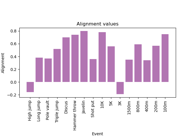
Figure 3(a) shows the alignment dendrogram between field events. The dendrogram consists of one dominant cluster of primarily throwing events and a smaller second cluster of jumping events. The first major cluster includes both genders’ hammer throw, discus, javelin, and shot put events. This major cluster consists of two subclusters, which exhibit more pronounced affinity within themselves. The second cluster consists of the men and women’s high jump and men’s long jump. Like Figure 3(b), the first difference behaviors are broadly grouped by event; this effect is more pronounced in track than field events. For example, the men and women’s 100 and 200m are closely clustered together, which may reflect substantial intersection in the athletes performing in these events.
This finding is by no means inevitable: one could imagine a scenario where the most similar behavior in these first differences is found between events within the same gender, that is, where athletic improvements are most closely associated among athletes competing of the same gender. This is shown not to be the case. Instead, the results in Figure 3 suggest that improvements are passed on rather uniformly between men and women. This could be due to breakthroughs in technology, technique, strength and conditioning, for each event, being passed on to men and women simultaneously.


VI Trajectory modelling and anomaly identification
Having observed broad similarity between (first differences in) scores between men and women in the same event in Section V, we now wish to approach the relationship between male and female scores differently and identify any events where there is relatively less consistency in scores. This section aims to study trends over time in scores, moving away from the first differences of the last section. As before, let be the multivariate time series consisting of the mean of the top women’s and men’s scores, respectively. While men and women are analyzed in conjunction, we never simultaneously compare track events to field events quantitatively, only descriptively, so our notation suppresses the dependence on these choices. Hence, rather than having total events, our notation denotes events separately for each of the track and field events.
To determine the consistency of evolutionary performance in men and women’s athletics events, we normalize each event’s time series for an appropriate comparison. To determine each men’s normalized trajectory we first compute , and then define . We similarly define women’s normalized trajectories . Then, we may compute distances between normalized trajectories by and , for men and women respectively. We remark that there are alternative ways to normalize such trajectories, such as subtracting the means and dividing by the ranges. As we use the metric to measure distances between the normalized trajectories, it makes consistent sense to use the norm in the normalization.
Next, we apply the linear transformation to both the men and women’s distance matrices, producing affinity matrices with all entries in . To determine the consistency in each event’s relative trajectory among the separate collections of men and women’s athletic events, we compute the consistency matrix . Specifically, Elements in the matrix close to 0 represent distances between events that are relatively similar among men and women. To determine the most inconsistent events, we compute and rank , for . Larger values indicate greater inconsistency between the male and female categories of the same events regarding their relationship with other events. We note that these distance, affinity and consistency matrices are computed separately for track and field events, so we suppress the dependence on this choice.
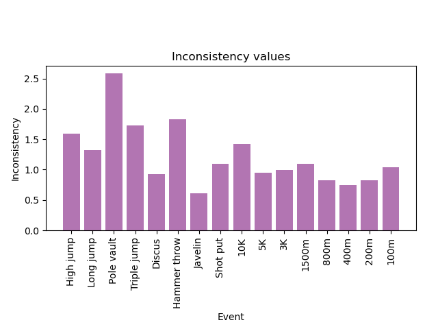
Figure 4 documents the inconsistency values of male and female trajectories in each event. The table highlights greater consistency in event trajectories among the track compared to the field events, with median values of 0.97 and 1.46, respectively. Field events display greater variability in their inconsistency values, with a standard deviation of 0.61, compared with 0.21 exhibited by track events. Indeed, both the most and least consistent events are field events, namely the javelin (inconsistency value of 0.61) and the pole vault (value of 2.58).


Figures 5(a) and 5(b) show the normalized trajectories of athletic scores over time for both men and women in the javelin and pole vault, respectively. It is evident from Figure 5 that the javelin exhibits highly similar trajectories for men and women - both feature a positive linear trend and rather uniform improvement with time. By contrast, the pole vault displays highly varying trends between genders. The women’s pole vault shows steady improvement in performance, while the men’s event exhibits a predominantly flat trajectory over time.
VII Geographic concentration analysis
Finally, we investigate trends in the composition of the top 100 scoring athletes in each event over time. Our data set records which country each athlete represents in the competitions, and we aim to produce and analyze a time-varying measure of the geographic diversity of athletes. For each event indexed and time we define an distance matrix between the top athletes’ locations. Specifically, let be the geodesic distance between the (centroids of the) countries of nationality of the and th athletes. For example, if all of the top athletes came from the same country in a given year, would be an matrix of zeroes. Larger values throughout the matrix indicate more geographic diversity of athletes, taking geographic locations into account. For an matrix , we use the Frobenius norm to quantify the total magnitude of the matrix, defined as .
For each event , we analyze the following function of time,
| (8) |
and compute the total geographic dispersion over time, defined by
| (9) |
measured in meters.

Our analysis highlights several trends in the variance of geographic representation among men and women’s events. All values of , quantifying the total geographic variance for each event, are recorded in Table 4. First, a highly similar geographic dispersion is identified between track and field events. The track events produce a mean (and median) value of 9.2 x 10⁶, while the field events produce a mean (and median) value of 8.8 x 10⁶. The most geographically concentrated track event is the women’s 200m, exhibiting a total value of 8.3 x 10⁶. The least concentrated track event is the women’s 5K, which produces a cumulative value of 9.8 x 10⁶. Among field events, men’s hammer throw consists of the most geographic concentration among the top 100 athletes, while the men’s long jump is the most geographically dispersed, with cumulative values of 7.2 x 10⁶ and 9.9 x 10⁶, respectively.
Second, a highly similar geographic dispersion is also observed between men and women’s events. The mean values among men and women are 9.0 x 10⁶ and 8.9 x 10⁶, respectively (with median values both 9.0 x 10⁶). Among men’s events, the most geographic variance in athletes is in the men’s long jump, while the greatest concentration is in the men’s hammer throw. Among female events, the greatest geographic concentration is in the 5K and 10K, with total values of 9.8 x 10⁶, while the least geographic dispersion among athletes is in the 200m and high jump, which both have cumulative values of 8.3 x 10⁶.
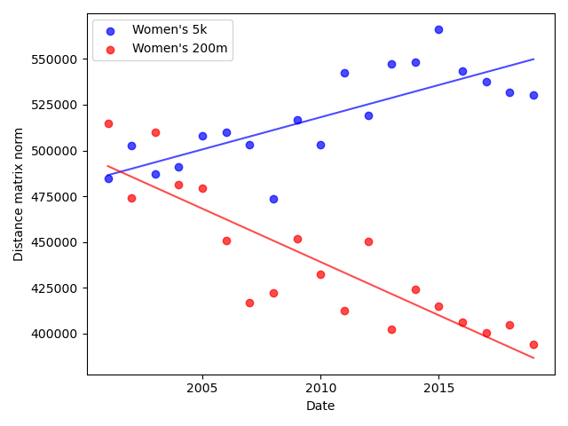
Figure 6 displays the time-varying geographic variance for the aforementioned events with the greatest and least total values. Three of these displayed events exhibit a moderate increase in geographic variance over time, but the women’s 200m exhibits a rather pronounced decrease. As a case study, we investigate the changing composition of this event. In Table 3, we perform a simple partition of women’s 200m athletes in 2001 and 2019 by continent of origin. This contrast confirms Figure 6(a), showing that the women’s 200m has become less geographically diverse over time, primarily due to a large number of athletes from the United States (US), 49 in 2019.
To investigate this further, we plot the number of US athletes among the top 100 as a function of time in Figure 7. Figure 1(b) depicts the counts for US athletes in the men and women’s 200m. To include a field event as well, Figure 7(b) depicts the analogous counts for the shot put. In each sport, we notice a considerable increase in the proportion of women athletes from the US.


| Continent | 2001 | 2019 |
|---|---|---|
| North America | 32 | 511 |
| Europe | 29 | 19 |
| Caribbean/Central America | 14 | 15 |
| Africa | 9 | 7 |
| Asia | 10 | 4 |
| South America | 3 | 6 |
| Oceania | 3 | 0 |
| Total geographic dispersion | |
|---|---|
| Event | |
| Men’s high jump | 8.9 x 10⁶ |
| Women’s high jump | 8.3 x 10⁶ |
| Men’s long jump | 9.9 x 10⁶ |
| Women’s long jump | 9.0 x 10⁶ |
| Men’s pole vault | 8.5 x 10⁶ |
| Women’s pole vault | 8.9 x 10⁶ |
| Men’s triple jump | 9.3 x 10⁶ |
| Women’s triple jump | 8.6 x 10⁶ |
| Men’s discus | 8.4 x 10⁶ |
| Women’s discus | 9.4 x 10⁶ |
| Men’s hammer throw | 7.2 x 10⁶ |
| Women’s hammer throw | 8.3 x 10⁶ |
| Men’s javelin | 8.7 x 10⁶ |
| Women’s javelin | 8.7 x 10⁶ |
| Men’s shot put | 8.8 x 10⁶ |
| Women’s shot put | 9.3 x 10⁶ |
| Men’s 10K | 9.7 x 10⁶ |
| Women’s 10K | 9.8 x 10⁶ |
| Men’s 5K | 8.6 x 10⁶ |
| Women’s 5K | 9.8 x 10⁶ |
| Men’s 3K | 9.0 x 10⁶ |
| Women’s 3K | 9.2 x 10⁶ |
| Men’s 1500m | 9.4 x 10⁶ |
| Women’s 1500m | 9.0 x 10⁶ |
| Men’s 800m | 9.4 x 10⁶ |
| Women’s 800m | 8.8 x 10⁶ |
| Men’s 400m | 9.8 x 10⁶ |
| Women’s 400m | 9.2 x 10⁶ |
| Men’s 200m | 9.2 x 10⁶ |
| Women’s 200m | 8.3 x 10⁶ |
| Men’s 100m | 9.0 x 10⁶ |
| Women’s 100m | 8.6 x 10⁶ |
VIII Conclusion
In this work, we have performed several quantitative analyses to identify patterns in the performance of athletes, the relationship between men and women’s trends within the same event, and the geographic composition of athletes over time.
This work takes a different approach to other quantitative analyses focused on modelling sport. Rather than modelling yearly performance data among a very small sample of results Wu et al. 2021; Einmahl and Magnus 2008; Robinson and Tawn 1995; Gembris, Taylor, and Suter 2002; Barão and Tawn 1999 (usually just the top scorer), this study is interested in broader patterns in performance. Furthermore, many of the techniques used throughout this paper may not provide the same level of insight when small annual samples of results lead to extremely volatile trends. Accordingly, throughout most of our analysis we study the top scorers per event per year.
First, in Section III, we implemented a regression analysis that revealed linear trends in improving average scores over time. By contrasting the fits of several models, we observed a positive Olympic effect in almost every event, where average scores are superior during Olympic years. While not necessarily surprising, this finding was by no means inevitable, as highly significant athletic events, such as the World Athletic Championships, occur more regularly. Nonetheless, it seems that the Olympic Games produce perhaps the highest levels of training and dedication to achieving the best scores possible. There may be several nuanced reasons for this effect. On the one hand, the increased media attention during the Olympics may increase performance; on the other hand, anxiety and stress may lead to decreased performances.Ott and Puymbroeck 2008
Next, we examined the linearity of these fits in more detail in Section IV. Perhaps surprisingly, and contrary to some recent reporting, Berthelot et al. 2010; McCurry 2021 we observed no evidence that average performance is “leveling off” close to the present day. This finding may differ with a careful analysis of world records, namely the single top athletic performance by year, but no evidence was observed when analyzing the top 100 athletes. We remark that there may be considerable limitations to analyzing just the single top performance. For example, no athlete has so far surpassed Usain Bolt’s world-record performance in the men’s 100m or 200m events, set in 2009. An incorporation of the top 100 athletes provides a better view of the holistic state of the elite performance in any candidate event. On the other hand, it is conceivable that incorporating more data, either further into the past or into the future could exhibit some leveling off.
We must also note that these two sections carry notable limitations and one should be cautious interpreting these results. For example, non-significant coefficients could be an artefact of the low number of data points (just 19) per event. More broadly, a significant coefficient (such as for the year-on-year improvement) is always more interpretable than a non-significant coefficient, which is not conclusive evidence of anything. The fact our methods do not broadly produce evidence of performance levelling off is related both to the choice of method and the question of study. Specifically, our methods (such as regression) work well in the context of studying average performances (mostly over the top athletes). They would not work as well focused specifically on the top scorer (). For this latter topic, many other papers have used quite different statistical techniques.Wu et al. 2021; Einmahl and Magnus 2008; Robinson and Tawn 1995; Gembris, Taylor, and Suter 2002; Barão and Tawn 1999
Continuing our study of the first differences, we observed substantial alignment between the men and women’s categories of each event in Section V. Even beyond the Olympic effect, men and women’s average scores moved in the same direction on a yearly basis to a considerable extent. Clustering based on our normalized inner products frequently paired men and women’s categories of the same events together. This suggests that sports may be characterized by improvements in technique and training that benefit the men and women’s competitions simultaneously. Interestingly, short and middle distance running exhibited pronounced similarity which may reflect the high degree of intersection in athlete registration among these events. For instance, it is not unusual for the same athlete to represent their country in the 100m and 200m or 200m and 400m. Usain Bolt of Jamaica and Michael Johnson of the US are two examples of such an overlap.
In Section VI, we took a different approach, this time seeking anomalies in the relationship between men and women’s categories of the same event. For this purpose, we investigated consistency in the normalized trajectories of scores with time. We were able to identify the pole vault and javelin as the events with the greatest and least consistency in the trajectories of men and women’s events. We failed to identify higher levels of structure among our trajectory anomalies.
Finally, Section VII turned our attention to the athletes themselves, specifically their countries of origin and the changing composition of events over time. Here, we obtained a surprising result: a high degree of similarity in geographic variance across all studied events, track and field, men and women. This may counter a popular conception that certain events are more dominated by smaller selections of countries, such as sprint events by athletes from the US and Jamaica.Brooks 2014 Instead, with some exceptions, almost every event exhibited proportionate variance of athletes from across the world. Some trends in changing levels of geographic variance over time were observed, particularly for some women’s events. Future work can study the proportion of athletes from the US and investigate whether this proportion is increasing, especially in women’s events.
Overall, this work introduces methods to study the evolution of elite athletes’ performance over the past two decades. We identify structural similarities and dissimilarities among various track and field events and the performance of men and women. In addition, we highlight surprising homogeneity in time-varying geographic composition among various events’ athletic representation. Although these methods were developed for this application specifically, we believe that our techniques could be applied beyond athletics and more broadly beyond competitive sport. Researchers interested in identifying structure in any phenomenon evolving over time and comparing the evolutionary performance of subgroups could apply these techniques effectively.
Data availability
The data that support the findings of this study are openly available at Ref. oly 2021.
Acknowledgements.
The authors would like to thank Kirsten Doert Eccles from the Melbourne Centre for Data Science, who first proposed the idea on writing a paper studying human performance and the Olympics. The authors would also like to thank Nathaniel Bloomfield for his help in accessing the data.Appendix A Supplementary experiments on the linear regression
In Figure 8, we demonstrate the homoscedasticity of residuals for a collection of events, complementing the linear regressions performed in Section III. The plots show in most cases that residuals are satisfactorily distributed with mean zero and rather constant variance.
In Tables 5, 6 and 7, respectively, we document Akaike information criteria (AIC) and Bayesian information criteria (BIC) scores Vrieze 2012 for each of Models 1,2 and 3 from Section III.


| Model 1 AIC and BIC | ||||
|---|---|---|---|---|
| Event | AIC | AIC | BIC | BIC |
| Men’s high jump | -147.2 | -113.8 | -145.3 | -111.9 |
| Women’s high jump | -145.5 | -116.6 | -143.6 | -114.7 |
| Men’s long jump | -94.2 | -66.6 | -92.4 | -64.7 |
| Women’s long jump | -81.3 | -59.5 | -79.4 | -57.6 |
| Men’s pole vault | -85.4 | -77.7 | -83.5 | -75.8 |
| Women’s pole vault | -86.3 | -66.9 | -84.4 | -65.0 |
| Men’s triple jump | -50.9 | -46.2 | -49.0 | -44.4 |
| Women’s triple jump | -47.0 | -26.5 | -45.1 | -24.6 |
| Men’s discus | 14.2 | 34.2 | 16.1 | 36.0 |
| Women’s discus | 24.7 | 37.0 | 26.6 | 38.9 |
| Men’s hammer throw | 19.5 | 26.8 | 21.4 | 28.7 |
| Women’s hammer throw | 50.8 | 60.4 | 52.7 | 62.3 |
| Men’s javelin | 27.3 | 58.7 | 29.2 | 60.6 |
| Women’s javelin | 15.4 | 26.1 | 17.3 | 27.9 |
| Men’s shot put | -25.8 | -7.5 | -23.9 | -5.6 |
| Women’s shot put | -24.3 | -13.8 | -22.5 | -11.9 |
| Men’s 10K | 132.8 | 142.8 | 134.7 | 144.7 |
| Women’s 10K | 149.1 | 176.4 | 150.1 | 178.2 |
| Men’s 5K | 85.6 | 98.7 | 87.5 | 100.6 |
| Women’s 5K | 107 | 104.5 | 108.9 | 106.3 |
| Men’s 3K | 75.4 | 83.6 | 77.3 | 85.5 |
| Women’s 3K | 101.1 | 124.5 | 103.0 | 126.4 |
| Men’s 1500m | 19.4 | 42.0 | 21.3 | 43.9 |
| Women’s 1500m | 29.0 | 57.7 | 30.1 | 59.6 |
| Men’s 800m | -21.5 | 15.9 | -19.6 | 17.8 |
| Women’s 800m | 2.4 | 30.5 | 4.3 | 32.4 |
| Men’s 400m | -38.1 | -14.2 | -36.2 | -12.3 |
| Women’s 400m | -19.7 | -10.8 | -17.8 | -8.9 |
| Men’s 200m | -74.3 | -51.3 | -72.4 | -49.4 |
| Women’s 200m | -55.1 | -37.4 | -53.2 | -35.5 |
| Men’s 100m | -99.0 | -68.0 | -97.1 | -66.1 |
| Women’s 100m | -92.2 | -65.7 | -90.3 | -63.8 |
| Model 2 AIC and BIC | ||||
|---|---|---|---|---|
| Event | AIC | AIC | BIC | BIC |
| Men’s high jump | -148.8 | -113.3 | -145.9 | -110.5 |
| Women’s high jump | -147.2 | -116.3 | -144.4 | -113.5 |
| Men’s long jump | -94.7 | -65.0 | -91.9 | -62.1 |
| Women’s long jump | -86.8 | -68.1 | -83.9 | -65.3 |
| Men’s pole vault | -85.1 | -75.8 | -82.3 | -72.9 |
| Women’s pole vault | -93.8 | -70.0 | -90.9 | -67.0 |
| Men’s triple jump | -53.7 | -44.5 | -50.1 | -41.7 |
| Women’s triple jump | -51.7 | -33.7 | -48.8 | -30.9 |
| Men’s discus | -2.8 | 34.9 | 0.07 | 37.7 |
| Women’s discus | 12.3 | 37.7 | 15.1 | 40.5 |
| Men’s hammer throw | 5.4 | 26.0 | 8.2 | 28.8 |
| Women’s hammer throw | 45.4 | 61.3 | 48.2 | 64.1 |
| Men’s javelin | 27.5 | 59.3 | 30.3 | 62.2 |
| Women’s javelin | 10.3 | 27.0 | 13.1 | 29.9 |
| Men’s shot put | -26.2 | -6.1 | -23.4 | -3.3 |
| Women’s shot put | -27.6 | -22.2 | -24.7 | -19.4 |
| Men’s 10K | 127.4 | 143.5 | 130.3 | 146.3 |
| Women’s 10K | 145.4 | 173.3 | 148.2 | 176.1 |
| Men’s 5K | 84.8 | 100.4 | 87.7 | 103.2 |
| Women’s 5K | 104.7 | 106 | 107.5 | 108.8 |
| Men’s 3K | 75.0 | 85.5 | 77.9 | 88.4 |
| Women’s 3K | 102.1 | 124.9 | 104.9 | 127.7 |
| Men’s 1500m | 19.8 | 43.5 | 22.7 | 46.4 |
| Women’s 1500m | 29.1 | 59.7 | 31.9 | 62.6 |
| Men’s 800m | -24.5 | 16.2 | -21.7 | 19.1 |
| Women’s 800m | -8.9 | 26.2 | -6.1 | 29.1 |
| Men’s 400m | -36.3 | -12.5 | -33.5 | -9.7 |
| Women’s 400m | -24.8 | -10.6 | -22 | -7.7 |
| Men’s 200m | -73.1 | -49.7 | -70.2 | -46.8 |
| Women’s 200m | -66.9 | -42.3 | -64.0 | -39.4 |
| Men’s 100m | -103.8 | -69.4 | -101 | -66.6 |
| Women’s 100m | -94.9 | -71.3 | -92.1 | -68.4 |
| Model 3 AIC and BIC | ||||
|---|---|---|---|---|
| Event | AIC | AIC | BIC | BIC |
| Men’s high jump | -145.4 | -109.5 | -140.7 | -104.8 |
| Women’s high jump | -152.1 | -118.3 | 147.4 | 113.6 |
| Men’s long jump | -92.5 | -61.0 | -87.8 | -56.3 |
| Women’s long jump | -91.3 | -66.6 | -86.6 | -61.9 |
| Men’s pole vault | -82.7 | -73.8 | -78.0 | -69.1 |
| Women’s pole vault | -92.8 | -68.8 | -88.1 | -64.1 |
| Men’s triple jump | -51.3 | -44.7 | -46.6 | -40.0 |
| Women’s triple jump | -51.2 | -34.6 | -46.4 | -29.9 |
| Men’s discus | 0.70 | 37.5 | 5.4 | 42.3 |
| Women’s discus | 14.4 | 41.5 | 19.1 | 46.2 |
| Men’s hammer throw | 1.1 | 25.5 | 5.8 | 30.2 |
| Women’s hammer throw | 47.2 | 65.2 | 52.0 | 69.9 |
| Men’s javelin | 30.8 | 63.3 | 35.6 | 68.0 |
| Women’s javelin | 13.7 | 27.5 | 18.4 | 32.2 |
| Men’s shot put | -22.9 | -3.8 | -18.2 | .98 |
| Women’s shot put | -24.0 | -18.4 | -19.3 | -13.7 |
| Men’s 10K | 117.0 | 139.7 | 121.7 | 144.4 |
| Women’s 10K | 143.9 | 173.8 | 148.6 | 178.5 |
| Men’s 5K | 88.7 | 103 | 93.4 | 107.7 |
| Women’s 5K | 106.6 | 108.7 | 111.3 | 113.4 |
| Men’s 3K | 74.6 | 87.3 | 79.4 | 92.0 |
| Women’s 3K | 99.2 | 125.9 | 103.9 | 130.6 |
| Men’s 1500m | 18.8 | 47.2 | 23.6 | 51.9 |
| Women’s 1500m | 33.0 | 63.2 | 37.7 | 67.9 |
| Men’s 800m | -21.6 | 17.4 | -16.9 | 22.1 |
| Women’s 800m | -5.3 | 29.3 | -.55 | 34.0 |
| Men’s 400m | -33.6 | -9.6 | -28.9 | -4.9 |
| Women’s 400m | -21.5 | -8.5 | -16.8 | -3.7 |
| Men’s 200m | -70.6 | -50.3 | -65.9 | -45.6 |
| Women’s 200m | -64.0 | -39.3 | -59.3 | -34.6 |
| Men’s 100m | -103.4 | -66.0 | -98.7 | -61.2 |
| Women’s 100m | -95.8 | -76.0 | -91.1 | -71.2 |
Appendix B Geographic Variance Gini
In Figure 9, we complement our study of geographic variation in Section VII with a more straightforward measure of athletes’ diversity of nationalities each year. We display computed Gini coefficients for track and field events, both according to the top 100 and 10 scorers each year. Compared to Section VII, we see slightly more variability between different events. These different results can be explained by the different method of calculation, which does not take into account geographic dispersion.


References
- Elderton and Wood (1945) W. Elderton and G. H. Wood, “Cricket scores and some skew correlation distributions: (an arithmetical study),” Journal of the Royal Statistical Society 108, 1 (1945).
- Kimber and Hansford (1993) A. C. Kimber and A. R. Hansford, “A statistical analysis of batting in cricket,” Journal of the Royal Statistical Society. Series A (Statistics in Society) 156, 443 (1993).
- Gabel and Redner (2012) A. Gabel and S. Redner, “Random walk picture of basketball scoring,” Journal of Quantitative Analysis in Sports 8 (2012), 10.1515/1559-0410.1416.
- Pawlowski (2013) T. Pawlowski, “Testing the uncertainty of outcome hypothesis in european professional football,” Journal of Sports Economics 14, 341–367 (2013).
- Wu et al. (2021) P. P.-Y. Wu, L. Garufi, C. Drovandi, K. Mengersen, L. J. Mitchell, M. A. Osborne, and D. B. Pyne, “Bayesian prediction of winning times for elite swimming events,” Journal of Sports Sciences , 1–8 (2021).
- Einmahl and Magnus (2008) J. H. J. Einmahl and J. R. Magnus, “Records in athletics through extreme-value theory,” Journal of the American Statistical Association 103, 1382–1391 (2008).
- Robinson and Tawn (1995) M. E. Robinson and J. A. Tawn, “Statistics for exceptional athletics records,” Applied Statistics 44, 499 (1995).
- Gembris, Taylor, and Suter (2002) D. Gembris, J. G. Taylor, and D. Suter, “Trends and random fluctuations in athletics,” Nature 417, 506–506 (2002).
- Barão and Tawn (1999) M. I. Barão and J. A. Tawn, “Extremal analysis of short series with outliers: sea-levels and athletics records,” Journal of the Royal Statistical Society: Series C (Applied Statistics) 48, 469–487 (1999).
- Ribeiro, Mukherjee, and Zeng (2012) H. V. Ribeiro, S. Mukherjee, and X. H. T. Zeng, “Anomalous diffusion and long-range correlations in the score evolution of the game of cricket,” Physical Review E 86 (2012), 10.1103/physreve.86.022102.
- Merritt and Clauset (2014) S. Merritt and A. Clauset, “Scoring dynamics across professional team sports: tempo, balance and predictability,” EPJ Data Science 3 (2014), 10.1140/epjds29.
- Clauset, Kogan, and Redner (2015) A. Clauset, M. Kogan, and S. Redner, “Safe leads and lead changes in competitive team sports,” Physical Review E 91 (2015), 10.1103/physreve.91.062815.
- Kiley et al. (2016) D. P. Kiley, A. J. Reagan, L. Mitchell, C. M. Danforth, and P. S. Dodds, “Game story space of professional sports: Australian rules football,” Physical Review E 93 (2016), 10.1103/physreve.93.052314.
- James, Menzies, and Bondell (2022) N. James, M. Menzies, and H. Bondell, “Comparing the dynamics of COVID-19 infection and mortality in the United States, India, and Brazil,” Physica D: Nonlinear Phenomena 432, 133158 (2022).
- James and Menzies (2020) N. James and M. Menzies, “COVID-19 in the United States: Trajectories and second surge behavior,” Chaos: An Interdisciplinary Journal of Nonlinear Science 30, 091102 (2020).
- Chowell et al. (2016) G. Chowell, L. Sattenspiel, S. Bansal, and C. Viboud, “Mathematical models to characterize early epidemic growth: A review,” Physics of Life Reviews 18, 66–97 (2016).
- James, Menzies, and Radchenko (2021) N. James, M. Menzies, and P. Radchenko, “COVID-19 second wave mortality in Europe and the United States,” Chaos: An Interdisciplinary Journal of Nonlinear Science 31, 031105 (2021).
- Manchein et al. (2020) C. Manchein, E. L. Brugnago, R. M. da Silva, C. F. O. Mendes, and M. W. Beims, “Strong correlations between power-law growth of COVID-19 in four continents and the inefficiency of soft quarantine strategies,” Chaos: An Interdisciplinary Journal of Nonlinear Science 30, 041102 (2020).
- Blasius (2020) B. Blasius, “Power-law distribution in the number of confirmed COVID-19 cases,” Chaos: An Interdisciplinary Journal of Nonlinear Science 30, 093123 (2020).
- James and Menzies (2021a) N. James and M. Menzies, “Trends in COVID-19 prevalence and mortality: A year in review,” Physica D: Nonlinear Phenomena 425, 132968 (2021a).
- James and Menzies (2022a) N. James and M. Menzies, “Estimating a continuously varying offset between multivariate time series with application to COVID-19 in the United States,” The European Physical Journal Special Topics (2022a), 10.1140/epjs/s11734-022-00430-y.
- Drożdż et al. (2020a) S. Drożdż, J. Kwapień, P. Oświęcimka, T. Stanisz, and M. Wątorek, “Complexity in economic and social systems: Cryptocurrency market at around COVID-19,” Entropy 22, 1043 (2020a).
- James and Menzies (2021b) N. James and M. Menzies, “Association between COVID-19 cases and international equity indices,” Physica D: Nonlinear Phenomena 417, 132809 (2021b).
- Drożdż, Kwapień, and Oświęcimka (2021) S. Drożdż, J. Kwapień, and P. Oświęcimka, “Complexity in economic and social systems,” Entropy 23, 133 (2021).
- James and Menzies (2021c) N. James and M. Menzies, “Efficiency of communities and financial markets during the 2020 pandemic,” Chaos: An Interdisciplinary Journal of Nonlinear Science 31, 083116 (2021c).
- Drożdż et al. (2020b) S. Drożdż, L. Minati, P. Oświęcimka, M. Stanuszek, and M. Wątorek, “Competition of noise and collectivity in global cryptocurrency trading: Route to a self-contained market,” Chaos: An Interdisciplinary Journal of Nonlinear Science 30, 023122 (2020b).
- James and Menzies (2021d) N. James and M. Menzies, “A new measure between sets of probability distributions with applications to erratic financial behavior,” Journal of Statistical Mechanics: Theory and Experiment 2021, 123404 (2021d).
- Wątorek et al. (2020) M. Wątorek, S. Drożdż, J. Kwapień, L. Minati, P. Oświęcimka, and M. Stanuszek, “Multiscale characteristics of the emerging global cryptocurrency market,” Physics Reports (2020), 10.1016/j.physrep.2020.10.005.
- Prakash et al. (2022) A. Prakash, N. James, M. Menzies, and G. Francis, “Structural clustering of volatility regimes for dynamic trading strategies,” Applied Mathematical Finance (2022), 10.1080/1350486X.2021.2007146.
- Vazquez (2006) A. Vazquez, “Polynomial growth in branching processes with diverging reproductive number,” Physical Review Letters 96 (2006), 10.1103/physrevlett.96.038702.
- Mendes and Beims (2018) C. F. Mendes and M. W. Beims, “Distance correlation detecting Lyapunov instabilities, noise-induced escape times and mixing,” Physica A: Statistical Mechanics and its Applications 512, 721–730 (2018).
- Shang et al. (2020) K. Shang, B. Yang, J. M. Moore, Q. Ji, and M. Small, “Growing networks with communities: A distributive link model,” Chaos: An Interdisciplinary Journal of Nonlinear Science 30, 041101 (2020).
- Hethcote (2000) H. W. Hethcote, “The mathematics of infectious diseases,” SIAM Review 42, 599–653 (2000).
- Perc et al. (2020) M. Perc, N. G. Miksić, M. Slavinec, and A. Stožer, “Forecasting COVID-19,” Frontiers in Physics 8, 127 (2020).
- Moeckel and Murray (1997) R. Moeckel and B. Murray, “Measuring the distance between time series,” Physica D: Nonlinear Phenomena 102, 187–194 (1997).
- Székely, Rizzo, and Bakirov (2007) G. J. Székely, M. L. Rizzo, and N. K. Bakirov, “Measuring and testing dependence by correlation of distances,” The Annals of Statistics 35, 2769–2794 (2007).
- Mendes, da Silva, and Beims (2019) C. F. O. Mendes, R. M. da Silva, and M. W. Beims, “Decay of the distance autocorrelation and Lyapunov exponents,” Physical Review E 99 (2019), 10.1103/physreve.99.062206.
- James et al. (2020) N. James, M. Menzies, L. Azizi, and J. Chan, “Novel semi-metrics for multivariate change point analysis and anomaly detection,” Physica D: Nonlinear Phenomena 412, 132636 (2020).
- Karaivanov (2020) A. Karaivanov, “A social network model of COVID-19,” PLOS ONE 15, e0240878 (2020).
- Ge et al. (2020) J. Ge, D. He, Z. Lin, H. Zhu, and Z. Zhuang, “Four-tier response system and spatial propagation of COVID-19 in China by a network model,” Mathematical Biosciences 330, 108484 (2020).
- Xue et al. (2020) L. Xue, S. Jing, J. C. Miller, W. Sun, H. Li, J. G. Estrada-Franco, J. M. Hyman, and H. Zhu, “A data-driven network model for the emerging COVID-19 epidemics in Wuhan, Toronto and Italy,” Mathematical Biosciences 326, 108391 (2020).
- Machado and Lopes (2020) J. A. T. Machado and A. M. Lopes, “Rare and extreme events: the case of COVID-19 pandemic,” Nonlinear Dynamics (2020), 10.1007/s11071-020-05680-w.
- Ngonghala, Iboi, and Gumel (2020) C. N. Ngonghala, E. A. Iboi, and A. B. Gumel, “Could masks curtail the post-lockdown resurgence of COVID-19 in the US?” Mathematical Biosciences 329, 108452 (2020).
- Cavataio and Schnell (2021) J. Cavataio and S. Schnell, “Interpreting SARS-CoV-2 seroprevalence, deaths, and fatality rate — making a case for standardized reporting to improve communication,” Mathematical Biosciences 333, 108545 (2021).
- Náraigh and Byrne (2020) L. Ó. Náraigh and Á. Byrne, “Piecewise-constant optimal control strategies for controlling the outbreak of COVID-19 in the Irish population,” Mathematical Biosciences 330, 108496 (2020).
- Glass (2020) D. H. Glass, “European and US lockdowns and second waves during the COVID-19 pandemic,” Mathematical Biosciences 330, 108472 (2020).
- Hastie, Tibshirani, and Friedman (2009) T. Hastie, R. Tibshirani, and J. Friedman, The Elements of Statistical Learning (Springer New York, 2009).
- Nguefack et al. (2020) H. L. N. Nguefack, M. G. Pagé, J. Katz, M. Choinière, A. Vanasse, M. Dorais, O. M. Samb, and A. Lacasse, “Trajectory modelling techniques useful to epidemiological research: A comparative narrative review of approaches,” Clinical Epidemiology Volume 12, 1205–1222 (2020).
- Nagin (2014) D. S. Nagin, “Group-based trajectory modeling: An overview,” Annals of Nutrition and Metabolism 65, 205–210 (2014).
- James, Menzies, and Chan (2021) N. James, M. Menzies, and J. Chan, “Changes to the extreme and erratic behaviour of cryptocurrencies during COVID-19,” Physica A: Statistical Mechanics and its Applications 565, 125581 (2021).
- James and Menzies (2022b) N. James and M. Menzies, “Collective correlations, dynamics, and behavioural inconsistencies of the cryptocurrency market over time,” Nonlinear Dynamics (2022b), 10.1007/s11071-021-07166-9.
- Müllner (2013) D. Müllner, “Fastcluster: Fast hierarchical, agglomerative clustering routines forRandPython,” Journal of Statistical Software 53 (2013), 10.18637/jss.v053.i09.
- James, Menzies, and Bondell (2021) N. James, M. Menzies, and H. Bondell, “Understanding spatial propagation using metric geometry with application to the spread of COVID-19 in the United States,” EPL (Europhysics Letters) (2021), 10.1209/0295-5075/ac2752.
- oly (2021) “World athletics home page,” https://www.worldathletics.org/records/toplists/ (2021), World Athletics, Accessed September 1, 2021.
- Ott and Puymbroeck (2008) K. Ott and M. V. Puymbroeck, “Does the media impact athletic performance?” https://thesportjournal.org/article/does-the-media-impact-athletic-performance/ (2008), The Sport Journal, March 14, 2008.
- Berthelot et al. (2010) G. Berthelot et al., “Athlete atypicity on the edge of human achievement: Performances stagnate after the last peak, in 1988,” PLoS ONE 5, e8800 (2010).
- McCurry (2021) J. McCurry, “As Olympic athletics begins, the data suggests we are at the peak of human ability,” https://www.theguardian.com/business/grogonomics/2021/jul/29/as-olympic-athletics-begins-the-data-suggests-we-are-at-the-peak-of-human-ability (2021), The Guardian, July 29, 2021.
- Brooks (2014) M. Brooks, “Why are Jamaicans so good at sprinting?” https://www.theguardian.com/commentisfree/2014/jul/21/jamaicans-sprinting-athletics-commonwealth-games (2014), The Guardian, July 21, 2014.
- Vrieze (2012) S. I. Vrieze, “Model selection and psychological theory: A discussion of the differences between the Akaike information criterion (AIC) and the Bayesian information criterion (BIC).” Psychological Methods 17, 228–243 (2012).