Random Dilated Shapelet Transform: A New Approach for Time Series Shapelets

We present a brief overview of the algorithms identified as state-of-the-art and used in our experimental section, and we report the reader to a recent review [1] for a more detailed view of the field.

• •

  Shapelet Transform Classifier (STC) [2], is regarded as a state of the art for shapelet algorithms in terms of accuracy. This algorithm iteratively initializes new shapelets, assesses their discriminative power, and removes those that are too similar. The goal being to maximize the discriminative power of an ensemble of shapelets. A Rotation Forest is then applied as a classifier.

• •

  Temporal Dictionary Ensemble (TDE) [17] is an ensemble of dictionary-based classifiers. It uses some variants of the BOSS classifier [20] and WEASEL [21], as base estimators and optimizes their parameters through a Gaussian process.

• •

  Diverse Representation Canonical Interval Forest Classifier (DrCIF) [18], is an extension of the CIF algorithm [16]. After selecting random intervals from different representations of the time series, it uses the Catch22 [14] method to extract a feature matrix.

• •

  RandOm Convolutional KErnel Transform (ROCKET) [4], randomly generates a huge set of convolutional kernels, and extracts as features the maximum and the proportion of positive values of the convolution for each time series and each kernel. It is followed by a Ridge classifier. An ensemble version of this method, called ARSENAL, was introduced by [18].

• •

  Inception-Time [10] is an ensemble of Inception networks, which introduce Inception modules as replacement for traditional fully convolutional layers, notably to mitigate the vanishing gradient problem.

• •

  Hierarchical Vote Collective of Transformation-based Ensembles (HC1) [13]is a meta-ensemble classifier using a variety of time series classifiers, such as STC, with a novel ensemble learning scheme which estimate the weight of each base classifier in the final decision. This estimation is based on performance in a 10-fold validation scheme.

  Variants of this method were developed, such as TS-CHIEF [22] and HC2 [18], that both modify the set of base classifiers to improve accuracy. HC2 also modified the meta-ensemble procedure, using a Out-Of-Bag estimate instead of a 10-fold validation to estimate the performance of each base classifier, which improved scalability compared to HC1.

Shapelets [25] were originally defined as time series subsequences representative of class membership. In the following, we define a shapelet $S$ as a vector $S=\{s_{1},...,s_{l}\}$ with $l$ its length. All shapelet-based algorithms have the same protocol to extract features from a shapelet $S$ and a time series $X=\{x_{1},...,x_{m}\}$, by using a distance vector $f(S,X)=\{f_{1},...,f_{m-(l-1)}\}$ defined as :

In this definition, a point $f_{i}$ is simply the Euclidean distance between $S$ and the subsequence of length $l$ starting at index $i$ in $X$. The minimum value of $f(S,X)$ is then extracted as a feature, which can be interpreted as an indicator of the presence of the pattern represented by $S$ in $X$. A popular variant of this distance function consists in using a z-normalized Euclidean distance, where $S$ and all subsequences of $X$ are z-normalized independently, allowing to add scale invariance to the translation invariance of the initial formulation. Then, as presented in the Shapelet Transform [12], by using a set of shapelets $\cal S$, one can then transform an ensemble of time series $\cal X$ into a feature matrix of shape $(|{\cal X}|,|{\cal S}|)$, and use it as input in a non-temporal classifier such as a decision tree.

The step of generating and selecting shapelet candidates is the main difference between most approaches. In order to speed up the exhaustive search, Fast Shapelet [11] use input discretization, while Ultra Fast Shapelet [24] use random sampling. FLAG [8] build shapelets location indicators from the data to reduce the set of admissible candidates, and GENDIS [23] use an evolutionary algorithm initialized by a clustering on the set of possible candidates. Learning Time Series Shapelet [6] use a gradient-descent optimization that iteratively change the values of a set of shapelets. MrSEQL [19], while not strictly speaking a shapelet algorithm, searches for discriminative symbolic sequences in a variety of symbolic representations of the inputs.

Since the publication of Localized Random Shapelet (LRS) [7], which showed the benefit of extracting $argmin\ d(S,X)$ to discriminate time series based on the location of the minimum between $S$ and $X$, it has been included in most recent approaches. Based on their results, we will also use this feature in our method.

To introduce the notion of dilation in shapelets, we define now a shapelet $S$ as $S=\{\{v_{1},...,v_{l}\},d\}$ with $l$ the length parameter and $d$ the dilation parameter. In practice, the dilation is used in the distance function $f$, where each value of the shapelet will be compared to a dilated subsequence of the input time series. More formally, consider a time series $X=\{x_{1},...,x_{m}\}$ and a dilated shapelet $S$, we now define $f(S,X)=\{f_{1},...,f_{m-(l-1)\times d}\}$ as :

The interest of using dilation in shapelets is to make them non-contiguous subsequences. It allows a shapelet to either match a non-contiguous pattern, or a contiguous one, by focusing on key points of the pattern without covering it entirely, as illustrated in Figure 1. Note that this formulation is equivalent to the original shapelet formulation when $d=1$.

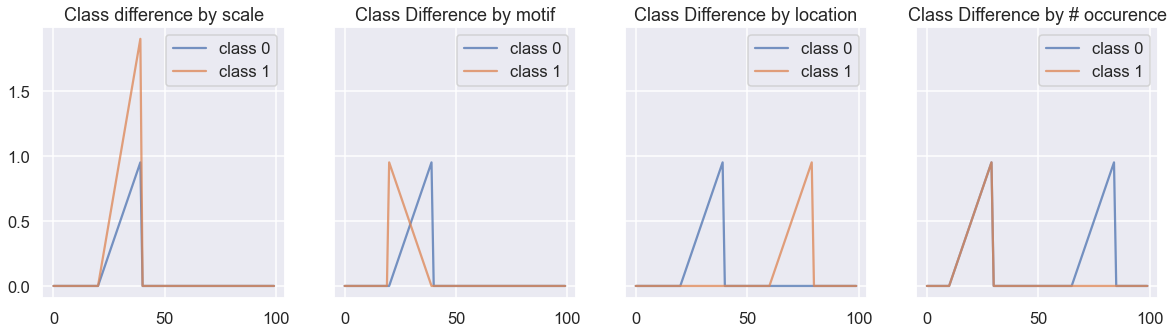
If we consider a shapelet $S$ and two time series $X_{1}$ and $X_{2}$, we can imagine multiple ways of discriminating $X_{1}$ and $X_{2}$ using $S$.

• •

  $S$ can be present in $X_{1}$ but not in $X_{2}$. This is captured by $min\ f(S,X_{i})$, with smaller distances indicating better matches between the shapelet and the series.

• •

  $S$ can be present in both series, but not at the same place. This is captured by the $argmin$ feature introduced by LRS [7].

• •

  $S$ can be present in both series, but not at the same scale. In this case, a normalized distance would not be able to discriminate the series.

• •

  $S$ can be present in both series, but occurs a different number of times in $X_{1}$ compared to $X_{2}$. This is captured by a new feature, called Shapelet Occurrence (SO).

Those points are illustrated in Figure 2. Deciding whether scaling is important or not is highly dependent on the application, but without prior knowledge, one cannot know which to choose. For this reason, we introduce a parameter in Section 3.3 allowing to tune the amount of normalized shapelets.

To the best of our knowledge, the number of occurrences of a shapelet has never been considered as a feature. This requires another modification to the definition of $S$ as $S=\{\{v_{1},...,v_{l}\},d,\lambda\}$, with $\lambda$ a threshold allowing us to compute the Shapelet Occurrence ($SO$) feature as $SO=|\{i|f(S,X)_{i}<\lambda\}|$. Although the parameter $\lambda$ could be set randomly, we discuss in Section 3.3 a method to set the value of this threshold.

Our objective for this algorithm is to produce an accurate but scalable approach. As our shapelet formulation adds attributes compared to the initial formulation [25], optimizing a set of dilated shapelets with a threshold $\lambda$ will be costly, and this explains why we choose a random approach.

For simplicity, we present our approach in the context of univariate and even length time series, with ${\cal X}=\{X_{1},...,X_{n}\}$ a set of time series ($X_{i}=\{x_{1},...,x_{m}\}$) and $Y=\{y_{1},...,y_{n}\}$ their respective classes. Our method takes as input four parameters that are: $n\_shapelets$ the number of shapelets to generate, $L$ a set of possible lengths for the shapelets, $p\_norm$ the proportion of shapelets that will use z-normalization, and $(P_{1},P_{2})\in[0,100]$ a pair used as percentile bounds for the sampling of the threshold $\lambda$.

Given the definition of a shapelet $S=\{\{v_{1},...,v_{l}\},d,\lambda\}$, we initialize each parameter as follows:

• •

  the length $l$ is uniformly drawn from $L$,

• •

  the dilation $d$, in the same way as ROCKET [4], is set to $d=\left\lfloor 2^{x}\right\rfloor$ with $x$ uniformly drawn in $[0,log_{2}\frac{m}{l}]$,

• •

  we randomly choose whether the shapelet will use a z-normalized distance with probability $p\_norm$,

• •

  for setting the values, a sample $X$ is uniformly drawn from ${\cal X}$, and an admissible start point $i$ (given $l,d$) is randomly selected. Then, values are set to $[X_{i},...,X_{i+(l-1)\times d}]$.

• •

  finally, given a shapelet $S$, to fix the value of $\lambda$, we take a sample $X$ from the same class as the one used for extracting the shapelet value, and uniformly draw a value between the two percentiles $(P_{1},P_{2})$ of $f(S,X)$.

The strategy employed to find $\lambda$ is a classic trade-off between time and accuracy. If scalability was not a focus, we could compute the distance vector for more samples in ${\cal X}$, and optimize the value of $\lambda$ based on an information measure. After computing the distance vector between all pairs of time series and shapelets, the output of our method is a feature matrix of size $(|{\cal X}|,3\times n\_shapelets)$, with the three features extracted from the distance vector $f(S,X)$ being the $min,argmin,SO(S,X)$.

Following the arguments of the authors of ROCKET [4], we use a Ridge Classifier after the transformation of ${\cal X}$, as the L2 regularization used in Ridge is of critical importance due to the high number of features that are generated, while being scalable and interpretable.

We conduct a sensitivity analysis on the four input parameters of our algorithm and their effect on classification accuracy on 40 datasets selected randomly, with raw results and selected datasets in a specific file in the online repository. For each parameter analysis, all other parameters remain fixed at the following default values : $n\_shapelets=10000$, $p\_norm=0.9$, $L=[7,9,11]$, $P1=5$ and $P2=15$. Figure 3 and Figure 4 give the mean accuracy ranks of each method over the 40 datasets, with the accuracy of each method and each dataset computed as the mean of the same 10 resamples. Given the tested set of values, the most impactful parameter is the number of shapelets, with a noticeable increase in performance above 10000 shapelets. All other parameters only display minor gains and thus seem to be stable. Based on those results, for all further experiments we set as default parameters $n\_shapelets=10000$, $p\_norm=0.8$, $L=[11]$ and $P1=5$, $P2=10$, and report results for datasets used in sensitivity analysis and the others.

We perform a comparison of the scalability of our approach against Hive-Cote 1.0 (HC1), Hive-Cote 2.0 (HC2), DrCIF, ROCKET, and the Shapelet Transform Classifier (STC). Note that when used as a component in HC1 and HC2, STC is by default subject to a time contract of two hours. Except from this default configuration in HC1 and HC2, we are not setting any time contract in other algorithms. Both STC and RDST are by default sampling 10000 shapelets, and ROCKET use 10000 kernels.

We are aware that the runtime of HC1, HC2 and STC could be reduced with time contracts. But, as our goal in this section is to contextualize the gain in classification accuracy against the time complexity of each method, we present the results with the time contracts used to generate the accuracy results of the next section.

We use the Crop Dataset and the Rock Dataset of the UCR archive for evaluating the scalability respectively on the number of time series and their length. As all competing algorithms implemented in the sktime package of [15] can use parallel processing, we set each algorithm to use 90 cores. Figure 5 reports the mean training time over 10 resamples, showing the very competitive scalability of RDST. Note that due to job time limitation on our machine and the computational cost of HC2, we could not consider all samples for the Crop dataset. We report the reader interested in the implementation details of our algorithm to the web page of the project.

We present the results of our comparative study using the mean accuracy over the same 30 resamples for each of the 112 datasets as HC2 [18] used in their study, and compare our approach against their experimental result. Figure 6 gives the mean accuracy rank of each method over the 40 datasets used for setting the defaults parameters in sensitivity analysis, and for the 72 others. The full result tables including standard deviation per dataset and more visualizations of the results are available online as supplementary materials.

Given the scalability and simplicity of our method, having an accuracy comparable to the prior developments of HC2 and to deep learning approaches is a very promising result. Notably for future developments where focus would shift to accuracy rather than scalability. For reference, using RDST without any distance normalization is equivalent to STC in terms of mean accuracy rank, with the same protocol as above.

Given a set of $M$ shapelets, RDST generates $3M$ features. Each feature is linked to a weight for each class in the Ridge classifier, as it is trained in a one-vs-all fashion. Given a class, we can then visualize either global or local information. Locally, we can inspect a shapelet to show how it discriminates the current class, and where the shapelet is positioned with either training or testing data, as shown in Figure 7. Globally, we can display the distribution of weights for each feature type ($min$, $\argmin$ and $SO$) or by shapelet characteristics such as length, dilation, or use of normalization as shown in Figure 8. While this only provides a basic interpretation of the results, we believe a more formal framework could be developed to extract explanations from this data.

References

- [1] Bagnall, A., Lines, J., Bostrom, A., Large, J., Keogh, E.: The great multivariate time series classification bake off: a review and experimental evaluation of recent algorithmic advances. Data Mining and Knowledge Discovery 35, 401–449 (08 2020)
- [2] Bostrom, A., Bagnall, A.: Binary shapelet transform for multiclass time series classification. In: Madria, S., Hara, T. (eds.) Big Data Analytics and Knowledge Discovery. pp. 257–269. Springer International Publishing, Cham (2015)
- [3] Dau, H.A., Bagnall, A., Kamgar, K., Yeh, C.C.M., Zhu, Y., Gharghabi, S., Ratanamahatana, C.A., Keogh, E.: The ucr time series archive (2019)
- [4] Dempster, A., Petitjean, F., Webb, G.: Rocket: exceptionally fast and accurate time series classification using random convolutional kernels. Data Mining and Knowledge Discovery 34 (09 2020)
- [5] Fauvel, K., Masson, V., Fromont, E.: A Performance-Explainability Framework to Benchmark Machine Learning Methods: Application to Multivariate Time Series Classifiers. In: IJCAI-PRICAI 2020 - Workshop on Explainable Artificial Intelligence (XAI). pp. 1–8. Yokohama, Japan (Jan 2021)
- [6] Grabocka, J., Schilling, N., Wistuba, M., Schmidt-Thieme, L.: Learning time-series shapelets. In: Proceedings of the 20th ACM SIGKDD International Conference on Knowledge Discovery and Data Mining. p. 392–401. KDD ’14, Association for Computing Machinery, New York, NY, USA (2014)
- [7] Guilleme, M., Malinowski, S., Tavenard, R., Renard, X.: Localized Random Shapelets. In: International Workshop on Advanced Analysis and Learning on Temporal Data. pp. 85–97. Wurzburg, Germany (2019)
- [8] Hou, L., Kwok, J.T., Zurada, J.M.: Efficient learning of timeseries shapelets. In: Proceedings of the Thirtieth AAAI Conference on Artificial Intelligence. p. 1209–1215. AAAI’16, AAAI Press (2016)
- [9] Ismail Fawaz, H., Forestier, G., Weber, J., Idoumghar, L., Muller, P.A.: Deep learning for time series classification: a review. Data Mining and Knowledge Discovery 33(4), 917–963 (2019)
- [10] Ismail Fawaz, H., Lucas, B., Forestier, G., Pelletier, C., Schmidt, D., Weber, J., Webb, G., Idoumghar, L., Muller, P.A., Petitjean, F.: Inceptiontime: Finding alexnet for time series classification. Data Mining and Knowledge Discovery 34, 1–27 (11 2020)
- [11] Keogh, E.J., Rakthanmanon, T.: Fast shapelets: A scalable algorithm for discovering time series shapelets. In: SDM (2013)
- [12] Lines, J., Davis, L.M., Hills, J., Bagnall, A.: A shapelet transform for time series classification. In: Proceedings of the 18th ACM SIGKDD International Conference on Knowledge Discovery and Data Mining. p. 289–297. KDD ’12, Association for Computing Machinery, New York, NY, USA (2012)
- [13] Lines, J., Taylor, S., Bagnall, A.: Hive-cote: The hierarchical vote collective of transformation-based ensembles for time series classification. In: 2016 IEEE 16th International Conference on Data Mining (ICDM). pp. 1041–1046 (2016)
- [14] Lubba, C.H., Sethi, S., Knaute, P., Schultz, S., Fulcher, B., Jones, N.: catch22: Canonical time-series characteristics: Selected through highly comparative time-series analysis. Data Mining and Knowledge Discovery 33 (08 2019)
- [15] Löning, M., Bagnall, T., Middlehurst, M., Ganesh, S., Oastler, G., Király, F., Lines, J., ViktorKaz, Walter, M., RNKuhns, Rockenschaub, P., Owoseni, T., jesellier, Bulatova, G., Lovkush, Meyer, S.M., AidenRushbrooke, Schäfer, P., oleskiewicz, Xu, Y.X., Ansari, A., Hongyi, Sakshi, A., Arelo, Large, J., Orduz, J., Kumar, B., Gorelli, M.E., Wang, A., Pong, J.: alan-turing-institute/sktime: v0.8.2 (Oct 2021)
- [16] Middlehurst, M., Large, J., Bagnall, A.: The canonical interval forest (cif) classifier for time series classification. In: 2020 IEEE International Conference on Big Data (Big Data). pp. 188–195 (2020)
- [17] Middlehurst, M., Large, J., Cawley, G., Bagnall, A.: The temporal dictionary ensemble (tde) classifier for time series classification. In: Hutter, F., Kersting, K., Lijffijt, J., Valera, I. (eds.) Machine Learning and Knowledge Discovery in Databases. pp. 660–676. Springer International Publishing, Cham (2021)
- [18] Middlehurst, M., Large, J., Flynn, M., Lines, J., Bostrom, A., Bagnall, A.: Hive-cote 2.0: a new meta ensemble for time series classification. Machine Learning 110 (12 2021)
- [19] Nguyen, T., Gsponer, S., Ilie, I., O’reilly, M., Ifrim, G.: Interpretable time series classification using linear models and multi-resolution multi-domain symbolic representations. Data Min. Knowl. Discov. 33(4), 1183–1222 (jul 2019)
- [20] Schäfer, P.: The boss is concerned with time series classification in the presence of noise. Data Mining and Knowledge Discovery 29, 1505–1530 (2014)
- [21] Schäfer, P., Leser, U.: Fast and accurate time series classification with weasel. In: Proceedings of the 2017 ACM on Conference on Information and Knowledge Management. p. 637–646. CIKM ’17, Association for Computing Machinery, New York, NY, USA (2017)
- [22] Shifaz, A., Pelletier, C., Petitjean, F., Webb, G.: Ts-chief: a scalable and accurate forest algorithm for time series classification. Data Mining and Knowledge Discovery 34 (05 2020)
- [23] Vandewiele, G., Ongenae, F., De Turck, F.: Gendis: Genetic discovery of shapelets. Sensors 21(4) (2021)
- [24] Wistuba, M., Grabocka, J., Schmidt-Thieme, L.: Ultra-fast shapelets for time series classification. ArXiv abs/1503.05018 (2015)
- [25] Ye, L., Keogh, E.: Time series shapelets: A new primitive for data mining. In: Proceedings of the 15th ACM SIGKDD International Conference on Knowledge Discovery and Data Mining. p. 947–956. KDD ’09, Association for Computing Machinery, New York, NY, USA (2009)