An Enhanced Span-based Decomposition Method for Few-Shot
Sequence Labeling
Abstract
Few-Shot Sequence Labeling (FSSL) is a canonical paradigm for the tagging models, e.g., named entity recognition and slot filling, to generalize on an emerging, resource-scarce domain. Recently, the metric-based meta-learning framework has been recognized as a promising approach for FSSL. However, most prior works assign a label to each token based on the token-level similarities, which ignores the integrality of named entities or slots. To this end, in this paper, we propose Esd, an Enhanced Span-based Decomposition method for FSSL. Esd formulates FSSL as a span-level matching problem between test query and supporting instances. Specifically, Esd decomposes the span matching problem into a series of span-level procedures, mainly including enhanced span representation, class prototype aggregation and span conflicts resolution. Extensive experiments show that Esd achieves the new state-of-the-art results on two popular FSSL benchmarks, FewNERD and SNIPS, and is proven to be more robust in the nested and noisy tagging scenarios. Our code is available at https://github.com/Wangpeiyi9979/ESD.
1 Introduction
Many natural language understanding tasks can be formulated as sequence labeling tasks, such as Named Entity Recognition (NER) and Slot Filling (SF) tasks. Most prior works on sequence labeling follow the supervised learning paradigm, which requires large-scale annotated data and is limited to pre-defined classes. In order to generalize on the emerging, resource-scare domains, Few-Shot Sequence Labeling (FSSL) has been proposed Hou et al. 2020; Yang and Katiyar 2020. In FSSL, the model (typically trained on the source domain data) needs to solve the -way ( unseen classes) -shot (only annotated examples for each class) task in the target domain. Figure 1 shows a -way -shot target domain few-shot NER task, where ‘PER’ and ‘ORG’ are unseen entity types, and in the training set , both of them have only annotated entities. The tagging models should annotate ‘Albert Einstein’ in the test sentence as a ‘PER’ according to .
Recently, metric-based meta-learning (MBML) methods have become the mainstream and state-of-the-art methods in FSSL Hou et al. 2020; Ding et al. 2021, which train the models on the tasks sampled from the source domain sentences in order to mimic and solve the target task. In each task of training and testing, they make the prediction through modeling the similarity between the training set (support set) and the test sentence (query). Specifically, previous MBML methods Ding et al. 2021; Hou et al. 2020; Yang and Katiyar 2020 mainly formulate FSSL as a token-level matching problem, which assigns a label to each token based on the token-level similarities. For example, the token ‘Albert’ would be labeled as ‘B-PER’ due to its resemblance to ‘Steve’ and ‘Isaac’.
However, for the MBML methods, selecting the appropriate metric granularity would be fundamental to the success. We argue that prior works that focus on modeling the token-level similarity are sub-optimal in FSSL: 1) they ignore the integrality of named entities or dialog slots that are composed of a text span instead of a single token. 2) in FSSL, the conditional random fields (CRF) is an important component for the token-level sequence labeling models Yang and Katiyar 2020; Hou et al. 2020, but the transition probability between classes in the target domain task can not be sufficiently learned with very few examples Yu et al. 2021. The previous methods resort to estimate the values with the abundant source domain data, which may suffer from domain shift problem Hou et al. 2020. To overcome these drawbacks of the token-level models, in this paper, we propose Esd, an Enhanced Span-based Decomposition model that formulates FSSL as a span-level matching problem between test query and support set instances.
Specifically, Esd decomposes the span matching problem into three main subsequent span-level procedures. 1) Span representation. We find the span representation can be enhanced by information from other spans in the same sentence and the interactions between query and support set. Thus we propose a span-enhancing module to reinforce the span representation by intra-span and inter-span interactions. 2) Span prototype aggregation. MBML methods usually aggregate the span vectors that belongs to the same class in the support set to form the class prototype representation. Among all class prototypes, the O-type serves as negative examples and covers all the miscellaneous spans that are not entities, which poses new challenges to identify the entity boundaries. To this end, we propose a span-prototypical module to divide O-type spans into sub-types to distinguish the miscellaneous semantics by their relative position with recognized entities, together with a dynamically aggregation mechanism to form the specific prototype representation for each query span. 3) Span conflicts resolution. In the span-level matching paradigm, the predicted spans may conflict with each other. For example, a model may annotate both “Albert Einstein” and “Albert” as “PER”. Therefore, we propose a span refining module that incorporates the Soft-NMS Bodla et al. 2017; Shen et al. 2021 algorithm into the beam search to alleviate this conflict problem. With Beam Soft-NMS, Esd can also handle nested tagging cases without any extra training, which previous methods are incapable of.
We summarize our contribution as follows: (1) We propose Esd, an enhanced span-based decomposition model, which formulates FSSL as a span-level matching problem. (2) We decompose the span matching problem into 3 main subsequent procedures, which firstly produce enhanced span representation, then distinguish miscellaneous semantics of O-types, and achieve the specific prototype representation for each query, and finally resolve span conflicts . (3) Extensive experiments show that Esd achieves new state-of-the-art performance on both few-shot NER and slot filling benchmarks and that ESD is more robust than other methods in nested and noisy scenarios.

2 Related Work
2.1 Few-Shot Learning
Few-Shot Learning (FSL) aims to enable the model to solve the target domain task with a very small training set Wang et al. 2020. In FSL, people usually consider the -way -shot task, where the has classes, and each class has only annotated examples ( is very small, e.g., ). Training a model only based on from scratch will inevitably lead to over-fitting. Therefore, researchers usually introduce the source domain annotated data to help train models, e.g., Few-Shot Relation Classification (FSRC) Han et al. 2018, Few-Shot Text Classification (FSTC) Geng et al. 2019 and Few-Shot Event Classification (FSEC) Wang et al. 2021a. The source domain data do not contain examples belonging to classes in , and thus the FSL setting can be guaranteed. Specifically, FSSL tasks in our paper also have the source domain data.
2.2 Metric-Based Meta-Learning
Meta-learning Hochreiter, Younger, and Conwell 2001a is a popular method to deal with Few-Shot Learning (FSL). Meta-learning constructs a series of tasks sampled from the source domain data to mimic the target domain task, and trains models across these sampled tasks. Each task contains a training set (support set) and a test instance (query). The core idea of meta-learning is to help model learn the ability to quickly adapt to new tasks, i.e., learn to learn Hochreiter, Younger, and Conwell 2001b. Meta-learning can be combined with the metric-learning Kulis et al. 2013 (metric-based meta-learning), which makes predictions based on the similarity of the support set and the query. For example, Prototypical Network Snell, Swersky, and Zemel 2017 first learns prototype vectors from a few examples in the support set for classes, and further uses prototype vectors for query prediction. Specifically, Esd (our model) follows this metric-based meta-learning paradigm.
2.3 Few-Shot Sequence Labeling
Recently, few shot sequence labeling (FSSL) has been widely explored by researchers. For example, Fritzler, Logacheva, and Kretov 2019a leverages the prototypical network Snell, Swersky, and Zemel 2017 in the few-shot NER. Yang and Katiyar 2020 further proposes a cheap but effective method to capture the label dependencies between entity tags without expensive CRF training. Wang et al. 2021b utilizes a large unlabelled dataset and proposes a distillation method. Cui et al. 2021 introduces a prompt method to tap the potential of BART Lewis et al. 2020. Hou et al. 2020 extends the TapNet Yoon, Seo, and Moon 2019 and proposes a collapsed CRF for few-shot slot filling. Ma et al. 2021 and Athiwaratkun et al. 2020 formulate FSSL as a machine comprehension problem and a generation problem, respectively. Yu et al. 2021 proposed to retrieve the most similar exemplars in the support set for span-level prediction. Although their methods also involve span matching, their main focus is on the retrieval-augmented training. Our work differs from Yu et al. 2021 in that we propose an effective actionable pipeline to get enhanced span representation, handle miscellaneous semantics of O-types and resolve the potential span conflicts in both non-nested and nested situations, where the last two modules are essential to align the candidate spans with class prototypes in the support set but missing in Yu et al. 2021. Besides, our enhanced span representation greatly improves the batched softmax objective of Yu et al. 2021 by inter- and intra-span interactions.
3 Task Formulation
We define a sentence as and its label as , where is a span of (e.g., ‘Steve Jobs’), is the label of ( e.g., ‘PER’) and is the number of spans in the . Following the previous FSSL setting Hou et al. 2020; Ding et al. 2021, we have data in source domain and target domain , and models are evaluated on tasks from . Meta-learning based FSSL has two stages, meta-training and meta-testing. In the meta-training stage, the model is trained on tasks sampled from to mimic the test situation, and in the meta-testing stage, the model is evaluated on test tasks. A task is defined as , consisting of a support set , and a query sentence . includes types of entities or slots (-way), and each type has annotated examples (-shot). For spans that do not belong to the types, e.g., ‘studied at’ in Figure 1, we set their label to O. The types except O in each test task are guaranteed to not exist in the training tasks. Given a task , the model needs to assign a label to each span in the query sentence based on .
4 Methodology
Our Esd formulates FSSL as a span-level matching problem and decomposes it into a series of span-related procedures for a better span matching. Figure 2 illustrates the architecture of Esd.
4.1 Span Initialization Module
Given a task , we use BERT Devlin et al. 2019 to encode sentences in and , and utilize the output of the last layer to represent tokens in the sentence. Therefore, for a sentence with tokens , we can achieve representations , where is the hidden state corresponding to the token . Then, for a span , where and are the start index and end index of span in the sentence , we obtain its initial representation .11 1 We omit the bias term in this paper for clarity. We enumerate spans in the sentence with a maximum length of .
4.2 Span Enhancing Module
4.2.1 Intra Span Attention
Intuitively, the meaning of specific spans can be inferred from other spans in the same sentence. We thus design an Intra Span Attention (ISA) mechanism. Given all the span representations of a sentence ( is the number of spans). We denote the -th row of as , which represents the -th span in the sentence. For , we first get its ISA span representation , where . For clarity, we denote this attention aggregation operation as , i.e.,
| (1) |
then, a Feed Forward Neural Networks (FFN) Vaswani et al. 2017 with residual connection He et al. 2016 and layer normalization Ba, Kiros, and Hinton 2016 are used to get the final ISA enhanced feature ,
| (2) | |||
| (3) |
4.2.2 Cross Span Attention
After ISA, to accommodate the span matching between the test query and supporting sentences, and facilitate the inter-span interaction, we propose Cross Span Attention (CSA) to enhance query spans with the support set spans , and vice versa. We first concatenate all span representations in the support set into one matrix . We denote the -th row of as and the -th row of as , and obtain their CSA span representations and . Then, we get the final CSA enhanced representation and as follows,
| (4) | |||
| (5) | |||
| (6) |
4.3 Span Prototypical Module
4.3.1 Instance Span Attention
Since different support set spans play different roles for a query span, we propose multi-INstance Span Attention (INSA) to get class representations. For the -th class that contains annotated spans with enhanced representations in the support set, given a query span , INSA gets the corresponding prototypical representation .
4.3.2 O Partition and Prototypical Span Attention
The O-type spans have huge quantities and miscellaneous semantics, which is hard to be represented by only one prototypical vector. In the span-based framework, considering the boundary information is essential for a span, we divide the O-type spans into sub-classes according to their boundary, to alleviate their miscellaneous semantics problem. Specifically, given a sentence with annotated spans , where and are the left and right boundary of the -th annotated span. For each of the other spans , we assign it a sub-class Osub as follows,
| (7) |
where denotes the span that does not overlap with any entities or slots in the sentence, e.g., “study at” in of Figure 2, and represents the span that is the sub-span of an entity or slot, e.g., “Isaac” in of Figure 2. After O Partition, we get the prototypical representation of each Osub via INSA, thus for a query span , we have 3 sub-class representations for the class O. Then, we utilize Prototypical Span Attention (PSA) to achieve the final O representation .

4.4 Span Matching Module
Given a task , for the -th span in , we achieve its enhanced representation and corresponding prototypical vectors through previous span modules. Then, we predict as the type in the support set with probability,
| (8) |
where is the euclidean distance. During training, we use cross-entropy as our loss function,
| (9) |
where is the gold label of and is the number of spans in the query .
| Models | Few-NERD (intra) | Few-NERD (inter) | ||||||||
|---|---|---|---|---|---|---|---|---|---|---|
| shot | shot | Avg. | shot | shot | Avg. | |||||
| 5 way | 10 way | 5 way | 10 way | 5 way | 10 way | 5 way | 10 way | |||
| ProtoBERT | 20.760.84 | 15.040.44 | 42.540.94 | 35.400.13 | 28.44 | 38.831.49 | 32.450.79 | 58.790.44 | 52.920.37 | 45.75 |
| NNShot | 25.780.91 | 18.270.41 | 36.180.79 | 27.380.53 | 26.90 | 47.241.00 | 38.870.21 | 55.640.63 | 49.572.73 | 47.83 |
| StructShot | 30.210.90 | 21.031.13 | 38.001.29 | 26.420.60 | 28.92 | 51.880.69 | 43.340.10 | 57.320.63 | 49.573.08 | 50.53 |
| Esd (Ours) | 36.081.6 | 30.000.70 | 52.141.5 | 42.152.6 | 40.09 | 59.291.25 | 52.160.79 | 69.060.80 | 64.000.43 | 61.13 |
| Models | We | Mu | Pl | Bo | Se | Re | Cr | Avg. | |
|---|---|---|---|---|---|---|---|---|---|
| 1-shot | TransferBERT | 55.822.75 | 38.011.74 | 45.652.02 | 31.635.32 | 21.963.98 | 41.793.81 | 38.537.42 | 39.063.86 |
| MN+BERT | 21.744.60 | 10.681.07 | 39.711.81 | 58.150.68 | 24.211.20 | 32.880.64 | 69.661.68 | 36.721.67 | |
| ProtoBERT | 46.721.03 | 40.070.48 | 50.782.09 | 68.731.87 | 60.811.70 | 55.583.56 | 67.671.16 | 55.771.70 | |
| Ma2021 | - | - | - | - | - | - | - | 69.3(unk) | |
| L-TapNet+CDT | 71.534.04 | 60.560.77 | 66.272.71 | 84.541.08 | 76.271.72 | 70.791.60 | 62.891.88 | 70.411.97 | |
| Esd (Ours) | 78.251.50 | 54.741.02 | 71.151.55 | 71.451.38 | 67.850.75 | 71.520.98 | 78.141.46 | 70.440.47 | |
| 5-shot | TransferBERT | 59.410.30 | 42.002.83 | 46.074.32 | 20.743.36 | 28.200.29 | 67.751.28 | 58.613.67 | 46.112.29 |
| MN+BERT | 36.673.64 | 33.676.12 | 52.602.84 | 69.092.36 | 38.424.06 | 33.282.99 | 72.101.48 | 47.983.36 | |
| ProtoBERT | 67.824.11 | 55.992.24 | 46.023.19 | 72.171.75 | 73.591.60 | 60.186.96 | 66.892.88 | 63.243.25 | |
| Retriever | 82.95(unk) | 61.74(unk) | 71.75(unk) | 81.65(unk) | 73.10(unk) | 79.54(unk) | 51.35(unk) | 71.72(unk) | |
| ConVEx | 71.5(unk) | 77.6(unk) | 79.0(unk) | 84.5(unk) | 84.0(unk) | 73.8(unk) | 67.4(unk) | 76.8(unk) | |
| Ma2021 | 89.39(unk) | 75.11(unk) | 77.18(unk) | 84.16(unk) | 73.53(unk) | 82.29(unk) | 72.51(unk) | 79.17(unk) | |
| L-TapNet+CDT | 71.643.62 | 67.162.97 | 75.881.51 | 84.382.81 | 82.582.12 | 70.051.61 | 73.412.61 | 75.012.46 | |
| Esd (Ours) | 84.501.06 | 66.612.00 | 79.691.35 | 82.571.37 | 82.220.81 | 80.440.80 | 81.131.84 | 79.590.39 |
4.5 Span Refining Module in Inference
During inference, spans outputted by the matching module may have conflicts, we thus propose a refining module that incorporates the SoftNMS into beam search for the conflicts resolution. For the -th span with the left index and the right index in the query, we obtain its prediction probability distribution , label and score . Figure 3 illustrates a simplified post-processing process. In each step, we first expand all beam states (e.g., states 1-3 and 1-2 in step2 of Figure 3), and then prune new states according to the beam size. Specifically, given a beam state containing spans , for each non-contained span , we first calculate its decayed score ,
| (10) | |||
| (11) |
where is the overlap ratio of two spans. The decay ratio and threshold are hyperparameters. Then, we expand the beam state with the non-contained span if . For example, in the step2 of Figure 3, we expand the state 1-3 to 1-3-4, while the state 1-3-2 fails to be expanded since . After expanding all states, we prune available beam states with lower path scores. For example, we prune states 1-4, 3-4 and 3-2 in step2 of Figure 3. In addition, as our needed output is order-independent, we also prune duplicate states, e.g., the state 3-1 (equivalent to the state 1-3) for the diversity of beam states. When all states in the beam can not be expanded or have been expanded before but failed, we select the beam with the largest path score as the final output.
5 Experiments
5.1 Experiments Setup
Datasets
We evaluate Esd on FewNERD Ding et al. 2021 and SNIPS Coucke et al. 2018. FewNERD designs an annotation schema of coarse-grained (e.g., ‘Person’) entity types and fine-grained (e.g., ‘Person-Artist’) entity types, and constructs two tasks. One is FewNERD-INTRA, where all the entities in the training set (source domain), validation set and test set (target domain) belong to different coarse-grained types. The other is FewNERD-INTER, where only the fine-grained entity types are mutually disjoint in different sets. For the sake of sampling diversity, FewNERD adopts the -way -shot sampling method to construct tasks (each class in the support set has annotated entities). Both FewNERD-INTRA and FewNERD-INTER have settings, -way -shot, -way -shot, -way -shot and -way -shot. SNIPS is a slot filling dataset, which contains domains . Hou et al. 2020 constructs few-shot slot filling task with the leave-one-out strategy, which means when testing on the target domain , they randomly chose as the validation domain, and train the model on source domains . In the sampling task of SNIPS, all classes have annotated examples in the support set, but the number of them () is not fixed. The few-shot slot filling task in each domain of SNIPS has two settings, -shot and -shot. FSSL models are trained and evaluated on tasks sampled from the source and target domain, respectively. To ensure the fairness, we use the public sampled data provided by Ding et al. 2021 for FewNERD22 2 The FewNERD data we used is from https://cloud.tsinghua.edu.cn/f/0e38bd108d7b49808cc4/?dl=1, which corresponds to the results reported in https://arxiv.org/pdf/2105.07464v6.pdf. and data provided by Hou et al. 2020 for SNIPS, to train and evaluate our model.
Parameter Settings
Following previous methods Hou et al. 2020; Ding et al. 2021, we use uncased BERT-base as our encoder. We use Adam Kingma and Ba 2015 as our optimizer. We set the dropout ratio Srivastava et al. 2014 to . The maximum span length is set to . For BSNMS, the beam size is 5. Because FewNERD and SNIPS do not have nested instances, we set the threshold to filter false positive spans to , the threshold to decay span scores to - and the decay ratio to - to force the refining results have no nested spans. More details of our parameter settings are provided in Appendix A.
Evaluation Metrics
For FewNERD, following Ding et al. 2021, we report the micro F1 over all test tasks, and the average result of different runs. For SNIPS, following Hou et al. 2020, we first calculate micro F1 score for each test episode (an episode contains a number of test tasks), and then report the average F1 score for all test episodes as the final result. We report the average result of different runs the same as Hou et al. 2020.
Baselines
For systematic comparisons, we introduce a variety of baselines, including ProtoBERT Ding et al. 2021; Hou et al. 2020, NNShot Ding et al. 2021, StructShot Ding et al. 2021, TransferBERT Hou et al. 2020, MN+BERT Hou et al. 2020, L-TapNet+CDT Hou et al. 2020, Retriever Yu et al. 2021, ConVEx Henderson and Vulić 2021 and Ma2021 Ma et al. 2021. Please refer to the Appendix A for more details.
5.2 Main Results
Table 1 illustrates the results on FewNERD. As is shown, among all task settings, Esd consistently outperforms ProtoBERT, NNShot and StructShot by a large margin. For example, compared with StructShot, Esd achieves and average F1 improvement on INTRA and INTER, respectively. Table 2 shows the results on SNIPS. In the -shot setting, L-TapNet+CDT is the previous best method. Compared with L-TapNet+CDT, Esd achieves comparable results and F1-scores improvement in the -shot and -shot settings, respectively. We think the reason is that the information benefits brought by our cross span attention mechanism in -shot setting is much less than that in -shot setting. In addition, compared with L-TapNet+CDT, Esd performs more stable, and also has a better model efficiency (Please refer to Section 6.3). In -shot setting, Ma2021 is previous best method, and Esd outperforms it and F1-scores in -shot and -shot settings, respectively. These results prove the effectiveness of Esd in few-shot sequence labeling. 33 3 Results on SNIPS are worse than that reported in our first version paper https://arxiv.org/pdf/2109.13023v1.pdf, since we fix a data processing bug..
| Ablation Models | F1 |
|---|---|
| Esd | 61.71.3 |
| r.m. intra span attention (ISA) | 61.00.4 |
| r.m. cross span attention (CSA) | 59.11.1 |
| r.m. instance span attention (INSA) | 58.21.3 |
| r.m. O partition (OP) | 60.61.3 |
| r.m. beam soft-nms (BSNMS) | 57.31.4 |
6 Analysis
6.1 Ablation Study
To illustrate the effect of our proposed mechanisms, we conduct ablation studies by removing one component of Esd at a time. Table 3 shows the results on the validation set of SNIPS (-shot, domain “We”). Firstly, we remove ISA or CSA, which means the span cannot be aware of other spans within the same sentence or spans from other sentences. As shown in Table 3, the average F1 scores drop and without ISA and CSA, respectively. These results suggest that our span enhancing module with ISA and CSA is effective. In addition, CSA is more effective than ISA, since CSA can enhance query spans with whole support set spans, while ISA enhances spans only with other spans in the same setence. CSA brings much more information than ISA. Secondly, when we remove INSA and achieve the prototypical representation of a class through an average operation, the average F1 score would drop . When we do not consider the sub-classes of O-type spans (r.m. OP), the average F1 score would drop . These results show that our span prototypical module is necessary. At last, the result without BSNMS suggests the importance of our post-processing algorithm in this span-level few-shot labeling framework. Moreover, with BSNMS, Esd can also easily adapt to the nested situation.
6.2 Robustness in the Nested Situation
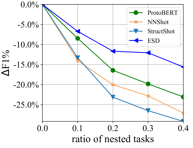
Sequence labeling tasks such as NER can have nested situations. For example, in the sentence “Isaac Newton studied at Cambridge University", where “Cambridge” is a location and “Cambridge University” is an organization. However, both FewNERD and SNIPS do not annotate nested examples. To explore the robustness of Esd on such a challenging but common situation, we construct FewNERD-nested, which has the same training tasks as FewNERD-INTRA, but different test tasks with a nested ratio . In FewNERD-nested, we sample each test task either from FewNERD or from GENIA Ohta et al. 2002 with the probability and , respectively, and all tasks sampled from GENIA are guaranteed to have the query with nested entities. We sample validation tasks with nested instances from ACE05 Walker et al. 2006 to tune , and in BSNMS. Please refer to the Appendix 8 for more details about FewNERD-nested. Figure 4 shows the results of Esd and several typical baselines in FewNERD-nested with different . When increases, Esd is more stable than previous methods, since Esd with BSNMS can easily extend to nested tagging cases without any extra training while previous methods are incapable of. In addition, we also compare different post-processing methods when . As shown in Table 4, the beam search method can not handle the nested situation, and thus it harms the performance. SoftNMS Shen et al. 2021 and BSNMS can both improve the model performance. However, when incorporating beam search into SoftNMS, the model can be more flexible and avoid some local optimal post-processing results achieved by SoftNMS (e.g., spans , and in Figure 3), and thus BSNMS outperforms SoftNMS 44 4 Esd is also more robust than baselines in the noisy situation. Please refer to Appendix 5 for details..
| Models | F1 |
|---|---|
| Esd (with BSNMS) | 31.25 |
| Esd (with SoftNMS) | 31.09 |
| Esd (with Beam Search) | 28.94 |
| Esd (without Post-processing) | 30.34 |
6.3 Model Efficiency
| Models | #Para. | Inference Time | |
|---|---|---|---|
| 1-shot | 5-shot | ||
| Esd | 112M | 8.53 ms | 18.47 ms |
| ProtoBERT | 110M | 3.13 ms | 5.27 ms |
| L-TapNet+CDT | 110M | 24.67 ms | 54.19 ms |
Compared with the token-level models, Esd needs to enumerate all spans within the length for a sentence. Therefore, the number of spans is approximately times that of tokens, which may bring extra computation overhead. To evaluate the efficiency of Esd, we compare the average inference time per task of Esd (including the BSNMS post-processing process), L-TapNet+CDT (the state-of-the-art token-level baseline model with the open codebase in the SNPIS) and ProtoBERT (an extremely simple token-level baseline). As shown in Table 5, with exactly the same hardware setting, in the domain “We” of SNIPS 1-shot setting, Esd (avg. ms per task) is nearly 3 times faster than L-TapNet+CDT (avg. ms per task). We see a similar tendency in the 5-shot setting. Although Esd (avg. and ms in 1- and 5-shot per task) is slower than ProtoBERT (avg. and ms), it outperforms ProtoBERT by and F1 scores in 1- and 5-shot settings (reported in Table 2) with a bearable latency. Besides the inference time, we also compare the parameter number of these models. As is shown, the added parameter scale (span enhancing and prototypical modules) is very small (2M) compared with the ProtoBERT and L-TapNet+CDT (110M). These results show that Esd has an acceptable efficiency.
| Models | F1 | Total | FP-Span | FP-Type |
|---|---|---|---|---|
| Esd | 59.29 | 9.4k | 72.8% | 27.2% |
| ProtoBERT | 38.83 | 30.4k | 86.7% | 13.3% |
| NNShot | 47.24 | 21.7k | 84.7% | 15.3% |
| StructShot | 51.88 | 14.5k | 80.0% | 20.0% |
6.4 Error Analysis
To further explore what types of errors the model makes in detail, we divide error of model prediction into categories, ‘FP-Span’ and ‘FP-Type’. As shown in Table 6, Esd outperforms baselines and has much less false positive prediction errors. ‘FP-Span’ is the major prediction error for all models, showing that it is hard to locate the right span boundary in FSSL for existing models. Therefore, we should pay more attention to the span recognition in the future work. However, compared with previous methods, Esd has less ratio of the ‘FP-span’ error. We think the reason is that our span-level matching framework with a series of span-related procedures has a better perception of the entity and slot spans than that of our baselines.
7 Conclusion
In this paper, we propose Esd, an enhanced span-based decomposition model for few-shot sequence labeling (FSSL). To overcome the drawbacks of previous token-level methods, Esd formulates FSSL as a span-level matching problem, and decomposes it into a series of span-related procedures, mainly including span representation, class prototype aggregation and span conflicts resolution for a better span matching. Extensive experiments show that Esd achieves the state-of-the-art performance on two popular few-shot sequence labeling benchmarks and that ESD is more robust than previous models in the noisy and nested situation.
Acknowledgements
The authors would like to thank the anonymous reviewers for their thoughtful and constructive comments. This paper is supported by the National Key Research and Development Program of China under Grant No. 2020AAA0106700, the National Science Foundation of China under Grant No.61936012 and 61876004, and NSFC project U19A2065.
References
- Athiwaratkun et al. (2020) Athiwaratkun, B.; Nogueira dos Santos, C.; Krone, J.; and Xiang, B. 2020. Augmented Natural Language for Generative Sequence Labeling. In Proceedings of the 2020 Conference on Empirical Methods in Natural Language Processing (EMNLP), 375–385. Online: Association for Computational Linguistics.
- Ba, Kiros, and Hinton (2016) Ba, J. L.; Kiros, J. R.; and Hinton, G. E. 2016. Layer normalization. arXiv preprint arXiv:1607.06450.
- Bodla et al. (2017) Bodla, N.; Singh, B.; Chellappa, R.; and Davis, L. S. 2017. Soft-NMS–improving object detection with one line of code. In Proceedings of the IEEE international conference on computer vision, 5561–5569.
- Coucke et al. (2018) Coucke, A.; Saade, A.; Ball, A.; Bluche, T.; Caulier, A.; Leroy, D.; Doumouro, C.; Gisselbrecht, T.; Caltagirone, F.; Lavril, T.; et al. 2018. Snips voice platform: an embedded spoken language understanding system for private-by-design voice interfaces. arXiv preprint arXiv:1805.10190.
- Cui et al. (2021) Cui, L.; Wu, Y.; Liu, J.; Yang, S.; and Zhang, Y. 2021. Template-Based Named Entity Recognition Using BART. In Findings of the Association for Computational Linguistics: ACL-IJCNLP 2021, 1835–1845. Online: Association for Computational Linguistics.
- Devlin et al. (2019) Devlin, J.; Chang, M.-W.; Lee, K.; and Toutanova, K. 2019. BERT: Pre-training of Deep Bidirectional Transformers for Language Understanding. In Proceedings of the 2019 Conference of the North American Chapter of the Association for Computational Linguistics: Human Language Technologies, Volume 1 (Long and Short Papers), 4171–4186. Minneapolis, Minnesota: Association for Computational Linguistics.
- Ding et al. (2021) Ding, N.; Xu, G.; Chen, Y.; Wang, X.; Han, X.; Xie, P.; Zheng, H.; and Liu, Z. 2021. Few-NERD: A Few-shot Named Entity Recognition Dataset. In Proceedings of the 59th Annual Meeting of the Association for Computational Linguistics and the 11th International Joint Conference on Natural Language Processing (Volume 1: Long Papers), 3198–3213. Online: Association for Computational Linguistics.
- Fritzler, Logacheva, and Kretov (2019a) Fritzler, A.; Logacheva, V.; and Kretov, M. 2019a. Few-shot classification in named entity recognition task. In Proceedings of the 34th ACM/SIGAPP Symposium on Applied Computing, 993–1000.
- Fritzler, Logacheva, and Kretov (2019b) Fritzler, A.; Logacheva, V.; and Kretov, M. 2019b. Few-shot classification in named entity recognition task. In Proceedings of the 34th ACM/SIGAPP Symposium on Applied Computing, 993–1000.
- Geng et al. (2019) Geng, R.; Li, B.; Li, Y.; Zhu, X.; Jian, P.; and Sun, J. 2019. Induction Networks for Few-Shot Text Classification. In Proceedings of the 2019 Conference on Empirical Methods in Natural Language Processing and the 9th International Joint Conference on Natural Language Processing (EMNLP-IJCNLP), 3904–3913. Hong Kong, China: Association for Computational Linguistics.
- Han et al. (2018) Han, X.; Zhu, H.; Yu, P.; Wang, Z.; Yao, Y.; Liu, Z.; and Sun, M. 2018. FewRel: A Large-Scale Supervised Few-Shot Relation Classification Dataset with State-of-the-Art Evaluation. In Proceedings of the 2018 Conference on Empirical Methods in Natural Language Processing, 4803–4809. Brussels, Belgium: Association for Computational Linguistics.
- He et al. (2016) He, K.; Zhang, X.; Ren, S.; and Sun, J. 2016. Deep residual learning for image recognition. In Proceedings of the IEEE conference on computer vision and pattern recognition, 770–778.
- Henderson and Vulić (2021) Henderson, M.; and Vulić, I. 2021. ConVEx: Data-Efficient and Few-Shot Slot Labeling. In Proceedings of the 2021 Conference of the North American Chapter of the Association for Computational Linguistics: Human Language Technologies, 3375–3389. Online: Association for Computational Linguistics.
- Hochreiter, Younger, and Conwell (2001a) Hochreiter, S.; Younger, A. S.; and Conwell, P. R. 2001a. Learning to learn using gradient descent. In International Conference on Artificial Neural Networks, 87–94. Springer.
- Hochreiter, Younger, and Conwell (2001b) Hochreiter, S.; Younger, A. S.; and Conwell, P. R. 2001b. Learning to learn using gradient descent. In International Conference on Artificial Neural Networks, 87–94. Springer.
- Hou et al. (2020) Hou, Y.; Che, W.; Lai, Y.; Zhou, Z.; Liu, Y.; Liu, H.; and Liu, T. 2020. Few-shot Slot Tagging with Collapsed Dependency Transfer and Label-enhanced Task-adaptive Projection Network. In Proceedings of the 58th Annual Meeting of the Association for Computational Linguistics, 1381–1393. Online: Association for Computational Linguistics.
- Kingma and Ba (2015) Kingma, D. P.; and Ba, J. 2015. Adam: A Method for Stochastic Optimization. CoRR, abs/1412.6980.
- Kulis et al. (2013) Kulis, B.; et al. 2013. Metric Learning: A Survey. Foundations and Trends® in Machine Learning, 5(4): 287–364.
- Lewis et al. (2020) Lewis, M.; Liu, Y.; Goyal, N.; Ghazvininejad, M.; Mohamed, A.; Levy, O.; Stoyanov, V.; and Zettlemoyer, L. 2020. BART: Denoising Sequence-to-Sequence Pre-training for Natural Language Generation, Translation, and Comprehension. In Proceedings of the 58th Annual Meeting of the Association for Computational Linguistics, 7871–7880.
- Ma et al. (2021) Ma, J.; Yan, Z.; Li, C.; and Zhang, Y. 2021. Frustratingly Simple Few-Shot Slot Tagging. In Findings of the Association for Computational Linguistics: ACL-IJCNLP 2021, 1028–1033. Online: Association for Computational Linguistics.
- Ohta et al. (2002) Ohta, T.; Tateisi, Y.; Kim, J.-D.; Mima, H.; and Tsujii, J. 2002. The GENIA corpus: An annotated research abstract corpus in molecular biology domain. In Proceedings of the human language technology conference, 73–77. Citeseer.
- Shen et al. (2021) Shen, Y.; Ma, X.; Tan, Z.; Zhang, S.; Wang, W.; and Lu, W. 2021. Locate and Label: A Two-stage Identifier for Nested Named Entity Recognition. In Proceedings of the 59th Annual Meeting of the Association for Computational Linguistics and the 11th International Joint Conference on Natural Language Processing (Volume 1: Long Papers), 2782–2794.
- Snell, Swersky, and Zemel (2017) Snell, J.; Swersky, K.; and Zemel, R. 2017. Prototypical networks for few-shot learning. In Proceedings of the 31st International Conference on Neural Information Processing Systems, 4080–4090.
- Srivastava et al. (2014) Srivastava, N.; Hinton, G.; Krizhevsky, A.; Sutskever, I.; and Salakhutdinov, R. 2014. Dropout: a simple way to prevent neural networks from overfitting. The journal of machine learning research, 15(1): 1929–1958.
- Vaswani et al. (2017) Vaswani, A.; Shazeer, N.; Parmar, N.; Uszkoreit, J.; Jones, L.; Gomez, A. N.; Kaiser, Ł.; and Polosukhin, I. 2017. Attention is all you need. In Advances in neural information processing systems, 5998–6008.
- Vinyals et al. (2016) Vinyals, O.; Blundell, C.; Lillicrap, T.; kavukcuoglu, k.; and Wierstra, D. 2016. Matching Networks for One Shot Learning. In Lee, D.; Sugiyama, M.; Luxburg, U.; Guyon, I.; and Garnett, R., eds., Advances in Neural Information Processing Systems, volume 29. Curran Associates, Inc.
- Walker et al. (2006) Walker, C.; Strassel, S.; Medero, J.; and Maeda, K. 2006. ACE 2005 multilingual training corpus. Linguistic Data Consortium, Philadelphia, 57: 45.
- Wang et al. (2021a) Wang, P.; Xun, R.; Liu, T.; Dai, D.; Chang, B.; and Sui, Z. 2021a. Behind the Scenes: An Exploration of Trigger Biases Problem in Few-Shot Event Classification. In Proceedings of the 30th ACM International Conference on Information & Knowledge Management, 1969–1978.
- Wang et al. (2021b) Wang, Y.; Mukherjee, S.; Chu, H.; Tu, Y.; Wu, M.; Gao, J.; and Awadallah, A. H. 2021b. Meta Self-training for Few-shot Neural Sequence Labeling. In Proceedings of the 27th ACM SIGKDD Conference on Knowledge Discovery & Data Mining, 1737–1747.
- Wang et al. (2020) Wang, Y.; Yao, Q.; Kwok, J. T.; and Ni, L. M. 2020. Generalizing from a few examples: A survey on few-shot learning. ACM Computing Surveys (CSUR), 53(3): 1–34.
- Yang and Katiyar (2020) Yang, Y.; and Katiyar, A. 2020. Simple and Effective Few-Shot Named Entity Recognition with Structured Nearest Neighbor Learning. In Proceedings of the 2020 Conference on Empirical Methods in Natural Language Processing (EMNLP), 6365–6375. Online: Association for Computational Linguistics.
- Yoon, Seo, and Moon (2019) Yoon, S. W.; Seo, J.; and Moon, J. 2019. Tapnet: Neural network augmented with task-adaptive projection for few-shot learning. In International Conference on Machine Learning, 7115–7123. PMLR.
- Yu et al. (2021) Yu, D.; He, L.; Zhang, Y.; Du, X.; Pasupat, P.; and Li, Q. 2021. Few-shot Intent Classification and Slot Filling with Retrieved Examples. In Proceedings of the 2021 Conference of the North American Chapter of the Association for Computational Linguistics: Human Language Technologies, 734–749. Online: Association for Computational Linguistics.
Appendix A Experiments
A.1 Baselines
We compare Esd with a variety of baselines as follows:
- •
TransferBERT Hou et al. 2020 is a fine-tuning based model, which is a direct application of BERT Devlin et al. 2019 to the few-shot sequence labeling.
- •
ConVEx Henderson and Vulić 2021 is a fine-tuning based model, which is first pre-trained on the Reddit corpus with the sequence labeling objective tasks and then fine-tuned on the source domain and target domain annotated data for final few shot sequence labelingm
- •
Ma2021 Ma et al. 2021 formulates sequence labeling as the machine reading comprehension problem, and proposes some questions to extract slots in the query sentence.
- •
ProtoBERT Fritzler, Logacheva, and Kretov 2019b predicts the query labels according to the similarity of BERT hidden states of support set and query tokens.
- •
Matching Net (MN)+BERT Hou et al. 2020 is similar to ProtoBERT. The only difference is that MN uses the matching network Vinyals et al. 2016 for token classification.
- •
L-TapNet-CDT Hou et al. 2020 utilizes the task-adaptive projection network Yoon, Seo, and Moon 2019, pair-wise embedding and collapsed dependency transfer mechanisms to do classification.
- •
NNShot Yang and Katiyar 2020 is similar to ProtoBERT, while it makes the prediction based on the nearest neighbor.
- •
StructShot Yang and Katiyar 2020 adopts an additional Viterbi decoder during the inference phase on top of NNShot.
- •
Retriever Yu et al. 2021 is a retrieval based method which does classification according to the most similar example in the support set.
A.2 Parameter Setting
In our implementation, we utilize BERT-base-uncased as our backbone encoder the same as Hou et al. 2020; Yu et al. 2021; Ding et al. 2021. We use Adam Kingma and Ba 2015 as our optimizer. In FewNERD, the learning rate is for BERT encoder and for other modules. In the 1-shot setting of SNIPS, for the domain “Mu”, the learning rate is for BERT encoder and for other modules. For the domain “Bo”, the learning rate is for BERT encoder and for other modules. For other settings of SNIPS, the learning rate is for BERT encoder and for other modules. We set the dropout ratio Srivastava et al. 2014 to . The dimension of span representation and the maximum span length is set to and , respectively. For BSNMS, the beam size is 5. Since these is no nested instances in FewNERD and SNIPS, we set the threshold to filter false positive spans to , the threshold to decay span scores to and the decay ratio to to force the refining results have no nested spans. We use the grid search to search our hyperparameters, and the scope of each hyperparameter are included in Table 7. We train our model on a single NVIDIA A40 GPU with 48GB memory.
| learning rate | [5e-5, 1e-4, 3e-4, 5e-4] |
|---|---|
| dropout | [0.1, 0.3, 0.5] |
| bert learning rate | [5e-6, 1e-5, 2e-5, 3e-5, 5e-5] |
| span dimension | [50, 100, 150, 200] |
| beam size | [1, 3, 5, 7] |
Appendix B FewNERD-nested
| [0.1, 0.2, 0.3, 0.4, 0.5, 0.6, 0.7, 0.8, 0.9] | |
| [0.1, 0.2, 0.3, 0.4, 0.5, 0.6, 0.7, 0.8, 0.9] | |
| [0.1, 0.2, 0.3, 0.4, 0.5, 0.6, 0.7, 0.8, 0.9] |
We construct our FewNERD-nested via ACE05 Walker et al. 2006, GENIA Ohta et al. 2002 and the origin FewNERD datasets. GENIA is a biological named entity recognition dataset, which contains 5 kinds of entities, ‘DNA’, ‘Protein’, ‘cell_type’, ‘RNA’ and ‘cell_line’, and all of these entity types are not included in the FewNERD. We partition the sentences in GENIA into two groups, and . consists of sentences with nested entities ( sentences in total), and consists of sentences without nested entities ( sentences in total). We utilize sentences in and to construct the query and support set of the GENIA task, respectively. Our FewNERD-nested contains 2000 5-way 510-shot test tasks in total, where percent tasks are from GENIA, and the remained tasks are from FewNERD-INTRA. We use ACE05 to construct the validation set. ACE05 is a widely used named entity recognition dataset, which contains coarse-grained entity types, ‘FAC’, ‘PER’, ‘LOC’, ‘VEH’, ‘GPE’, ‘GPE’, ‘WEA’ and ‘ORG’. The ‘LOC’, ‘PER’, ‘ORG’ and ‘FAC’ are not included in the training set of FewNERD-INTRA, and therefore we use them ( fine-grained entity types in total) and sample nested tasks as the validation dataset to tune the , and of BSNMS. The search scope is included in the Table 8. In this nested situation, we finally set the , and to , and respectively.
Appendix C Robustness in the Noisy Situation
FSSL methods tend to be seriously influenced by the noise in the support set, since they make the prediction based on only limited annotated examples. To explore the robustness of Esd in the noisy situation, we construct FewNERD-noise. In FewNERD-noise, we disturb each way shot FewNERD-INTRA task with a noisy ratio , which means there are nearly percent entities in the support set are mislabeled. As illustrated in the right part of Figure 5, with increasing, the performance of Esd drops less than baselines, which furthuer shows the superiority of our methods.
Appendix D A Detail Case Study of BSNMS
For span conflicts resolution, we propose a post-processing method BSNMS. A step by step demonstration of BSNMS is shown in Figure 6.
