Topological invariants in two-dimensional quasicrystals

We consider a doubly-periodic 2D Hamiltonian

where $V^{\lambda}(\mathbf{r})\,(\lambda=\alpha,\beta)$ is a periodic potential given by

and $\mathbf{b}_{1}^{\lambda},\mathbf{b}_{2}^{\lambda}$ are its primitive reciprocal lattice vectors. The real-space lattice vectors $\mathbf{a}_{1}^{\lambda},\mathbf{a}_{2}^{\lambda}$ are defined such that $\mathbf{a}^{\lambda}_{\mu}\cdot\mathbf{b}^{\lambda}_{\nu}=2\pi\delta_{\mu\nu}$. It is useful to introduce serial indexes to label the four reciprocal lattice vectors as

We claim that, when the spectrum has an energy gap, the electron density below an energy gap is quantized

Here $\nu_{ij}(i,j=1,2,3,4)$ are zone quantum numbers which characterize the gap, and $\langle i,j\rangle$ represents a pair of different indeces. $S^{*}_{ij}$ and $S_{ij}$ are defined by

where $(\cdots)_{z}$ represents the $z$-component perpendicular to the plane. $S^{*}_{ij}$ is a momentum space area spanned by two distinct reciprocal lattice vectors chosen from $\mathbf{b}_{1},\mathbf{b}_{2},\mathbf{b}_{3},\mathbf{b}_{4}$, and $S_{ij}$ is its real-space counterpart. We have six independent areas $S^{*}_{12},S^{*}_{13},S^{*}_{14},S^{*}_{23},S^{*}_{24},S^{*}_{34}$ as illustrated in Fig. 1(a), and we have $S^{*}_{ji}=-S^{*}_{ij}$ and $S^{*}_{ii}=0$ from the definition. Accordingly, we have six zone quantum numbers $\nu_{12},\nu_{13},\nu_{14},\nu_{23},\nu_{24},\nu_{34}$, and we define $\nu_{ji}=-\nu_{ij}$ and $\nu_{ii}=0$ for consistency. The areas $S^{*}_{ij}$ can be regarded as the projection of faces of four-dimensional hypercube onto the physical 2D plane.

The $S_{ij}$ is the area of the parallelogram formed by the wave surfaces of $e^{i\mathbf{b}_{i}\cdot\mathbf{r}}$ and $e^{i\mathbf{b}_{j}\cdot\mathbf{r}}$, as shown in Fig. 1(b). For later convenience, we define the lattice vectors

where $\mathbf{e}_{z}$ is the unit vector perpendicular to the 2D plane. $(\mathbf{a}^{ij}_{1},\mathbf{a}^{ij}_{2})$ is the primitive lattice vector set corresponding to $(\mathbf{b}^{ij}_{1},\mathbf{b}^{ij}_{2})\equiv(\mathbf{b}_{i},\mathbf{b}_{j})$ in the momentum space, and it spans the unit cell $S_{ij}=(\mathbf{a}^{ij}_{1}\times\mathbf{a}^{ij}_{2})_{z}$ as illustrated in Fig. 1(b). The lattice vectors of the potential $\alpha$ and $\beta$ are given by $\mathbf{a}^{\alpha}_{\mu}=\mathbf{a}^{12}_{\mu}$ and $\mathbf{a}^{\beta}_{\mu}=\mathbf{a}^{34}_{\mu}$.

In our previous workOka and Koshino 2021, we verified the relation Eq. (4) in a double-moiré system of graphene sandwiched by hexagonal boron nitride. There only four areas out of the six $S^{*}_{ij}$’s are independent due to the intrinsic 120^∘ rotational symmetry, and we identified the corresponding four zone quantum numbers for the energy gaps in the spectrum. The complete set of six integers can be obtained by allowing a slight deformation to break the symmetry. In the following, we demonstrate a full identification of the six characteristic integers in a double period system Eq. (1) with twisted double triangular potential. A similar calculation with twisted square potential is presented in Appendix B.

The twisted double triangular potential is given by

where $\mathbf{r}_{0}^{\lambda}$ is the origin of the potential $\lambda$. The reciprocal vectors of $\lambda=\alpha$ are given by

and those of $\beta$ are defined by

where $R(\theta)$ is a 2D rotation matrix of angle $\theta$. The corresponding primitive lattice vectors are

The potential profile is presented in Fig. 2, for (a) a single potential, (b) double potential with $\theta=7^{\circ}$ and (c) $\theta=30^{\circ}$. In the following, the potential amplitude (identical in $\alpha$ and $\beta$) is taken as $V_{0}=0.213\varepsilon_{0}$, where $\varepsilon_{0}=\hbar^{2}/(2ma^{2})$.

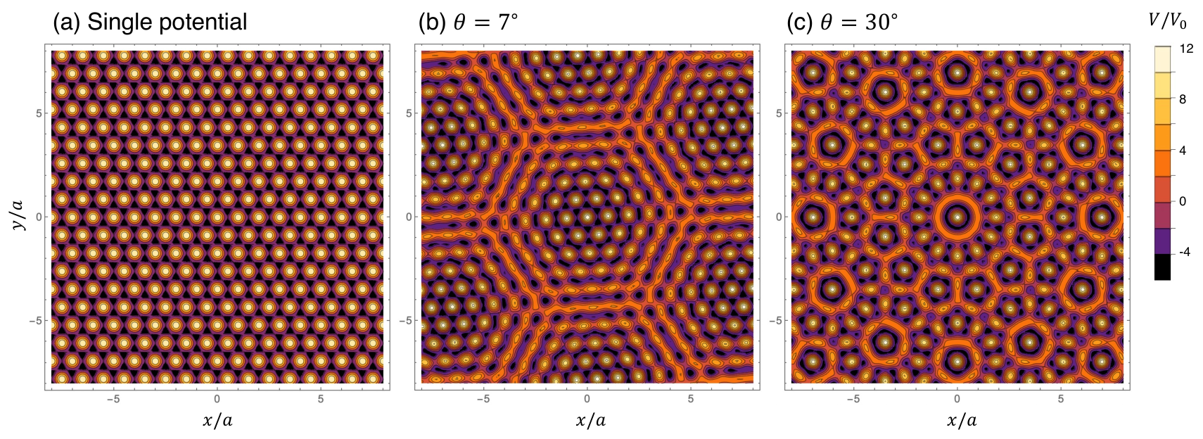
Generally, the potentials of $\alpha$ and $\beta$ do not have common period and hence the system does not have the global translational symmetry. Here we calculate the energy spectrum by using commensurate approximants Oka and Koshino 2021, which are obtained by slightly deforming the periodicity of $\alpha$ or $\beta$, so that the system has a finite super unit cell with an area $S_{\rm c}$. The detail of the commensurate approximant method is described in Appendix A. We prepare a series of commensurate approximants to mimic the continuous rotation of the twist angle between the two potentials, and calculate the energy bands and the density of states (DOS) for all the systems. For each approximant, we average the DOS over the relative translation $\Delta\mathbf{r}_{0}=\mathbf{r}_{0}^{\alpha}-\mathbf{r}_{0}^{\beta}$ to obtain a continuous spectrum as a function of the twist angle.

Figure 3(a) shows the density map of the DOS plotted against $\theta$ and energy, where the brighter color indicates larger DOS, and the dark blue region represents the gap. The array of bars in the upper part of the figure represents the commensurate approximants considered in the calculation. Figure 3(b) is the corresponding plot with vertical axis converted to the electron density, where dots represent energy gaps with the gap width indicated by the size.

For each energy gap, the zone quantum numbers $\nu_{ij}$ can be identified in the following manner. In a commensurate approximant, the momentum space area $S^{*}_{ij}$’s have the greatest common divisor $S^{*}_{\rm c}=(2\pi)^{2}/S_{\rm c}$, and hence they are expressed as $S^{*}_{ij}=s_{ij}S^{*}_{\rm c}$ with integers $s_{ij}$. Also, the electron density below a given band gap is quantized as $n_{e}=[S^{*}_{\rm c}/(2\pi)^{2}]r$, where $r$ in the number of the occupied Bloch subbands. Then, Eq. (4) becomes the Diophantine equation $r=\sum_{\langle i,j\rangle}\nu_{ij}s_{ij}$. By considering more than six commensurate approximants sharing the same energy gap, we have the Diophantine equations as many as the number of the approximants, and we finally obtain the integers $\nu_{ij}$ as a unique solution of the set of equations. It should be also noted that the original double triangular potential, Eq. (7), has constraints on $S^{*}_{ij}$’s such as $S^{*}_{12}=S^{*}_{34}$ and $S^{*}_{13}=S^{*}_{24}$ due to the high spatial symmetry, which prevents the full identification of $\nu_{ij}$’s. This problem is removed by including systems with the symmetry slightly broken in the set of commensurate approximants. The actual calculation of the zone quantum numbers using the commensurate approximants is presented in Appendix A.

In the bottom of Fig. 3, we present the zone quantum numbers $(\nu_{12},\nu_{13},\nu_{14},\nu_{23},\nu_{24},\nu_{34})$ identified for some major gaps labelled in Fig. 3(a) and (b). The series $M_{n}$ in the low twist angle regime is the moiré gaps, which has a form of

In this region, the system is governed by a long-range moiré pattern as seen in Fig. 2(b), and the discrete levels separated by $M_{n}$ can be viewed as the Bloch subbands of the moiré superlattice. The reciprocal lattice vectors for the moiré period are given by

and the area of the moiré Brillouin zone becomes

which corresponds to $(1,0,-1,1,0,1)$. Eq. (11) indicates that the momentum space area is quantized by $S^{*}_{\rm M}$.

In the large angle region $\theta\gg 1^{\circ}$, the long-wavelength picture is no longer valid and the system cannot be effectively captured by any single periodicity. At $\theta=30^{\circ}$, in particular, the system becomes a quasicrystal with 12-fold rotational symmetry Stampfli 1986; Ahn et al. 2018; Yao et al. 2018; Moon et al. 2019; Crosse and Moon 2021; Ha and Yang 2021, as shown in Fig. 2(c), Here we find that the zone quantum numbers always have the form,

The corresponding electronic density Eq. (4) is $n_{e}=(\sqrt{3}m+3n)/a^{2}$, indicating that there are two distinct units, $\sqrt{3}/a^{2}$ and $3/a^{2}$, to quantize the electronic spectrum.

The constraint on the zone quantum numbers Eq. (14) is explained as follows. If we define $\mathbf{b}^{\prime}_{i}\,(i=1,2,3,4)$ by the 30^∘-rotation of $\mathbf{b}_{i}$, we have a relation $(\mathbf{b}^{\prime}_{1},\mathbf{b}^{\prime}_{2},\mathbf{b}^{\prime}_{3},\mathbf{b}^{\prime}_{4})=(\mathbf{b}_{3},\mathbf{b}_{4},\mathbf{b}_{1}+\mathbf{b}_{2},-\mathbf{b}_{1})$. The associated areas $S^{*}_{ij}{{}^{\prime}}=(\mathbf{b}^{\prime}_{i}\times\mathbf{b}_{j}^{\prime})_{z}$ can be expressed by the old areas as $S^{*}_{12}{{}^{\prime}}=S^{*}_{34}$, $S^{*}_{13}{{}^{\prime}}=-S^{*}_{13}-S^{*}_{23}$, etc. When the system is invariant under the 30^∘-rotation, we should have $\sum_{\langle i,j\rangle}\nu_{ij}S^{*}_{ij}=\sum_{\langle i,j\rangle}\nu_{ij}S^{*}_{ij}{{}^{\prime}}$ with the identical $\nu_{ij}$. By using the relationship between $S^{*}_{ij}{{}^{\prime}}$ and $S^{*}_{ij}$, we obtain constraints for $\nu_{ij}$, and finially find Eq. (14).

Other gaps are just labelled as $A,B,C\cdots$ in Fig. 3. We see that the zone quantum numbers of any gaps definitely come in a form of $(m,n,r,n-r,n,m)$. This is explained by the coexistence of the 120^∘ rotational symmetry which requires the form of $(m,n,r,n-r,n,m^{\prime})$, and the reflection symmetry with respect to the in-plane axis between $\mathbf{b}_{1}$ and $\mathbf{b}_{3}$ which requires $(m,n,r,n-r,n^{\prime},m)$. The constraints on the zone quantum numbers are proved by a similar argument to the 12-fold case.

In our previous work Oka and Koshino 2021, we obtained only four zone quantum numbers in hBN/graphene/hBN systems because we only considered strictly 120^∘-symmetric commensurate approximants. There the unit areas have relationship $S^{*}_{24}=S^{*}_{13}$ and $S^{*}_{23}=-S^{*}_{13}-S^{*}_{14}$, so that $\sum_{\langle i,j\rangle}\nu_{ij}S^{*}_{ij}$ is reduced to $m_{1}S^{*}_{12}+m_{2}S^{*}_{34}+m_{3}S^{*}_{13}+m_{4}S^{*}_{14}$ with $(m_{1},m_{2},m_{3},m_{4})=(\nu_{12},\nu_{34},\nu_{13}-\nu_{23}+\nu_{24},\nu_{14}-\nu_{23})$, which are the four integers defined in Ref. Oka and Koshino 2021. Recalling that $\nu_{ij}$ must have the form $(m,n,r,n-r,n,m^{\prime})$ in 120^∘-symmetry, we can restore the complete six numbers $\nu_{ij}$ as $(m_{1},\frac{2m_{3}-m_{4}}{3},\frac{m_{3}+m_{4}}{3},\frac{m_{3}-2m_{4}}{3},\frac{2m_{3}-m_{4}}{3},m_{2})$. The numbers are found to be integers for all the gaps identified in Ref. Oka and Koshino 2021.

The area $\sum_{\langle i,j\rangle}\nu_{ij}S^{*}_{ij}$ can be associated with a geometric object in the momentum space referred to as the quasi Brillouin zone (qBZ). The boundary qBZ for a given gap is defined as a set of $k$-points on the original free-electron band, at which the gap starts to open in the infinitesimal potential limit. Oka and Koshino 2021 Generally, the qBZ is a polygon composed of multiple segments of Bragg planes, which are the perpendicular bisectors of composite reciprocal lattice vectors $\mathbf{G}=m_{1}\mathbf{b}_{1}+m_{2}\mathbf{b}_{2}+m_{3}\mathbf{b}_{3}+m_{4}\mathbf{b}_{4}$.

Let us consider the twisted triangular potential considered in the previous section. The qBZ for the moiré gap $M_{n}$ is found to be just $n$-th Brillouin zone defined by the moiré reciprocal vectors $\mathbf{G}^{\rm M}_{1}$ and $\mathbf{G}^{\rm M}_{2}$ [Eq. (12)]. In general twist angles, however, the qBZ does not coincide with any Brillouin zone of a periodic system. We show the qBZs of the gap $Q_{-1,1}$ and $Q_{-3,2}$ at $\theta=30^{\circ}$ in the leftmost panels of Fig. 4(a) and (b), respectively. The areas of these qBZs can be easily calculated by the decomposition illustrated in the right two panels. For instance, the area of the qBZ for gap $Q_{-1,1}$ [Fig. 4(a)] is expressed by three squares, $g_{1},g_{2},g_{3}$, and two hexagons $h_{1},h_{2}$ as $S^{*}(Q_{-1,1})=(g_{1}+g_{2}+g_{3})-(h_{1}+h_{2})$. The area $g_{1}$ is given by $g_{1}=(\mathbf{b}_{3}\times\mathbf{b}_{2})_{z}=-S^{*}_{23}$, and similarly we have $g_{2}=S^{*}_{14}+S^{*}_{24}$, $g_{3}=S^{*}_{13}+S^{*}_{14}$, $h_{1}=S^{*}_{12}$ and $h_{2}=S^{*}_{34}$. Finally we have $S^{*}(Q_{-1,1})=-S^{*}_{12}+S^{*}_{13}+2S^{*}_{14}-S^{*}_{23}+S^{*}_{24}-S^{*}_{34}$, which agrees with the zone quantum numbers $(-1,1,2,-1,1,-1)$ obtained in the previous section.

Similarly, the area of the qBZ for gap $Q_{-3,2}$ is expressed by $S^{*}(Q_{-3,2})=p_{1}+p_{2}+p_{3}-2q_{1}-q_{2}$ as shown Fig. 4(b). The area $p_{1}$ is the Wigner-Seitz cell in the reciprocal lattice of $\mathbf{b}_{1}$ and $\mathbf{b}_{3}$, and hence $p_{1}=S^{*}_{13}$. The $q_{1}$ (hexagon) and $q_{2}$ (six triangles) are the first and second Brillouin zones defined by the primitive vectors $\mathbf{b}_{1}-\mathbf{b}_{3}$ and $\mathbf{b}_{2}-\mathbf{b}_{4}$, and therefore $q_{1}=q_{2}=[(\mathbf{b}_{1}-\mathbf{b}_{3})\times(\mathbf{b}_{2}-\mathbf{b}_{4})]_{z}=S^{*}_{12}+S^{*}_{34}-S^{*}_{14}+S^{*}_{23}$. As a result, the area $S^{*}(Q_{-3,2})$ becomes $(-3,2,4,-2,2,-3)$.

At 30^∘, we have the symmetry constraints such as $g_{1}=g_{2}=g_{3}$ and one might think the decomposition of the qBZ area into $S^{*}_{ij}$’s is not unique. However, the area quantization with the same $\nu_{ij}$ strictly holds when the potential is deformed to break the symmetry, and this guarantees a uniqueness of the decomposition.

We first consider a doubly-periodic 1D Hamiltonian

where $V_{i}(x)=\sum_{m}V_{i,m}\,e^{imb_{i}x}(i=1,2)$ is a periodic potential with the period of $a_{i}=2\pi/b_{i}$. Now we consider a cyclic process where one of the periodic potential $V_{i}(x)$ is adiabatically translated by its period $a_{i}$, with the other fixed. The translated potential is expressed as

where an increase of $\phi_{i}$ from 0 to $2\pi$ gives a unit slide of $V_{i}(x)$ by distance $a_{i}$.

We define $\Delta P_{i}$ by the change of the electric polarization during a unit slide. In 1D, the $\Delta P_{i}$ has a dimension of the electronic density (number of electrons per a unit length) times length, which is dimensionless. Note that we exclude the electric charge $-e$ in the definition of the polarization. Here we claim the following: When the Fermi energy is in a gap, the polarization change per cycle, $\Delta P_{i}$, and the electron density below the gap, $n_{e}$, are related by

Eq. (17) can be proved by the following consideration. Let us consider an adiabatic process where the wavenumber $b_{i}$ is slightly changed to $b_{i}+\delta b_{i}$. As illustrated in Fig. 5, the corresponding change of $V_{i}(x)$ at a point far from the origin ($|x|\gg a_{i}$) can be viewed as a parallel translation of the fixed potential $V_{i}(x)$. Considering the phase factor $b_{i}x-\phi_{i}$ in Eq. (16), the change of $b_{i}$ to $b_{i}+\delta b_{i}$ can be absorbed to the change of $\phi_{i}$ by $\delta\phi_{i}=-\delta b_{i}\,x$, and this gives the phase shift in the effective translation at $x$. Since this process amounts to $n=\delta\phi_{i}/(2\pi)$ cycles of a unit translation, the number of electrons passing through the point $x$ is given by $n\Delta P_{i}=-\Delta P_{i}\delta b_{i}\,x/(2\pi)$. Due to the continuity of the electric charge, it must be equal to the change of the number of electrons in a region from 0 to $x$. This leads to a relation $-\Delta P_{i}\delta b_{i}\,x/(2\pi)=-x\delta n_{e}$, and we obtain Eq. (17).

In the doubly-periodic system given by Eq. (15), every gap in the spectrum is characterized by a pair of integers $m_{1}$ and $m_{2}$, such that the electron density below the gap is given by

By using Eq. (17), we conclude $\Delta P_{i}=m_{i}$, i.e., $m_{i}$ electrons passed through any cross section of the system. The integers $m_{1}$ and $m_{2}$ coincide with the first Chern numbers Thouless 1983; Niu 1986; Kraus et al. 2012; Fujimoto et al. 2020, as presented in Appendix A.

The same argument is available for a doubly-periodic 2D Hamiltonian, Eq. (1). We consider an adiabatic translation of the periodic potential $V^{\lambda}$ ($\lambda=\alpha$ or $\beta$) by $\mathbf{a}^{\lambda}_{\mu}$, and calculate the change of the electric polarization during the process. A parallel translation of $V^{\lambda}(\mathbf{r})$ is expressed as

where we used $\mathbf{a}^{\lambda}_{\mu}\cdot\mathbf{b}^{\lambda}_{\nu}=2\pi\delta_{\mu\nu}$. An increase of $\phi^{\lambda}_{\mu}$ from 0 to $2\pi$ gives a unit translation of the potential $V^{\lambda}$ by $\mathbf{a}^{\lambda}_{\mu}$.

The situation can be systematically described by a generalized Hamitonian $H=\mathbf{p}^{2}/(2m)+V$ with

The current double-period system corresponds to $N=4$, where $\mathbf{b}_{1},\cdots,\mathbf{b}_{4}$ are given by Eq. (3), and

We consider a cyclic process where $\phi_{i}$ of a certain $i$ is adiabatically increased from 0 to $2\pi$. When the Fermi energy is in a gap, we can show that the change of the electric polarization during the process is

which is the 2D version of Eq. (17). Now $\Delta\mathbf{P}_{i}$ has a dimension of the electronic density (number of electrons per a unit area) times length.

Eq. (22) is derived as follows. Let us consider the change of the potential $V(\mathbf{r})$ when $\mathbf{b}_{i}$ is changed to $\mathbf{b}_{i}+\delta\mathbf{b}_{i}$. In a similar manner to 1D case, the change at a point far from the origin ($|\mathbf{r}|\gg 2\pi/|\mathbf{b}_{i}|$) is equivalent to a parallel translation of $\delta\phi_{i}=-\delta\mathbf{b}_{i}\cdot\mathbf{r}$, noting the phase factor $\mathbf{b}_{i}\cdot\mathbf{r}-\phi_{i}$ in Eq. (20). This causes a polarization change by $\Delta\mathbf{P}_{i}\delta\phi_{i}/(2\pi)=\Delta\mathbf{P}_{i}(-\delta\mathbf{b}_{i}\cdot\mathbf{r})/(2\pi)$ at the point $\mathbf{r}$. The number of electrons passing through a line segment from $\mathbf{r}$ to $\mathbf{r}+d\mathbf{r}$ is given by

Now we consider a large closed path $C$ on the 2D plane, and let $N_{e}$ the number of electrons inside $C$. When $\mathbf{b}_{i}$ is changed to $\mathbf{b}_{i}+\delta\mathbf{b}_{i}$, the change of the $N_{e}$ is calculated by integrating Eq. (23) along the path, to obtain

where $S$ is the area of the region enclosed by $C$ and we used the relationship $\oint_{C}(d\mathbf{r}\times\mathbf{e}_{z})_{\mu}r_{\nu}=S\delta_{\mu\nu}$ in 2D. Since $n_{e}=N_{e}/S$, we end up with Eq. (22). Alternatively, Eq. (22) can also be derived in the infinitesimal potential limit, by integrating the Berry curvature on the boundary of the quasi Brillouin zone. The detailed argument is presented in Appendix C.

In a 2D doubly-periodic system, the electron density below an energy gap is quantized by Eq. (4), as argued in the previous section. By applying the formula Eq. (22) to Eq. (4), the charge pumping $\Delta\mathbf{P}_{i}$ is explicitly calculated as

where we used $S^{*}_{ij}=(\mathbf{b}_{i}\times\mathbf{b}_{j})\cdot\mathbf{e}_{z}=(\mathbf{b}_{j}\times\mathbf{e}_{z})\cdot\mathbf{b}_{i}$.

By using the real space lattice vectors Eq. (6), Eq. (25) can also be written as

The physical interpretation of Eq. (26) is as follows. Eq. (4) states that $\nu_{ij}$ electrons reside in each unit area of $S_{ij}$. When $\phi_{1}$ is changed from 0 to $2\pi$ (i.e., $V^{\alpha}$ is slid by $\mathbf{a}^{\alpha}_{1}$), for instance, the wave surface of $\mathbf{b}_{1}$ is moved by its single period, resulting in shifts of the unit areas $S_{12},S_{13},S_{14}$ by $\mathbf{a}^{12}_{1},\mathbf{a}^{13}_{1},\mathbf{a}^{14}_{1}$, respectively [See, Fig. 1(b)]. For each of $j=2,3,4$, the electron density of $\nu_{1j}/S_{1j}$ is transferred by $\mathbf{a}^{1j}_{1}$, resulting in a polarization change by $\Delta\mathbf{P}_{1}=\sum_{j=2,3,4}(\nu_{1j}/S_{1j})\mathbf{a}^{1j}_{1}$.

As an example, we consider the adiabatic pumping in the twisted triangular potential in Sec. II.2. For the moiré gap $M_{n}=n(1,0,-1,1,0,1)$ [Eq. (11)], Eq. (25) immediately leads to equations

where $\mathbf{L}^{\rm M}_{i}$ is the moiré lattice vector defined by

and we used Eq. (12). This indicates that, when the potential $\alpha(\beta)$ is slid by its unit vector $\mathbf{a}^{\alpha}_{\mu}(\mathbf{a}^{\beta}_{\mu})$, then $n$ electrons per the moiré unit cell are pumped by a moiré unit vector $n\mathbf{L}^{\rm M}_{\mu}(-n\mathbf{L}^{\rm M}_{\mu})$. The result coincides with the adiabatic moiré pumping in the previous works.Fujimoto et al. 2020; Zhang et al. 2020; Su and Lin 2020

The argument is also applicable to the quasicrystal gaps at $\theta=30^{\circ}$. Here the zone quantum numbers take the form $Q_{m,n}=(m,n,2n,-n,n,m)$ [Eq. (14)]. For $\Delta\mathbf{P}_{1}$, for instance, Eq. (25) gives

In the last equation, we used Eq. (10) and note that the electronic density [Eq. (4)] is $n_{e}=(\sqrt{3}m+3n)/L^{2}$ at $\theta=30^{\circ}$. By similar calculations, we have a set of equations independent of $m$ and $n$,

From the definition, $\Delta\mathbf{P}_{1}$ and $\Delta\mathbf{P}_{2}$ ($\Delta\mathbf{P}_{3}$ and $\Delta\mathbf{P}_{4}$) represent the polarization changes when the potential $\alpha$ ($\beta$) is translated by $\mathbf{a}^{\alpha}_{1}$ and $\mathbf{a}^{\alpha}_{2}$ ($\mathbf{a}^{\beta}_{1}$ and $\mathbf{a}^{\beta}_{2}$), respectively. Eq. (30) shows that, in any sliding processes, the transfer of the electric charge is always parallel to the potential sliding direction (regardless of which potential we move), and that the amount of the charge pumping is equivalent to the movement of the half of the total electric charge by the sliding vector.

References

- Ryu et al. (2010) S. Ryu, A. P. Schnyder, A. Furusaki, and A. W. Ludwig, New Journal of Physics 12, 065010 (2010).
- Qi and Zhang (2011) X.-L. Qi and S.-C. Zhang, Reviews of Modern Physics 83, 1057 (2011).
- Thouless et al. (1982) D. Thouless, M. Kohmoto, M. Nightingale, and M. Den Nijs, Phys. Rev. Lett. 49, 405 (1982).
- Kohmoto (1985) M. Kohmoto, Ann. Phys. 160, 343 (1985).
- Zoorob et al. (2000) M. Zoorob, M. Charlton, G. Parker, J. Baumberg, and M. Netti, Nature 404, 740 (2000).
- Kaliteevski et al. (2000) M. Kaliteevski, S. Brand, R. Abram, T. Krauss, R. D. Rue, and P. Millar, Nanotechnology 11, 274 (2000).
- Dyachenko et al. (2007) P. Dyachenko, Y. V. Miklyaev, and V. Dmitrienko, JETP Letters 86, 240 (2007).
- Krajčí and Hafner (2007) M. Krajčí and J. Hafner, Phys. Rev. B 75, 024116 (2007).
- Lang et al. (2012) L.-J. Lang, X. Cai, and S. Chen, Phys. Rev. Lett. 108, 220401 (2012).
- Mei et al. (2012) F. Mei, S.-L. Zhu, Z.-M. Zhang, C. Oh, and N. Goldman, Physical Review A 85, 013638 (2012).
- Kraus et al. (2012) Y. E. Kraus, Y. Lahini, Z. Ringel, M. Verbin, and O. Zilberberg, Phys. Rev. Lett. 109, 106402 (2012).
- Kraus and Zilberberg (2012) Y. E. Kraus and O. Zilberberg, Phys. Rev. Lett. 109, 116404 (2012).
- Satija and Naumis (2013) I. I. Satija and G. G. Naumis, Phys. Rev. B 88, 054204 (2013).
- Ganeshan et al. (2013) S. Ganeshan, K. Sun, and S. D. Sarma, Phys. Rev. Lett. 110, 180403 (2013).
- Verbin et al. (2013) M. Verbin, O. Zilberberg, Y. E. Kraus, Y. Lahini, and Y. Silberberg, Phys. Rev. Lett. 110, 076403 (2013).
- Verbin et al. (2015) M. Verbin, O. Zilberberg, Y. Lahini, Y. E. Kraus, and Y. Silberberg, Phys. Rev. B 91, 064201 (2015).
- Lohse et al. (2016) M. Lohse, C. Schweizer, O. Zilberberg, M. Aidelsburger, and I. Bloch, Nature Physics 12, 350 (2016).
- Marra and Nitta (2020) P. Marra and M. Nitta, Phys. Rev. Res. 2, 042035 (2020).
- Zilberberg (2021) O. Zilberberg, Optical Materials Express 11, 1143 (2021).
- Yoshii et al. (2021) M. Yoshii, S. Kitamura, and T. Morimoto, arXiv preprint arXiv:2105.05654 (2021).
- Kraus et al. (2013) Y. E. Kraus, Z. Ringel, and O. Zilberberg, Phys. Rev. Lett. 111, 226401 (2013).
- Tran et al. (2015) D.-T. Tran, A. Dauphin, N. Goldman, and P. Gaspard, Phys. Rev. B 91, 085125 (2015).
- Bandres et al. (2016) M. A. Bandres, M. C. Rechtsman, and M. Segev, Physical Review X 6, 011016 (2016).
- Cain et al. (2020) J. D. Cain, A. Azizi, M. Conrad, S. M. Griffin, and A. Zettl, Proceedings of the National Academy of Sciences 117, 26135 (2020).
- Rosa et al. (2021) M. I. Rosa, M. Ruzzene, and E. Prodan, Communications Physics 4, 1 (2021).
- Fujimoto et al. (2020) M. Fujimoto, H. Koschke, and M. Koshino, Phys. Rev. B 101, 041112 (2020).
- Zhang et al. (2020) Y. Zhang, Y. Gao, and D. Xiao, Phys. Rev. B 101, 041410 (2020).
- Su and Lin (2020) Y. Su and S.-Z. Lin, Phys. Rev. B 101, 041113 (2020).
- Thouless (1983) D. Thouless, Phys. Rev. B 27, 6083 (1983).
- Niu (1986) Q. Niu, Phys. Rev. B 34, 5093 (1986).
- Lopes dos Santos et al. (2007) J. Lopes dos Santos, N. Peres, and A. Castro Neto, Phys. Rev. Lett. 99, 256802 (2007).
- Mele (2010) E. Mele, Phys. Rev. B 81, 161405 (2010).
- Trambly de Laissardière et al. (2010) G. Trambly de Laissardière, D. Mayou, and L. Magaud, Nano Lett. 10, 804 (2010).
- Shallcross et al. (2010) S. Shallcross, S. Sharma, E. Kandelaki, and O. Pankratov, Phys. Rev. B 81, 165105 (2010).
- Morell et al. (2010) E. Morell, J. Correa, P. Vargas, M. Pacheco, and Z. Barticevic, Phys. Rev. B 82, 121407 (2010).
- Bistritzer and MacDonald (2011) R. Bistritzer and A. MacDonald, Proc. Natl. Acad. Sci. 108, 12233 (2011).
- Moon and Koshino (2012) P. Moon and M. Koshino, Phys. Rev. B 85, 195458 (2012).
- de Laissardiere et al. (2012) G. T. de Laissardiere, D. Mayou, and L. Magaud, Phys. Rev. B 86, 125413 (2012).
- Dean et al. (2010) C. Dean, A. Young, I. Meric, C. Lee, L. Wang, S. Sorgenfrei, K. Watanabe, T. Taniguchi, P. Kim, K. Shepard, and J. Hone, Nat. Nanotechnol. 5, 722 (2010).
- Ponomarenko et al. (2013) L. A. Ponomarenko, R. V. Gorbachev, G. L. Yu, D. C. Elias, R. Jalil, A. A. Patel, A. Mishchenko, A. S. Mayorov, C. R. Woods, J. R. Wallbank, M. Mucha-Kruczynski, B. A. Piot, M. Potemski, I. V. Grigorieva, K. S. Novoselov, F. Guinea, V. I. Fal’ko, and A. K. Geim, Nature 497, 594 (2013).
- Hunt et al. (2013) B. Hunt, J. Sanchez-Yamagishi, A. Young, M. Yankowitz, B. LeRoy, K. Watanabe, T. Taniguchi, P. Moon, M. Koshino, P. Jarillo-Herrero, and R. Ashoori, Science 340, 1427 (2013).
- Cao et al. (2018a) Y. Cao, V. Fatemi, S. Fang, K. Watanabe, T. Taniguchi, E. Kaxiras, and P. Jarillo-Herrero, Nature 556, 43 (2018a).
- Cao et al. (2018b) Y. Cao, V. Fatemi, A. Demir, S. Fang, S. L. Tomarken, J. Y. Luo, J. D. Sanchez-Yamagishi, K. Watanabe, T. Taniguchi, E. Kaxiras, R. C. Ashoori, and P. Jarillo-Herrero, Nature 556, 80 (2018b).
- Zou et al. (2018) L. Zou, H. C. Po, A. Vishwanath, and T. Senthil, Phys. Rev. B 98, 085435 (2018).
- Koshino et al. (2018) M. Koshino, N. F. Yuan, T. Koretsune, M. Ochi, K. Kuroki, and L. Fu, Phys. Rev. X 8, 031087 (2018).
- Balents et al. (2020) L. Balents, C. R. Dean, D. K. Efetov, and A. F. Young, Nature Physics 16, 725 (2020).
- Stampfli (1986) P. Stampfli, Helv. Phys. Acta 59, 1260 (1986).
- Ahn et al. (2018) S. J. Ahn, P. Moon, T.-H. Kim, H.-W. Kim, H.-C. Shin, E. H. Kim, H. W. Cha, S.-J. Kahng, P. Kim, M. Koshino, et al., Science 361, 782 (2018).
- Yao et al. (2018) W. Yao, E. Wang, C. Bao, Y. Zhang, K. Zhang, K. Bao, C. K. Chan, C. Chen, J. Avila, M. C. Asensio, et al., Proceedings of the National Academy of Sciences 115, 6928 (2018).
- Moon et al. (2019) P. Moon, M. Koshino, and Y.-W. Son, Phys. Rev. B 99, 165430 (2019).
- Crosse and Moon (2021) J. A. Crosse and P. Moon, Phys. Rev. B 103, 045408 (2021).
- Ha and Yang (2021) H. Ha and B.-J. Yang, arXiv preprint arXiv:2103.08851 (2021).
- Oka and Koshino (2021) H. Oka and M. Koshino, Phys. Rev. B 104, 035306 (2021).
- Finney et al. (2019) N. R. Finney, M. Yankowitz, L. Muraleetharan, K. Watanabe, T. Taniguchi, C. R. Dean, and J. Hone, Nature nanotechnology 14, 1029 (2019).
- Wang et al. (2019a) L. Wang, S. Zihlmann, M.-H. Liu, P. Makk, K. Watanabe, T. Taniguchi, A. Baumgartner, and C. Schönenberger, Nano letters 19, 2371 (2019a).
- Wang et al. (2019b) Z. Wang, Y. B. Wang, J. Yin, E. Tóvári, Y. Yang, L. Lin, M. Holwill, J. Birkbeck, D. Perello, S. Xu, et al., Science advances 5, eaay8897 (2019b).
- Yang et al. (2020) Y. Yang, J. Li, J. Yin, S. Xu, C. Mullan, T. Taniguchi, K. Watanabe, A. K. Geim, K. S. Novoselov, and A. Mishchenko, arXiv preprint arXiv:2010.03798 (2020).
- Onodera et al. (2020) M. Onodera, K. Kinoshita, R. Moriya, S. Masubuchi, K. Watanabe, T. Taniguchi, and T. Machida, Nano letters 20, 4566 (2020).
- Kuiri et al. (2021) M. Kuiri, S. K. Srivastav, S. Ray, K. Watanabe, T. Taniguchi, T. Das, and A. Das, Phys. Rev. B 103, 115419 (2021).
- Andelkovic et al. (2020) M. Andelkovic, S. P. Milovanovic, L. Covaci, and F. M. Peeters, Nano letters 20, 979 (2020).
- Leconte and Jung (2020) N. Leconte and J. Jung, 2D Materials 7, 031005 (2020).
- Qi et al. (2008) X.-L. Qi, T. L. Hughes, and S.-C. Zhang, Phys. Rev. B 78, 195424 (2008).
- Price et al. (2015) H. M. Price, O. Zilberberg, T. Ozawa, I. Carusotto, and N. Goldman, Phys. Rev. Lett. 115, 195303 (2015).
- Price et al. (2016) H. M. Price, O. Zilberberg, T. Ozawa, I. Carusotto, and N. Goldman, Phys. Rev. B 93, 245113 (2016).
- Lohse et al. (2018) M. Lohse, C. Schweizer, H. M. Price, O. Zilberberg, and I. Bloch, Nature 553, 55 (2018).
- Zilberberg et al. (2018) O. Zilberberg, S. Huang, J. Guglielmon, M. Wang, K. P. Chen, Y. E. Kraus, and M. C. Rechtsman, Nature 553, 59 (2018).
- Lu et al. (2018) L. Lu, H. Gao, and Z. Wang, Nat. Commun. 9, 1 (2018).
- Penrose (1974) R. Penrose, Bull. Inst. Math. Appl. 10, 266 (1974).
- Walter and Deloudi (2009) S. Walter and S. Deloudi, Crystallography of quasicrystals: concepts, methods and structures, Vol. 126 (Springer Science & Business Media, 2009).
- Hatsugai and Fukui (2016) Y. Hatsugai and T. Fukui, Phys. Rev. B 94, 041102 (2016).
- Fujimoto and Koshino (2021) M. Fujimoto and M. Koshino, Phys. Rev. B 103, 155410 (2021).