Geometric decomposition of entropy production in out-of-equilibrium systems
Abstract
Two qualitatively different ways of driving a physical system out of equilibrium, time-dependent and non-conservative forcing, are reflected by the decomposition of the system’s entropy production into excess and housekeeping parts. We show that the difference between these two types of driving gives rise to a geometric formulation in terms of two orthogonal contributions to the currents in the system. This geometric picture in a natural way leads to variational expressions for both the excess and housekeeping entropy, which allow calculating both contributions independently from the trajectory data of the system. We demonstrate this by calculating the excess and housekeeping entropy of a particle in a time-dependent, tilted periodic potential.
A particle system in equilibrium with its environment may be driven out of equilibrium in two qualitatively different ways: Either, we vary the parameters of the system according to a time-dependent protocol. In this case, if we imagine suspending the protocol at any given instant, the system will relax back to the equilibrium state corresponding to the instantaneous values of the parameters. Alternatively, we can also apply a time-independent, nonconservative force to the system. In this case, even though the system will eventually relax to a steady state, this steady state will be out-of-equilibrium due to persistent currents in the system. In both cases, the degree to which the system is out of equilibrium at any given time is characterized by a positive rate of entropy production .
Generically, a system may be driven by time-dependent and nonconservative forces at the same time. Then, a natural question is whether the effects of both types of driving on the entropy production can be separated Landauer 1978; Oono and Paniconi 1998; Hatano and Sasa 2001; Ruelle 2003; Komatsu et al. 2008; Bertini et al. 2013; Maes and Netočnỳ 2014. For Brownian particles, we may decompose the entropy production rate into two nonnegative contributions, called excess and housekeeping entropy production rate, respectively Hatano and Sasa 2001; Maes and Netočnỳ 2014. Here, is positive whenever the state of the system depends on time and vanishes in a steady state. By contrast, is positive whenever the system is driven by a nonconservative force and vanishes if only conservative forces are acting on the system. Somewhat surprisingly, this decomposition is not unique; specifically, the decompositions due to Hatano and Sasa Hatano and Sasa 2001 and due to Maes and Netočnỳ Maes and Netočnỳ 2014 both satisfy the above properties but are generally distinct.
Such a decomposition of entropy production is very appealing from a theoretical point of view, since it allows deriving extended forms of fundamental results like the fluctuation theorem Hatano and Sasa 2001 and the Clausius heat theorem Maes and Netočnỳ 2014. However, the excess and housekeeping entropy are generally difficult to obtain directly from experimental and numerical data. The reason is that, in the case of Ref. Hatano and Sasa 2001, we need to determine the instantaneous steady state of the system, whereas for Ref. Maes and Netočnỳ 2014, we need to construct a conservative force with the same time evolution, both of which typically require an analytic description of the system. This issue has been addressed in Ref. Komatsu et al. 2008 by defining the excess entropy in terms of heat currents, with the downside that the result only holds in linear response.
In this Letter, our first main result is a geometric formalism for decomposing the entropy production rate into orthogonal gradient and nongradient fields, which describes both the Hatano-Sasa (HS) and the Maes-Netočnỳ (MN) decomposition. This unifying formalism also provides the relation between the two decompositions: the MN decomposition is the one that minimizes the housekeeping part, which is thus always less than in the HS decomposition. Our second main result is that, in the case of the MN decomposition, the geometric formalism provides variational expressions that can be used to calculate or estimate the excess and housekeeping entropy from experimental or numerical trajectory data. This implies that the latter decomposition can be used to identify the contributions due to time-dependent and nonconservative driving in practical applications, while retaining its favorable theoretical properties. We demonstrate our results using a particle in a time-dependent tilted periodic potential.
Geometric decomposition of entropy production. The probability density of a system of Brownian particles with coordinates evolves according to the Fokker-Planck equation
| (1a) | ||||
| (1b) | ||||
Here the time-dependent force contains interactions between the particles as well as conservative and nonconservative external forces, is the particle mobility and is the temperature of the environment. In the following, we will assume natural boundary conditions, that is, that the probability density and its derivatives vanish as , where denotes the Euclidean norm of . The local mean velocity is a vector field that describes the local average flows in the system. Importantly, it also determines the rate of entropy production,
| (2) |
where we defined the inner product between two vector fields (assuming and are such that it exists)
| (3) |
We then decompose the flows into two orthogonal components,
| (4) |
For any such decomposition of the flows, the Pythagorean theorem immediately yields a decomposition of the entropy production rate into two positive parts,
| (5) |
The decomposition Eq. (4) is not unique; the goal is to find a physically meaningful decomposition. We observe that, from the definition of the local mean velocity Eq. (1), it can be written as a gradient field whenever the forces acting in the system are conservative , where is the potential. Since in this case, the housekeeping entropy production should vanish, we make the ansatz
| (6) |
that is, we decompose the local mean velocity into a gradient field and the remainder. In the HS decomposition Hatano and Sasa 2001, the central idea is to consider the instantaneous steady state of the system, which is attained when fixing the force to its instantaneous value and letting the system relax to the corresponding steady state (which we assume to exist). This steady state is characterized by a steady-state local mean velocity which satisfies the steady state equation . Further, we have , which suggests choosing . By explicit computation (see the Supplemental Material sup), it can be verified that this choice indeed satisfies Eq. (4). We thus obtain the HS decomposition
| (7) |
Another possibility is to demand that should be orthogonal to all gradient fields, i. e., for all . As we discuss below, this condition results in the MN decomposition Maes and Netočnỳ 2014
| (8) |
where is the unique gradient field that satisfies . Thus, both the HS and MN decomposition can be viewed as decompositions of the local mean velocity into a gradient field and an orthogonal remainder, which is our first main result. This the geometrical intuition underlying the MN decomposition is illustrated in Fig. 1(a).
Variational expressions. Since the vector fields and in Eq. (4) are orthogonal, they define a decomposition of the space of all local mean velocities into two orthogonal subspaces and . Conversely, can be viewed as the orthogonal projection of into the subspace . Then, we have two variational expressions for the square of the “length” of ,
| (9a) | ||||
| (9b) | ||||
The first expression follows by noting for all and then considering the equality condition of the Cauchy-Schwarz inequality . The second expression can be confirmed by writing, for ,
| (10) |
which is minimized for . Eq. (9) allows us to consider the inner product either as a maximization over the subspace or a minimization over the subspace . For the MN decomposition, this is illustrated graphically in Fig. 1(b): The orthogonal projection can be obtained by either maximizing the overlap between and some gradient field, or minimizing the length of the complement.
If is chosen as the space of gradient fields, then we immediately have
| (11) |
On the other hand, the orthogonality condition explicitly reads from Eq. (3)
| (12) |
after integrating by parts. Since the condition should hold for all , this implies . Comparing this to Eq. (1), the space can thus be characterized as all vector fields that can be added to without altering the time evolution of . Since this is equivalent to changing the force , Eq. (11) implies a minimization of the entropy production rate with respect to the force, while keeping the time evolution of fixed. This is exactly the minimum entropy production principle of Ref. Maes and Netočnỳ 2014 and, thus, Eq. (8) is indeed the same as the MN decomposition. In view of Eq. (9), the appealing feature of the MN decomposition is that one of the two subspaces has a simple mathematical characterization as the space of gradient fields, which allows us to write
| (13) | ||||
| (14) |
From Eq. (14), we see that we may obtain an upper bound on the MN housekeeping entropy production rate by choosing an arbitrary gradient gradient field. For the particular choice , the right-hand side is equal to the HS housekeeping entropy production rate, so that we obtain the relation
| (15) |
Thus, while the HS and MN decomposition are generally distinct, there exists a definite relation between the two. We remark that, in principle, expressions similar to Eq. (13) and Eq. (14) can be obtained for the HS decomposition; however, the structure of the orthogonal spaces is more complicated, and the resulting variational expressions are not convenient for practical applications.
Excess entropy and Wasserstein distance. In the following, we will focus on the MN decomposition and drop the superscript MN from now on. Since the MN excess entropy production is the minimal entropy for a given time evolution of the probability density, we can also write is as
| (16) |
where, on the right hand side, we minimize over the vector field under the constraint that it satisfies the continuity equation Eq. (1a). This expression closely resembles the Benamou-Brenier Benamou and Brenier 2000 formula from optimal transport theory. Since the latter gives an equivalent expression of the Wasserstein distance between two probability densities Villani 2008, we obtain the identification between the MN excess entropy production rate and the Wasserstein distance (for more details, see sup),
| (17) |
In Refs. Aurell et al. 2011; Aurell et al. 2012; Dechant and Sakurai 2019, it was found that the minimum entropy production associated with changing the probability density from an initial state to a finial state can be expressed in terms of the Wasserstein distance between the two states. Eq. (17) generalizes this result to the case where, instead of the initial and final state, the time evolution of the probability density is fixed Nakazato and Ito 2021.
Excess and housekeeping entropy from trajectory data. In order to obtain expressions more suited to applications, we use the explicit form of the inner product Eq. (3),
| (18) |
where we integrated by parts and used Eq. (1). Here denotes an average with respect to . This allows us to write the excess entropy production rate as
| (19) |
The right-hand side can be evaluated by only considering scalar observables that are a function of the position of the Brownian particles. The maximization can then be readily performed using a suitable parameterization of . The maximizer of Eq. (19) yields the optimal local mean velocity up to a constant, . This is the flow field that yields the same time evolution as Eq. (1) while minimizing the entropy production rate. In contrast to directly minimizing the entropy production rate, Eq. (19) does not require any additional constraints. Instead of maximizing the right-hand side of Eq. (19) with respect to , we can also choose an arbitrary scalar function and obtain a lower bound. We remark that Eq. (13) is closely related to the short-time version of the thermodynamic uncertainty relation Manikandan et al. 2020; Otsubo et al. 2020; Van Vu et al. 2020: If the maximization is taken over all vector fields, then the result is the total entropy production rate; by restricting the maximization to gradient fields, the result is the excess entropy production.
In order to obtain a similar expression for the housekeeping entropy, we write the force acting on the system as , where is a nonconservative force. Since in Eq. (14), the infimum is taken over all gradient fields, we may absorb the gradient terms in the local mean velocity into and write
| (20) |
In many physical settings, the nonconservative force is an externally applied driving force and its functional form is therefore known. In such cases, we can evaluate Eq. (20) by considering only scalar observables that depend on the position of the particles. We stress that Eq. (20) does not depend explicitly on the potential , which generally includes interactions between particles and is therefore often not known precisely in practice. Without minimizing, an arbitrary choice of yields an upper bound on the housekeeping entropy production rate. One meaningful such choice is , which yields the upper bound
| (21) |
Thus, the housekeeping entropy production rate is bounded by the variance of the nonconservative force. In summary, the variational expressions Eq. (19) and Eq. (20) allow us to determine both the excess and the housekeeping entropy production rate from given trajectory data, which is our second main result.
Demonstration. As an explicit demonstration of our previous results, we study the motion of a Brownian particle in a time-dependent periodic potential , which is driven by a constant bias ,
| (22) |
Such a situation is common in experimental systems to study the dynamics of colloidal particles Speck and Seifert 2007; Evstigneev et al. 2008. For simplicity, we modulate the potential in a time-periodic manner, . For long times, the probability density is then periodic in both space and time, . We perform numerical simulations of Eq. (22), from which we obtain a set of trajectories, which we then use to compute the excess and housekeeping entropy production rate according to Eq. (19) and Eq. (20). Note that for periodic boundary conditions, only forces that can be written as the gradient of a periodic scalar function are conservative. Thus, we parameterize the scalar functions and as
| (23) |
with and evaluate Eq. (19) and Eq. (20). Then, we numerically optimize resulting expressions with respect to the parameters and using Mathematica’s NMaximize and NMinimize routines. We stress that determining and in this manner requires only the trajectories and the value of the bias . As a concrete example, we choose the space-time periodic potential
| (24) |
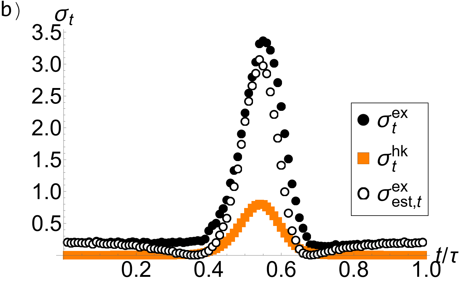
which corresponds to a sine-shaped potential with a time-dependent component of amplitude and period . The resulting excess and housekeeping entropy rates averaged over one period are shown as a function of the driving period in Fig. 2a). First, we note that the sum precisely reproduces the entropy production rate, calculated according to the stochastic thermodynamics result Sekimoto 2010; Seifert 2012. As expected, the entropy is dominated by the excess contribution for fast driving, while for slow driving, the housekeeping part from the constant bias is dominant. For the present example, the housekeeping entropy rate is almost independent of the driving speed, reflecting that, to a good approximation, the time-dependent probability density depends on only via a rescaling of time. However, unlike in a steady state, the housekeeping entropy production rate strongly depends on time, as can be seen from Fig. 2b): The main contribution to the entropy production stems from times , where the total depth of the potential is minimal.

Discussion. In this work, we decomposed the entropy production using the geometric formalism of orthogonal projections. While the extension to diffusion matrices and multiplicative noise is possible, a more serious challenge is to find a similar interpretation for other classes of stochastic dynamics, notably underdamped Langevin and Markov jump dynamics Maes and Netočnỳ 2007. In both cases, it has been recently shown that entropy production is bounded from below by an appropriately defined Wasserstein distance Dechant and Sakurai 2019; Van Vu and Hasegawa 2021; Dechant 2021; in light of Eq. (17), we may thus speculate that the latter can be identified with an excess entropy similar to the MN decomposition also in these cases.
Generally, variational principles and geometry are often intimately connected, be it in classical mechanics Arnol’d 2013 or optimal transport theory Villani 2008. The geometric decomposition Eq. (6) implies the variational formulas Eq. (9) for the individual contributions to the entropy production rate. Recently, the partial entropy production of subsystems was also shown to follow from a variational principle Ito et al. 2020, based on the projection theorem of information geometry Amari 2016. While the maximum entropy principle of equilibrium statistical mechanics Jaynes 1982 can be recast in a geometric formalism involving an orthogonal decomposition of the underlying space Pavon and Ferrante 2013, the above results suggest that a viable for obtaining minimum entropy production principles Jaynes 1980 may be starting from a suitable geometric decomposition of the space.
Acknowledgements.
S. I. thanks Muka Nakazato, Masafumi Oizumi, Shin-ichi Amari and Kohei Yoshimura for fruitful discussions. S. I. is supported by JSPS KAKENHI (Grant No. 19H05796, 21H01560), JST Presto (Grant No. JPMJPR18M2) and UTEC-UTokyo FSI Research Grant Program. S. S. is supported by JSPS KAKENHI (Grant No. 17H01148, 19H05795, and 20K20425).Supplemental Material
.1 Orthogonality for the Hatano-Sasa decomposition
In the Hatano-Sasa decomposition of the entropy production rate, the local mean velocity is decomposed using the local mean velocity of the instantaneous steady state
| (S25) |
where satisfies
| (S26) | ||||
Comparing this to the definition of the local mean velocity (see Eq. (1) of the main text),
| (S27) |
we see that the difference is a gradient field,
| (S28) |
so that this decomposition is of the form (see Eq. (6) of the main text)
| (S29) |
Next, we calculate the inner product (defined in Eq. (3) of the main text) between and
| (S30) |
We introduce a factor and note that to obtain
| (S31) |
Using the divergence theorem and Eq. (S26), we find
| (S32) |
Thus, the two terms in Eq. (S25) are indeed orthogonal with respect to the inner product defined by .
.2 Excess entropy and Wasserstein distance
As discussed in the main text and in Ref. Maes and Netočnỳ 2014, the Maes-Netočnỳ excess entropy production is the minimum entropy production rate associated with the time evolution of the probability density . In Refs. Aurell et al. 2011; Aurell et al. 2012; Dechant and Sakurai 2019 it was found that the minimum entropy production associated with changing the probability density from an initial state to a finial state can be expressed in terms of the Wasserstein distance Villani 2008 between the two states
| (S33) |
where is the duration of the process. For an arbitrary process connecting the two states, the right-hand side is a lower bound on the entropy production . For a given time evolution connecting to , we can imagine minimizing the entropy production rate at any instant of time. Since the result is still a process connecting the same initial and final state, we immediately have
| (S34) |
where is the excess entropy production. This implies that the right-hand side of Eq. (S33) can estimate only the excess part of the entropy production. Further, in Ref. Nakazato and Ito 2021 it was shown that
| (S35) |
with equality when the dynamics is driven by a conservative force. Since the excess entropy production rate represents a process with the same time evolution and driven by a conservative force, we immediately have the identification
| (S36) |
which shows that Eq. (S34) becomes an equality in the short-time limit. Thus, we can identify the Maes-Netočnỳ excess entropy production rate with the infinitesimal Wasserstein distance along the time evolution of the probability density.
References
- Landauer (1978) R. Landauer, far from equilibrium, Phys. Rev. A 18, 255 (1978).
- Oono and Paniconi (1998) Y. Oono and M. Paniconi, Steady state thermodynamics, Prog. Theor. Phys. Suppl. 130, 29 (1998).
- Hatano and Sasa (2001) T. Hatano and S.-i. Sasa, Steady-state thermodynamics of Langevin systems, Phys. Rev. Lett. 86, 3463 (2001).
- Ruelle (2003) D. P. Ruelle, Extending the definition of entropy to nonequilibrium steady states, Proc. Natl. Acad. Sci. 100, 3054 (2003).
- Komatsu et al. (2008) T. S. Komatsu, N. Nakagawa, S.-i. Sasa, and H. Tasaki, Steady-state thermodynamics for heat conduction: microscopic derivation, Phys. Rev. Lett. 100, 230602 (2008).
- Bertini et al. (2013) L. Bertini, D. Gabrielli, G. Jona-Lasinio, and C. Landim, Clausius inequality and optimality of quasistatic transformations for nonequilibrium stationary states, Phys. Rev. Lett. 110, 020601 (2013).
- Maes and Netočnỳ (2014) C. Maes and K. Netočnỳ, A nonequilibrium extension of the Clausius heat theorem, J. Stat. Phys. 154, 188 (2014).
- (8) See the Supplemental Material, which contains additional technical details as well as the derivation of the relation between the excess entropy and Wasserstein distance.
- Benamou and Brenier (2000) J.-D. Benamou and Y. Brenier, A computational fluid mechanics solution to the Monge-Kantorovich mass transfer problem, Numer. Math. 84, 375 (2000).
- Villani (2008) C. Villani, Optimal Transport: Old and New, Grundlehren der mathematischen Wissenschaften (Springer Berlin Heidelberg, 2008).
- Aurell et al. (2011) E. Aurell, C. Mejía-Monasterio, and P. Muratore-Ginanneschi, Optimal protocols and optimal transport in stochastic thermodynamics, Phys. Rev. Lett. 106, 250601 (2011).
- Aurell et al. (2012) E. Aurell, K. Gawedzki, C. Mejía-Monasterio, R. Mohayaee, and P. Muratore-Ginanneschi, Refined second law of thermodynamics for fast random processes, J. Stat. Phys. 147, 487 (2012).
- Dechant and Sakurai (2019) A. Dechant and Y. Sakurai, Thermodynamic interpretation of wasserstein distance, arXiv preprint arXiv:1912.08405 (2019).
- Nakazato and Ito (2021) M. Nakazato and S. Ito, Geometrical aspects of entropy production in stochastic thermodynamics based on wasserstein distance, Phys. Rev. Research 3, 043093 (2021).
- Manikandan et al. (2020) S. K. Manikandan, D. Gupta, and S. Krishnamurthy, Inferring entropy production from short experiments, Phys. Rev. Lett. 124, 120603 (2020).
- Otsubo et al. (2020) S. Otsubo, S. Ito, A. Dechant, and T. Sagawa, Estimating entropy production by machine learning of short-time fluctuating currents, Phys. Rev. E 101, 062106 (2020).
- Van Vu et al. (2020) T. Van Vu, V. T. Vo, and Y. Hasegawa, Entropy production estimation with optimal current, Phys. Rev. E 101, 042138 (2020).
- Speck and Seifert (2007) T. Speck and U. Seifert, The jarzynski relation, fluctuation theorems, and stochastic thermodynamics for non-markovian processes, J. Stat. Mech. Theory E. 2007, L09002 (2007).
- Evstigneev et al. (2008) M. Evstigneev, O. Zvyagolskaya, S. Bleil, R. Eichhorn, C. Bechinger, and P. Reimann, Diffusion of colloidal particles in a tilted periodic potential: Theory versus experiment, Phys. Rev. E 77, 041107 (2008).
- Sekimoto (2010) K. Sekimoto, Stochastic Energetics, Lecture Notes in Physics (Springer Berlin Heidelberg, 2010).
- Seifert (2012) U. Seifert, Stochastic thermodynamics, fluctuation theorems and molecular machines, Rep. Prog. Phys. 75, 126001 (2012).
- Maes and Netočnỳ (2007) C. Maes and K. Netočnỳ, Minimum entropy production principle from a dynamical fluctuation law, J. Math. Phys. 48, 053306 (2007).
- Van Vu and Hasegawa (2021) T. Van Vu and Y. Hasegawa, Geometrical bounds of the irreversibility in markovian systems, Phys. Rev. Lett. 126, 010601 (2021).
- Dechant (2021) A. Dechant, Minimum entropy production, detailed balance and Wasserstein distance for continuous-time Markov processes (2021), arXiv:2110.01141 [cond-mat.stat-mech] .
- Arnol’d (2013) V. I. Arnol’d, Mathematical methods of classical mechanics, Vol. 60 (Springer Science & Business Media, 2013).
- Ito et al. (2020) S. Ito, M. Oizumi, and S.-i. Amari, Unified framework for the entropy production and the stochastic interaction based on information geometry, Phys. Rev. Research 2, 033048 (2020).
- Amari (2016) S.-i. Amari, Information geometry and its applications, Vol. 194 (Springer, 2016).
- Jaynes (1982) E. T. Jaynes, On the rationale of maximum-entropy methods, Proc. IEEE 70, 939 (1982).
- Pavon and Ferrante (2013) M. Pavon and A. Ferrante, On the geometry of maximum entropy problems, SIAM review 55, 415 (2013).
- Jaynes (1980) E. T. Jaynes, The minimum entropy production principle, Annu. Rev. Phys. Chem. 31, 579 (1980).