Relevance of Shear Transformations in the Relaxation of Supercooled Liquids
Abstract
While deeply supercooled liquids exhibit divergent viscosity and increasingly heterogeneous dynamics as the temperature drops, their structure shows only seemingly marginal changes. Understanding the nature of relaxation processes in this dramatic slowdown is key for understanding the glass transition. Here, we show by atomistic simulations that the heterogeneous dynamics of glass-forming liquids strongly correlate with the local residual plastic strengths along soft directions computed in the initial inherent structures. The correlation increases with decreasing temperature and is maximum in the vicinity of the relaxation time. For the lowest temperature investigated, this maximum is comparable with the best values from the literature dealing with the structure-property relationship. However, the nonlinear probe of the local shear resistance in soft directions provides here a real-space picture of relaxation processes. Our detection method of thermal rearrangements allows us to investigate the first passage time statistics and to study the scaling between the activation energy barriers and the residual plastic strengths. These results shed new light on the nature of relaxations of glassy systems by emphasizing the analogy between the thermal relaxations in viscous liquids and the plastic shear transformation in amorphous solids.
When cooled fast enough, most substances avoid crystallization and form a glass Cavagna 2009. Before reaching the glass transition, they are trapped in a supercooled liquid metastable state, with a diverging relaxation time as the temperature is lowered, and show complex dynamics Keys et al. 2011 marked by the presence of dynamical heterogeneities Ediger 2000. A fundamental problem in condensed matter that has remained unsolved so far is that it is extremely difficult to identify any structural signature associated with this dramatic change in dynamics. Still, a clear link between structure and dynamics is implied by the increased sensitivity of the dynamics to the initial structural conditions as the temperature decreases Widmer-Cooper et al. 2004. Recent major advances rely on the identification of the so-called locally favored structures Malins et al. 2013 and indicate the necessity of employing a locally coarse-grained description of the structure Berthier and Jack 2007; Tong and Tanaka 2018; Boattini et al. 2021. Remarkable progress has also been achieved using multibody order parameters Tong and Tanaka 2019; Tong and Tanaka 2020 or advanced machine learning methods Schoenholz et al. 2016; Bapst et al. 2020; Boattini et al. 2020; Paret et al. 2020; Sharma et al. 2022.
Although these different approaches have established an unprecedented link between local dynamics and structure, most rely upon scalar quantities, i.e., they disregard the orientation dependencies. Furthermore, the underlying mechanisms of the relaxation processes have remained elusive. Contrasting results have been reported in the literature showing that thermally activated excitations could take the form of single atomic jumps Vollmayr-Lee 2004, stringlike motions Donati et al. 1999; Vogel et al. 2004; Ji et al. 2022 or local shears Widmer-Cooper and Harrowell 2009. In all cases, the spatial structure of the relaxations tends to localize with decreasing temperature Coslovich et al. 2019; Shimada et al. 2021.
A promising approach to understanding the relaxation of supercooled liquids consists of reversing the problem by considering highly viscous liquids as flowing solids Dyre 2006. The rationale behind this approach relies upon the description of liquids from a potential energy landscape point of view Goldstein 1969; Debenedetti and Stillinger 2001. In this picture, for sufficiently low temperatures, the system spends most of its time vibrating around potential energy minima before quickly jumping to other minima. A succession of Inherent States (ISs) can thus describe the dynamics Doliwa and Heuer 2003. More than a mere simplification, this solidlike description has enabled the understanding of key aspects of glass-forming liquids from a mechanical description of their ISs Heuer 2008; Del Gado et al. 2008. Perturbative approaches based on soft vibrational modes have been linked to irreversible rearrangements Widmer-Cooper et al. 2008, a non-Arrhenian characteristic energy scale has been identified in fragile liquids Lerner and Bouchbinder 2018; Kapteijns et al. 2021 and the presence of long-range anisotropic stress correlations explained Lemaître 2014. All of these studies point to the importance of soft localized excitations. However, a direct link between relaxations in liquids and the local nonlinear plastic rearrangements of ISs remains to be established Li et al. 2022.
This Letter aims to demonstrate how local soft directions in the initial ISs account for the local relaxation rates of the parent supercooled liquids. For this, we rely on a local shear test (LST) numerical method providing access to the local residual plastic strength Patinet et al. 2016. This structural indicator has proved to be very helpful in athermal amorphous solids for capturing the barrier dependencies to preparation Barbot et al. 2018, shear banding Barbot et al. 2020, anisotropy Patinet et al. 2020 and to predict plastic activity Richard et al. 2020.
We analyze molecular dynamics (MD) simulations of supercooled liquids equilibrated at different temperatures from which temporal series of ISs are generated. A strong connection is established between the local residual plastic strength computed in the initial ISs along the weakest shear direction and the local dynamics. The maximum correlation is found around the system relaxation time and increases as the temperature decreases. Additionally, a remarkable correlation is established between the core displacement fields of athermal plastic and thermal rearrangements, respectively observed in LST and MD. The thermal excitations are shown to be more frequent in the softest shear directions, thus providing a real-space picture of the relaxation processes. Local relaxation locations and first passage times are detected using the linear response of underlying ISs. This method allows us to investigate the scaling relation between the energy barriers and the residual plastic strengths Johnson and Samwer 2005; Maloney and Lacks 2006; Fan et al. 2014.
Simulation methods. - The systems under study are two-dimensional binary mixtures Barbot et al. 2018. A sample contains atoms interacting via Lennard-Jones (LJ) potentials vanishing at a cutoff distance (see Supplemental Material SM). MD simulations are performed in the NVT ensemble in square boxes equipped with periodic boundary conditions. In the following, all observables are expressed in LJ units.
The results that we analyze are taken from independent samples simulated at three temperatures , , and , respectively located around the onset temperature, the mode-coupling crossover and in a regime below which the MD equilibrium sampling starts to be numerically untractable. The systems are equilibrated such that the potential energy is stationary over a time . The relaxation time is estimated from the self-intermediate scattering function using the first neighbor cage-relative (CR) displacements Shiba et al. 2016 such that , with the average atomic distance. Going from high to low temperature, the relaxation time diverges: , and .
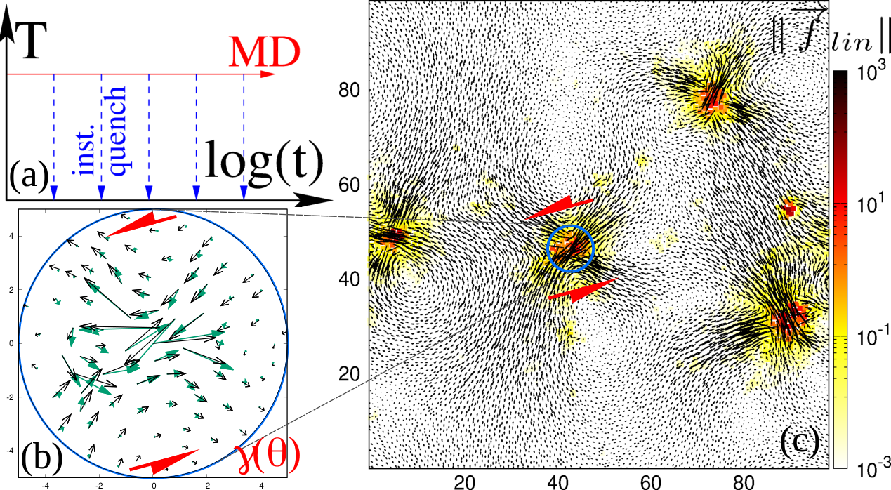
ISs are generated along the MD run by instantaneously quenching configurations at logarithmic increasing time intervals [see Fig. 1(a)]. MD configurations are relaxed with balanced forces on each atom using a conjugate gradient algorithm. The kinematics of supercooled liquids can then be greatly simplified and reduced to a sequence of ISs by removing thermal vibrations. Studying the inherent dynamics allows us to focus on the influence of the underlying potential energy landscape Doliwa and Heuer 2003; Vogel et al. 2004; Heuer 2008.
In Fig. 1(b) and 1(c), we respectively show typical core and long-range thermal rearrangement displacement fields between two ISs. We observe a strong localization of around rearrangements. The displacement fields in the core of these localized excitations show a wide range of complex behaviors, from single atomic jumps to more spread and intricate patterns. However, a striking feature of the long-range is the presence of quadrupolar symmetries Lemaître 2014; Nishikawa et al. 2022 around the rearrangements as shown in Fig. 1(c). This is a characteristic feature of Eshelby’s plastic shear transformations, more commonly discussed in the context of amorphous plasticity Tanguy et al. 2006; Maloney and Lemaître 2006. This is a strong hint of the local shear character of thermally activated events in supercooled liquids Widmer-Cooper and Harrowell 2009. We also observe exchange events between atoms, without long-range elastic response, that remain in the minority SM.

Local shear test method. – To study the influence of mechanical properties of the initial structure on the dynamics, we perform LSTs Barbot et al. 2018 in the ISs at time . The method consists of shearing a local circular inclusion at position by applying affine pure shear boundary conditions to the surrounding atoms in a shear direction (see Fig. 1). The atoms inside are deformed via the quasistatic athermal method Maloney and Lemaître 2004 and can relax nonaffinely. The inclusion is loaded until a drop in local stress indicates the first plastic instability SM. We extract two quantities from the LSTs: the residual plastic strength and the plastic instability displacement field corresponding to the stress drop . These two observables are sampled with inclusion radii , at positions on a regular square grid of lattice parameter and in directions , every .
The values of statistically increase when decreasing the parent temperature SM, showing that this observable is able to capture the energy barrier’s increase with the decrease of the temperature, i.e. the liquid fragility Cavagna 2009; Kallel et al. 2010. In the following, we show that also determines most of the spatial fluctuations of the dynamics. While isotropy prevails in a statistical sense, the values of the directional strongly depend on the local shear directions and positions, thus reflecting the disordered character of the amorphous structure Barbot et al. 2018; Patinet et al. 2020. For liquids, the thermally induced excitations are statistically isotropic, so one would expect the onset of local relaxations to be dominated by the residual strengths along the weakest directions: . We therefore consider in the following these values in local softest directions and compare them with the system dynamics.
Dynamical observables. – To emphasize the influence of the structure, we perform MD simulations in the isoconfigurational ensemble Widmer-Cooper et al. 2004. In this ensemble, multiple independent runs are started using the same initial configuration, but the particles’ momenta are drawn from a Maxwell-Boltzmann distribution for each run. For each starting configuration, replica are simulated. The dynamic propensity is computed as a function of time by averaging the CR square displacement over the isoconfigurational ensemble of each atom Li et al. 2022. The propensity is finally coarse grained on the same regular grid as with a coarse-graining length equal to to compare these quantities on an equal footing. A map is reported in Fig. 2(a). It shows the characteristic dynamical heterogeneities Ediger 2000; Keys et al. 2011, with some broadening due to the coarse-graining procedure SM.
Although valuable, the information provided by results from an accumulation of rearrangements which cannot be analyzed separately. To address this issue, and detect the positions of rearrangements, we compute the linear force response between two ISs Lemaître 2014. From time to , where is the Hessian matrix evaluated in the IS at . We then consider the norm on each atom. If the atom motions correspond to the linear response of the system, is equal to zero because of mechanical balance. On the other hand, large are expected in the highly distorted, nonlinear, regions. This is what is observed in Fig. 1(c) where features large values at the cores of the thermal rearrangements while vanishing in the rest of the system. Although it requires working in ISs, several advantages of this method should be stressed. First, it is sensitive and spans several orders of magnitude between rearranged and elastically disturbed regions. Second, it erases the long-range linear elastic fields induced by rearrangements. Finally, it is not affected by rigid body motions.

We choose to consider as being rearranged the atoms for which , with SM. This allows us to define the local first passage time when this criterion is fulfilled for the first time during a trajectory starting from . For each time lag and for each isolated clusters of atoms with , the locations of the successive isolated thermal rearrangements are extracted from the positions of the atom carrying the largest . For each event, we also record the local maximum shear strain direction denoted from the local strain field Barbot et al. 2020. The number of events between two ISs increases with temperature and time window . The isoconfigurational averages of first passage times reported in Fig. 2(b) show again characteristic dynamical heterogeneities of supercooled liquids. The comparison of and shows striking similarities, meaning that parts of the short and long dynamics are correlated. In our view, however, provides an easier grasp of the initial local structural relaxation timescale compared with accumulated mean square displacements.
Correlation between dynamics and . – In Fig. 2, we compare the , and maps. Their similarity is remarkable. The softer the region, the faster its relaxation. As an example, the first isolated thermal events of a particular MD trajectory are reported in Fig 2c. They are systematically located in the softest areas. More quantitatively, to analyze the correlation between the rearrangement locations and the initial structure, we report in Fig. 3(a) the ranking correlation defined in Ref. Patinet et al. 2016 from the cumulative distribution function as where is the value of the field at where the thermal event takes place at . shows that the correlation is larger for the smallest temperatures and decreases over time, the system losing the memory of its original structure.
The Pearson correlation between the fields and is plotted as a function of time in Fig. 3(b). We observe that the correlation increases with time as the successive thermal relaxations accumulate, with a peak around . The correlation with the field is quantitatively close to that with SM. Remarkably, for the lowest temperature, we find a maximum correlation comparable to the maximum correlations found in literature such those obtained from machine learning Bapst et al. 2020; Boattini et al. 2020 and to the order parameter proposed in Ref. Tong and Tanaka 2019 (see Supplemental Material for a detailed comparison SM).

We go one step further and directly evaluate the correlation between and in the core regions of the first passage rearrangements. An example of such a comparison reported in Fig. 1(b) shows a striking agreement between the two fields. The correlation is calculated as the maximum over all LST directions of the dot product of the normalized vector fields and . Figure 3(c) shows correlation as a function of the orientation deviation . We observe a maximum when the thermal rearrangements are aligned with the softest directions, i.e. for . This maximum of correlation obtained on the full set of first passage thermal rearrangements reaches significantly high values with a median in the range while the mean lies a bit below in the range . This slight contrast reflects the fact that the distribution presents a peak close to 1, i.e. to quasi-identity between plastic and thermal events.
In addition to barrier heights, this result shows that the mechanisms of shear transformation and thermal relaxation share remarkable similarities. Besides the correlation, we report in Fig. 3(d) the probability distribution showing a clear peak around , which means that thermal rearrangement’s shear directions are more frequent in the vicinity of softest directions. This last observation is fully consistent with the interpretation of fast dynamics in the soft regions of ISs, whose hop frequencies are dominated by the weakest directions.
Scaling of energy barriers. – Once the correlation is established, we discuss now the quantitative relation between and . The effective activation energy is fitted assuming an Arrhenius law in the form with a prefactor and the energy barrier. The actual temperature dependence of the characteristic time is disregarded, and is used as a tunable parameter allowing one to collapse the results obtained at different temperatures. As shown in Fig. 4, we find a scaling of barriers as a function of the residual plastic strengths . If an exponent , compatible with the catastrophe theory Johnson and Samwer 2005; Maloney and Lacks 2006; Fan et al. 2014, can not be totally ruled out, the fit of our data gives . Interestingly, this result is in quantitative agreement with , a scaling that can be deduced from the relations and found in Ref. Kapteijns et al. 2020 [see Eqs. (35) and (37) therein] where is the frequency of the nonlinear quasilocalized excitations in quiescent glasses. It is to our knowledge the first time it has been obtained locally at finite temperature. This scaling relation can be understood as a reflection of the sensitivity of the lowest barriers to stress, which is identified here in the local softest directions by the LST.
Concluding remarks and perspectives. – In this Letter, we have established a strong correlation between residual plastic strengths in the softest direction of the initial IS and the dynamics of glass-forming liquids. The softer the zones of ISs, the faster the local region of liquids. An advantage of this picture over purely geometrical approaches is that it provides a simple real-space interpretation of relaxations as localized shear events in soft directions. Among the possible transition paths, a local shear allows particles to escape from their cage for moderate long-range elastic energy cost. As a local stress, is a naturally coarse-grained quantity Berthier and Jack 2007; Tong and Tanaka 2018. Shear transformations thus involve cooperative motions in the spirit of an Adam-Gibbs-style scenario Cavagna 2009; Berthier 2021 and long-range generated elastic interactions providing intuitive support to the dynamic facilitation picture Chacko et al. 2021; Hasyim and Mandadapu 2021; Scalliet et al. 2021. By pointing to the central role played by the mechanics of ISs at low temperatures, these results are useful for understanding the onset of rigidity and the theoretical description of the glass transition.
Acknowledgements.
The present work was initiated during the PhD thesis of the late Matthias Lerbinger. A.B., S.P. and D.V. dedicate this article to his memory.References
- Cavagna (2009) A. Cavagna, Phys. Rep, 476, 51 (2009).
- Keys et al. (2011) A. S. Keys, L. O. Hedges, J. P. Garrahan, S. C. Glotzer, and D. Chandler, Phys. Rev. X, 1, 021013 (2011).
- Ediger (2000) M. D. Ediger, Annu. Rev. Phys. Chem, 51, 99 (2000).
- Widmer-Cooper et al. (2004) A. Widmer-Cooper, P. Harrowell, and H. Fynewever, Phys. Rev. Lett., 93, 135701 (2004).
- Malins et al. (2013) A. Malins, J. Eggers, C. P. Royall, S. R. Williams, and H. Tanaka, J. Chem. Phys., 138, 12A535 (2013).
- Berthier and Jack (2007) L. Berthier and R. L. Jack, Phys. Rev. E, 76, 041509 (2007).
- Tong and Tanaka (2018) H. Tong and H. Tanaka, Phys. Rev. X, 8, 011041 (2018).
- Boattini et al. (2021) E. Boattini, F. Smallenburg, and L. Filion, Phys. Rev. Lett., 127, 088007 (2021).
- Tong and Tanaka (2019) H. Tong and H. Tanaka, Nat. Commun., 10, 5596 (2019).
- Tong and Tanaka (2020) H. Tong and H. Tanaka, Phys. Rev. Lett., 124, 225501 (2020).
- Schoenholz et al. (2016) S. S. Schoenholz, E. D. Cubuk, D. M. Sussman, E. Kaxiras, and A. J. Liu, Nat. Phys, 12, 469 (2016).
- Bapst et al. (2020) V. Bapst, T. Keck, A. Grabska-Barwińska, C. Donner, E. D. Cubuk, S. S. Schoenholz, A. Obika, A. W. R. Nelson, T. Back, D. Hassabis, and P. Kohli, Nat. Phys, 16, 448 (2020).
- Boattini et al. (2020) E. Boattini, S. Marín-Aguilar, S. Mitra, G. Foffi, F. Smallenburg, and L. Filion, Nat. Commun., 11, 5479 (2020).
- Paret et al. (2020) J. Paret, R. L. Jack, and D. Coslovich, J. Chem. Phys., 152, 144502 (2020).
- Sharma et al. (2022) M. Sharma, M. K. Nandi, and S. M. Bhattacharyya, Phys. Rev. E, 105, 044604 (2022).
- Vollmayr-Lee (2004) K. Vollmayr-Lee, J. Chem. Phys., 121, 4781 (2004).
- Donati et al. (1999) C. Donati, S. C. Glotzer, P. H. Poole, W. Kob, and S. J. Plimpton, Phys. Rev. E, 60, 3107 (1999).
- Vogel et al. (2004) M. Vogel, B. Doliwa, A. Heuer, and S. C. Glotzer, J. Chem. Phys., 120, 4404 (2004).
- Ji et al. (2022) W. Ji, T. W. J. de Geus, E. Agoritsas, and M. Wyart, Phys. Rev. E, 105, 044601 (2022).
- Widmer-Cooper and Harrowell (2009) A. Widmer-Cooper and P. Harrowell, Phys. Rev. E, 80, 061501 (2009).
- Coslovich et al. (2019) D. Coslovich, A. Ninarello, and L. Berthier, SciPost Phys., 7, 77 (2019).
- Shimada et al. (2021) M. Shimada, D. Coslovich, H. Mizuno, and A. Ikeda, SciPost Phys., 10, 001 (2021).
- Dyre (2006) J. C. Dyre, Rev. Mod. Phys., 78, 953 (2006).
- Goldstein (1969) M. Goldstein, J. Chem. Phys., 51, 3728 (1969).
- Debenedetti and Stillinger (2001) P. G. Debenedetti and F. H. Stillinger, Nature (London), 410, 259 (2001).
- Doliwa and Heuer (2003) B. Doliwa and A. Heuer, Phys. Rev. Lett., 91, 235501 (2003).
- Heuer (2008) A. Heuer, J. Phys. Condens. Matter, 20, 373101 (2008).
- Del Gado et al. (2008) E. Del Gado, P. Ilg, M. Kröger, and H. C. Öttinger, Phys. Rev. Lett., 101, 095501 (2008).
- Widmer-Cooper et al. (2008) A. Widmer-Cooper, H. Perry, P. Harrowell, and D. R. Reichman, Nat. Phys, 4, 711 (2008).
- Lerner and Bouchbinder (2018) E. Lerner and E. Bouchbinder, J. Chem. Phys., 148, 214502 (2018).
- Kapteijns et al. (2021) G. Kapteijns, D. Richard, E. Bouchbinder, T. B. Schrøder, J. C. Dyre, and E. Lerner, J. Chem. Phys., 155, 074502 (2021).
- Lemaître (2014) A. Lemaître, Phys. Rev. Lett., 113, 245702 (2014).
- Li et al. (2022) Y.-W. Li, Y. Yao, and M. P. Ciamarra, Phys. Rev. Lett., 128, 258001 (2022).
- Patinet et al. (2016) S. Patinet, D. Vandembroucq, and M. L. Falk, Phys. Rev. Lett., 117, 045501 (2016).
- Barbot et al. (2018) A. Barbot, M. Lerbinger, A. Hernandez-Garcia, R. García-García, M. L. Falk, D. Vandembroucq, and S. Patinet, Phys. Rev. E, 97, 033001 (2018).
- Barbot et al. (2020) A. Barbot, M. Lerbinger, A. Lemaître, D. Vandembroucq, and S. Patinet, Phys. Rev. E, 101, 033001 (2020).
- Patinet et al. (2020) S. Patinet, A. Barbot, M. Lerbinger, D. Vandembroucq, and A. Lemaître, Phys. Rev. Lett., 124, 205503 (2020).
- Richard et al. (2020) D. Richard, M. Ozawa, S. Patinet, E. Stanifer, B. Shang, S. A. Ridout, B. Xu, G. Zhang, P. K. Morse, J.-L. Barrat, L. Berthier, M. L. Falk, P. Guan, A. J. Liu, K. Martens, S. Sastry, D. Vandembroucq, E. Lerner, and M. L. Manning, Phys. Rev. Mater., 4, 113609 (2020).
- Johnson and Samwer (2005) W. L. Johnson and K. Samwer, Phys. Rev. Lett., 95, 195501 (2005).
- Maloney and Lacks (2006) C. E. Maloney and D. J. Lacks, Phys. Rev. E, 73, 061106 (2006).
- Fan et al. (2014) Y. Fan, T. Iwashita, and T. Egami, Nat. Commun., 5, 5083 (2014).
- (42) See below Supplemental Material for details about the system, the local shear test, the propensity coarse-graining, the thermal relaxation detection, and the exchange events, which includes Refs. Falk and Langer 1998; Lemaître and Caroli 2007.
- Shiba et al. (2016) H. Shiba, Y. Yamada, T. Kawasaki, and K. Kim, Phys. Rev. Lett., 117, 245701 (2016).
- Nishikawa et al. (2022) Y. Nishikawa, M. Ozawa, A. Ikeda, P. Chaudhuri, and L. Berthier, Phys. Rev. X, 12, 021001 (2022).
- Tanguy et al. (2006) A. Tanguy, F. Leonforte, and J.-L. Barrat, Eur. Phys. J. E, 20, 355 (2006).
- Maloney and Lemaître (2006) C. E. Maloney and A. Lemaître, Phys. Rev. E, 74, 016118 (2006).
- Maloney and Lemaître (2004) C. E. Maloney and A. Lemaître, Phys. Rev. Lett., 93, 195501 (2004).
- Kallel et al. (2010) H. Kallel, N. Mousseau, and F. Schiettekatte, Phys. Rev. Lett., 105, 045503 (2010).
- Kapteijns et al. (2020) G. Kapteijns, D. Richard, and E. Lerner, Phys. Rev. E, 101, 032130 (2020).
- Berthier (2021) L. Berthier, Phys. Rev. Lett., 127, 088002 (2021).
- Chacko et al. (2021) R. N. Chacko, F. P. Landes, G. Biroli, O. Dauchot, A. J. Liu, and D. R. Reichman, Phy. Rev. Lett., 127, 048002 (2021).
- Hasyim and Mandadapu (2021) M. R. Hasyim and K. K. Mandadapu, J. Chem. Phys., 155, 044504 (2021).
- Scalliet et al. (2021) C. Scalliet, B. Guiselin, and L. Berthier, J. Chem. Phys., 155, 064505 (2021).
- Falk and Langer (1998) M. L. Falk and J. S. Langer, Phys. Rev. E, 57, 7192 (1998).
- Lemaître and Caroli (2007) A. Lemaître and C. Caroli, Phys. Rev. E, 76, 036104 (2007).
Supplemental Material to: “Relevance of shear transformations in the relaxation of supercooled liquids”
System
The system’s density is constant and equals . Periodic boundary conditions are imposed on square boxes of linear dimensions . Following Barbot et al. 2018, we choose the composition so that the ratio of the number of large (L) and small (S) particles, of equal mass, is equal to . The two types of atoms interact via standard Lennard-Jones interatomic potentials employed in Falk and Langer 1998 with zero-energy interatomic distances , and , and bond strengths and .
In our work, these potentials have been slightly modified to be twice continuously differentiable functions. The expression of the Lennard-Jones potential for interatomic distances greater than is replaced by a quartic function which vanishes at a cutoff distance . For two atoms and separated by a distance , the potential is written:
| (SM1) |
with
where the subscripts denote the interacting species, S or L.
Local shear test

Residual plastic strengths are computed in the initial inherent states (ISs) by following the local shear test (LST) method developed in Barbot et al. 2018. The principle of the method is illustrated in the Fig. SM1(a). It consists in forcing the atoms outside a circular inclusion [Region II in Fig. SM1(a)] of size to deform following an affine pure shear in the direction up to the first plastic instability. It thus allows to locally probe the nonlinear mechanical response. The inclusion is loaded with an athermal quasi-static protocol Maloney and Lemaître 2006 which consists in incrementally applying small affine deformation step followed by a relaxation step, performed via the conjugate gradient method. Only the atoms of the inclusion [Region I in Fig. SM1(a)] are relaxed and can deform in a nonaffine way. Plastic rearrangements are therefore forced to occur in the inclusion, and the local yield stress can be identified.
The local plasticity criterion, occurring at critical stress , corresponds to the shear stress drop in the loading direction . Even at rest, glasses feature non-zero internal stresses due to frustration in the amorphous solids. A more relevant quantity for linking local properties to plastic activity is thus the amount of stress needed to trigger plastic rearrangement. The initial local shear stress state in the glass is therefore subtracted from the critical stress to obtain the increase in local stress, which triggers an instability. The residual plastic strength thus writes
To get the full spatial field , we repeat the LST on a regular square grid with lattice parameter . Non-interacting atoms, i.e. located at a distance larger than from the centre of the probed inclusion, are removed during the local shear loading simulations, thus accelerating the calculation. In this study, we chose . It was shown in Barbot et al. 2018 that this length optimizes the prediction power of the locations of plastic rearrangements under mechanical loading in athermal conditions. Interestingly, this inclusion size is close to the optimal coarse-graining length found in Tong and Tanaka 2019; Tong and Tanaka 2020 to link structure and dynamics at the lowest temperatures of supercooled liquids.
At this scale, the amorphous system is heterogeneous, and the residual plastic strengths are not the same for all the imposed shear orientations as reported in Fig. SM1(b). We sample the mechanical response using pure shear loading conditions along different directions uniformly distributed between and . The displacement field corresponding to the local plastic instability are also computed as the difference between the positions of the atoms in the inclusions at the onset of the instability and after the stress drops.
Statistics of residual plastic strengths in the inherent states

We report in the Fig. SM2 the distributions obtained in the initial ISs for the three simulated parent temperatures. The local slip thresholds increase as temperature is decreased, the glasses becoming harder and stiffer Barbot et al. 2018. This hardening effect stems from increasing energy barriers as systems sink lower into the potential energy landscape. Fig. SM2 also shows the distributions of the threshold minima over all the sampled directions for each site, . This filter over orientations shifts the distributions downwards and the ranking between the different temperatures remains unchanged.
Effect of propensity coarse-graining
The effect of propensity coarse-graining is analyzed by calculating the correlation between and for different scales of coarse-graining length . Since the propensity depends on the atom type, we compute the correlation for both atom types when the propensity is not coarse-grained, i.e., with . In this situation, we consider the atom (of type L, S or both) closest to the grid points on which the residual plastic strengths are sampled. The results are reported in Fig. SM3 as a function of time and .

The results discussed in the main text are qualitatively similar for different : the correlation increases to reach a maximum located around . Closer inspection, however, shows slight variations. The correlation grows faster with a larger . On the other hand, beyond a scale , the maximum correlation starts to decrease, the analysis losing the spatial resolution of the mobility. As expected, the maximum correlations obtained are slightly higher, with a subsequent slower decrease, for isolated atoms when considering the chemical species (type and ) than without taking it into account (any). The maximum correlation optimum is found around and shows a weak temperature dependence. Finally, we note that the employed in the main text has not been optimized to maximize the correlation but only to compare an indicator of the dynamics, here the propensity, with using similar spatial sampling.
Comparison with the maximum correlations found in literature
In order to quantify the performance of our analysis, we compare in Tab. 1 the best correlations obtained in recent numerical references. We first note some methodological differences from the present work that prevent a truly quantitative comparison. A Spearman’s rank correlation coefficient is employed in Tong and Tanaka 2019; Boattini et al. 2020. A three-dimensional system is considered in Bapst et al. 2020; Boattini et al. 2020 and the analysis focuses on one of the two types of particles of their binary systems. Instead of the propensity, dynamics is quantified by the microscopic (local) relaxation time for particle in Tong and Tanaka 2019. Finally, we exclude from the comparisons the short vibration times for which an almost perfect correlation was found in Bapst et al. 2020, the machine learning method having learned the ballistic regime. We observe a comparable maximum correlation between dynamics and structure despite these differences.
| Reference | System | Structural indicator/Method | Dynamical observable | Correlation definition | value |
|---|---|---|---|---|---|
| Boattini et al. 2020 | 3D binary hard spheres | unsupervised machine learning | propensity around | Spearman | 0.74 |
| artificial neural network | |||||
| Bapst et al. 2020 | 3D binary Lennard–Jones | supervised machine learning | propensity around | Pearson | 0.64 |
| graph neural networks | |||||
| Tong and Tanaka 2019 | 2D binary Lennard–Jones | coarse-grained order | microscopic | Spearman | |
| (same as this work) | parameter computed in ISs | ||||
| This work | 2D binary Lennard–Jones | Pearson |
In order to establish a comparison as quantitative as possible, we have also rigorously reproduced the method proposed in Ref. Tong and Tanaka 2019 in our system. We calculate the local relaxation times and compare them to the proposed steric bond order . Note that this method implies a coarse-graining length chosen to maximize the correlation. In agreement with Tong and Tanaka 2019, we observe a high Spearman correlation, with an optimal coarse-graining length which increases with decreasing temperature. For the lowest temperature, at , we find an optimal length , again very close to the inclusion size employed in our LST method. We note, however, that, contrary to the results reported in Tong and Tanaka 2019, the correlation is significantly better when is calculated in the ISs rather than in the thermalized states (giving in that case).
Thermal rearrangement detection

In support of our thermal rearrangement detection method, we present the distribution functions of the linear response computed through the linear force norms described in the main text. The force norm varies by several orders of magnitude in space and time. We report in Fig. SM4 the distributions of in order to apprehend the scales of variation of the linear response Lemaître and Caroli 2007; Barbot et al. 2020. At short times, the distribution functions exhibit a peak for infinitesimal values of corresponding to regions not yet rearranged. On the other hand, completely rearranged systems show at long times a peak at large values of . The intermediate distributions shift to the right with increasing lag time between ISs and show a two-peak shape with a crossover located around a value .
Interestingly, the time at which the two peaks have equal heights, interpreted as a sign of a phase transition from an initial state to a rearranged state, is found around the relaxation time . Furthermore, we observe that the crossover position is almost constant over time. We therefore choose a threshold in order to detect the thermal rearrangements. We verified that the variation of this threshold does not qualitatively change the results presented in this study. We also found that this threshold is the same for all temperatures, although with a slightly less marked minimum in the distributions at higher temperatures.
To understand the origin of this threshold, we rely again on the LST method performed in the soft directions. We compute the maximum of over the atoms in the locally probed inclusions from the displacement fields between the initial ISs at rest, and the final yielded states, just after the plastic instabilities. Their probability distribution functions shows a peak just after the threshold found in Fig. SM4. We, therefore, interpret this value as a characteristic scale corresponding to local shear rearrangements which is fully consistent with our interpretation of relaxations.
Exchange events

Some isolated thermal rearrangements do not fall into the local shear category. These are atom-exchange events that do not create far-field displacements giving rise to a redistribution of stresses. Examples of these types of rearrangement are shown in Fig. SM5(a), SM5(b) and SM5(c). Because of the atom exchange, the energy landscape is nevertheless disturbed in a strongly non-linear way, and our detection algorithm can detect these rearrangements unambiguously.
To differentiate them within the isolated thermal rearrangements population, we observe that the largest displacement are carried by the central atoms participating in the exchange processes. The number of these central atoms is first evaluated from the nearest integer of the local displacement field participation number. A rearrangement is then classified as an exchange event when the sum of displacements over these central jumping atoms is small (i.e. when their displacements nearly form a closed-loop) compared to the largest local displacement. The exchange events are removed from the analysis presented in Fig. 3(c) and 3(d) of the main text.
We find that the proportion of these exchange events among the isolated events defined in the main text increases as the temperature decreases, as shown in Fig. SM5. However, this proportion remains small regardless of the temperature. Furthermore, the trend observed in Fig. SM5 may be questioned because the structure is strongly disturbed at high temperatures, even for short time windows. Therefore, it is possible in this case that events of several types overlap, preventing these exchange events from being identified.