跳到论文正文
W Papers独立论文阅读器 arXiv:2109.12549 论文正文 计算阅读时间 · 0%
引用这篇论文根据当前论文元数据生成,正式投稿前建议核对。


License: arXiv.org perpetual non-exclusive license
arXiv:2109.12549v2 [cs.IT] 13 Feb 2022

The DNA Storage Channel: Capacity and Error Probability BoundsThanks: The research of N. Merhav was partly supported by the Israel Science Foundation (ISF), grant no. 137/18.

Nir Weinberger and Neri Merhav Affiliation: The Viterbi Faculty of Electrical and Computer Engineering
Technion - Israel Institute of Technology
Technion City, Haifa 3200004, Israel
Affiliation: {nirwein@, merhav@ee}.technion.ac.il
Abstract

The DNA storage channel is considered, in which the MM Deoxyribonucleic acid (DNA) molecules comprising each codeword are stored without order, sampled NN times with replacement, and then sequenced over a discrete memoryless channel. For a constant coverage depth M/NM/N and molecule length scaling Θ⁡(log⁡M)\Theta(\log M), lower (achievability) and upper (converse) bounds on the capacity of the channel, as well as a lower (achievability) bound on the reliability function of the channel are provided. Both the lower and upper bounds on the capacity generalize a bound which was previously known to hold only for the binary symmetric sequencing channel, and only under certain restrictions on the molecule length scaling and the crossover probability parameters. When specified to binary symmetric sequencing channel, these restrictions are completely removed for the lower bound and are significantly relaxed for the upper bound in the high-noise regime. The lower bound on the reliability function is achieved under a universal decoder, and reveals that the dominant error event is that of outage – the event in which the capacity of the channel induced by the DNA molecule sampling operation does not support the target rate.

Index Terms:
Asymmetric channels, channel capacity, data storage, DNA storage, outage, permutation channel, reliability function, state-dependent channel, universal decoding.

I Introduction

In this paper, we establish new lower and upper bounds on the capacity and error probability of coded-storage systems based on Deoxyribonucleic acid (DNA) molecules medium, where in some regime of the system parameters, those bounds coincide and provide the capacity of the channel. In principle, since each DNA molecule is comprised of two complementary strands of four nucleotides (Adenine, Cytosine, Guanine, and Thymine), it is equivalent to a sequence of a four-letter alphabet sequence for the purpose of encoding information. However, as explained in [20], current technology is only capable of synthesizing relatively short strands of DNA – sequences of one or two hundred nucleotides. Thus, in practical systems, the stored information is comprised of a large number of DNA molecules which are stored in a pool and cannot be spatially ordered. Hence, unlike ordinary channel coding, in which a codeword is a single sequence of symbols, the DNA codeword is an unordered multiset of short sequences of symbols.

DNA-based storage systems are prone to various of impairments. After synthesizing molecules based on the encoded data, individual molecules are either duplicated or completely erased, in a process called Polymerase Chain Reaction (PCR) amplification. Later on, when the information is read, molecules are sampled from the amplified pool in a random manner, without the possibility to choose a specific molecule. Each chosen molecule is then sequenced to obtain the four-letter alphabet sequence that it encoded.

In accordance, DNA storage systems suffer from impairments both on a molecule level and on a symbol level: In the former, this amounts to duplications or erasures, resulting from the synthesis and the amplification or the sampling process. In the latter, this results in either substitutions, deletions or insertions, resulting from the synthesis and sequencing operations. In [20], a detailed characterization of the impairments of DNA storage systems was provided, and the parameters were estimated based on data sets obtained from experimental systems. The conclusion of this survey reinforced the important role of error-correcting codes in DNA storage systems, and thus naturally raised the question of fundamental limits on the rates of such systems, most importantly, their capacity.

In order to characterize the capacity of the DNA storage channel, Shomorony and Heckel [42] have proposed a distilled mathematical model, which both captures the major impairments of the DNA storage channel, on one hand, and which is reasonably tractable to analyze, on the other hand. The encoded message is synthesized to a pool of MM molecules, each of length LL symbols. Each symbol is chosen from a given finite alphabet, where an alphabet of size four is the natural choice. When the message is read, each of the molecules is sampled a random number of times, and then sequenced, to obtain the multiset of output molecules. The sequencing operation is modeled as a discrete memoryless channel (DMC) operating on the sampled molecules. The decoder decides on the message based on the sequencing of the sampled molecules. Hence, the non-standard aspects of this model are the loss of order information of the DNA molecules, and their possible duplication or erasure by the sampling mechanism. We mention that this basic model does not include deletions and insertions during the sequencing operation of a given molecule. The (storage) capacity CC is then defined as the ratio between the number of messages that can be reliably stored to the total of M​LML symbols, and it was studied for a few specific variants of the basic model.

I-A Known Results

In [42], two settings were considered. First, the model in which the number of samples of each molecule is i.i.d. according to some given distribution, and the sequencing is perfect (noiseless). This basic model reveals that the length of the molecule must scale as L=β​log⁡ML=\beta\log M for some β≥1\beta\geq 1, and then capacity is C=(1−ℙ⁡[erasure])​(1−1/β)C=(1-\mathbb{P}[\text{erasure}])(1-1/\beta) [42, Theorem 1], where ℙ⁡[erasure]\mathbb{P}[\text{erasure}] is the probability that a molecule is not sampled at all. Compared to a standard erasure channel whose capacity is C=1−ℙ⁡[erasure]C=1-\mathbb{P}[\text{erasure}], the multiplying term (1−1/β)(1-1/\beta) can be attributed to the loss of order of the molecules. Second, a similar model was considered, but with Bernoulli sampling model (each molecule is sampled with some fixed probability), and with a noisy memoryless sequencing channel, which is assumed to be a binary symmetric channel (BSC) with crossover probability ww (hence, over input-output alphabets of size 22), and for which the rate (1−ℙ⁡[erasure])​(1−hb​(w)−1/β)(1-\mathbb{P}[\text{erasure}])(1-h_{b}(w)-1/\beta) is achievable,11 1 We mainly use standard notation in the introduction. See Sec. II-A for notation conventions. Here hb​(w)h_{b}(w) is the binary entropy function. and is known to be the capacity only in the regime w<1/4w<1/4 and β>2log⁡2−hb​(2​w)\beta>\frac{2}{\log 2-h_{b}(2w)} (in which a converse holds too). In [29, 27], the same BSC sequencing channel was assumed, yet with a different molecule sampling model. In [29, 27], it is assumed that the MM molecules are sampled exactly NN times, uniformly with replacement. In accordance, the samples distribution of the molecules is multinomial, and the number of times each molecule is sampled depends on other molecules. When N=α​MN=\alpha M with a constant coverage depth parameter α\alpha, and MM is asymptotically large, the empirical count of the number of times each molecule is sampled is known to tend to a Poisson distribution (an effect called Poissonization). Furthermore, if a molecule is sampled and sequenced dd times, then it effectively undergoes a channel whose output is a set of dd independent observations of its input. The capacity of this binomial (multi-draw) BSC, say Cw,dC_{w,d}, has a simple closed-form expression [34] (more generally, the operation of such channels is termed information combining [45, 24, 23]). In accordance, an upper bound on the capacity (converse) of this DNA storage channel model that is valid for the regime w<1/8w<1/8 and β>2log⁡2−hb​(4​w)\beta>\frac{2}{\log 2-h_{b}(4w)} was obtained in [27] as

C≥∑d∈ℕπα​(d)⋅Cw,d−1β​(1−πα​(0)),C\geq\sum_{d\in\mathbb{N}}\pi_{\alpha}(d)\cdot C_{w,d}-\frac{1}{\beta}(1-\pi_{\alpha}(0)), (1)

where πα​(d)\pi_{\alpha}(d) is the Poisson probability mass function (p.m.f.) with parameter α\alpha. The same expression was found to be a lower bound on the capacity (achievable), in the same regime of (w,β)(w,\beta).

For general DMCs beyond the BSC, it was described in [42, Sec. V.A, Thm. 3], that the capacity of the noiseless sequencing model can be generalized to any symmetric DMC (in the sense of [8, Ch. 7.2]), yet only when β\beta is large enough, without specifying how large β\beta should be. There are no claims in [42] on general DMCs, and the difficulty of extending the arguments to that case is explained to stem from the difficulty of bounding entropies under general capacity-achieving input distributions. In [29, 27] it is mentioned in passing that the results can be generalized to modulo-additive channels (for which the Hamming distance is an appropriate measure of similarity).

I-B Contributions

In this paper, we follow the sampling model of [29, 27] of multinomial sampling with fixed coverage depth α\alpha, and improve on the results of [42, 29, 27] from several aspects:

  • •

    Our results apply to any DMC sequencing channel, including asymmetric ones.

  • •

    When specified to BSCs, they significantly extend the parameter regime in which the exact capacity is known, and are the tightest known in the complementary regimes.

  • •

    We provide a single-letter lower bound on the reliability function of the system, which is based on a universal decoding rule.

Lower bounds (achievability)

We derive a single-letter capacity lower bound, which naturally generalizes (1) to general DMCs, and prove that it is a lower bound on the capacity of the DNA storage channel, without any restrictions on β\beta or the quality of the sequencing channel (Theorem 5). En route to the capacity lower bound, we analyze the error probability of a random code, and propose a suitable decoder. This decoder is universal – that is, its decoding rule does not depend on the transition probabilities of the DMC sequencing channel – and it can be thought of as a penalized version of the maximum mutual information (MMI) decoder [18, 12]. The analysis of its error probability reveals that the dominating error event is not an atypical error event in the sequencing procedure, but rather an atypical sampling event. The sampling empirical distribution, to wit, the relative fraction of molecules which have been sampled dd times, for d∈{0,1,…,N}d\in\{0,1,\ldots,N\}, can be considered as a random state of the DNA storage channel. When sampling is “good”, the instantaneous capacity supported by the channel exceeds the target communication rate, and as we show, the conditional error probability decays exponentially fast as e−Θ⁡(M​log⁡M)e^{-\Theta(M\log M)}. However, the probability that the sampling state is “bad” and the instantaneous capacity of the channel does not support the rate, decays slower, as e−Θ⁡(M)e^{-\Theta(M)}, and thus dominates the error probability. The latter event is similar to an outage event in wireless communication systems [47], in which various phenomena such as multipath fading and interference cause the instantaneous capacity to drop below the required rate, and hence to a high error probability, while errors due to the additive Gaussian noise are less frequent. To quantify this effect, we prove a single-letter upper bound on the exponential decay of the outage probability (Theorem 8). Our proof methods are significantly different from the one in [42], which relied on explicit molecule indexing, as well as the one in [28], which is based on clustering the NN outputs to (less than MM) clusters, each pertaining to a different codeword.

Upper bounds (converse)

We derive a single-letter expression similar to that of the lower bound, and prove it to be an upper bound, but with an additional excess-rate term (Theorem 10). The bound is valid for any β>1\beta>1, and there exists a critical value of β\beta such that the excess-rate term vanishes for all β\beta larger than the critical. In that case, the upper bound on the capacity matches the lower bound. To prove this result, we follow the principal idea of [42] which was later elaborated in [27]. The core of the argument is that if the codebook is such that the MM molecules comprising each codeword are very similar (or even identical), then their order is immaterial, and the loss term in rate associated with the ordering information, namely 1β​(1−πα​(0))\frac{1}{\beta}(1-\pi_{\alpha}(0)) in (1), is eliminated. On the other hand, for standard channels, which preserve the order of the symbols, codewords which maximize mutual information should have independent molecules, not identical. Thus, optimal codebooks should balance between these two conflicting requirements. The converse argument of [42, 27] shows that under the specified conditions on β\beta and ww (the crossover probability of the BSC sequencing channel), asymptotically optimal codewords should have independent molecules. In [42, 27], the similar-vs.-independent-molecules trade-off is concretely quantified by the Hamming distance. There, molecules are essentially “similar” if the Hamming distance between them is less than 4​w​L4wL, and otherwise “far” (and thus effectively independent). Thus the distinction between far and similar molecules is according to a radius which scales linearly in the molecule length LL. By contrast, our proof utilizes a more general distance function, originating from exponential probabilities of typical sets [11, Ch. 2]. More importantly, the radius which distinguishes between similar and far is sub-linear in the molecule length LL. This enables the aforementioned improvement of the upper (converse) bound.

It should also be mentioned that input alphabet size and the possible asymmetry of the sequencing channel greatly complicates the proof. In the analysis of BSC sequencing channels, the extermal property of the i.i.d. uniform (12,12)(\frac{1}{2},\frac{1}{2}) distribution (both separately for each molecules, and over all molecules) is typically easily justified. This is not the case for general DMCs. For example, while the binomial (multi-draw) extension of the BSC is symmetric for any dd, this is not true for general symmetric channels (see Remark 7 and Appendix C-A for details). Moreover, in the standard Fano-based proof of the converse to capacity of DMCs [8, Lemma 7.9.2], the output entropy for blocklength K>1K>1 is easily upper bounded by the sum of marginal entropies, and then the sum of KK single-letter mutual information of each of them is upper bounded by the one obtained by the capacity achieving input distribution. For the DNA storage channel, it is not even clear a priori that the MM molecules should be identically distributed (even if it is assumed that they are independent, or if it is somehow proved that no optimality is lost by independence). In our Fano-based converse argument, this requires to analyze mutual information for length LL vectors, rather than their scalar counterpart in standard channel coding. See [42, Sec. V.A] for a related discussion.

Tightness of capacity bounds for modulo-additive noise channels

We evaluate our upper and lower bounds on the capacity for modulo-additive noise channels, which generalize the BSC channel for alphabets larger than 22. We provide an explicit sufficient condition on the minimal β\beta required for the lower and upper bound to match. When specified for the BSC channel, the result displays a significant gain compared to [29, 27]. For example, for 𝖡𝖲𝖢⁡(w)\mathsf{BSC}(w) with w=0.05w=0.05, the minimal β\beta required in [29, 27] is twice as large compared to our condition (see Fig. 2).

Significance

To begin with, the importance of general DMCs follows from the trivial fact that the physical DNA storage channel has four-letter input alphabet {𝖠,𝖢,𝖦,𝖳}\{\mathsf{A},\mathsf{C},\mathsf{G},\mathsf{T}\}, and at least 44 letters in the output alphabet. As we show (Prop. 6), symmetry of the sequencing channel leads to a suitable symmetry in the DNA storage channel if the output alphabet has size less or equal to 44. This is, however, not not true for larger output alphabets (see a counterexample in Appendix C-A). Furthermore, the DNA storage channel is also known to be asymmetric in its nature – e.g., [15] states that “{𝖠,𝖳}\{\mathsf{A},\mathsf{T}\} are very likely to be mutually confused during sequencing, while the bases {𝖦,𝖢}\{\mathsf{G},\mathsf{C}\} are much less likely to be misinterpreted for each other.”. As said, our bounds pertain to any DMC, which can be asymmetric.

Next, the importance of improved capacity bounds cannot be overstated, since the restrictions under which the capacity bounds hold can be described as low-error synthesis/sequencing. As discussed in [42], it is envisioned that next-generation DNA storage systems will deploy high-error synthesis/sequencing [1] in order to reduce costs. Thus, it is of interest to remove, or at least ameliorate, the conditions under which capacity is known (e.g., β>2/(log⁡2−hb​(4​w))\beta>2/(\log 2-h_{b}(4w)) in the BSC case). As we next describe, our results remove completely such conditions for the lower (achievable) bound on capacity, and significantly improve the qualifying condition for the converse (upper) bound.

Finally, the fact that the sampling mechanism is the dominant error event, compared to sequencing errors should guide future designs of coded DNA storage systems.

I-C Other Related Work

It was recognized long ago [36] that DNA molecules can serve as a medium to data storage, akin to their role in living organisms as carriers of genetic instructions. As surveyed in [20], prototypes of this concept have recently been developed by various groups of researches, starting with [7, 17], and followed by [19] which have deployed error-correcting codes, [48] which have demonstrated selective file access, and [37] which have practically demonstrated the ability to store over 200200 megabytes of data. Since DNA storage systems exhibit extreme high density, long durability [4], and low energy consumption [7], they are competitive candidates for future storage systems.

Several other papers have studied variations of the DNA storage channel model [41, 14], and various papers have proposed and analyzed coding schemes [7, 17, 19, 48, 21, 14, 40, 37, 25, 43, 46]. We refer the reader to [42, Sec. I.B] for a short description. In parallel to the study of fundamental limits of probabilistic channel models, combinatorial channel models were also studied. In [22], a channel model was considered in which, as for the DNA storage channel, codewords are multisets of unordered symbols. The model, however, is based on worst-case (adversarial) insertions, deletions and substitutions errors, and does not explicitly take into account the probabilistic nature of the sampling and sequencing mechanism of the DNA channel. In accordance, upper bounds on the cardinality of optimal codes correcting any given number of errors were derived, and were asymptotically evaluated in the regime in which the alphabet size of the molecules is linear with MM (this is a slightly different scaling than what is considered for DNA storage channels).In [43] the redundancy required to be added in order to guarantee full protection against substitution errors was upper bounded. In [44] a sequence-subset distance has been proposed as a generalization of the Hamming distance suitable for the analysis of DNA storage channels, and generalizations of Plotkin and Singleton upper bounds on the maximal size of the codes were derived. In [26], Gilbert-Varshamov lower bounds and sphere packing upper bounds on the achievable cardinality of DNA storage codes were derived. These bounds complement the Shannon-theoretic analysis studied in [42, 27, 28] and in this paper.

I-D Outline

The rest of the paper is organized as follows. In Sec. II we establish notation conventions and formulate the problem. In Sec. III we present our lower bounds (achievability results) on the capacity and reliability function, and in Sec. IV our upper bound on the capacity (converse results). In Sec. V we specify our capacity bounds to the case of modulo-additive sequencing channels (which the BSC is a specific case), and in Sec. VI we demonstrate our results via a numerical example. In Sec. VII we summarize the paper and discuss open problems.

II Problem Formulation

II-A Notation Conventions

Random variables and vectors

Random variables will be denoted by capital letters, specific values they may take will be denoted by the corresponding lower case letters, and their alphabets will be denoted by calligraphic letters. Random vectors and their realizations will be super-scripted by their dimension. For example, the random vector AK=(A0,…,AK−1)∈𝒜KA^{K}=(A_{0},\ldots,A_{K-1})\in{\cal A}^{K} (where K∈ℕ+K\in\mathbb{N}^{+}), may take a specific vector value aK=(a0,…,aK−1)∈𝒜Ka^{K}=(a_{0},\ldots,a_{K-1})\in{\cal A}^{K}, the KKth order Cartesian power of 𝒜{\cal A}, which is the alphabet of each component of this vector. The Cartesian product of 𝒜{\cal A} and ℬ{\cal B} (both finite alphabets) will be denoted by 𝒜×ℬ{\cal A}\times{\cal B}. The concatenation of two vectors, possibly of different lengths, will be denote by their juxtaposition, and the superscript of the resulting vector will be one of two forms – either by its total dimension, or by the number of vectors comprising it. An asterisk will be used in case each of these constituent vectors has a different length. For example, if a0K0∈𝒜K0a_{0}^{K_{0}}\in{\cal A}^{K_{0}} and a1K1∈𝒜K1a_{1}^{K_{1}}\in{\cal A}^{K_{1}} then their concatenation will be denoted as either aK0+K1a^{K_{0}+K_{1}} or a∗2a^{*2}. The probability of the event ℰ{\cal{\cal E}} will be denoted by ℙ⁡(ℰ)\mathbb{P}({\cal{\cal E}}), and its indicator function will be denoted by 𝟙​(ℰ)\mathbbm{1}({\cal E}). The expectation operator with respect to (w.r.t.) a given distribution PP will be denoted by 𝔼P​[⋅]\mathbb{E}_{P}[\cdot] where the subscript PP will be omitted if the underlying probability distribution is clear from the context. The empirical count operator 𝒫:𝒜K→[K+1]|𝒜|\mathscr{P}\colon{\cal A}^{K}\to[K+1]^{|{\cal A}|} will be defined as the operator which converts a vector aK∈𝒜Ka^{K}\in{\cal A}^{K} to its empirical count vector n|𝒜|=𝒩⁡(aK)n^{|{\cal A}|}=\mathscr{N}(a^{K}) so that for any a∈𝒜a\in{\cal A}

na=∑k∈[K]𝟙{Ak=a},n_{a}=\sum_{k\in[K]}\mathbbm{1}\{A_{k}=a\}, (2)

where [K]:={0,1,…,K−1}[K]:=\{0,1,\ldots,K-1\}. The empirical distribution operator 𝒫:𝒜K→1K​[K+1]|𝒜|\mathscr{P}\colon{\cal A}^{K}\to\frac{1}{K}[K+1]^{|{\cal A}|} will be a normalized version of the empirical count operator, and will be defined via 𝒩=1K⋅𝒫\mathscr{N}=\frac{1}{K}\cdot\mathscr{P}, so that p|𝒜|=𝒫⁡(aK)p^{|{\cal A}|}=\mathscr{P}(a^{K}) is such that

pa=1K∑k∈[K]𝟙{Ak=a}=naK.p_{a}=\frac{1}{K}\sum_{k\in[K]}\mathbbm{1}\{A_{k}=a\}=\frac{n_{a}}{K}. (3)

The composition of two operators 𝒫1\mathscr{P}_{1} and 𝒫2\mathscr{P}_{2} will be denoted by 𝒫1∘𝒫2\mathscr{P}_{1}\circ\mathscr{P}_{2}, and the KKth functional power of 𝒫\mathscr{P} will be defined via the recursion 𝒫(k):=𝒫∘𝒫(k−1)\mathscr{P}^{(k)}:=\mathscr{P}\circ\mathscr{P}^{(k-1)} with 𝒫(1):=𝒫\mathscr{P}^{(1)}:=\mathscr{P}.

Probability distributions, types and typical sets

We will follow the standard notation conventions for probability distributions, e.g., PA​(a)P_{A}(a) will denote the probability of the letter a∈𝒜a\in{\cal A} under the distribution PAP_{A} of the random variable AA. The arguments will be omitted when we address the entire distribution, e.g., PAP_{A}. Similarly, joint and conditional distributions of (A,B)(A,B) will be denoted by PA​BP_{AB} and PB|AP_{B\mid A} (respectively). The product distribution of PAP_{A} and PB|AP_{B\mid A} will be denoted by PA×PB|AP_{A}\times P_{B\mid A}. The support of a distribution PAP_{A} will be denoted by supp⁡(PA)\supp(P_{A}). The set of possible distributions supported on 𝒜{\cal A} (probability simplex) will be denoted by 𝒫⁡(𝒜){\cal P}({\cal A}). The set of conditional distributions on ℬ{\cal B} conditioned on elements of 𝒜{\cal A} (probability transition matrices) will be denoted by 𝒫⁡(ℬ∣𝒜){\cal P}({\cal B}\mid{\cal A}). In what follows, we will extensively utilize the method of types [11, 10] and the following notations. The type class of PAP_{A} at blocklength KK, i.e., the set of all aK∈𝒜Ka^{K}\in{\cal A}^{K} for which 𝒫⁡(aK)=PA\mathscr{P}(a^{K})=P_{A} will be denoted by 𝒯K​(PA){\cal T}_{K}(P_{A}). The set of all type classes of vectors of length KK from 𝒜K{\cal A}^{K} will be denoted by 𝒫K​(𝒜){\cal P}_{K}({\cal A}) which is a subset of 𝒫⁡(𝒜){\cal P}({\cal A}). The VV-shell (conditional type class) of aKa^{K} under the DMC V:𝒜→ℬV\colon{\cal A}\to{\cal B}, i.e., the set of all bK∈ℬKb^{K}\in{\cal B}^{K} for which {bK∈ℬK:𝒫⁡(aK,bK)=𝒫⁡(aK)×V}\{b^{K}\in{\cal B}^{K}\colon\mathscr{P}(a^{K},b^{K})=\mathscr{P}(a^{K})\times V\} will be denoted by 𝒯K​(V∣aK){\cal T}_{K}(V\mid a^{K}). For a given PA∈𝒫K​(𝒜)P_{A}\in{\cal P}_{K}({\cal A}), the set of VV-shells such that 𝒯K​(V∣aK){\cal T}_{K}(V\mid a^{K}) is not empty when aK∈𝒯K​(PA)a^{K}\in{\cal T}_{K}(P_{A}) will be denoted by 𝒫K​(ℬ∣PA){\cal P}_{K}({\cal B}\mid P_{A}). The notion of typical sets, in the form of [11], will be used in the proof of the converse. Definitions, notations and basic results will thus appear before its proof, in Appendix B-A.

Information measures and probability divergences

Logarithms and exponents will be understood to be taken to the natural base. The binary entropy function hb:[0,1]→[0,1]h_{b}\colon[0,1]\to[0,1] will be denoted by hb​(a):=−a​log⁡a−(1−a)​log⁡(1−a)h_{b}(a):=-a\log a-(1-a)\log(1-a) and the binary Kullback–Leibler (KL) divergence db:[0,1]×(0,1)→ℝ+d_{b}\colon[0,1]\times(0,1)\to\mathbb{R}^{+} by db(a||b):=alogab+(1−a)log(1−a)(1−b).d_{b}(a||b):=a\log\frac{a}{b}+(1-a)\log\frac{(1-a)}{(1-b)}. In general, information-theoretic quantities will be denoted by the standard notation [8], with subscript indicating the distribution of the relevant random variables, e.g. HP​(A∣B),IP​(A,B)H_{P}(A\mid B),I_{P}(A;B) and IP​(A;B∣C)I_{P}(A;B\mid C), for the random variables A,B,CA,B,C. Alternatively, the entropy of a distribution PA∈𝒫⁡(𝒜)P_{A}\in{\cal P}({\cal A}) will be denoted by H⁡(PA)H(P_{A}), and the mutual information for a DMC VV with input distribution PAP_{A} will be denoted by I⁡(PA,V)I(P_{A},V). The KL divergence between QA∈𝒫⁡(𝒜)Q_{A}\in{\cal P}({\cal A}) and PA∈𝒫⁡(𝒜)P_{A}\in{\cal P}({\cal A}) will be denoted by D(QA∣∣PA)D(Q_{A}\mid\mid P_{A}), and the conditional KL divergence between QB|A∈𝒫⁡(ℬ∣𝒜)Q_{B\mid A}\in{\cal P}({\cal B}\mid{\cal A}) and PB|A∈𝒫⁡(ℬ∣𝒜)P_{B\mid A}\in{\cal P}({\cal B}\mid{\cal A}) averaged over QA∈𝒫⁡(𝒜)Q_{A}\in{\cal P}({\cal A}) will be denoted by D⁡(QB|A∣∣PB|A∣​QA)D(Q_{B\mid A}\mid\mid P_{B\mid A}\mid Q_{A}). The total variation distance (ℒ1{\cal L}_{1} norm) of P1,P2∈𝒫⁡(𝒜)P_{1},P_{2}\in{\cal P}({\cal A}) will be denoted by |P1−P2|:=∑a∈𝒜|P1​(a)−P2​(a)||P_{1}-P_{2}|:=\sum_{a\in{\cal A}}|P_{1}(a)-P_{2}(a)|.

General

The complement of a multiset 𝒜{\cal A} will be denoted by 𝒜c{\cal A}^{c}. The number of distinct elements of a finite multiset 𝒜{\cal A} will be denoted by |𝒜||{\cal A}|. The equivalence relation will be denoted by ≡\equiv, and will mainly be used to simplify notation at some parts of the paper (typically, the removal of subscripts/superscripts in order to avoid cumbersome notation). Asymptotic Bachmann–Landau notation will be used. Specifically, for a pair of positive sequences {fK}K∈ℕ,{gK}K∈ℕ\{f_{K}\}_{K\in\mathbb{N}},\{g_{K}\}_{K\in\mathbb{N}} fK=O⁡(gK)⇔lim supK→∞fKgK<∞f_{K}=O(g_{K})\Leftrightarrow\limsup_{K\to\infty}\frac{f_{K}}{g_{K}}<\infty, and fK=Θ(gK)⇔{fK=O(gK) and gK=O(fK)}f_{K}=\Theta(g_{K})\Leftrightarrow\{f_{K}=O(g_{K})\text{ and }g_{K}=O(f_{K})\}, fK=o⁡(gK)⇔limK→∞|fK|gK=0f_{K}=o(g_{K})\Leftrightarrow\lim_{K\to\infty}\frac{|f_{K}|}{g_{K}}=0, and fK=ω⁡(gK)⇔limK→∞|fK|gK=∞f_{K}=\omega(g_{K})\Leftrightarrow\lim_{K\to\infty}\frac{|f_{K}|}{g_{K}}=\infty. A variable appearing in the subscript of an asymptotic order term, e.g., α\alpha in fK=Oα​(K)f_{K}=O_{\alpha}(K), emphasizes that the constants involved in the asymptotic relation depend on that variable (possibly, in addition to other variables). Minimum and maximum will be denoted as min⁡(a,b):=a∧b\min(a,b):=a\wedge b, max⁡(a,b):=a∨b\max(a,b):=a\vee b, and a∨0a\vee 0 will be denoted by [a]+[a]_{+}. Throughout, for the sake of brevity, integer constraints on large numbers which are inconsequential will be ignored, for example, the number of codewords in a rate RR codebook of dimension KK will be simply written as eK​Re^{KR} (instead of ⌈eK​R⌉\lceil e^{KR}\rceil). The Hamming distance between aK,a¯K∈𝒜Ka^{K},\overline{a}^{K}\in{\cal A}^{K} will be denoted by ρH(aK,a¯K):=∑k∈[K]𝟙{ak≠a¯k}\rho_{\text{H}}(a^{K},\overline{a}^{K}):=\sum_{k\in[K]}\mathbbm{1}\{a_{k}\neq\overline{a}_{k}\}.

II-B Formulation of the DNA Storage Channel

In this section, we formulate the DNA storage channel model, or DNA channel, in short. This channel will be indexed by the number of molecules MM in a codeword, which will be used in what follows to gauge the dimension of the codewords.

The encoder

A DNA molecule is a sequence of L≡LM∈ℕ+L\equiv L_{M}\in\mathbb{N}^{+} nucleotides (symbols) chosen from an alphabet 𝒳{\cal X}, where in physical DNA storage systems, 𝒳={𝖠,𝖢,𝖦,𝖳}{\cal X}=\{\mathsf{A},\mathsf{C},\mathsf{G},\mathsf{T}\}. Thus, each molecule is uniquely represented by a sequence xL∈𝒳Lx^{L}\in{\cal X}^{L}. A codeword is a sequence of MM molecules, xL​M=(x0L,…​xM−1L)x^{LM}=(x_{0}^{L},\ldots x_{M-1}^{L}), where xmL∈𝒳Lx_{m}^{L}\in{\cal X}^{L} for all m∈[M]m\in[M].22 2 In principle, the codeword is actually a multiset of MM molecules, that is, the order is not specified. However, for analysis, it is convenient to assume an arbitrary ordering of the molecules. As evident from the description of the amplification step, this order does not affect the channel output. In addition, we use the notation xL​M≡(xL)Mx^{LM}\equiv(x^{L})^{M} rather than the equivalent xM​Lx^{ML} as a mnemonic to the fact that the codeword is a sequence of MM length-LL molecules (which the channel permutes). Thus a codeword has total M​LML nucleotides (or symbols) from 𝒳{\cal X}. A codebook is a set of different codewords, 𝒞={xL​M​(j)}{\cal C}=\{x^{LM}(j)\}.

The channel model (reading mechanism)

At the time of reading, the codeword xL​M​(j)x^{LM}(j) undergoes two stages which can be considered as a channel operation that produces the output for the decision on the stored message. The DNA channel is parameterized by the number of molecule samples N≡NM∈ℕ+N\equiv N_{M}\in\mathbb{N}^{+}, and a sequencing channel W:𝒳→𝒴W\colon{\cal X}\to{\cal Y}. The channel operates on xL​M​(j)x^{LM}(j) as follows:

  1. 1.

    Sampling: NN molecules are sampled uniformly from the MM molecules of xL​M​(j)x^{LM}(j), independently, with replacement. Let UN∈[M]NU^{N}\in[M]^{N} be such that UnU_{n} is the sampled molecule at sampling event n∈[N]n\in[N]. We refer to UNU^{N} as the molecule index vector, and it holds that UN∼Uniform​([M]N)U^{N}\sim\text{Uniform}([M]^{N}). The result of the sampling stage is thus the vector

    (xU0L​(j),xU1L​(j),…,xUN−1L​(j))∈(𝒳L)N.(x_{U_{0}}^{L}(j),x_{U_{1}}^{L}(j),\ldots,x_{U_{N-1}}^{L}(j))\in({\cal X}^{L})^{N}. (4)

    In what follows, we will use the following additional definitions. Let SM∈[N]MS^{M}\in[N]^{M} be such that SmS_{m} is the number of times that molecule mm was sampled, to wit Sm=∑n∈[N]𝟙{Un=m}S_{m}=\sum_{n\in[N]}\mathbbm{1}\{U_{n}=m\}, the empirical count of UNU^{N}. It holds that SM∼Multinomial​(N,(1M,1M,…​1M))S^{M}\sim\text{Multinomial}(N;(\frac{1}{M},\frac{1}{M},\ldots\frac{1}{M})), and we refer to SMS^{M} as the molecule duplicate vector. In a similar fashion, let QN+1∈[M+1]N+1Q^{N+1}\in[M+1]^{N+1} be such that QdQ_{d} is the number of molecules that have been sampled dd times, to wit Qd=∑m∈[M]𝟙{Sm=d}Q_{d}=\sum_{m\in[M]}\mathbbm{1}\{S_{m}=d\}, the empirical count of SMS^{M}. We refer to QN+1Q^{N+1} as the amplification vector. Note that ∑d∈[N+1]Qd=M\sum_{d\in[N+1]}Q_{d}=M and ∑d∈[N]d​Qd=N\sum_{d\in[N]}dQ_{d}=N hold with probability 11. Also, using the definition of the empirical count operator in (2), it holds that SM=𝒩⁡(UN)S^{M}=\mathscr{N}(U^{N}) and QN+1=𝒩⁡(SM)=𝒩(2)​(UN)Q^{N+1}=\mathscr{\mathscr{N}}(S^{M})=\mathscr{\mathscr{N}}^{(2)}(U^{N}). See Fig. 1 for an illustration.

    Refer to caption
    Figure 1: Illustration of a sampling event for M=5M=5, and N=9N=9. Here, U9=(0,2,1,1,4,2,1,0,1)U^{9}=(0,2,1,1,4,2,1,0,1), S5=(2,4,2,0,1)S^{5}=(2,4,2,0,1) and Q10=(1,1,2,0,1,0,0,0,0,0)Q^{10}=(1,1,2,0,1,0,0,0,0,0).
  2. 2.

    Sequencing: For each n∈[N]n\in[N], xUnL​(j)x_{U_{n}}^{L}(j) is sequenced to YnL∈𝒴LY_{n}^{L}\in{\cal Y}^{L}, and the sequencing of xUnL​(j)x_{U_{n}}^{L}(j) is independent for all n∈[N]n\in[N]. Denoting the channel output by YL​N=(Y0L,…,YN−1L)∈(𝒴L)NY^{LN}=(Y_{0}^{L},\ldots,Y_{N-1}^{L})\in({\cal Y}^{L})^{N} it thus holds that

    ℙ[YL​N=yL​N∣xL​M(j),UN]=∏n∈[N]WL(ynL∣xUnL(j)),\mathbb{P}\left[Y^{LN}=y^{LN}\mid x^{LM}(j),\;U^{N}\right]=\prod_{n\in[N]}W^{L}\left(y_{n}^{L}\mid x_{U_{n}}^{L}(j)\right), (5)

    where WLW^{L} is the LLth product of the DMC WW, that is, WL​(yL∣xL)=∏i∈[L]W⁡(yi∣xi)W^{L}(y^{L}\mid x^{L})=\prod_{i\in[L]}W(y_{i}\mid x_{i}).

Due to the random sampling stage, it is clear that the order of {YnL}n∈[N]\{Y_{n}^{L}\}_{n\in[N]} in YL​NY^{LN} is immaterial. Indeed, the likelihood of yL​Ny^{LN} conditioned on an input xL​Mx^{LM} is given by

ℒ⁡[yL​N∣xL​M]\displaystyle{\cal L}\left[y^{LN}\mid x^{LM}\right] :=∑uN∈[M]Nℙ[UN=uN]∏n∈[N]WL[ynL∣xunL].\displaystyle:=\sum_{u^{N}\in[M]^{N}}\mathbb{P}[U^{N}=u^{N}]\prod_{n\in[N]}W^{L}\left[y_{n}^{L}\mid x_{u_{n}}^{L}\right]. (6)
=1MN​∑uN∈[M]N∏n∈[N]WL​[ynL∣xunL].\displaystyle=\frac{1}{M^{N}}\sum_{u^{N}\in[M]^{N}}\prod_{n\in[N]}W^{L}\left[y_{n}^{L}\mid x_{u_{n}}^{L}\right]. (7)
The decoder

The decoder (𝒴L)N→[|𝒞|]({\cal Y}^{L})^{N}\to[|{\cal C}|] maps the channel output to a codeword index, and with a slight abuse of notation, we identify the decoder with the set of the decision regions 𝒟={𝒟⁡(j)}j∈[|𝒞|]{\cal D}=\{{\cal D}(j)\}_{j\in[|{\cal C}|]}, where 𝒟⁡(j){\cal D}(j) is the decision region of the jjth codeword 𝒟⁡(j):={yL​N:𝒟⁡(yL​N)=j}{\cal D}(j):=\{y^{LN}\colon\mathsf{{\cal D}}(y^{LN})=j\}.

Global assumptions

We will assume throughout that:

  1. 1.

    Molecule length scaling: L≡LM=β​log⁡ML\equiv L_{M}=\beta\log M where β>1\beta>1 is the molecule length parameter.

  2. 2.

    Coverage depth: N=α​MN=\alpha M where α>0\alpha>0 is the coverage depth parameter.

The DNA channel is thus indexed by MM and parameterized by 𝖣𝖭𝖠:=(α,β,W)\mathsf{DNA}:=(\alpha,\beta,W). The (storage) rate of the codebook 𝒞{\cal C} is given by

R=log⁡|𝒞|M​LR=\frac{\log|{\cal C}|}{ML} (8)

and by the assumption |𝒞|=eR​M​L=eR​β​M​log⁡M.|{\cal C}|=e^{RML}=e^{R\beta M\log M}. Note that compared to the scaling |𝒞|=eM​R|{\cal C}|=e^{MR} in standard channel coding problems, there is an extra L=β​log⁡ML=\beta\log M factor in the effective codeword length. The error probability of 𝒟{\cal D} given that xL​M​(j)∈𝒞x^{LM}(j)\in{\cal C} was stored is given by

𝗉𝖾⁡(𝒞,𝒟∣xL​M​(j)):=∑yL​N∈𝒟c​(j)ℒ⁡[yL​N∣xL​M​(j)].\mathsf{pe}({\cal C},{\cal D}\mid x^{LM}(j)):=\sum_{y^{LN}\in{\cal D}^{c}(j)}{\cal L}\left[y^{LN}\mid x^{LM}(j)\right]. (9)

The maximal error probability is the maximum of (9) over all codewords j∈[|𝒞|]j\in[|{\cal C}|], and will be used in the following definitions. For later derivations, we also denote the average error probability by 𝗉𝖾⁡(𝒞,𝒟):=1|𝒞|​∑j∈[|𝒞|]𝗉𝖾⁡(𝒞,𝒟∣xL​M​(j))\mathsf{pe}({\cal C},{\cal D}):=\frac{1}{|{\cal C}|}\sum_{j\in[|{\cal C}|]}\mathsf{pe}({\cal C},{\cal D}\mid x^{LM}(j)).

Let a DNA channel 𝖣𝖭𝖠:=(α,β,W)\mathsf{DNA}:=(\alpha,\beta,W) be given.

Definition 1 ((M,ϵ)(M,\epsilon)-code).

𝒞{\cal C} is an (M,ϵ)(M,\epsilon)-code for the channel 𝖣𝖭𝖠\mathsf{DNA} of dimension MM and ϵ∈[0,1)\epsilon\in[0,1) if there exists a decoder 𝒟{\cal D} such that maxj∈[|𝒞|]⁡𝗉𝖾⁡(𝒞,𝒟∣xL​M​(j))≤ϵ\max_{j\in[|{\cal C}|]}\mathsf{pe}({\cal C},{\cal D}\mid x^{LM}(j))\leq\epsilon.

Definition 2 (Capacity).

The rate R∈ℝ+R\in\mathbb{R}^{+} is ϵ\epsilon-achievable for the channel 𝖣𝖭𝖠\mathsf{DNA} and ϵ∈[0,1)\epsilon\in[0,1) if for every δ>0\delta>0 and every MM sufficiently large there exists a codebook 𝒞M{\cal C}_{M} of size |𝒞M|≥eM​L​(R−δ)|{\cal C}_{M}|\geq e^{ML(R-\delta)} such that 𝒞M{\cal C}_{M} is an (M,ϵ)(M,\epsilon)-code. The rate RR is achievable if it is an ϵ\epsilon-achievable rate for all ϵ∈(0,1)\epsilon\in(0,1). The supremum of achievable rates is the capacity C≡C⁡(𝖣𝖭𝖠)C\equiv C(\mathsf{DNA}) of the channel.

Definition 3 (Reliability function).

Let KM:ℕ+→ℕ+K_{M}\colon\mathbb{N}^{+}\to\mathbb{N}^{+} be monotonic increasing. An error exponent E⁡(R)E(R) w.r.t. scaling KMK_{M} is achievable for the channel 𝖣𝖭𝖠\mathsf{DNA} at rate R<CR<C if there exists a sequence {𝒞M,𝒟M}M∈ℕ+\{{\cal C}_{M},{\cal D}_{M}\}_{M\in\mathbb{N}^{+}}so that33 3 We define here achievable error exponent with a stringent definition using limit inferior. The relation (equality/inequality) between the reliability function defined with limit inferior and the reliability function defined with limit superior is still unsettled even for standard DMCs [11, Problem 10.7].

lim infM→∞−1KMlog[maxj∈[|𝒞|]𝗉𝖾(𝒞,𝒟∣xL​M(j))]≥E(R).\liminf_{M\to\infty}-\frac{1}{K_{M}}\log\left[\max_{j\in[|{\cal C}|]}\mathsf{pe}({\cal C},{\cal D}\mid x^{LM}(j))\right]\geq E(R). (10)

The supremum of all error exponents E⁡(R)E(R) achieved w.r.t. scaling KMK_{M} is the reliability function E∗​(R)≡E∗​(R,𝖣𝖭𝖠,{KM})E^{*}(R)\equiv E^{*}(R,\mathsf{DNA},\{K_{M}\}) of the channel 𝖣𝖭𝖠\mathsf{DNA} w.r.t. to scaling KMK_{M}.

In standard channel coding, with the usual codewords of ordered M​LML symbols, the error exponent decays w.r.t. scaling KM=M​L=M​β​log⁡MK_{M}=ML=M\beta\log M [16, Ch. 5] [11, Ch. 10]. Here, due to loss of molecules and their order, slower decay rates of KM=MK_{M}=M will also be applicable.

III Lower Bounds

In order to state our results we will need a few notations and definitions. Let S~∼Pois​(α)\tilde{S}\sim\text{Pois}(\alpha) and πα​(d):=αd​e−αd!\pi_{\alpha}(d):=\frac{\alpha^{d}e^{-\alpha}}{d!} for d∈ℕd\in\mathbb{N} be the Poisson p.m.f. so that ℙ[S~=d]=πα(d).\mathbb{P}[\tilde{S}=d]=\pi_{\alpha}(d). Further, for any given d∈ℕ+d\in\mathbb{N}^{+}, let the hazard probability of S~\tilde{S} be

πα|≥d​(d′):=ℙ⁡[S~=d′∣S~≥d]=πα​(d′)1−∑i∈[d]πα​(i)\pi_{\alpha|\geq d}(d^{\prime}):=\mathbb{P}\left[\tilde{S}=d^{\prime}\mid\tilde{S}\geq d\right]=\frac{\pi_{\alpha}(d^{\prime})}{1-\sum_{i\in[d]}\pi_{\alpha}(i)} (11)

for all d∈ℕ+d\in\mathbb{N}^{+} and d′≥dd^{\prime}\geq d.

Definition 4 (The dd-order binomial extension of a DMC).

Let 𝒜,ℬ{\cal A},{\cal B} be finite input and output alphabets (respectively), let V:𝒜→ℬV\colon{\cal A}\to{\cal B} be a DMC, and let d∈ℕ+d\in\mathbb{N}^{+}. We call the DMC V⊕d:𝒜→ℬdV^{\oplus d}\colon{\cal A}\to{\cal B}^{d} the dd-order binomial extension of VV if V⊕d​[bd∣a]=∏i=0d−1V⁡(bi∣a)V^{\oplus d}[b^{d}\mid a]=\prod_{i=0}^{d-1}V(b_{i}\mid a) for all a∈𝒜,bd∈ℬda\in{\cal A},b^{d}\in{\cal B}^{d}.

Thus the output of the channel V⊕dV^{\oplus d} is a sequence of dd conditionally independent observations of its input aa. For brevity, we will refer to V⊕dV^{\oplus d} as a dd-order binomial channel, whose capacity is C⁡(V⊕d)=maxPA⁡I⁡(PA,V⊕d)C(V^{\oplus d})=\max_{P_{A}}I(P_{A},V^{\oplus d}). By the data processing theorem, it is clear that I⁡(PA,V⊕d)I(P_{A},V^{\oplus d}), and hence C⁡(V⊕d)C(V^{\oplus d}), are monotonic non-decreasing in dd.

III-A A Lower Bound on the Capacity

We begin with a lower bound on the capacity:

Theorem 5.

The capacity of the DNA channel, 𝖣𝖭𝖠:=(α,β,W)\mathsf{DNA}:=(\alpha,\beta,W), is lower bounded as

C⁡(𝖣𝖭𝖠)≥max⁡∑d∈ℕ+PX∈𝒫⁡(𝒳)⁡πα​(d)⋅I⁡(PX,W⊕d)−1β​(1−πα​(0)).C(\mathsf{DNA})\geq\max_{P_{X}\in{\cal P}({\cal X})}\sum_{d\in\mathbb{N}^{+}}\pi_{\alpha}(d)\cdot I(P_{X},W^{\oplus d})-\frac{1}{\beta}\left(1-\pi_{\alpha}(0)\right). (12)

Theorem 5 is a consequence of Theorem 8 which appears next in Sec. III-B, and which provides a lower bound to the reliability function. Its short proof (as a corollary to Theorem 8) appears at the beginning of Appendix A. We next highlight a few features and implications of Theorem 5.

Interpretation of the capacity bound

Had the decoder known the molecule index vector UNU^{N}, it would have matched each of the MM input molecules, XmLX_{m}^{L}, to the SmS_{m} output molecules YUnY_{U_{n}} for which Un=mU_{n}=m. The molecule XmLX_{m}^{L} and those outputs {YnL}n:Un=m\{Y_{n}^{L}\}_{n\colon U_{n}=m} can then be considered as an input-output pair of a (Sm)(S_{m})-order binomial extension of WW. The mutual information for input distribution PXP_{X} of this channel is L⋅I⁡(PX,W⊕d)L\cdot I(P_{X},W^{\oplus d}). Out of the MM input molecules, there are QdQ_{d} molecules which were input to a dd-order binomial channel. Their total mutual information is then L​Qd⋅I⁡(PX,W⊕d)LQ_{d}\cdot I(P_{X},W^{\oplus d}), and summing over all possible d∈[N+1]d\in[N+1], the total mutual information for M​LML channel uses is ∑d∈[N+1]L​Qd⋅I⁡(PX,W⊕d)\sum_{d\in[N+1]}LQ_{d}\cdot I(P_{X},W^{\oplus d}). Now, since UNU^{N} is a uniform random vector, its empirical count SM=𝒩⁡(UN)S^{M}=\mathscr{\mathscr{N}}(U^{N}) is distributed as a multinomial, and so QN+1=𝒩⁡(SM)Q^{N+1}=\mathscr{\mathscr{N}}(S^{M}) is the empirical count of a multinomial distribution. An effect known as Poissonization (see Fact 19 in Appendix A-E) implies that this distribution tends to a Poisson distribution. Thus QdM≈πα​(d)\frac{Q_{d}}{M}\approx\pi_{\alpha}(d), and the total mutual information for M​LML channel uses is then M​L​∑d∈[N+1]πα​(d)​Qd⋅I⁡(PX,W⊕d)ML\sum_{d\in[N+1]}\pi_{\alpha}(d)Q_{d}\cdot I(P_{X},W^{\oplus d}). This leads to the first term in the capacity lower bound. The second term, 1β​(1−πα​(0))\frac{1}{\beta}(1-\pi_{\alpha}(0)), reduces the bound, and reflects the fact that the decoder does not know UNU^{N}, and thus needs to order all non-erased molecules, either implicitly or explicitly. A reinforcement to this interpretation is offered by simpler schemes and channel models. Specifically, [42] analyzed an indexing-based scheme that uses log⁡M\log M nats out of the β​log⁡M\beta\log M of each of the MM molecules to specify its index, to be used over a noiseless sequencing channel. The capacity was shown to be 1−πα​(0)−1β​(1−πα​(0))1-\pi_{\alpha}(0)-\frac{1}{\beta}(1-\pi_{\alpha}(0)), and the rate loss term of 1β​(1−πα​(0))\frac{1}{\beta}(1-\pi_{\alpha}(0)) in this model clearly stems from the cost of indexing. By contrast, our scheme is designed to achieve a non-trivial lower bound on the reliability function, without relying on sending an explicit indexing information. Nonetheless, it still suffers the rate loss 1β​(1−πα​(0))\frac{1}{\beta}(1-\pi_{\alpha}(0)), which in light of the upper bound (converse) is indeed inevitable in some regime.

Comparison to previous results

In [42], the sampling model is such that SmS_{m} are i.i.d., and that Sm∈{0,1}S_{m}\in\{0,1\} where ℙ[Sm=0]\mathbb{P}[S_{m}=0] is an erasure probability. That is, any of the MM molecules is either sampled once or none at all. For a 𝖡𝖲𝖢⁡(w)\mathsf{BSC}(w) sequencing channel (cf. Sec. V) the rate achieved in [42, Sec. IV.A] is

R=(1−ℙ[Sm=0])⋅[1−hb(w)−1/β].R=\left(1-\mathbb{P}[S_{m}=0]\right)\cdot\left[1-h_{b}(w)-1/\beta\right]. (13)

Per the interpretation of the capacity bound above, πα​(d)\pi_{\alpha}(d) represents the fraction of molecules which have been sampled dd times. Thus (13) agrees with Theorem 5 by replacing πα(d)→ℙ[Sm=d]\pi_{\alpha}(d)\rightarrow\mathbb{P}[S_{m}=d] for d∈{0,1}d\in\{0,1\} and πα​(d)→0\pi_{\alpha}(d)\to 0 for d>1d>1, as well as choosing PX=(12,12)P_{X}=(\frac{1}{2},\frac{1}{2}) (cf. Theorem 9).

In [29], it was shown, for the sampling model which we adopt here, and for a 𝖡𝖲𝖢⁡(w)\mathsf{BSC}(w) sequencing channel, that the rate

∑d∈ℕ+πα​(d)⋅I⁡((12,12),𝖡𝖲𝖢​(w)⊕d)−1β​(1−πα​(0))\sum_{d\in\mathbb{N}^{+}}\pi_{\alpha}(d)\cdot I\left(\left(\tfrac{1}{2},\tfrac{1}{2}\right),\mathsf{BSC}(w)^{\oplus d}\right)-\frac{1}{\beta}\left(1-\pi_{\alpha}(0)\right) (14)

is achievable, but only in the regime w≤18w\leq\frac{1}{8} and β>2log⁡2−hb​(4​w)\beta>\frac{2}{\log 2-h_{b}(4w)}. Here the rate implied by (12) is the same, and holds for any w∈[0,12]w\in[0,\frac{1}{2}] and β>1\beta>1. See Sec. V for a more detailed comparison.

Choice of input distribution

The lower bound on capacity in (12) is a weighted sum of mutual information terms {I⁡(PX,W⊕d)}d∈ℕ+\{I(P_{X},W^{\oplus d})\}_{d\in\mathbb{N}^{+}} according to the Poisson distribution. In general, the input distribution PX,dP_{X,d} which maximizes I⁡(PX,W⊕d)I(P_{X},W^{\oplus d}) is different for each dd, and in that case the input distribution which maximizes the objective in (12) would be a compromise between those input distributions {PX,d}d∈ℕ+\{P_{X,d}\}_{d\in\mathbb{N}^{+}}. Interestingly, this may occur even for some symmetric sequencing channels (see Remark 7 in what follows). Nonetheless, for some particularly relevant symmetric sequencing channels WW, the maximizing input distribution is provably uniform (see Definition 36 for a symmetric channel in Appendix C-A).

Proposition 6.

If |𝒳|≤4|{\cal X}|\leq 4, |𝒴|≤|𝒳||{\cal Y}|\leq|{\cal X}|, and WW is a symmetric channel in Gallager’s sense [16, p. 94] whose transition probability matrix does not have any identical rows, then the lower bound on the capacity (12) is achieved by the uniform input distribution, PX(unif)=(1|𝒳|,…​1|𝒳|)P_{X}^{(\text{\emph{unif}})}=(\frac{1}{|{\cal X}|},\ldots\frac{1}{|{\cal X}|}). The same holds if WW is a modulo-additive channel for any 𝒳=𝒴{\cal X}={\cal Y}.

Proof:

The claim follows since the mutual information I⁡(PX,W)I(P_{X},W) for a symmetric channel WW in Gallager’s sense (see Definition 36 in Appendix C-A) is maximized by the uniform input distribution [16, Thm. 4.5.2]. As we show in Prop. 37 and Prop. 38 in Appendix C-A, the binomial extension of any order dd of the channels which satisfy the conditions of the proposition is symmetric in Gallager’s sense. Thus, the uniform input distribution simultaneously maximizes all terms in the sum (12). ∎

Remark 7.

The qualifying conditions in Prop. 6 cannot be refined. There is no general guarantee that if WW is symmetric then W⊕dW^{\oplus d} is symmetric in Gallager’s sense for d>1d>1. There is a symmetric channel with |𝒳|=|𝒴|=5|{\cal X}|=|{\cal Y}|=5 that does not satisfy that. Moreover, if a channel WW is only symmetric in Gallager’s sense, there is no such guarantee even if |𝒳|=4|{\cal X}|=4. There is a symmetric channel in Gallager’s sense with |𝒳|=4,|𝒴|=8|{\cal X}|=4,|{\cal Y}|=8 that does not satisfy that. See the end of section C-A for the specific channel transition probability matrices. Moreover, the capacity-achieving input distribution of these channels is not uniform, and so the input distribution which maximizes the lower bound (12) will also not be uniform.

III-B A Lower Bound on the Reliability Function

Theorem 5 is a direct implication of the following stronger result which is a lower bound on the reliability function of the channel. In short, the next theorem shows that the error probability decays to zero exponentially fast w.r.t. to the scaling KM=MK_{M}=M for all rates below the lower bound on the capacity in Theorem 5.

Theorem 8.

The reliability function of the DNA channel 𝖣𝖭𝖠:=(α,β,W)\mathsf{DNA}:=(\alpha,\beta,W) w.r.t. scaling KM=MK_{M}=M is lower bounded as

E∗(R,𝖣𝖭𝖠,{M})≥maxPX∈𝒫⁡(𝒳)inf{θd}d∈ℕ∑d∈ℕ(1−∑i∈[d]θi)⋅db(θd1−∑i∈[d]θi||πα|≥d(d)),E^{*}(R,\mathsf{DNA},\{M\})\geq\max_{P_{X}\in{\cal P}({\cal X})}\inf_{\{\theta_{d}\}_{d\in\mathbb{N}}}\sum_{d\in\mathbb{N}}\left(1-\sum_{i\in[d]}\theta_{i}\right)\cdot d_{b}\left(\frac{\theta_{d}}{1-\sum_{i\in[d]}\theta_{i}}\,\middle|\middle|\,\pi_{\alpha|\geq d}(d)\right), (15)

where the minimization is subject to:

{θd∈(0,1]∀d∈ℕ,∑d∈ℕθd=1,∑d∈ℕθd⋅I(PX,W⊕d)−1β(1−θ0)<R}.\left\{\theta_{d}\in(0,1]\quad\forall d\in\mathbb{N},\;\sum_{d\in\mathbb{N}}\theta_{d}=1,\;\sum_{d\in\mathbb{N}}\theta_{d}\cdot I(P_{X},W^{\oplus d})-\frac{1}{\beta}(1-\theta_{0})<R\right\}. (16)

We next highlight a few features and implications of Theorem 8.

Choice of decoder

The error exponent in (15) is achieved for a universal decoder which is oblivious to the channel WW.44 4 We nonetheless mention, that, as usual, an optimal choice of the input distribution, PXP_{X}, depends on the channel WW. This universal decoder is a variant of the MMI decoding rule, which given a channel output, yL​My^{LM}, computes a metric for each of the codewords, xL​M​(j)x^{LM}(j), as follows. Recall that the molecule index vector, uNu^{N}, designates a possible sampling event, in which molecule unu_{n} was sampled at the nnth sampling trial. Considering a candidate uNu^{N}, the decoder partitions the M​LML molecule symbols into groups according to the number of times that molecule has been sampled. A symbol which belongs to the ddth group thus has dd independent output symbols, which can be considered a single super-symbol from 𝒴d{\cal Y}^{d}. The decoder computes the empirical mutual information for each group, and then the total empirical mutual information, is weighted according to the groups size. The decoder repeats this computation for all possible candidate uNu^{N} vectors,55 5 Strictly speaking, for a judiciously chosen subset of all possible uNu^{N}. and then chooses a penalized maximum of the weighted empirical mutual information over all uNu^{N} candidates. The penalty term is related to the amplification vector qN+1q^{N+1} for which qN+1=𝒩(2)​(uN)q^{N+1}=\mathscr{\mathscr{N}}^{(2)}(u^{N}) holds. Specifically, the penalty reduces the metric of those unu^{n} for which there is a large number of other candidates u~N\tilde{u}^{N} for which 𝒩(2)​(u~N)=𝒩(2)​(uN)=qN+1\mathscr{\mathscr{N}}^{(2)}(\tilde{u}^{N})=\mathscr{\mathscr{N}}^{(2)}(u^{N})=q^{N+1} also holds. We term this set the amplification type class of qN+1q^{N+1}.

Proof outline and main ideas

Appendix A is devoted to the proof of the lower bounds (achievability results). It begins with two preliminary sections. First, in Appendix A-A, a tight characterization of the asymptotic size of the amplification type class is provided, which is required for the penalty term of the universal decoder. Second, in Appendix A-B, the likelihood of the DNA channel is cast as the likelihood of a repeated mixture – the mixture over molecule index vectors uNu^{N}, and the mixture of binomial channels of different orders.

We then prove Theorems and 5 and 8 by analyzing the error probability of the universal decoder. In Appendix A-C, we utilize the uNu^{N} molecule-index/binomial mixture interpretation of the DNA channel to rigorously define this universal decoder. In Appendix A-D, we condition on specific amplification vector QN+1=qNQ^{N+1}=q^{N}, and analyze the average error probability of a codebook randomly chosen from the standard i.i.d. input ensemble and the universal decoder. We then prove Theorem 8 by averaging the error probability w.r.t. QN+1Q^{N+1} for the sampling mechanism of the DNA channel. Here the Poissonization effect (Fact 19), which implies that QdM≈πα​(d)\frac{Q_{d}}{M}\approx\pi_{\alpha}(d), is used. However, unlike its usage for capacity analysis in [28], here we consider its effect on the error probability, and accordingly, its effect on tail probabilities.

Comparison to previous proof techniques

As said, there are no claims in [42, 29] regarding the decay rate of the error probability. However, it is still enlightening to compare their coding schemes to ours, as they are considerably different.

The coding scheme of [42] is based on molecule indexing and on concatenation of inner and outer codes. Recall that in [42], Sm∈{0,1}S_{m}\in\{0,1\} with probability 11. The outer code is designed to correct erased (non-sampled) and erroneously decoded molecules, while the inner code is designed to correct the errors of the sequencing channel (𝖡𝖲𝖢⁡(w)\mathsf{BSC}(w), in case of [42]), as well as to identify the index of the molecule, and thus allow the decoder to order the output molecules. Specifically, the outer code operates on super-symbols of blocklength MM, and has rate 1−ℙ[Sm=0]1-\mathbb{P}[S_{m}=0]. Thus, it can correct up to M⋅ℙ[Sm=0]M\cdot\mathbb{P}[S_{m}=0] erased molecules. Each super-symbol encodes roughly L⁡(1−hb​(w)−1/β)L(1-h_{b}(w)-1/\beta) bits. Each of the MM molecules of the output alphabet of the outer code, is appended with log2⁡M\log_{2}M bits which identifies the index mm of the molecule. The resulting L​(1−hb​(p))L(1-h_{b}(p)) bits of each molecule are encoded to LL bits using the inner code, designed to be capacity achieving for 𝖡𝖲𝖢⁡(w)\mathsf{BSC}(w). At reading time, the inner code is first decoded, individually for each molecule. Assuming a correct inner-code decoding of all sampled molecules, they can be ordered using the header which identifies their index, and then the outer erasure-correcting code can correct the erased molecules. By contrast, our scheme neither uses concatenated codes nor explicit indexing.

The coding scheme of [28] is based on the standard random coding i.i.d. ensemble, and a non-standard decoder, which is mainly tailored to the BSC case,66 6 Though it is mentioned in passing that the analysis is also suitable for symmetric channels. and is very different from the decoder proposed here. The decoder employs a clustering algorithm in order to overcome the possible (and likely) multiple appearances of a single molecule at the output vector YL​NY^{LN}, and lack of any prior ordering information that can match YnLY_{n}^{L} with the molecule that generated it. This clustering algorithm is greedy, and with high probability, it clusters the NN outputs to M​(1−πα​(0))M(1-\pi_{\alpha}(0)) clusters, such that an output cluster is the result of sequencing of one of the MM molecules, and where M​πα​(0)M\pi_{\alpha}(0) molecules are erased. The clustering algorithm is based on Hamming distances – thus it is mainly suitable to a BSC sequencing channel – and requires the channel crossover probability as input. Furthermore, for successful clustering, it is required that the minimum distance between the molecules of the true stored codeword (that is, the minimum distance among the MM sequences of LL bits representing the codeword) is at least ≈4​w​L\approx 4wL. This “hard” requirement is the source of the limited regime of (w,β)(w,\beta) in the result – cf. [28, Lemma 4], which states the the probability that any two molecules from the same codeword have sufficiently large Hamming distance tends to 11. It seems challenging to extend those arguments of [28, Lemma 4] to soft decoders. Furthermore, the decoded codeword is the unique one which is weakly jointly typical (in the sense of [8, Ch. 7]) with the output clusters obtained by the clustering algorithm. As is well known, jointly typical decoding suffices to achieve capacity, but it is otherwise too weak for obtaining tight error probability bounds, and so our analysis uses a stronger decoder.

Outage interpretation

According to Theorem 8, there exists a rate C¯\underline{C} (which is a lower bound on the capacity), such that the error probability decays exponentially in MM for all rates below C¯\underline{C}. In the reliability function bound, the variable θd\theta_{d} represents qdM\frac{q_{d}}{M} – the fraction of molecules (out of MM) that were sampled dd times during the sampling stage. Conditioned on an amplification vector qN+1q^{N+1}, or, equivalently, on θ\theta, the term on the left-hand side of the constraint (16), to wit, ∑d∈ℕθd⋅I⁡(PX,W⊕d)−1β​(1−θ0)\sum_{d\in\mathbb{N}}\theta_{d}\cdot I(P_{X},W^{\oplus d})-\frac{1}{\beta}(1-\theta_{0}) is thus the conditional “supported” rate R⁡({θd})R(\{\theta_{d}\}). If the random supported rate is above the coding rate RR, then the error probability decays at exponential rate w.r.t. scaling M​LML (as we show in the proof of Theorem 8). Otherwise, if the supported rate is below the coding rate, we may trivially upper bound the error probability by 11. Thus, the error probability, averaged over QN+1Q^{N+1}, is upper bounded as

𝗉𝖾(𝒞,𝒟)≤ℙ[R({θd})≥R]⋅e−Θ⁡(M​L)+ℙ[R({θd})<R]⋅1.\mathsf{pe}({\cal C},{\cal D})\leq\mathbb{P}[R(\{\theta_{d}\})\geq R]\cdot e^{-\Theta(ML)}+\mathbb{P}[R(\{\theta_{d}\})<R]\cdot 1. (17)

As shown in the proof of Theorem 8, the decay rate of ℙ[R({θd})<R]\mathbb{P}[R(\{\theta_{d}\})<R] is exponential, yet onlu in MM, and thus dominates the error probability. This event can be thought of as an outage event, in which the random state of the channel (due to the sampling stage) does not allow for coding at the required rate with low error probability.

Sampling versus loss of order

The DNA channel affects the stored codeword in two non-standard ways: The lack of molecule order, and the random number of copies of the molecule present before the sequencing stage – which can cause either duplication or erasure of a molecule (beyond the error in sequencing, which are modeled here as a standard DMC). As Theorem 8 shows, the resulting error probability is dominated by outage, resulting from the randomness in the number of copies of the molecule, and is exponential in MM. It turns out that when the sampling stage is ideal, and each molecule is sampled exactly α\alpha times, the error probability decays much faster, and it is of exponential in M​L=β​M​log⁡MML=\beta M\log M. Specifically, a slight modification of the proof of Theorem 8 yields the following:

Theorem 9.

Consider an idealized sampling DNA channel 𝖣𝖭𝖠ideal:=(α,β,W)\mathsf{DNA}_{\text{ideal}}:=(\alpha,\beta,W) in which Sm=αS_{m}=\alpha for all m∈[M]m\in[M] with probability 11. Then,

E∗​(R,𝖣𝖭𝖠ideal,{M​L})≥maxPX∈𝒫⁡(𝒳)minQX​Yα∈𝒫⁡(𝒳×𝒴α)D(QX∣∣PX)+D(QYα|X∣∣W⊕α|QX)+[D(QA∣∣PX)+IQ(X;Yα)−1β−R]+.E^{*}(R,\mathsf{DNA}_{\text{ideal}},\{ML\})\\ \geq\max_{P_{X}\in{\cal P}({\cal X})}\min_{Q_{XY^{\alpha}}\in{\cal P}({\cal X}\times{\cal Y}^{\alpha})}D(Q_{X}\mid\mid P_{X})+D(Q_{Y^{\alpha}|X}\mid\mid W^{\oplus\alpha}|Q_{X})+\left[D(Q_{A}\mid\mid P_{X})+I_{Q}(X;Y^{\alpha})-\frac{1}{\beta}-R\right]_{+}. (18)

The proof of Theorem 9 is a simplified and slightly modified version of the proof of Theorem 8, and it appears at the end of Appendix A.

IV An Upper Bound on Capacity

We next turn to state our upper bound on the capacity. To this end, consider a DMC V:𝒳→𝒴V\colon{\cal X}\to{\cal Y} and (X,Y,Y¯)∈𝒳×𝒴2(X,Y,\overline{Y})\in{\cal X}\times{\cal Y}^{2} and for which

ℙ⁡[X=x,Y=y,Y¯=y¯]=PX​(x)⋅V⁡(y∣x)⋅V⁡(y¯∣x).\mathbb{P}[X=x,Y=y,\overline{Y}=\overline{y}]=P_{X}(x)\cdot V(y\mid x)\cdot V(\overline{y}\mid x). (19)

That is, YY and Y¯\overline{Y} are two conditionally independent observations given a common input XX to the DMC VV. We then define the common-input (mutual information) deficit (CID) 𝖢𝖨𝖣:𝒫⁡(𝒳)×𝒫⁡(𝒴∣𝒳)→ℝ+\mathsf{CID}\colon{\cal P}({\cal X})\times{\cal P}({\cal Y}\mid{\cal X})\to\mathbb{R}^{+} as

𝖢𝖨𝖣⁡(PX,V)\displaystyle\mathsf{CID}(P_{X},V) :=2⋅I⁡(X,Y)−I⁡(X,Y,Y¯)\displaystyle:=2\cdot I(X;Y)-I(X;Y,\overline{Y}) (20)
=2⋅I⁡(PX,V)−I⁡(PX,V⊕2).\displaystyle=2\cdot I(P_{X},V)-I(P_{X},V^{\oplus 2}). (21)

The CID measures the loss in mutual information when the same input is fed into a pair of independent channels, compared to the case of independent inputs. It also holds that 𝖢𝖨𝖣⁡(PX,V)=I⁡(Y,Y¯)\mathsf{CID}(P_{X},V)=I(Y;\overline{Y}) (see Prop. 25 in Appendix B-B3).

As in [42, 27], our upper bound on the capacity does not match the lower bound for all sequencing channels and molecule length parameter β\beta. To present this gap in a concise manner, we define the dd-order excess-rate term by

Ωd​(β,PX,W)\displaystyle\Omega_{d}(\beta,P_{X},W) :={1β,𝖢𝖨𝖣⁡(PX,W⊕d)<1β−𝖢𝖨𝖣⁡(PX,W⊕d)+2β,1β≤𝖢𝖨𝖣⁡(PX,W⊕d)<2β0,𝖢𝖨𝖣⁡(PX,W⊕d)≥2β\displaystyle:=\begin{cases}\frac{1}{\beta},&\mathsf{CID}(P_{X},W^{\oplus d})<\frac{1}{\beta}\\ -\mathsf{CID}(P_{X},W^{\oplus d})+\frac{2}{\beta},&\frac{1}{\beta}\leq\mathsf{CID}(P_{X},W^{\oplus d})<\frac{2}{\beta}\\ 0,&\mathsf{CID}(P_{X},W^{\oplus d})\geq\frac{2}{\beta}\end{cases}
=[1β∧(2β−𝖢𝖨𝖣⁡(PX,W⊕d))]+.\displaystyle=\left[\frac{1}{\beta}\wedge\left(\frac{2}{\beta}-\mathsf{CID}(P_{X},W^{\oplus d})\right)\right]_{+}. (22)
Theorem 10.

Assume that the DNA channel, 𝖣𝖭𝖠:=(α,β,W)\mathsf{DNA}:=(\alpha,\beta,W), satisfies

νmin​(W):=maxx∈𝒳,y∈𝒴⁡log⁡1W⁡(y∣x)<∞.\nu_{\text{\emph{min}}}(W):=\max_{x\in{\cal X},\;y\in{\cal Y}}\log\frac{1}{W(y\mid x)}<\infty. (23)

Then, its capacity is upper bounded as

C⁡(𝖣𝖭𝖠)≤max⁡∑d∈ℕ+PX∈𝒫⁡(𝒳)⁡πα​(d)⋅[I⁡(PX,W⊕d)+Ωd​(β,PX,W)]−1β​(1−πα​(0)).C(\mathsf{DNA})\leq\max_{P_{X}\in{\cal P}({\cal X})}\sum_{d\in\mathbb{N}^{+}}\pi_{\alpha}(d)\cdot\left[I(P_{X},W^{\oplus d})+\Omega_{d}(\beta,P_{X},W)\right]-\frac{1}{\beta}\left(1-\pi_{\alpha}(0)\right). (24)
The main ideas of the proof

The proof follows the main argument of [42, 27]. Thus, we first describe the argument and then emphasize where our proof argument deviates from previous analysis. From Fano’s inequality, the rate of a reliable code is upper bounded by the mutual information I⁡(XL​M,YL​N)I(X^{LM};Y^{LN}), and so the main task is to upper bound the mutual information of the, rather non-standard, DNA channel. This upper bound should ideally match the lower bound of Theorem 5, which is comprised of two terms, to wit, ∑d∈ℕ+πα​(d)⋅I⁡(PX,W⊕d)\sum_{d\in\mathbb{N}^{+}}\pi_{\alpha}(d)\cdot I(P_{X},W^{\oplus d}) and −β−1​(1−πα​(0))-\beta^{-1}(1-\pi_{\alpha}(0)). If the decoder was aware of UNU^{N}, say as side information, then standard arguments and Poissonization bound the mutual information as

I⁡(XL​M,YL​N,UN)=I⁡(XL​M,UN)⏟=0+I⁡(XL​M;YL​N∣UN)≤∑d∈ℕ+πα​(d)⋅I⁡(PX,W⊕d),I(X^{LM};Y^{LN},U^{N})=\underbrace{I(X^{LM};U^{N})}_{=0}+I(X^{LM};Y^{LN}\mid U^{N})\leq\sum_{d\in\mathbb{N}^{+}}\pi_{\alpha}(d)\cdot I(P_{X},W^{\oplus d}), (25)

which is the first term of the lower bound. Therefore, the rate loss term, −β−1​(1−πα​(0))-\beta^{-1}(1-\pi_{\alpha}(0)), is clearly related to the lack of knowledge of UNU^{N} by the decoder, or, loosely speaking, the loss of order of the molecules in the DNA channel. Moreover, as in the standard upper bound on the mutual information of a DMC, the bound (25) is achieved by choosing the MM molecules {XmL}m∈[M]\{X_{m}^{L}\}_{m\in[M]} to be i.i.d. (in fact, their M​LML symbols are all i.i.d. too). If one uses such independent molecules for the DNA channel, in which UNU^{N} is unknown, then the decoder must discern between (X0L,X1L,…,XM−1L)(X_{0}^{L},X_{1}^{L},\ldots,X_{M-1}^{L}) and any other permutation of them. Thus, intuitively speaking, molecules must contain some information on their index mm.77 7 Then, with this indexing information included, the molecules are not identically distributed anymore. Since there are M!=eM​log⁡M+O⁡(M)M!=e^{M\log M+O(M)} permutations, this information exactly pertains to the rate loss term −β−1​(1−πα​(0))-\beta^{-1}(1-\pi_{\alpha}(0)). This argument, however, is not complete on its own, since it is possible that larger mutual information is achievable by statistically dependent molecules. The key observation of [42], which was further developed in [27], is that one can maximize over the statistical dependency between the molecules, and under some conditions, independent molecules do maximize the mutual information of the DNA channel. To intuitively demonstrate this phenomenon, we consider the most simplistic case of M=2M=2 input molecules, N=2N=2 output molecules and L=1L=1, while assuming that each of the two molecules is sampled exactly once S0=S1=1S_{0}=S_{1}=1 (so πα​(0)\pi_{\alpha}(0) can be set to 00). On the one hand, independent molecules X0,X1∼PXX_{0},X_{1}\sim P_{X}, lead to the sum of mutual information terms, but since index information must also be sent, the total rate is 2​I​(PX,W)−β−1.2I(P_{X},W)-\beta^{-1}. On the other hand, choosing fully dependent molecules X0=X1X_{0}=X_{1} reduces the mutual information to I⁡(PX,W⊕2)I(P_{X},W^{\oplus 2}) (since the two outputs can be considered the output of the binomial channel W⊕2W^{\oplus 2} for input X=X0=X1X=X_{0}=X_{1}), but trivially does not require index information. Whenever the former rate is larger than the later, to wit,

2​I​(PX,W)−β−1>I⁡(PX,W⊕2),2I(P_{X},W)-\beta^{-1}>I(P_{X},W^{\oplus 2}), (26)

or, equivalently β>1/𝖢𝖨𝖣⁡(PX,W)\beta>1/\mathsf{CID}(P_{X},W), the independent inputs are optimal. The similarity of this condition to the ones appearing in the excess term (22) is not coincidental, and indeed the origin of this condition can be traced to similar derivations.

Naturally, the actual argument of [42, 27] is much more delicate, specifically regarding the statistical dependencies between the MM molecules, and they rely on the Hamming distance between either output molecules (in [42]) or input molecules (in [27]) to quantify this dependency.88 8 Our argument will extend the input-molecule based distance. If the Hamming distance between a pair of molecules, say, X0LX_{0}^{L} and X1LX_{1}^{L} is ρH​(X0L,X1L)=γ​L\rho_{\text{H}}(X_{0}^{L},X_{1}^{L})=\gamma L with probability 11, then the molecules are “far” apart, in the sense that the mutual information they induce is approximately as for independent inputs. Otherwise, they are “close” and the mutual information they induce is approximately as for identical inputs. The constant γ>0\gamma>0 is channel dependent, and for the 𝖡𝖲𝖢⁡(w)\mathsf{BSC}(w) considered in [42, 27], is given by γ=4​w​(1+o⁡(1))\gamma=4w(1+o(1)).

Our proof argument mainly deviates from [42, 27] in the definition of the distance between molecules (Appendix B-B), which in general, is no longer the Hamming distance. It is defined in terms of probabilities of conditional typical sets [11, Ch. 2], which are reviewed in Appendix B-A.99 9 The notation in Appendix B-B is slightly different as the discussion there is general, and not necessarily pertains only to the DNA channel. By its construction, the conditional typical set 𝒯L​([W]∣x0L){\cal T}_{L}([W]\mid x_{0}^{L}) of x0L∈𝒳Lx_{0}^{L}\in{\cal X}^{L} is a subset of 𝒴L{\cal Y}^{L} for which the random output YLY^{L} to the input x0Lx_{0}^{L} (over the channel WLW^{L}) belongs to with high probability (which tends to 11 as L→∞L\to\infty). Our distance definition is chosen so that if x1Lx_{1}^{L} is “far” from x0Lx_{0}^{L} and x1Lx_{1}^{L} is the input to the channel WLW^{L}, then the conditional typical set 𝒯L​([W]∣x0L){\cal T}_{L}([W]\mid x_{0}^{L}) no longer has high probability. On the other hand, if x1Lx_{1}^{L} is “close” to x0Lx_{0}^{L} by our definition, then 𝒯L​([W]∣x0L){\cal T}_{L}([W]\mid x_{0}^{L}) has high probability (in fact, still possibly exponentially small, but with a negligible exponent). Our definition of distance allows to sharply characterize this property (Lemma 23). The key point, however, is that under our distance function, the distance required to create a distinction between “far” and “close” molecules in terms of the resulting mutual information, is sub-linear in LL. This is much smaller compared to the γ​L\gamma L Hamming distance of [42, 27] (for the BSC case). On top of that, the analysis of general sequencing channels, rather than BSCs or symmetric channels in [42, 27], leads to various technical difficulties which our proof handles. In the analysis of BSCs under Hamming distance between molecules in [42, 27], it holds in various parts of the proof that an i.i.d. uniform PX=(12,12)P_{X}=(\frac{1}{2},\frac{1}{2}) input distribution is extremal, which in turn reduces the analysis to “single-letter” arguments. Here, under the distance function we consider, this is not true in general (a priori not even for symmetric channels), and the arguments include analysis of probability distributions over LL-dimensional vectors (molecules). Thus, to obtain the single-letter expression (24) two stages of “single-letterization” are required (from M​LML to LL and from LL to 11). Of course, for asymmetric channels, even the final, single-letter bound (24), is not necessarily maximized by the uniform input distribution. In fact, a priori, larger mutual information can be obtained by assigning different input distributions to different molecules. These are the main difficulties associated with using our distance function.1010 10 Beyond the technical issues associated with general sequencing channel, which are handled, as usual, with method of types arguments.

Proof outline

The proof of Theorem 10 appears in Appendix B. Since it is fairly complicated, we next provide a proof outline.

In Appendix B-A, we set notation conventions and definitions of conditional typical sets, and briefly state their defining property – they asymptotically obtain high conditional probability, and have cardinality given by the exponent of the conditional entropy.

In Appendix B-B, we introduce our distance function and its implications. First, we show its main defining property – the probability of a typical set 𝒯L​([W]∣x0L){\cal T}_{L}([W]\mid x_{0}^{L}) when the channel input is x1Lx_{1}^{L}, under both cases of “close” and “far” x0Lx_{0}^{L} and x1Lx_{1}^{L}. Second, we consider a large set of molecules which are pairwise “far” apart, and assume that each of these molecules is sequenced over a DMC, and that the resulting output molecules are arbitrarily permuted. We show that an observer of both the input and the output molecules, can gain information on the permutation, in the sense that its equivocation given the input and output is negligible compared to its unconditional entropy. This result refines a similar result in [42, proof of Lemma 3]. Third, we estimate the mutual information for a pair of close input molecules under our distance definition. We show that this mutual information behaves asymptotically as if the two input molecules are identical, and thus strictly smaller compared to the mutual information achieved by two independent input molecules (we refer to this as a deficit in the mutual information).

In Appendix B-C, we show that capacity-achieving codebooks can be assumed to have, without loss of generality (w.l.o.g.), two simplifying structural properties. Both these properties state that all the codewords can have the same structure. The first one is that the codebook 𝒞M{\cal C}_{M} is such that all {xm​(j)}j∈[|𝒞M|]\{x_{m}(j)\}_{j\in[|{\cal C}_{M}|]} have the same type PX,m∈𝒫L​(𝒳)P_{X,m}\in{\cal P}_{L}({\cal X}) (but the type may change with the molecule index mm). The second one is related to the distances between the molecules. Following [42, 27], we partition [M][M] to two subsets for each codeword xL​M​(j)x^{LM}(j). In the first subset, the molecules are pairwise far, and each molecule in the second subset has a close neighbor in the first subset. The structural property shows that the subset can be the same for all codewords in the codebook. These two structural properties allows us to simplify the derivation in the next section.

In Appendix B-D, we upper bound the mutual information. We follow the idea of [27], and consider a genie-aided decoder which is capable of clustering its outputs. That is, the decoder knows which output molecules are the result of sequencing the same input molecule, but it does not know which input molecule belongs to which cluster. Specifically, we may assume that it knows Σ⁡(UN)=(Σ⁡(U0),Σ⁡(U1),…,Σ⁡(UN−1))\Sigma(U^{N})=(\Sigma(U_{0}),\Sigma(U_{1}),\ldots,\Sigma(U_{N-1})) where Σ:[M]→[M]\Sigma\colon[M]\to[M] is a random permutation drawn from the symmetric group 𝔖M\mathfrak{S}_{M}, which is unknown to the decoder. There are MM such output clusters, which we denote by Y~L​M\tilde{Y}^{LM} (some of them may be empty), and instead of upper bounding I⁡(XL​M,YL​M)I(X^{LM};Y^{LM}) we upper bound I⁡(XL​M,Y~L​M)I(X^{LM};\tilde{Y}^{LM}). The bounding of I⁡(XL​M,Y~L​M)I(X^{LM};\tilde{Y}^{LM}) is done at three stages.

At the first stage, we assume a fixed composition codebook, in which all molecules have exactly the same type, that is PX,m=PXP_{X,m}=P_{X} for all m∈[M]m\in[M], and condition on a fixed amplification vector QN+1=qN+1Q^{N+1}=q^{N+1}. We decompose

I⁡(XL​M,Y~L​M)≈H⁡(Y~L​M)−H⁡(Y~L​M∣XL​M,U~M)+H⁡(U~M∣XL​M,Y~L​M)−M​log​MI(X^{LM};\tilde{Y}^{LM})\approx H(\tilde{Y}^{LM})-H(\tilde{Y}^{LM}\mid X^{LM},\tilde{U}^{M})+H(\tilde{U}^{M}\mid X^{LM},\tilde{Y}^{LM})-M\log M (27)

[see (B.144) for exact statement]. As in [42, 27], the bound is based on balancing between “close” and “far” molecules. That is, using the structural property of the codebook from Appendix B-C we hypothesize that the first subset has MρM_{\rho} molecules which are all far apart, and the second subset has a close molecule in the first. Then, we utilize the results of Appendix B-B to bound these terms. Specifically, the term H⁡(Y~L​M)−H⁡(Y~L​M∣XL​M,U~M)H(\tilde{Y}^{LM})-H(\tilde{Y}^{LM}\mid X^{LM},\tilde{U}^{M}) loosely represents the mutual information obtained U~M\tilde{U}^{M} is known,1111 11 Though note that the first entropy term is H⁡(Y~L​M)H(\tilde{Y}^{LM}) and not H⁡(Y~L​M∣U~M)H(\tilde{Y}^{LM}\mid\tilde{U}^{M}). and can be upper bounded using the far/close property of the molecules, and our characterization that close molecules lead to a deficit in the mutual information. The term H⁡(U~M∣XL​M,Y~L​M)H(\tilde{U}^{M}\mid X^{LM},\tilde{Y}^{LM}) represents the equivocation of a permutation given the input and the output of a permuting channel. For the first subset, in which molecules are far, this equivocation can be bounded using the properties derived in Appendix B-B. At the second stage, we still assume a fixed composition codebook, but bound the average mutual information over QN+1Q^{N+1}. As in the proof of the lower bounds, here the Poissonization effect of the multinomial is utilized. At the third stage, we remove the fixed composition assumption, and allow PX,mP_{X,m} to vary with mm, yet show that identical PX,mP_{X,m} for all m∈[M]m\in[M] does not asymptotically limit the mutual information. The order of these steps is crucial – loosely speaking, an argument based on less stages would lead to an upper bound on the mutual information in which the input distribution can be optimized separately for any given binomial channel order, to wit

∑d∈ℕ+maxPX(d)∈𝒫⁡(𝒳)⁡πα​(d)⋅[I⁡(PX(d),W⊕d)+Ωd​(β,PX(d),W)]−1β​(1−πα​(0)).\sum_{d\in\mathbb{N}^{+}}\max_{P_{X}^{(d)}\in{\cal P}({\cal X})}\pi_{\alpha}(d)\cdot\left[I(P_{X}^{(d)},W^{\oplus d})+\Omega_{d}(\beta,P_{X}^{(d)},W)\right]-\frac{1}{\beta}\left(1-\pi_{\alpha}(0)\right). (28)

Such a bound is clearly loose since the encoder of the DNA channel does not know SmS_{m} – how many times each molecule is sampled by the channel. Finally, using this upper bound in the Fano’s-inequality based argument completes the proof.

The gap between the upper and the lower bound on the capacity

The upper bound of Theorem 10 and the lower bound of Theorem 5 match in case Ωd​(β,PX,W)=0\Omega_{d}(\beta,P_{X},W)=0 for all d∈ℕ+d\in\mathbb{N}^{+}, for the maximizing input distribution of (24). Specifically, it holds that there exists a critical value for the molecule length parameter βcr\beta_{\text{cr}} such that the capacity is known for all β>βcr\beta>\beta_{\text{cr}}, as follows:

Corollary 11.

Let

PX∗(α,β,W)∈arg​maxPX∈𝒫⁡(𝒳)∑d∈ℕ+πα(d)⋅[I(PX,W⊕d)+Ωd(β,PX,W)],P_{X}^{*}(\alpha,\beta,W)\in\argmax_{{}_{P_{X}\in{\cal P}({\cal X})}}\sum_{d\in\mathbb{N}^{+}}\pi_{\alpha}(d)\cdot\left[I(P_{X},W^{\oplus d})+\Omega_{d}(\beta,P_{X},W)\right], (29)

and let

βcr​(α,W):=min⁡{β:β≥2𝖢𝖨𝖣⁡(PX∗​(α,β,W),W)}\beta_{\text{\emph{cr}}}(\alpha,W):=\min\left\{\beta\colon\beta\geq\frac{2}{\mathsf{CID}(P_{X}^{*}(\alpha,\beta,W),W)}\right\} (30)

Then, for all β≥βcr​(α,W)\beta\geq\beta_{\text{\emph{cr}}}(\alpha,W)

OPENC⁡(𝖣𝖭𝖠)=∑d∈ℕ+πα​(d)⋅I⁡(PX∗​(α,βcr​(α,W),W),W⊕d))−1β​(1−πα​(0)).C(\mathsf{DNA})=\sum_{d\in\mathbb{N}^{+}}\pi_{\alpha}(d)\cdot I\left(P_{X}^{*}(\alpha,\beta_{\text{\emph{cr}}}(\alpha,W),W),W^{\oplus d})\right)-\frac{1}{\beta}\left(1-\pi_{\alpha}(0)\right). (31)
Proof:

It is evident from (22) that for tightness of the lower and upper bounds on capacity, it must hold that

β≥maxd∈ℕ+⁡2𝖢𝖨𝖣⁡(PX∗,W⊕d)=2𝖢𝖨𝖣⁡(PX∗,W),\beta\geq\max_{d\in\mathbb{N}^{+}}\frac{2}{\mathsf{CID}(P_{X}^{*},W^{\oplus d})}=\frac{2}{\mathsf{CID}(P_{X}^{*},W)}, (32)

where the equality follows since 𝖢𝖨𝖣⁡(PX,W⊕d)\mathsf{CID}(P_{X},W^{\oplus d}) is monotonic increasing in dd (See Corollary 26). It is also evident from (22) that if (32) holds for the maximizer of

max⁡∑d∈ℕ+PX∈𝒫⁡(𝒳)⁡πα​(d)⋅[I⁡(PX,W⊕d)+Ωd​(β,PX,W)]\max_{P_{X}\in{\cal P}({\cal X})}\sum_{d\in\mathbb{N}^{+}}\pi_{\alpha}(d)\cdot\left[I(P_{X},W^{\oplus d})+\Omega_{d}(\beta,P_{X},W)\right] (33)

then it holds for any larger β\beta. Indeed, in (22), whenever β\beta is increased the set {PX:𝖢𝖨𝖣⁡(PX,W⊕d)≥2β}⊂𝒫⁡(𝒳)\{P_{X}\colon\mathsf{CID}(P_{X},W^{\oplus d})\geq\frac{2}{\beta}\}\subset{\cal P}({\cal X}) expands, while the excess-rate value at the other two regimes, to wit 1β\frac{1}{\beta} and −𝖢𝖨𝖣⁡(PX,W⊕d)+2β-\mathsf{CID}(P_{X},W^{\oplus d})+\frac{2}{\beta} decreases. This implies that the value of (33) is fixed for all β>βcr​(α,W)\beta>\beta_{\text{cr}}(\alpha,W), which directly leads to the capacity expression (31). ∎

Remark 12.

Note that both sides of the inequality in the definition of the critical value of β\beta in (30) depend on β\beta. Thus, the critical value of β\beta is, in fact, a solution to a fixed point equation. If we consider the simpler solution PX∗⁣∗∈arg​maxPX∈𝒫⁡(𝒳)∑d∈ℕ+πα(d)⋅I(PX,W⊕d)P_{X}^{**}\in\argmax_{{}_{P_{X}\in{\cal P}({\cal X})}}\sum_{d\in\mathbb{N}^{+}}\pi_{\alpha}(d)\cdot I(P_{X},W^{\oplus d}), then it clearly holds that both PX∗P_{X}^{*} and PX∗⁣∗P_{X}^{**} achieve capacity for all β>βcr\beta>\beta_{\text{cr}}, however, it does not seem to hold, in general, that βcr​(α,W)\beta_{\text{cr}}(\alpha,W) equals 2𝖢𝖨𝖣⁡(PX∗⁣∗,W)\frac{2}{\mathsf{CID}(P_{X}^{**},W)}. To see this, consider for example, d¯=1\overline{d}=1, that is, a single term in the sum of (24). It may hold that β>2𝖢𝖨𝖣⁡(PX∗⁣∗,W)\beta>\frac{2}{\mathsf{CID}(P_{X}^{**},W)} but there exists P~X\tilde{P}_{X} for which 𝖢𝖨𝖣⁡(P~X,W⊕d)<1β\mathsf{CID}(\tilde{P}_{X},W^{\oplus d})<\frac{1}{\beta} and

I⁡(P~X,W)+Ω1​(β,P~X,W)>I⁡(PX∗⁣∗,W)+Ω1​(β,PX∗⁣∗,W).I(\tilde{P}_{X},W)+\Omega_{1}(\beta,\tilde{P}_{X},W)>I(P_{X}^{**},W)+\Omega_{1}(\beta,P_{X}^{**},W). (34)

So PX∗⁣∗P_{X}^{**} does not attain the maximum of (24) for this β\beta, and it is required to solve (30) (with equality sign replacing inequality) in order to find the critical β\beta.

Prospective refinement of the upper bound

In general, the upper bound of Theorem 10 and the lower bound of Theorem 5 do not match, and one may wonder if the upper bound of Theorem 10 can be improved. We next discuss a possible method to refine the upper bound of Theorem 10. Recall that the CID is defined by a common input to a pair of channels, and indeed, the proof of the upper bound is based on considering the loss in capacity due to pairs of “close” molecules, according to the defined distance. It seems plausible that by considering the mutual information loss of triplets of molecules, which are “close” according to a proper definition of scattering of triplets [defined in a way that generalizes the distance between pairs of molecules in Appendix B-B, see (B.10)] would lead to more lenient constraints, and will show that the lower and upper bounds match even when (32) does not hold. In turn, this can be further generalized to quadruplets, quintuplets, etc. of molecules, and offer further improvements of the upper bound. It is conceivable, however, that the intricacy of the details required in such a proof method greatly outweighs their effectiveness in improving the bound.

The assumption on maximal log-likelihood ratio

Our converse result requires that the maximal log-likelihood ratio of the sequencing channel νmin​(W)\nu_{\text{min}}(W) is finite. The source of this assumption is an application of the blowing-up lemma [11, Ch. 5] [31, 32][39, Lemma 3.6.1] in the proof (see Appendix B-B3, proof of Lemma 28). This assumption precludes our result for being applicable for a binary erasure channel (BEC) sequencing channel, for example. It is not obvious that this is merely a technical assumption that can be removed. The reason is that for channels with unbounded νmin​(W)\nu_{\text{min}}(W), the ordering of the output molecules seems to be an easier task. For example, in a BEC, even a disagreement in a single bit of a candidate pair of input and output molecules reveals that this output molecule is not a sequencing of the input molecule. As discussed, the implicit necessity to order the molecules affects capacity. Thus, an upper bound on the capacity for such channels remains an open problem.

V Modulo-Additive Sequencing Channels

In this section, we consider sequencing channels which are modulo-additive, whose most notable special case is the BSC. For such channels, 𝒳=𝒴=[|𝒳|]{\cal X}={\cal Y}=[|{\cal X}|] and the input-output relationship for each symbol can be written as

Y=X⊕Z,Y=X\oplus Z, (35)

where ZZ is independent of XX and ⊕\oplus denotes addition modulo |𝒳||{\cal X}|. The channel transition function, W⁡(y∣x)W(y\mid x), is determined by the p.m.f. of ZZ. When 𝒳={0,1}{\cal X}=\{0,1\} the modulo-additive channel is the BSC with crossover probability w:=ℙ[Z=1]w:=\mathbb{P}[Z=1]. The modulo-additive channel is symmetric and so the unique capacity achieving input distribution is uniform. Furthermore, per Prop. 38 (Appendix C-A), its binomial extension is also symmetric. For modulo-additive channels, the sufficient condition for the upper and lower bounds to coincide is simplified as follows:

Proposition 13.

Let PX(unif)P_{X}^{(\text{\emph{unif}})} be the uniform distribution over 𝒳{\cal X}, and let

βcr(unif)​(α,W):=2𝖢𝖨𝖣⁡(PX(unif),W).\beta_{\text{\emph{cr}}}^{(\text{\emph{unif}})}(\alpha,W):=\frac{2}{\mathsf{CID}(P_{X}^{(\text{\emph{unif}})},W)}. (36)

Then, for all β>βcr(unif)​(α,W)\beta>\beta_{\text{\emph{cr}}}^{(\text{\emph{unif}})}(\alpha,W) the capacity of the DNA channel with modulo-additive sequencing channel WW is given by

C⁡(𝖣𝖭𝖠)=∑d∈ℕ+πα​(d)⋅I⁡(PX(unif),W⊕d)−1β​(1−πα​(0)).C(\mathsf{DNA})=\sum_{d\in\mathbb{N}^{+}}\pi_{\alpha}(d)\cdot I(P_{X}^{(\text{\emph{unif}})},W^{\oplus d})-\frac{1}{\beta}\left(1-\pi_{\alpha}(0)\right). (37)

The proof of Prop. 13 appears in Appendix C-B. We next consider the BSC case, and compare our result with that of [27, Thm. 1]:

Example 14 (Critical β\beta for BSCs).

Consider the BSC with crossover probability ww. The results of [27, Thm. 1] and [28, Thm. 1] combined show that under the condition w<1/8w<1/8, the right-hand side (r.h.s.) of (37) is the capacity for all1212 12 Note that here we use nats rather than bits. Thus here β=Lloge⁡M\beta=\frac{L}{\log_{e}M} whereas in [27, Theorem 1] the notation used is 1β=Llog2⁡M\frac{1}{\beta}=\frac{L}{\log_{2}M}. The next condition takes this unit scaling and inverted definition into consideration.

β>β¯cr:=2log⁡2−hb​(4​w).\beta>\overline{\beta}_{\text{cr}}:=\frac{2}{\log 2-h_{b}(4w)}. (38)

Similar restrictions on (β,w)(\beta,w) have appeared in [42]. Here, Prop. 13 implies that the r.h.s. of (37) is the capacity as long as

β≥βcr(unif)​(α,𝖡𝖲𝖢⁡(w))=2log⁡2−hb​(w∗w)=2log⁡2−hb​(2​w​(1−w)),\beta\geq\beta_{\text{cr}}^{(\text{unif})}(\alpha,\mathsf{BSC}(w))=\frac{2}{\log 2-h_{b}(w*w)}=\frac{2}{\log 2-h_{b}\left(2w(1-w)\right)}, (39)

where 𝖢𝖨𝖣⁡(PX(unif),W)=𝖢𝖨𝖣⁡((1/2,1/2),𝖡𝖲𝖢⁡(w))=log⁡2−hb​(w∗w)=log⁡2−hb​(2​w​(1−w))\mathsf{CID}(P_{X}^{(\text{unif})},W)=\mathsf{CID}((1/2,1/2),\mathsf{BSC}(w))=\log 2-h_{b}(w*w)=\log 2-h_{b}(2w(1-w)), and where ∗* is the binary convolution operator, defined as a∗b:=a⁡(1−b)+b⁡(1−a)a*b:=a(1-b)+b(1-a) for a,b∈[0,1]a,b\in[0,1]. Note that there is no restriction on ww, and that βcr(unif)​(α,𝖡𝖲𝖢⁡(w))\beta_{\text{cr}}^{(\text{unif})}(\alpha,\mathsf{BSC}(w)) is finite for any w∈(0,12)w\in(0,\frac{1}{2}) (though approaches ∞\infty as w↑12w\uparrow\frac{1}{2}). Fig. 2 numerically compares the βcr(unif)​(α,𝖡𝖲𝖢⁡(w))\beta_{\text{cr}}^{(\text{unif})}(\alpha,\mathsf{BSC}(w)) with β¯cr\overline{\beta}_{\text{cr}}.

Figure 2: Comparison between [27, Thm. 1] and Prop. 13 for BSC. Left – βcr(unif)​(α,𝖡𝖲𝖢⁡(w))\beta_{\text{cr}}^{(\text{unif})}(\alpha,\mathsf{BSC}(w)) and β¯cr\overline{\beta}_{\text{cr}} from [27, Thm. 1]. Right – the ratio β¯cr/βcr(unif)​(α,𝖡𝖲𝖢⁡(w))\overline{\beta}_{\text{cr}}/\beta_{\text{cr}}^{(\text{unif})}(\alpha,\mathsf{BSC}(w)).

VI A Numerical Example

In general, all the bounds in this paper can be computed efficiently, and a discussion on computational aspects of the bound appears in Appendix D. To exemplify our results, we consider an alphabet 𝒳{\cal X} of size |𝒳|=4|{\cal X}|=4, which is suitable to a practical DNA channel. For simplicity, we also set |𝒴|=4|{\cal Y}|=4 and consider the sequencing DMC

W0​(y∣x)=1100⋅[94222270253328510105580],W_{0}(y\mid x)=\frac{1}{100}\cdot\left[\begin{array}[]{cccc}94&2&2&2\\ 2&70&25&3\\ 3&2&85&10\\ 10&5&5&80\end{array}\right], (40)

which is an asymmetric channel. We assume α=5\alpha=5 and truncate our bounds with d¯=20\overline{d}=20, so that the truncation error is less than 10−610^{-6}. The maximization over PXP_{X} for the upper and lower bounds is performed in two steps: First, a grid search over the (|𝒳|−1)(|{\cal X}|-1)-dimensional simplex, with an accuracy of 10−110^{-1} (that is PX∈𝒫10​(𝒳)P_{X}\in{\cal P}_{10}({\cal X})) and then refining the result using Matlab’s fmincon function (with its default interior-point algorithm). The capacity lower and upper bounds for various values of β\beta is plotted in Fig. 3. For low values of β\beta (about β≲1.6\beta\lesssim 1.6) the upper bound is not monotonic increasing in β\beta (as might be expected from the true capacity), and is most likely off at this regime. For larger values, 1.6≲β≲31.6\lesssim\beta\lesssim 3 the upper bound is monotonic increasing and is slightly above the lower bound. For β≳3.5\beta\gtrsim 3.5 the distinction between the bounds is indiscernible.

In Fig. 4 we plot the lower bound on the reliability function, for α=5\alpha=5, various values of β\beta, and using a truncation of d¯=10\overline{d}=10. For simplicity of computation, we do not optimize over PXP_{X}, but rather use the uniform PXP_{X}. The advantage of using a larger β\beta on the reliability function is easily observed.
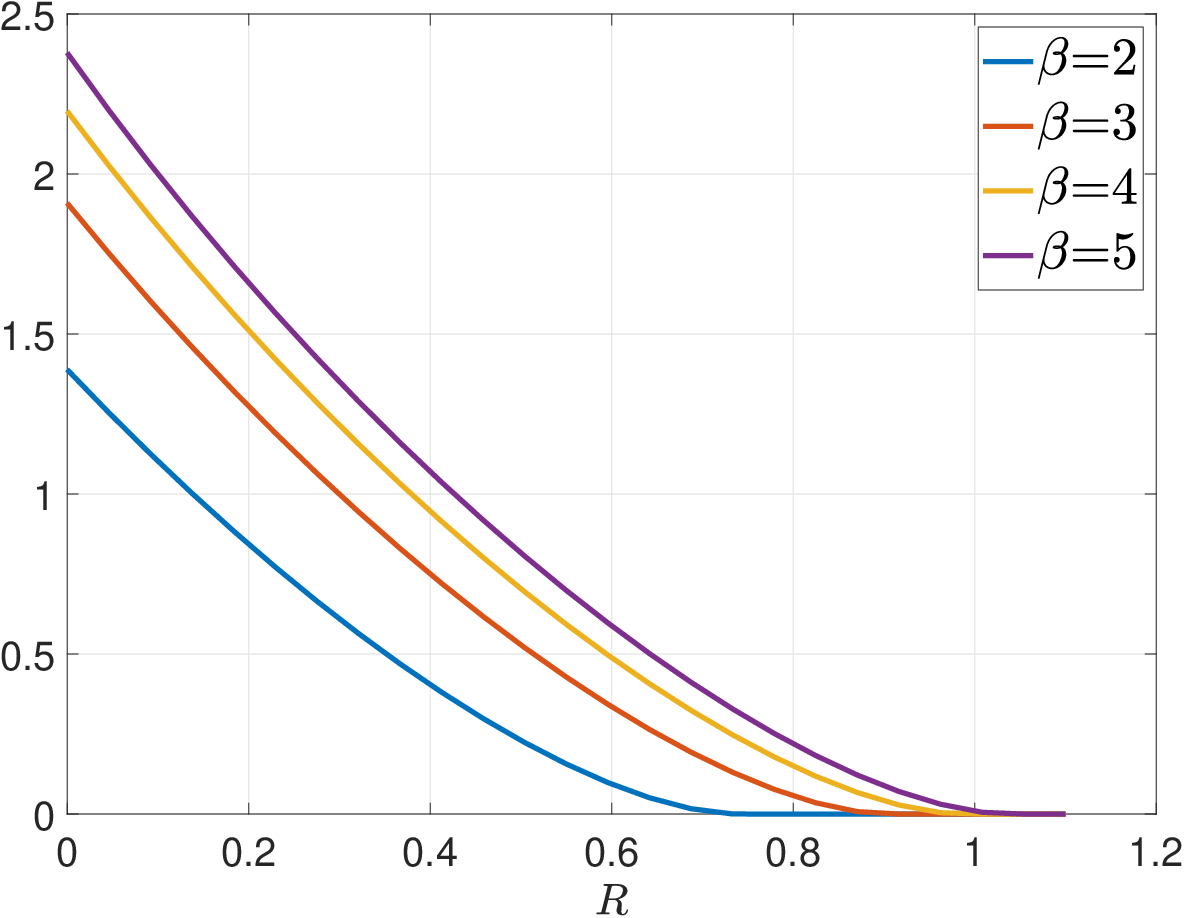
Figure 3: Upper and lower bounds on C⁡(𝖣𝖭𝖠⁡(5,β,W0))C(\mathsf{DNA}(5,\beta,W_{0})) as a function of β\beta (in nats).
Refer to caption
Figure 4: Lower bound on the reliability function E∗​(R,𝖣𝖭𝖠⁡(5,β,W0),{M})E^{*}(R,\mathsf{DNA}(5,\beta,W_{0}),\{M\}) as a function of RR (in nats).

VII Summary and Open Problems

In this paper we have derived lower and upper bounds on the capacity of the memoryless sequencing channel. In terms of lower bounds, we show that the lower bound which was only known for BSC (or symmetric) sequencing channels, and is restricted to a partial regime of the molecule length parameter β\beta and the channel noise, holds in fact for general DMCs and without any restrictions. We have shown that this bound is achievable by a universal decoder, and obtained asymptotic bounds on its error probability. This has revealed that the DNA channel suffers from outage: The random amplification vector QN+1Q^{N+1} is a measure of the quality of the channel, in terms of the conditional mutual information it induces. When the mutual information is larger than the required coding rate, the error probability decays fast – exponentially w.r.t. scaling KM=M​L=β​M​log⁡MK_{M}=ML=\beta M\log M. However, the probability that QN+1Q^{N+1} is such that the required coding rate is not supported, the error probability is large.1313 13 At least, we do not have a non-trivial bound for it. Our bound on the probability of such events is exponential w.r.t. scaling KM=MK_{M}=M and so this is the dominant error event. In terms of upper bounds (converse), we have refined the analysis of [42, 27] by introducing of a general distance function between molecules. This resulted a tighter upper bound, which agrees with the lower bound for a larger regime of β\beta and WW.

The following problems remain open for the memoryless sequencing channel:

  1. 1.

    Matching lower and upper bounds: It is tempting to conjecture that the lower bound of Theorem 5 is the true capacity for any β\beta and WW. This implies that the upper bound of Theorem 10 is the one to be tightened. However, as we have discussed after Theorem 10, it is conceivable that we have pushed the capability of the converse arguments of [42, 27] to their maximum, at least assuming reasonably complicated arguments.1414 14 Except perhaps, for the possibility of considering groups of molecules larger than pairs – as discussed after Theorem 10. Hence, it is of interest to find proof arguments of substantially different nature that would be capable of establishing capacity in the high-noise/low β\beta regime.

  2. 2.

    Upper bounds on the reliability function: The lower bound derived here (Theorem 8) is based on an analysis of the molecule duplicate vector SM∈[N]MS^{M}\in[N]^{M}. In the proof of the lower bond, the multinomial distribution of SMS^{M} – for which the components SmS_{m} are identically distributed but statistically dependent – is replaced by S~M∈[N]M\tilde{S}^{M}\in[N]^{M} which follows an i.i.d. Poisson distribution Pois​(α)\text{Pois}(\alpha). This facilitates the analysis, but may not be tight. Specifically, the analysis Lemma 20 is not tight in general. As an illustrative example, in the Poisson model, the probability that none of the molecules is sampled is given by

    ℙ[∩m∈[M]S~m=0]=(1−e−α)M=e−M​log⁡(1−e−α).\mathbb{P}\left[\cap_{m\in[M]}\tilde{S}_{m}=0\right]=(1-e^{-\alpha})^{M}=e^{-M\log(1-e^{-\alpha})}. (41)

    This probability is exponential w.r.t. MM and thus affect the exponential decay of the error probability at this scale. For example, E∗​(R)≤log⁡(1−e−α)E^{*}(R)\leq\log(1-e^{-\alpha}) because the error probability is large if none of the molecules have been sampled. By contrast, in the true multinomial model ℙ[∩m∈[M]Sm=0]=0\mathbb{P}[\cap_{m\in[M]}S_{m}=0]=0. It is therefore of interest to find tight tails bounds on the multinomial SMS^{M}, and utilize them to obtain upper bounds on the reliability function.

  3. 3.

    Tight finite blocklength bounds: Finite length bounds are of specific interest in this problem, since the second-order terms in this problem vanish very slow. In our arguments, the decay rate is either O⁡(1log⁡M)O(\frac{1}{\log M}) and occasionally or even O⁡(log⁡log⁡Mlog⁡M)O(\frac{\log\log M}{\log M}). This seems to be an inherent aspect of the problem. For example, consider a basic model in which N=MN=M, each molecule is sampled exactly once (with probability 11), and the sequencing channel is noiseless. Then, the capacity is the normalized logarithm of the possible number of sequences. The stars and bars model (see footnote 15) implies that it capacity is 1M​L​log⁡(M+Mβ−1M)\frac{1}{ML}\log{M+M^{\beta}-1\choose M}, which by standard approximation of the binomial coefficient is 1−1β+O⁡(1log⁡M)1-\frac{1}{\beta}+O(\frac{1}{\log M}).

Acknowledgment

The advice of Ido Tal regarding the computation of the bounds is acknowledged with gratitude.

Appendix A Proofs of Lower Bounds

In this section, we prove the lower (achievability) bounds. A roadmap for the various results proved is provided in Fig. 5.

Refer to caption
Figure 5: Roadmap for the proofs of the lower bounds (achievability). The used abbreviations are Lemma (L.), Proposition (P.), Theorem (T.) and Fact (F.). The result at the tail of an arrow is utilized to prove the result pointed by its head.

Based on Theorem 8, the proof of Theorem 5 is short and standard. Thus, we provide it here before the proof of Theorem 8, assuming the latter holds.

Proof:

Let an arbitrary input distribution, PX∈𝒫⁡(𝒳)P_{X}\in{\cal P}({\cal X}), be given. By the strict positivity of the binary KL divergence db(p∣∣q)>0d_{b}(p\mid\mid q)>0 for all p≠qp\neq q

∑d∈ℕ(1−∑i∈[d]θi)⋅db(θd1−∑i∈[d]θi||πα|≥d(d))≥0,\sum_{d\in\mathbb{N}}\left(1-\sum_{i\in[d]}\theta_{i}\right)\cdot d_{b}\left(\frac{\theta_{d}}{1-\sum_{i\in[d]}\theta_{i}}\,\middle|\middle|\,\pi_{\alpha|\geq d}(d)\right)\geq 0, (A.1)

and a simple calculation shows that equality holds if and only if θd=πα​(d)\theta_{d}=\pi_{\alpha}(d) for all d∈ℕ+d\in\mathbb{N}^{+}. Let RR be given so that

R<∑d∈ℕπα​(d)⋅I⁡(PX,W⊕d)−1β​(1−πα​(0)).R<\sum_{d\in\mathbb{N}}\pi_{\alpha}(d)\cdot I(P_{X},W^{\oplus d})-\frac{1}{\beta}(1-\pi_{\alpha}(0)). (A.2)

Since {πα​(d)}\{\pi_{\alpha}(d)\} does not belong to the feasible set (16) of the minimization (15), it holds that E∗​(R,𝖣𝖭𝖠,{M})>0E^{*}(R,\mathsf{DNA},\{M\})>0. Hence, there exists a sequence of codes-decoders (𝒞M,𝒟M)({\cal C}_{M},{\cal D}_{M}) so that the average error probability satisfies

1|𝒞M|​∑j∈[|𝒞M|]𝗉𝖾⁡(𝒞,𝒟∣xL​M​(j))≤e−Θ⁡(M).\frac{1}{|{\cal C}_{M}|}\sum_{j\in[|{\cal C}_{M}|]}\mathsf{pe}({\cal C},{\cal D}\mid x^{LM}(j))\leq e^{-\Theta(M)}. (A.3)

A similar bound can be proved for the maximal error probability for a codebook of rate slightly smaller, say R−δR-\delta, for some δ>0\delta>0 (and all MM sufficiently large) by expurgating half of the codewords from each codebook with the largest 𝗉𝖾⁡(𝒞,𝒟∣xL​M​(j))\mathsf{pe}({\cal C},{\cal D}\mid x^{LM}(j)). Thus, R−δR-\delta is an achievable rate for any ϵ∈(0,1)\epsilon\in(0,1) and so the lower bound on capacity follows. ∎ The rest of this section is devoted to the proof of Theorem 8.

A-A Preliminaries: Sampling Type Classes

Recall that at the sampling stage, the pool of LL molecules {xmL}m∈[M]\{x_{m}^{L}\}_{m\in[M]} is sampled NN times, where uN∈[M]Nu^{N}\in[M]^{N}, the molecule index vector, is such that un=mu_{n}=m if xmLx_{m}^{L} is the sampled molecule at the nnth sampling trial. Recall also the definitions of the molecule duplicate vector sM∈[N]Ms^{M}\in[N]^{M} and the amplification vector qN+1∈[M+1]N+1q^{N+1}\in[M+1]^{N+1} from Sec. II-B. The triplet (uN,sM,qN+1)(u^{N},s^{M},q^{N+1}) can be described by the empirical count operator (2) as sM=𝒩⁡(uN)s^{M}=\mathscr{\mathscr{N}}(u^{N}) and qN+1=𝒩⁡(sM)=𝒩(2)​(uN)q^{N+1}=\mathscr{\mathscr{N}}(s^{M})=\mathscr{\mathscr{N}}^{(2)}(u^{N}), and then, sampling type classes can be defined as follows: The molecule index type class of sMs^{M} is defined as

𝒯sM:={uN∈[M]N:𝒩⁡(uN)=sM},\mathscr{T}_{s^{M}}:=\left\{u^{N}\in[M]^{N}\colon\mathscr{\mathscr{N}}(u^{N})=s^{M}\right\}, (A.4)

and the molecule duplicate type class of a qN+1q^{N+1} is defined as

𝒯qN+1:={sM∈[N]M:𝒩⁡(sM)=qN+1}.\mathscr{T}_{q^{N+1}}:=\left\{s^{M}\in[N]^{M}\colon\mathscr{\mathscr{N}}(s^{M})=q^{N+1}\right\}. (A.5)

In a similar fashion, we define the amplification type class as

𝒯qN+1(2):={uN∈[M]N:𝒩(2)​(uN)=qN+1}.\mathscr{T}_{q^{N+1}}^{(2)}:=\left\{u^{N}\in[M]^{N}\colon\mathscr{\mathscr{N}}^{(2)}(u^{N})=q^{N+1}\right\}. (A.6)

Let

𝒬(M,N):={qN+1∈[M+1]N+1:∑d∈[N+1]qd=M,∑d∈[N+1]dqd=N}\mathscr{Q}(M,N):=\left\{q^{N+1}\in[M+1]^{N+1}\colon\sum_{d\in[N+1]}q_{d}=M,\;\sum_{d\in[N+1]}dq_{d}=N\right\} (A.7)

be the set of all valid amplification vectors for MM input molecules and NN output molecules. The next proposition provides a tight asymptotic scaling of the sizes of the molecule index type class, the molecule duplicate type class, and the amplification type class. This will be used in the proofs of the lower bounds on capacity and reliability function.

Proposition 15.

For a coverage depth α=NM>0\alpha=\frac{N}{M}>0:

  1. 1.

    The number of types is bounded as |𝒬⁡(M,N)|≤e[1+o⁡(1)]​2​π23​M|\mathscr{Q}(M,N)|\leq e^{[1+o(1)]\sqrt{\frac{2\pi^{2}}{3}M}}.

  2. 2.

    The size of the amplification type class is

    |𝒯qN+1(2)|=exp⁡[(1−q0M)⋅M​log⁡M+ϵM⋅M],|\mathscr{T}_{q^{N+1}}^{(2)}|=\exp\left[\left(1-\frac{q_{0}}{M}\right)\cdot M\log M+\epsilon_{M}\cdot M\right], (A.8)

    where |ϵM|≤log⁡α2​e|\epsilon_{M}|\leq\log\alpha^{2}e.

Proof:

∎

  1. 1.

    It is evident that each qN+1q^{N+1} uniquely defines a restricted partition of NN to at most M=NαM=\frac{N}{\alpha} summands (a bijection can be defined between qN+1∈𝒬⁡(M,N)q^{N+1}\in\mathscr{Q}(M,N) and a restricted partition). For example, qN+1=(M−5,2,2,,…0,1⏟qN−6,…,0,0)q^{N+1}=(M-5,2,2,,\ldots 0,\underbrace{1}_{q_{N-6}},\ldots,0,0) corresponds to the partition N=1+1+2+2+(N−6)N=1+1+2+2+(N-6). The number of restricted partitions is asymptotically bounded as claimed by the celebrated analysis of Hardy and Ramanujan, Uspensky, and Rademacher [2, Ch. 5].

  2. 2.

    Let sMs^{M} and qN+1q^{N+1} be such that 𝒩⁡(sM)=qN+1\mathscr{\mathscr{N}}(s^{M})=q^{N+1}. The exact value of |𝒯qN+1||\mathscr{T}_{q^{N+1}}| and |𝒯sM||\mathscr{T}_{s^{M}}| can be easily derived, and then |𝒯qN+1(2)||\mathscr{T}_{q^{N+1}}^{(2)}| is evaluated by |𝒯qN+1(2)|=|𝒯qN+1|⋅|𝒯sM||\mathscr{T}_{q^{N+1}}^{(2)}|=|\mathscr{T}_{q^{N+1}}|\cdot|\mathscr{T}_{s^{M}}|. The size of 𝒯qN+1\mathscr{T}_{q^{N+1}} is the number of unique permutations of the vector

    (0,0,…​0⏟q0,1,1​…​1⏟q1,…,d,d,…,d⏟qd,…)∈[N+1]M(\underbrace{0,0,\ldots 0}_{q_{0}},\underbrace{1,1\ldots 1}_{q_{1}},\ldots,\underbrace{d,d,\ldots,d}_{q_{d}},\ldots)\in[N+1]^{M} (A.9)

    given by

    |𝒯qN+1|=(Mq0,q1,…,qN)=M!∏d=0Nqd!.|\mathscr{T}_{q^{N+1}}|={M\choose q_{0},q_{1},\ldots,q_{N}}=\frac{M!}{\prod_{d=0}^{N}q_{d}!}. (A.10)

    It similarly holds that that size of 𝒯sM\mathscr{T}_{s^{M}} is

    |𝒯sM|=(Ns0,s1,…,sM−1)=N!∏m=0M−1sm!=N!∏d=0N(d!)qd,|\mathscr{T}_{s^{M}}|={N\choose s_{0},s_{1},\ldots,s_{M-1}}=\frac{N!}{\prod_{m=0}^{M-1}s_{m}!}=\frac{N!}{\prod_{d=0}^{N}(d!)^{q_{d}}}, (A.11)

    where the last equality holds by the definition qN+1=𝒩⁡(sM)q^{N+1}=\mathscr{N}(s^{M}). To prove the claimed upper bound we first bound |𝒯sM||\mathscr{T}_{s^{M}}| by the number of ways to choose each of the NN entries of uNu^{N} from a set of possible M−q0M-q_{0} molecules (without taking into account any other constraints on its empirical distribution). Thus

    |𝒯sM|≤NM−q0.|\mathscr{T}_{s^{M}}|\leq N^{M-q_{0}}. (A.12)

    To bound the size of 𝒯qN+1\mathscr{T}_{q^{N+1}}, let θd:=qdM\theta_{d}:=\frac{q_{d}}{M} so that θ=(θ0,…,θN)\theta=(\theta_{0},\ldots,\theta_{N}) is a p.m.f., and since ∑d∈[N+1]d​qd=N\sum_{d\in[N+1]}dq_{d}=N then ∑d∈[N+1]d​θd=α\sum_{d\in[N+1]}d\theta_{d}=\alpha must hold. Let H(θ):=−∑d∈[N+1]θdlogθdH(\theta):=-\sum_{d\in[N+1]}\theta_{d}\log\theta_{d} be the entropy of θ\theta. Then,

    |𝒯qN+1|​≤(a)​exp⁡[M⋅H⁡(θ)]​≤(b)​exp​[M⋅log⁡α​e],|\mathscr{T}_{q^{N+1}}|\overset{{\scriptstyle(a)}}{\leq}\exp\left[M\cdot H(\theta)\right]\overset{{\scriptstyle(b)}}{\leq}\exp\left[M\cdot\log\alpha e\right], (A.13)

    where (a)(a) is by the standard exponential upper bound of the multinomial coefficient with the entropy being the exponent (just as bounding the type class size in ordinary method of types [11, Lemma 2.3]), and (b)(b) is by upper bounding H⁡(θ)H(\theta) by the maximum entropy under the mean constraint α\alpha [11, Lemma 3.12 and Corollary 3.12] (it is easy to verify and well-known that the maximum entropy p.m.f. in this case is geometric). Hence, |𝒯qN+1|≤eΘ⁡(M)|\mathscr{T}_{q^{N+1}}|\leq e^{\Theta(M)}. Combining (A.13) with (A.12) and N=α​MN=\alpha M results in

    |𝒯qN+1(2)|=|𝒯qN+1|⋅|𝒯sM|≤e(M−q0)​log⁡N+Θ⁡(M)=e(M−q0)​log⁡M+Θ⁡(M).|\mathscr{T}_{q^{N+1}}^{(2)}|=|\mathscr{T}_{q^{N+1}}|\cdot|\mathscr{T}_{s^{M}}|\leq e^{(M-q_{0})\log N+\Theta(M)}=e^{(M-q_{0})\log M+\Theta(M)}. (A.14)

    To prove the claimed lower bound, let σm:=smN\sigma_{m}:=\frac{s_{m}}{N}, so that σ=(σ0,…,σM−1)\sigma=(\sigma_{0},\ldots,\sigma_{M-1}) is a p.m.f.. Here we lower bound |𝒯sM||\mathscr{T}_{s^{M}}| by the exponent of the entropy H⁡(σ)H(\sigma), divided by a factor which will be shown to be eΘ⁡(M)e^{\Theta(M)}. The proof is almost identical to the one used to lower bound the size of the type class (a multinomial coefficient) in the standard method of types: Considering σ\sigma as the empirical type of u∈[M]Nu\in[M]^{N} – an NN dimensional vector from alphabet of size MM – the exact number of possible types is (N+M−1M−1){N+M-1\choose M-1} (this follows from the stars and bars model.1515 15 The stars and bars model: Let a,n,k∈ℕ+a,n,k\in\mathbb{N}^{+} such that n≥kn\geq k and n>a​kn>ak. The number of ways to distribute nn stars into kk different bins (i.e., the number of integer solutions (x0,…,xk−1)(x_{0},\ldots,x_{k-1}) to ∑i∈[k]xi=n\sum_{i\in[k]}x_{i}=n) such that xi≥ax_{i}\geq a for all i∈[k]i\in[k] is (n−k⁡(a−1)−1k−1){n-k(a-1)-1\choose k-1}. See, also, e.g., [11, Ex. 2.1]). Then, the standard estimate on a type class size [8, Thm. 11.1.3] [11, Lemma 2.3] implies that1616 16 In the stated results in both [8, Thm. 11.1.3] and [11, Lemma 2.3], as well as in their proofs, the pre-exponent is given by the inverse of (N+1)M(N+1)^{M}, the latter being an upper bound to the exact value (N+M−1M−1){N+M-1\choose M-1}. Such a bound is useful in the standard method of types, since in that analysis N→∞N\to\infty while the alphabet size is M=Θ⁡(1)M=\Theta(1). Here M→∞M\to\infty and N=α​M=Θ⁡(M)→∞N=\alpha M=\Theta(M)\to\infty and so a different bound is required. Nonetheless, the proof itself carries over verbatim, except for replacing the bound (N+1)M(N+1)^{M} with the exact value (N+M−1M−1){N+M-1\choose M-1}.

    |𝒯sM|≥1(N+M−1M−1)​exp⁡[N⋅H⁡(σ)].|\mathscr{T}_{s^{M}}|\geq\frac{1}{{N+M-1\choose M-1}}\exp\left[N\cdot H(\sigma)\right]. (A.15)

    By the standard entropy bound on the binomial coefficient

    (N+M−1M−1)≤e(N+M−1)⋅hb​(MN+M)≤e(α+1)​M⋅hb​(1α+1)=eΘ⁡(M),{N+M-1\choose M-1}\leq e^{(N+M-1)\cdot h_{b}(\frac{M}{N+M})}\leq e^{(\alpha+1)M\cdot h_{b}(\frac{1}{\alpha+1})}=e^{\Theta(M)}, (A.16)

    and so continuing (A.15)

    |𝒯sM|≥exp⁡[N⋅H⁡(σ)−Θ⁡(M)]≥exp⁡[N⋅min⁡H⁡(ζ)−Θ⁡(M)],|\mathscr{T}_{s^{M}}|\geq\exp\left[N\cdot H(\sigma)-\Theta(M)\right]\geq\exp\left[N\cdot\min H(\zeta)-\Theta(M)\right], (A.17)

    where the minimum is over p.m.f’s ζ\zeta which have support of M−q0M-q_{0}. We next show that the minimal entropy is obtained at

    ζ∗=1N​(0,0​…​0⏟q0,N−(M−q0−1),1,1​…,1,1,1,1,…​1⏟M−q0−1).\zeta^{*}=\frac{1}{N}(\underbrace{0,0\ldots 0}_{q_{0}},N-(M-q_{0}-1),\underbrace{1,1\ldots,1,1,1,1,\ldots 1}_{M-q_{0}-1}). (A.18)

    To see this, note that any other ζ~\tilde{\zeta} which is supported on exactly M−q0M-q_{0} indices, and has entries which are integer multiples of 1/N1/N is majorized by ζ∗\zeta^{*} [30].1717 17 For any aK∈ℝKa^{K}\in\mathbb{R}^{K}, let a↓K∈ℝKa_{\downarrow}^{K}\in\mathbb{R}^{K} be such that 𝒩⁡(aK)=𝒩⁡(a↓K)\mathscr{N}(a^{K})=\mathscr{N}(a_{\downarrow}^{K}) and the components of a↓Ka_{\downarrow}^{K} are sorted in descending order. Then aK∈ℝKa^{K}\in\mathbb{R}^{K} majorizes bK∈ℝKb^{K}\in\mathbb{R}^{K} if ∑i∈[k]a↓,i≥∑i∈[k]b↓,i\sum_{i\in[k]}a_{\downarrow,i}\geq\sum_{i\in[k]}b_{\downarrow,i} for all k∈[K]k\in[K]. It then follows from the Schur-concavity of the entropy function that H⁡(ζ∗)≤H⁡(ζ~)H(\zeta^{*})\leq H(\tilde{\zeta}) [30, Ch. 3.D.1]. The resulting entropy is then

    H⁡(ζ∗)\displaystyle H(\zeta^{*}) =[N−(M−q0−1)N]​log⁡[NN−(M−q0−1)]+(M−q0−1)N​log⁡N\displaystyle=\left[\frac{N-(M-q_{0}-1)}{N}\right]\log\left[\frac{N}{N-(M-q_{0}-1)}\right]+\frac{(M-q_{0}-1)}{N}\log N (A.19)
    ≥(M−q0−1)N​log⁡N.\displaystyle\geq\frac{(M-q_{0}-1)}{N}\log N. (A.20)

    Thus,

    |𝒯sM|\displaystyle|\mathscr{T}_{s^{M}}| ≥exp⁡[N⋅(M−q0−1)N​log⁡N−Θ⁡(M)]\displaystyle\geq\exp\left[N\cdot\frac{(M-q_{0}-1)}{N}\log N-\Theta(M)\right] (A.21)
    ≥exp⁡[(M−q0)​log⁡M−Θ⁡(M)].\displaystyle\geq\exp\left[(M-q_{0})\log M-\Theta(M)\right]. (A.22)

    The proof is completed since |𝒯qN+1(2)|=|𝒯qN+1|⋅|𝒯sM|≥|𝒯sM||\mathscr{T}_{q^{N+1}}^{(2)}|=|\mathscr{T}_{q^{N+1}}|\cdot|\mathscr{T}_{s^{M}}|\geq|\mathscr{T}_{s^{M}}| as |𝒯qN+1|≥1|\mathscr{T}_{q^{N+1}}|\geq 1.

A-B Preliminaries: The DNA Channel as a Mixture of Binomial Channels

In this section, we develop an alternative representation for the likelihood function of the DNA channel with a memoryless sequencing channel. In the DNA channel, each symbol in the codeword is independently sequenced a variable number of times, according to the number of times the molecule it belongs to was sampled in the sampling stage. As a result, the likelihood function of all symbols is a (random) mixture of binomial channels. In this section, we make this property explicit in the likelihood function.

Let xL​Mx^{LM} be the input and yL​Ny^{LN} be the corresponding output of the DNA channel. Assume, as usual, that the sampling step is such that Un∼Uniform​[M]U_{n}\sim\text{Uniform}[M], i.i.d., independent of xL​Mx^{LM}. The basic expression for the likelihood function starts from (6) and is further developed as follows:

ℒ⁡[yL​N∣xL​M]\displaystyle{\cal L}\left[y^{LN}\mid x^{LM}\right] =∑uN∈[M]Nℙ[UN=uN]∏n∈[N]WL[ynL∣xunL]\displaystyle=\sum_{u^{N}\in[M]^{N}}\mathbb{P}[U^{N}=u^{N}]\prod_{n\in[N]}W^{L}\left[y_{n}^{L}\mid x_{u_{n}}^{L}\right] (A.23)
=∑qN+1∈𝒬⁡(M,N)∑s∈𝒯qN+1∑u∈𝒯sMℙ[UN=uN]∏n=0NWL[ynL∣xunL]\displaystyle=\sum_{q^{N+1}\in\mathscr{Q}(M,N)}\sum_{s\in\mathscr{T}_{q^{N+1}}}\sum_{u\in\mathscr{T}_{s^{M}}}\mathbb{P}\left[U^{N}=u^{N}\right]\prod_{n=0}^{N}W^{L}\left[y_{n}^{L}\mid x_{u_{n}}^{L}\right] (A.24)
=∑qN+1∈𝒬⁡(M,N)∑s∈𝒯qN+1ℙ⁡[𝒯sM]​∑u∈𝒯sM1|𝒯sM|​∏n=0NWL​[ynL∣xunL]\displaystyle=\sum_{q^{N+1}\in\mathscr{Q}(M,N)}\sum_{s\in\mathscr{T}_{q^{N+1}}}\mathbb{P}\left[\mathscr{T}_{s^{M}}\right]\sum_{u\in\mathscr{T}_{s^{M}}}\frac{1}{|\mathscr{T}_{s^{M}}|}\prod_{n=0}^{N}W^{L}\left[y_{n}^{L}\mid x_{u_{n}}^{L}\right] (A.25)
=∑qN+1∈𝒬⁡(M,N)ℙ⁡[𝒯qN+1(2)]​∑u∈𝒯qN+1(2)1|𝒯qN+1(2)|​∏n=0NWL​[ynL∣xunL],\displaystyle=\sum_{q^{N+1}\in\mathscr{Q}(M,N)}\mathbb{P}\left[\mathscr{T}_{q^{N+1}}^{(2)}\right]\sum_{u\in\mathscr{T}_{q^{N+1}}^{(2)}}\frac{1}{|\mathscr{T}_{q^{N+1}}^{(2)}|}\prod_{n=0}^{N}W^{L}\left[y_{n}^{L}\mid x_{u_{n}}^{L}\right], (A.26)

where ℙ[𝒯qN+1(2)]=|𝒯qN+1(2)|⋅ℙ[UN=uN]=|𝒯qN+1(2)|/MN\mathbb{P}[\mathscr{T}_{q^{N+1}}^{(2)}]=|\mathscr{T}_{q^{N+1}}^{(2)}|\cdot\mathbb{P}[U^{N}=u^{N}]=|\mathscr{T}_{q^{N+1}}^{(2)}|/M^{N}.

Consider a fixed (uN,sM,qN+1)(u^{N},s^{M},q^{N+1}), where uN∈𝒯sMu^{N}\in\mathscr{T}_{s^{M}}, sM∈𝒯qN+1s^{M}\in\mathscr{T}_{q^{N+1}} and qN+1∈𝒬⁡(M,N)q^{N+1}\in\mathscr{Q}(M,N). We next present the conditional likelihood term, ∏n=0N−1WL​[ynL∣xunL]\prod_{n=0}^{N-1}W^{L}[y_{n}^{L}\mid x_{u_{n}}^{L}], in an alternative form, which better expresses the mixture-of-binomial nature of this channel. Specifically, in this form, the symbols of the molecules that were sampled the same number of times are grouped together. Let K=M​LK=ML be the total number of symbols in the codeword xL​Mx^{LM} and let aK∈𝒜Ka^{K}\in{\cal A}^{K} be their concatenation in an arbitrary fixed order. For concreteness, we choose the natural ordering, that is, the one which satisfies x0L=(a0,a1,…,aL−1)x_{0}^{L}=(a_{0},a_{1},\ldots,a_{L-1}), x1L=(aL,aL+1,…,a2​L−1)x_{1}^{L}=(a_{L},a_{L+1},\ldots,a_{2L-1}), etc. Given (uN,sM,qN+1)(u^{N},s^{M},q^{N+1}), when aka_{k} belongs to a molecule xmx_{m} which has been sampled dkd_{k} times, it has dkd_{k} output symbols in yL​Ny^{LN}. Let bkdk=(bk,0,…,bk,dk−1)∈𝒴dkb_{k}^{d_{k}}=(b_{k,0},\ldots,b_{k,d_{k}-1})\in{\cal Y}^{d_{k}} be those dkd_{k} output symbols, ordered according to their order in yy, and let (b∗)K=(b0d0,…,bK−1dK−1)(b^{*})^{K}=(b_{0}^{d_{0}},\ldots,b_{K-1}^{d_{K-1}}). It should be noted that dkd_{k}, the dimension of bkb_{k} may be different for each kk, and depends on (uN,sM,qN+1)(u^{N},s^{M},q^{N+1}). Furthermore, dk∈[N+1]d_{k}\in[N+1] since the maximal number of times a single molecule can be sampled is NN.1818 18 Which only occurs in the unlikely event that only a single molecule has been sampled NN times.

With this interpretation, we now express the likelihood function in terms of W⊕dW^{\oplus d}, the dd-order binomial extension of WW (Definition 4), Specifically, we summarize the correspondence between (xL​M,yL​N)(x^{LM},y^{LN}) and (aK,b∗K)(a^{K},b^{*K}) (with K=M​LK=ML) as follows: The molecule index vector uNu^{N} transforms an input-output pair (xL​M,yL​N)(x^{LM},y^{LN}) to an equivalent input-output pair (aK,b∗K)(a^{K},b^{*K}) and a partition {𝒦d​(uN)}d∈[N+1]\{{\cal K}_{d}(u^{N})\}_{d\in[N+1]} of [K]=[M​L][K]=[ML] with Kd=|𝒦d​(u)|=qd​LK_{d}=|{\cal K}_{d}(u)|=q_{d}L such that the dimension of bkdkb_{k}^{d_{k}}, is dk=dd_{k}=d if and only if k∈𝒦d​(uN)k\in{\cal K}_{d}(u^{N}). For brevity, we have omitted in this notation the explicit dependency of (aK,b∗K)(a^{K},b^{*K}) in (xL​M,yL​N)(x^{LM},y^{LN}). It thus holds that

ℒ[yL​N∣xL​M,uN]=∏d=0NW⊕d[b𝒦d​(uN)d∣a𝒦d​(uN)],{\cal L}\left[y^{LN}\mid x^{LM},u^{N}\right]=\prod_{d=0}^{N}W^{\oplus d}\left[b_{{\cal K}_{d}(u^{N})}^{d}\mid a_{{\cal K}_{d}(u^{N})}\right], (A.27)

and combining this with (A.26), leads to the likelihood form

ℒ[yL​N∣xL​M]=∑qN+1∈𝒬⁡(M,N)ℙ[UN∈𝒯qN+1(2)]∑uN∈𝒯qN+1(2)1|𝒯qN+1(2)|∏d=0NW⊕d[b𝒦d​(uN)d∣a𝒦d​(uN)].{\cal L}\left[y^{LN}\mid x^{LM}\right]=\sum_{q^{N+1}\in\mathscr{Q}(M,N)}\mathbb{P}\left[U^{N}\in\mathscr{T}_{q^{N+1}}^{(2)}\right]\sum_{u^{N}\in\mathscr{T}_{q^{N+1}}^{(2)}}\frac{1}{|\mathscr{T}_{q^{N+1}}^{(2)}|}\prod_{d=0}^{N}W^{\oplus d}\left[b_{{\cal K}_{d}(u^{N})}^{d}\mid a_{{\cal K}_{d}(u^{N})}\right]. (A.28)

For brevity, we further simplify 𝒦d≡𝒦d​(uN){\cal K}_{d}\equiv{\cal K}_{d}(u^{N}). Furthermore, we note that the likelihood (A.27), conditioned on uNu^{N}, is determined by the joint type in the dd-order binomial a𝒦d→b𝒦dda_{{\cal K}_{d}}\to b_{{\cal K}_{d}}^{d} channel given by

P^d​(xL​M,yL​N,uN):=𝒫⁡(a𝒦d,b𝒦dd)\hat{P}^{d}(x^{LM},y^{LN};u^{N}):=\mathscr{P}(a_{{\cal K}_{d}},b_{{\cal K}_{d}}^{d}) (A.29)

for all d∈[N+1]d\in[N+1].

A-C A Universal Decoder for the DNA Channel

When the codewords are chosen under the uniform probability distribution, the optimal decoding rule in terms of error probability is the (maximum likelihood) ML decoding rule. However, it is also well known that in random coding analysis of DMCs with a fixed composition ensemble, the ML rule can be replaced by the MMI rule, without degrading the random coding error exponent [10, Ch. 10] [10, Thm. IV.1]. Here, however, we will analyze the i.i.d. random coding ensemble, in which the M​L⋅|𝒞|ML\cdot|{\cal C}| symbols in the codebook 𝒞={xL​M​(j)}{\cal C}=\{x^{LM}(j)\} are drawn i.i.d. from a distribution PXP_{X}. In this ensemble, the codewords do not have fixed composition with probability 11 and so the standard MMI is not universal (see the discussion after the proof of Prop. 17 in the next subsection for the reason to preferring this ensemble of the fixed composition ensemble). Nonetheless, for this ensemble, the random coding exponent of the ML rule can be achieved by a variant of the MMI, which includes an additional penalty term.

In this section, we first briefly describe the standard MMI rule and then adapt it to DNA channel. We then modify the basic MMI with two penalty terms: One is related to the use of the i.i.d. ensemble (instead of the constant composition ensemble), and the other – to the sampling mechanism of the DNA channel.

Specifically, let 𝒜,ℬ{\cal A},{\cal B} be finite input and output alphabets (respectively), and let V:𝒜→ℬV\colon{\cal A}\to{\cal B} be a DMC. Then, the normalized log-likelihood of an output sequence bK∈ℬKb^{K}\in{\cal B}^{K}, conditioned on an input sequence aK∈𝒜Ka^{K}\in{\cal A}^{K}, is

1KlogVK(bK∣aK)=−H𝒫⁡(aK,bK)(B∣A)−D(𝒫(aK,bK)∣∣𝒫(aK)×V),\frac{1}{K}\log V^{K}(b^{K}\mid a^{K})=-H_{\mathscr{P}(a^{K},b^{K})}(B\mid A)-D\left(\mathscr{P}(a^{K},b^{K})\mid\mid\mathscr{P}(a^{K})\times V\right), (A.30)

where 𝒫⁡(aK,bK)\mathscr{P}(a^{K},b^{K}) is the empirical joint distribution of (aK,bK)∈𝒜K×ℬK(a^{K},b^{K})\in{\cal A}^{K}\times{\cal B}^{K}. For a codebook 𝒞⊆𝒜K{\cal C}\subseteq{\cal A}^{K}, and given an output vector bK∈ℬKb^{K}\in{\cal B}^{K}, the ML decoding rule is then

arg​maxaK∈𝒞1KlogVK(bK∣aK)=arg​minaK∈𝒞[H𝒫⁡(aK,bK)(B∣A)+D(𝒫(aK,bK)∣∣𝒫(aK)×V)].\argmax_{a^{K}\in{\cal C}}\frac{1}{K}\log V^{K}(b^{K}\mid a^{K})=\argmin_{a^{K}\in{\cal C}}\left[H_{\mathscr{P}(a^{K},b^{K})}(B\mid A)+D\left(\mathscr{P}(a^{K},b^{K})\mid\mid\mathscr{P}(a^{K})\times V\right)\right]. (A.31)

In universal decoding for DMCs, the decoding metric does not depend on the channel VV. A possible decoding rule replaces the normalized log-likelihood with its maximized version over all DMCs from 𝒜→ℬ{\cal A}\to{\cal B}. The resulting decoding rule is then

arg​maxaK∈𝒞⁡maxV​1K​log⁡VK​(bK∣aK)=arg​maxaK∈𝒞⁡H𝒫⁡(aK,bK)​(B∣A).\argmax_{a^{K}\in{\cal C}}\max_{V}\frac{1}{K}\log V^{K}(b^{K}\mid a^{K})=\argmax_{a^{K}\in{\cal C}}H_{\mathscr{P}(a^{K},b^{K})}(B\mid A). (A.32)

Equivalently, since H𝒫⁡(bK)​(B)H_{\mathscr{P}(b^{K})}(B) only depends on the output sequence, and thus is common to all codewords, the decoder chooses the codeword which maximizes the empirical mutual information I𝒫⁡(aK,bK)​(A,B).I_{\mathscr{P}(a^{K},b^{K})}(A;B). This decoder is called MMI, and evidently it does not depend on the channel VV.

When condition on uNu^{N}, the likelihood function of the DNA channel (A.27) corresponds to a mixture of binomial channels. The MMI can be generalized, in a straightforward manner, to the mixture of binomial channels as follows. Formally, consider a mixture of binomial channels, parameterized by (V,K,{𝒦d}d∈[K+1])(V,K,\{{\cal K}_{d}\}_{d\in[K+1]}) (where 𝒦d{\cal K}_{d} is a partition of [K][K]). Given a codebook 𝒞⊆𝒜K{\cal C}\subseteq{\cal A}^{K}, an MMI decoder for this channel can be defined as

arg​maxaK∈𝒞∑d∈ℕKdK⋅I𝒫⁡(a𝒦d,b𝒦dd)(A;Bd),\argmax_{a^{K}\in{\cal C}}\sum_{d\in\mathbb{N}}\frac{K_{d}}{K}\cdot I_{\mathscr{P}(a_{{\cal K}_{d}},b_{{\cal K}_{d}}^{d})}(A;B^{d}), (A.33)

which amounts to averaging of the empirical mutual information over the possible orders dd, while taking into account their proportion in the KK symbols.

Equipped with these preliminaries, we next develop a universal decoder for the DNA channel 𝖣𝖭𝖠={α,β,W}\mathsf{DNA}=\{\alpha,\beta,W\}. As said, the maximum-likelihood rule arg​maxj∈[|𝒞|]⁡ℒ​[yLN∣xLM​(j)]\argmax_{j\in[|{\cal C}|]}{\cal L}[y^{LN}\mid x^{LM}(j)] is the optimal decoder. Here, the main motivation for using the universal decoder is mostly in order to facilitate the analysis (with the additional benefit that the knowledge of the sequencing channel WW is not required). It is evident from (A.28) that the likelihood is a mixture (over uNu^{N}) of a mixture (over dd) of binomial channels. Had uNu^{N} been known to the decoder, a possible universal decoder is the MMI for the mixture of binomial channels stated in (A.33), which in the DNA channel amounts to the metric

log⁡ℒ⁡(yL​N∣xL​M;uN)=∑d∈[K+1]qd​L⋅IP^d​(xL​M,yL​N,uN)​(A,Bd),\log\mathcal{L}(y^{LN}\mid x^{LM};u^{N})=\sum_{d\in[K+1]}q_{d}L\cdot I_{\hat{P}^{d}(x^{LM},y^{LN};u^{N})}(A;B^{d}), (A.34)

where qN+1=𝒩(2)​(uN)q^{N+1}=\mathscr{N}^{(2)}(u^{N}). For the DNA channel, uNu^{N} is unknown, and so we propose to further maximize this metric over uN∈𝒯qN+1(2)u^{N}\in\mathscr{T}_{q^{N+1}}^{(2)}, albeit with a penalty term related to |𝒯qN+1(2)||\mathscr{T}_{q^{N+1}}^{(2)}|. From a technical perspective, this penalty will compensate for a standard union bound that will be used in the random coding analysis, as is common in related scenarios (e.g., universal decoding for joint source-channel coding [9]). Intuitively, this penalty will favor less the likelihood of {uN}\{u^{N}\} which belong to a large amplification type class 𝒯qN+1(2)\mathscr{T}_{q^{N+1}}^{(2)}. More precisely, the proposed penalty is the first order term in the asymptotic expansion of the logarithm of the size of |𝒯qN+1(2)||\mathscr{T}_{q^{N+1}}^{(2)}|, rather than its exact size, which according to Prop. 15, is

log⁡|𝒯qN+1(2)|=(M−q0)​log⁡M+O⁡(M).\log|\mathscr{T}_{q^{N+1}}^{(2)}|=(M-q_{0})\log M+O(M). (A.35)

Moreover, the maximization will not be over all possible {uN}\{u^{N}\}. Instead, a finite d¯\overline{d} is set, and only uNu^{N} for which qN+1=𝒩(2)​(uN)∈𝒬d¯​(M,N)q^{N+1}=\mathscr{N}^{(2)}(u^{N})\in\mathscr{Q}_{\overline{d}}(M,N) are feasible in the maximization, where

𝒬d¯​(M,N):={qN+1∈𝒬⁡(M,N):qd=0​∀d≥d¯}.\mathscr{Q}_{\overline{d}}(M,N):=\left\{q^{N+1}\in\mathscr{Q}(M,N)\colon q_{d}=0\;\forall d\geq\overline{d}\right\}. (A.36)

That is, the set of candidate {qN+1}\{q^{N+1}\} does not include a single molecule being sampled more than d¯\overline{d} times. This restriction will be instrumental for the analysis.

In addition to the penalty term log⁡|𝒯qN+1(2)|\log|\mathscr{T}_{q^{N+1}}^{(2)}|, we add another penalty term related to the choice of i.i.d. ensemble, instead of the fixed composition ensemble. To this end, let P^d​(xL​M,uN)\hat{P}^{d}(x^{LM};u^{N}) be the xx-marginal of P^d​(xL​M,yL​N,uN)\hat{P}^{d}(x^{LM},y^{LN};u^{N}). Assuming an input distribution PXP_{X}, this penalty term for the dd order binomial channel, is the normalized asymptotic expansion of the probability that the input to the dd order binomial channel has type P^d​(xL​M,uN)\hat{P}^{d}(x^{LM};u^{N}), which is given by D(P^d(xL​M;uN)∣∣PX)D(\hat{P}^{d}(x^{LM};u^{N})\mid\mid P_{X}).

The result is that the universal decoder replaces log-likelihood log⁡ℒ⁡[yL​N∣xL​M​(j)]\log{\cal L}[y^{LN}\mid x^{LM}(j)] with the following universal metric:

log⁡ℒu​[yL​N∣xL​M​(j)]=maxqN+1∈𝒬d¯​(M,N)⁡maxs∈𝒯qN+1​maxu∈𝒯sM⁡λ⁡(yL​N∣xL​M​(j);qN+1,sM,uN),\log{\cal L}_{\text{u}}[y^{LN}\mid x^{LM}(j)]=\max_{q^{N+1}\in\mathscr{Q}_{\overline{d}}(M,N)}\max_{s\in\mathscr{T}_{q^{N+1}}}\max_{u\in\mathscr{T}_{s^{M}}}\lambda(y^{LN}\mid x^{LM}(j);q^{N+1},s^{M},u^{N}), (A.37)

with λ⁡(yL​N∣xL​M;uN)\lambda(y^{LN}\mid x^{LM};u^{N}) is defined as

λ(yL​N∣xL​M;uN):=−(M−q0)logM+∑d∈[N+1]qdL⋅[D(P^d(xL​M;uN)∣∣PX)+IP^d​(xL​M,yL​N,uN)(A;Bd)],\lambda(y^{LN}\mid x^{LM};u^{N}):=-(M-q_{0})\log M+\sum_{d\in[N+1]}q_{d}L\cdot\left[D(\hat{P}^{d}(x^{LM};u^{N})\mid\mid P_{X})+I_{\hat{P}^{d}(x^{LM},y^{LN};u^{N})}(A;B^{d})\right], (A.38)

where qN+1=𝒩(2)​(uN)q^{N+1}=\mathscr{N}^{(2)}(u^{N}) in (A.38) is assumed. As a final remark, we mention that constructing the decoder on the basis of empirical types on a “symbol-wise” level is only justified here since the sequencing channel WLW^{L} is a product of LL DMCs W:𝒳→𝒴W\colon{\cal X}\to{\cal Y}.

A-D Random-Coding Error Probability Analysis for a Given QN+1Q^{N+1}

We now turn to analyze the random coding error exponent of the proposed universal decoder for the following random ensemble: The M​L⋅|𝒞|ML\cdot|{\cal C}| symbols in the codebook 𝒞={xL​M​(j)}{\cal C}=\{x^{LM}(j)\} are drawn i.i.d. from a distribution PXP_{X}. We evaluate the average error probability conditioned on QN+1=qN+1Q^{N+1}=q^{N+1} and show that that if the rate does not cross a prescribed threshold, then the average error probability decays exponentially in KM=M​L=β​M​log⁡MK_{M}=ML=\beta M\log M. The proof for the bounds on the reliability function of Theorems 8 and 9 is concluded in the next subsections by averaging over QN+1Q^{N+1}. As mentioned in the previous subsection, we set d¯∈ℕ+\overline{d}\in\mathbb{N}^{+} and only consider qN+1∈𝒬d¯​(M,N)q^{N+1}\in\mathscr{Q}_{\overline{d}}(M,N), that is qN+1q^{N+1} for which qd=0q_{d}=0 for all d≥d¯d\geq\overline{d}.

As we have seen, the likelihood function of the DNA channel is obtained by a mixture of binomial channels. To facilitate the random coding analysis, we first state a general result regarding exponential probability bounds for such channels. Since our statements are for general DMCs, we denote the blocklength by K∈ℕ+K\in\mathbb{N}^{+}, the input alphabet by 𝒜{\cal A} and the output alphabet by ℬ{\cal B} in order to avoid confusion with the notation of the DNA channel.

Let V:𝒜→ℬV\colon{\cal A}\to{\cal B} be a DMC, and let V⊕d:𝒜→ℬdV^{\oplus d}\colon{\cal A}\to{\cal B}^{d} be its binomial extension. For a blocklength KK, consider a mixture of dd-order binomial channels (V,K,{𝒦d}d∈ℕ+)(V,K,\{{\cal K}_{d}\}_{d\in\mathbb{N}^{+}}) where {𝒦d}d∈ℕ+\{{\cal K}_{d}\}_{d\in\mathbb{N}^{+}} is a partition of [K][K]. Let aKa^{K} (respectively bKb^{K}) be the input (respectively output) to this channel, and assume that 𝒦d⊆[K]{\cal K}_{d}\subseteq[K] are the indices of inputs aka_{k} which are input to V⊕dV^{\oplus d}. We denote a𝒦d=(ak)k∈𝒦da_{{\cal K}_{d}}=(a_{k})_{k\in{\cal K}_{d}} according to increasing order in 𝒦d{\cal K}_{d}, and use a similar notation for bKb^{K}. Note that 𝒦d{\cal K}_{d} can be the empty set, but these sets will simply be ignored in a natural way in the next derivations. We thus assume that

ℙ[B(∗K)=(b∗)K∣AK=aK]=∏d=0∞V⊕d[b𝒦dd∣a𝒦d]=∏d=0∞∏k∈𝒦dV⊕d[bkd∣ak]=∏d=0∞∏k∈𝒦d∏i=0d−1V[bk,i∣ak].\mathbb{P}\left[B^{(*K)}=(b^{*})^{K}\mid A^{K}=a^{K}\right]=\prod_{d=0}^{\infty}V^{\oplus d}\left[b_{{\cal K}_{d}}^{d}\mid a_{{\cal K}_{d}}\right]=\prod_{d=0}^{\infty}\prod_{k\in{\cal K}_{d}}V^{\oplus d}\left[b_{k}^{d}\mid a_{k}\right]=\prod_{d=0}^{\infty}\prod_{k\in{\cal K}_{d}}\prod_{i=0}^{d-1}V\left[b_{k,i}\mid a_{k}\right]. (A.39)

Note that in the last expression, (b∗)K(b^{*})^{K} designates an output vector whose components may have different dimensions (according to the order dd). The following is a generalization of well-known bounds:

Proposition 16.

Let V:𝒜→ℬV\colon{\cal A}\to{\cal B} be a DMC and let V⊕dV^{\oplus d} be its dd-order binomial extension. Assume that AK∈𝒜KA^{K}\in{\cal A}^{K} has i.i.d. components distributed according to PAP_{A}. Let {𝒦d}d∈ℕ+\{{\cal K}_{d}\}_{d\in\mathbb{N}^{+}} be a partition of [K][K] and Kd=|𝒦d|K_{d}=|{\cal K}_{d}|. Assume further that Kd=0K_{d}=0 for all d≥d¯d\geq\overline{d}. Then:

  1. 1.

    If b𝒦db_{{\cal K}_{d}} is fixed and has type QBd(d)Q_{B^{d}}^{(d)} for d∈ℕ+d\in\mathbb{N}^{+}, then for any given sequence of joint type QA​Bd(d)Q_{AB^{d}}^{(d)} (whose BB-marginals all agree with QB(d)Q_{B}^{(d)})

    ℙ[⋂d∈[d¯](A𝒦d,b𝒦dd)∈𝒯Kd(QA​Bd(d))]≤exp{−K⋅[∑d∈[K]KdK⋅(D(QA∣∣PA)+IQ(d)(A;Bd)+O(|𝒜|​|ℬ|d​log⁡KdKd))]}.\mathbb{P}\left[\bigcap_{d\in[\overline{d}]}(A_{{\cal K}_{d}},b_{{\cal K}_{d}}^{d})\in{\cal T}_{K_{d}}(Q_{AB^{d}}^{(d)})\right]\leq\\ \exp\left\{-K\cdot\left[\sum_{d\in[K]}\frac{K_{d}}{K}\cdot\left(D(Q_{A}\mid\mid P_{A})+I_{Q^{(d)}}(A;B^{d})+O\left(\frac{|{\cal A}||{\cal B}|^{d}\log K_{d}}{K_{d}}\right)\right)\right]\right\}. (A.40)
  2. 2.

    If Bk∼V⊕d(⋅|Ak)B_{k}\sim V^{\oplus d}(\cdot|A_{k}) independently for all k∈𝒦dk\in{\cal K}_{d} and all d∈[K]d\in[K], that is ℙ⁡[B∗K=b∗K∣AK=aK]\mathbb{P}[B^{*K}=b^{*K}\mid A^{K}=a^{K}] is as in (A.39), then

    ℙ[⋂d∈[d¯](A𝒦d,B𝒦dd)∈𝒯Kd(d)(QA​Bd(d))]≤exp{−K⋅[∑d∈[K]KdK⋅(D(QA(d)∣∣PA)+D(QB|A(d)∣∣V⊕d|QA)+O(|𝒜|​|ℬ|d​log⁡KdKd))]}.\mathbb{P}\left[\bigcap_{d\in[\overline{d}]}(A_{{\cal K}_{d}},B_{{\cal K}_{d}}^{d})\in{\cal T}_{K_{d}}^{(d)}(Q_{AB^{d}}^{(d)})\right]\leq\\ \exp\left\{-K\cdot\left[\sum_{d\in[K]}\frac{K_{d}}{K}\cdot\left(D(Q_{A}^{(d)}\mid\mid P_{A})+D(Q_{B|A}^{(d)}\mid\mid V^{\oplus d}|Q_{A})+O\left(\frac{|{\cal A}||{\cal B}|^{d}\log K_{d}}{K_{d}}\right)\right)\right]\right\}. (A.41)
Proof:

First assume that Kd=KK_{d}=K for some dd. The proof then extends in a straightforward manner the same results obtained by the standard method of types [11, 10]. Specifically, by arguments as in [11, Problem 2.3] for (A.40), and [11, Lemma 2.6] for (A.41). The second-order term O⁡(|𝒜|​|ℬ|d⋅(log⁡K)/K)O(|{\cal A}||{\cal B}|^{d}\cdot(\log K)/K) follows from the standard estimate [11, Lemma 2.2] on the number of joint types for V⊕d:𝒜→ℬdV^{\oplus d}\colon{\cal A}\to{\cal B}^{d}

|𝒫K​(𝒜×ℬd)|≤(K+1)|𝒜|​|ℬ|d=exp⁡[|𝒜|​|ℬ|d⋅log⁡(K+1)].|{\cal P}_{K}({\cal A}\times{\cal B}^{d})|\leq(K+1)^{|{\cal A}||{\cal B}|^{d}}=\exp\left[|{\cal A}||{\cal B}|^{d}\cdot\log(K+1)\right]. (A.42)

The bound for a general partition {𝒦d}\{{\cal K}_{d}\} then follows from the statistical independence of the inputs to the various order-dd binomial channels. ∎We emphasize that since Kd=0K_{d}=0 for all d≥d¯d\geq\overline{d}, the second-order term in (A.40) and (A.41) is uniformly bounded as O⁡(|𝒜|​|ℬ|d¯⋅(log⁡K)/K)O(|{\cal A}||{\cal B}|^{\overline{d}}\cdot(\log K)/K). As common, (A.40) will be used to analyze the probability that a competing codeword has larger decoding metric than the true codeword (for a given output), and (A.41) will be used to analyze the probability of observing a codeword and its output under the random coding assumption and the channel’s randomness. We now have the following random coding bound conditioned on QN+1=qN+1Q^{N+1}=q^{N+1}:

Proposition 17.

Consider the DNA channel 𝖣𝖭𝖠=(α,β,W)\mathsf{DNA}=(\alpha,\beta,W). Let qN+1∈𝒬⁡(M,N)q^{N+1}\in\mathscr{Q}(M,N) be given. Suppose that the codebook 𝒞{\cal C} is drawn with i.i.d. symbols and codewords from PX∈𝒫⁡(𝒳)P_{X}\in{\cal P}({\cal X}). Let the universal decoder 𝒟u{\cal D}_{u} be such that yL​N∈𝒟u​(j)y^{LN}\in{\cal D}_{\text{u}}(j) if

j∈arg​maxj~∈[|𝒞|]​log​ℒu​(yLN∣xLM​(j~)).j\in\argmax_{\tilde{j}\in[|{\cal C}|]}\log\mathcal{L}_{\text{u}}(y^{LN}\mid x^{LM}(\tilde{j})). (A.43)

Then,

𝔼𝒞[𝗉𝖾(𝒞,𝒟u∣xL​M(0) stored,QN+1=qN+1)]≤exp[−ML⋅(Ed¯(R,𝖣𝖭𝖠∣qN+1)−Od¯(1M​log⁡M))],\mathbb{E}_{{\cal C}}\left[\mathsf{pe}({\cal C},{\cal D}_{\text{u}}\mid x^{LM}(0)\text{ \emph{stored}},Q^{N+1}=q^{N+1})\right]\leq\\ \exp\left[-ML\cdot\left(E_{\overline{d}}(R,\mathsf{DNA}\mid q^{N+1})-O_{\overline{d}}\left(\frac{1}{\sqrt{M}\log M}\right)\right)\right], (A.44)

where 𝔼𝒞​[⋅]\mathbb{E}_{{\cal C}}[\cdot] denotes expectation over the random codebook, 𝗉𝖾(𝒞,𝖣u∣xL​M(j),qN+1)\mathsf{pe}({\cal C},\mathsf{D_{\text{u}}}\mid x^{LM}(j),q^{N+1}) is a conditional version of the error probability (9) and

Ed¯(R,𝖣𝖭𝖠∣qN+1):=min{QA​Bd(d)}d∈[d¯+1]∑d∈[d¯+1]qdM⋅(D(QA(d)∣∣PX)+D(QBd|A(d)∣∣V⊕d∣QA))+[∑d∈[d¯+1]qdM⋅(D(QA(d)∣∣PX)+IQ(d)(A;Bd))−1β(1−q0M)−R]+.E_{\overline{d}}(R,\mathsf{DNA}\mid q^{N+1}):=\min_{\{Q_{AB^{d}}^{(d)}\}_{d\in[\overline{d}+1]}}\sum_{d\in[\overline{d}+1]}\frac{q_{d}}{M}\cdot\left(D(Q_{A}^{(d)}\mid\mid P_{X})+D(Q_{B^{d}|A}^{(d)}\mid\mid V^{\oplus d}\mid Q_{A})\right)\\ +\left[\sum_{d\in[\overline{d}+1]}\frac{q_{d}}{M}\cdot\left(D(Q_{A}^{(d)}\mid\mid P_{X})+I_{Q^{(d)}}(A;B^{d})\right)-\frac{1}{\beta}\left(1-\frac{q_{0}}{M}\right)-R\right]_{+}. (A.45)
Proof:

Since all sM∈𝒯qN+1s^{M}\in\mathscr{T}_{q^{N+1}} are equiprobable, and all uN∈𝒯qN+1(2)u^{N}\in\mathscr{T}_{q^{N+1}}^{(2)} are equiprobable too, symmetry implies that we can condition on an arbitrary sM∈𝒯qN+1s^{M}\in\mathscr{T}_{q^{N+1}} as well as an arbitrary uN∈𝒯sM=𝒯qN+1(2)u^{N}\in\mathscr{T}_{s^{M}}=\mathscr{T}_{q^{N+1}}^{(2)}. We bound the average conditional error probability in the following standard way, which comprises two steps. First, we condition on the randomly chosen stored codeword, xL​M​(1)x^{LM}(1), and the corresponding channel output, yL​Ny^{LN}, and compute the probability that a single random codeword has a larger decoding metric than ℒu​(yL​N∣xL​M​(0))\mathcal{L}_{\text{u}}(y^{LN}\mid x^{LM}(0)), and then we take a clipped union bound over eM​L​R−1e^{MLR}-1 competing codewords. Second, we compute the average over xL​M​(0),yL​Nx^{LM}(0),y^{LN}, connected via the DNA channel.

We begin with the first step. Assume that xL​M​(0)≡xL​Mx^{LM}(0)\equiv x^{LM} was stored and yL​Ny^{LN} was the output, and consider a competing random codeword xL​M​(j)≡X~L​Mx^{LM}(j)\equiv\tilde{X}^{LM} for some j∈[|𝒞|]\{0}j\in[|{\cal C}|]\backslash\{0\} (whose M​LML symbols are PXP_{X}-i.i.d.). Denote temporarily, for brevity, the event

ℰ:={XL​M​(1)=xL​M,YL​N=yL​N,QN+1=qN+1,SM=sM,UN=uN}.{\cal E}:=\left\{X^{LM}(1)=x^{LM},Y^{LN}=y^{LN},Q^{N+1}=q^{N+1},S^{M}=s^{M},U^{N}=u^{N}\right\}. (A.46)

The pairwise error probability is bounded as

ℙ⁡[log⁡ℒu​(yL​N∣X~L​M)≥log⁡ℒu​(yL​N∣xL​M)|ℰ]\displaystyle\mathbb{P}\left[\log\mathcal{L}_{\text{u}}(y^{LN}\mid\tilde{X}^{LM})\geq\log\mathcal{L}_{\text{u}}(y^{LN}\mid x^{LM})\,\middle|\,{\cal E}\right]
≤(a)​ℙ​[log⁡ℒu​(yL​N∣X~L​M)≥λ⁡(yL​N∣xL​M;uN)|ℰ]\displaystyle\overset{{\scriptstyle(a)}}{\leq}\mathbb{P}\left[\log\mathcal{L}_{\text{u}}(y^{LN}\mid\tilde{X}^{LM})\geq\lambda(y^{LN}\mid x^{LM};u^{N})\,\middle|\,{\cal E}\right] (A.47)
=ℙ⁡[maxq~N+1∈𝒬d¯​(M,N)⁡maxu~N∈𝒯qN+1~(2)⁡λ⁡(yL​N∣X~L​M;u~N)≥λ⁡(yL​N∣xL​M;uN)|ℰ]\displaystyle=\mathbb{P}\left[\max_{\tilde{q}^{N+1}\in\mathscr{Q}_{\overline{d}}(M,N)}\max_{\tilde{u}^{N}\in\mathscr{T}_{\tilde{q^{N+1}}}^{(2)}}\lambda(y^{LN}\mid\tilde{X}^{LM};\tilde{u}^{N})\geq\lambda(y^{LN}\mid x^{LM};u^{N})\,\middle|\,{\cal E}\right] (A.48)
≤(b)​∑q~N+1∈𝒬d¯​(M,N)∑u~N∈𝒯qN+1~(2)ℙ⁡[λ⁡(yL​N∣X~L​M;u~N)≥λ⁡(yL​N∣xL​M;uN)|ℰ]\displaystyle\overset{{\scriptstyle(b)}}{\leq}\sum_{\tilde{q}^{N+1}\in\mathscr{Q}_{\overline{d}}(M,N)}\sum_{\tilde{u}^{N}\in\mathscr{T}_{\tilde{q^{N+1}}}^{(2)}}\mathbb{P}\left[\lambda(y^{LN}\mid\tilde{X}^{LM};\tilde{u}^{N})\geq\lambda(y^{LN}\mid x^{LM};u^{N})\,\middle|\,{\cal E}\right] (A.49)
≤(c)​eO⁡(M)​NM−q~0​maxq~N+1∈𝒬d¯​(M,N)​maxu~∈𝒯qN+1~(2)⋅ℙ⁡[λ⁡(yL​N∣X~L​M;u~N)≥λ⁡(yL​N∣xL​M;uN)|ℰ],\displaystyle\overset{{\scriptstyle(c)}}{\leq}e^{O(\sqrt{M})}N^{M-\tilde{q}_{0}}\max_{\tilde{q}^{N+1}\in\mathscr{Q}_{\overline{d}}(M,N)}\max_{\tilde{u}\in\mathscr{T}_{\tilde{q^{N+1}}}^{(2)}}\cdot\mathbb{P}\left[\lambda(y^{LN}\mid\tilde{X}^{LM};\tilde{u}^{N})\geq\lambda(y^{LN}\mid x^{LM};u^{N})\,\middle|\,{\cal E}\right], (A.50)

where (a)(a) follows since from the definition of the universal metric log⁡ℒu​(yL​N∣xL​M)\log\mathcal{L}_{\text{u}}(y^{LN}\mid x^{LM}) in (A.37)

log⁡ℒu​(yL​N∣xL​M)≥λ⁡(yL​N∣xL​M;uN)\log\mathcal{L}_{\text{u}}(y^{LN}\mid x^{LM})\geq\lambda(y^{LN}\mid x^{LM};u^{N}) (A.51)

[using the possibly sub-optimal choice uNu^{N} in (A.37)], (b)(b) follows from the union bound, and (c)(c) follows from Prop. 15. We next evaluate the inner probability for a specific choice of u~N\tilde{u}^{N}. The value of λ⁡(yL​N∣x~L​M;u~N)\lambda(y^{LN}\mid\tilde{x}^{LM};\tilde{u}^{N}) is equivalently determined by (A~𝒦d,b𝒦dd)d∈[d¯+1](\tilde{A}_{{\cal K}_{d}},b_{{\cal K}_{d}}^{d})_{d\in[\overline{d}+1]} corresponding to (u~N,x~L​M,yL​N)(\tilde{u}^{N},\tilde{x}^{LM},y^{LN}), where the symbols A~K∈𝒜K\tilde{A}^{K}\in{\cal A}^{K} are drawn i.i.d. according to PXP_{X}. Letting {Q~A​Bd(d)}d∈[d¯+1]\{\tilde{Q}_{AB^{d}}^{(d)}\}_{d\in[\overline{d}+1]} be a collection of types with Q~Bd(d)=QBd(d)=𝒫⁡(b𝒦dd)\tilde{Q}_{B^{d}}^{(d)}=Q_{B^{d}}^{(d)}=\mathscr{P}(b_{{\cal K}_{d}}^{d}), Prop. 16 states that

ℙ[⋂d∈[d¯+1]:qd≠0(A~𝒦d,b𝒦dd)∈𝒯Kd(Q~A​Bd(d))]\displaystyle\mathbb{P}\left[\bigcap_{d\in[\overline{d}+1]\colon q_{d}\neq 0}(\tilde{A}_{{\cal K}_{d}},b_{{\cal K}_{d}}^{d})\in{\cal T}_{K_{d}}(\tilde{Q}_{AB^{d}}^{(d)})\right]
≤exp{−ML⋅[∑d∈[d¯+1]:qd≠0qdM⋅(D(Q~A(d)∣∣PX)+IQ~(d)(A;Bd)+O(|𝒳|​|𝒴|d​log⁡L​qdL​qd))]}\displaystyle\leq\exp\left\{-ML\cdot\left[\sum_{d\in[\overline{d}+1]\colon q_{d}\neq 0}\frac{q_{d}}{M}\cdot\left(D(\tilde{Q}_{A}^{(d)}\mid\mid P_{X})+I_{\tilde{Q}^{(d)}}(A;B^{d})+O\left(\frac{|{\cal X}||{\cal Y}|^{d}\log Lq_{d}}{Lq_{d}}\right)\right)\right]\right\} (A.52)
≤exp{−ML⋅[∑d∈[d¯+1]:qd≠0qdM⋅(D(Q~A(d)∣∣PX)+IQ~(d)(A;Bd))+Od¯(log⁡(M​L)M​L)]}\displaystyle\leq\exp\left\{-ML\cdot\left[\sum_{d\in[\overline{d}+1]\colon q_{d}\neq 0}\frac{q_{d}}{M}\cdot\left(D(\tilde{Q}_{A}^{(d)}\mid\mid P_{X})+I_{\tilde{Q}^{(d)}}(A;B^{d})\right)+O_{\overline{d}}\left(\frac{\log(ML)}{ML}\right)\right]\right\} (A.53)

where the last inequality follows from

∑d∈[d¯+1]qdM⋅|𝒳|​|𝒴|d​log⁡(L​qd)L​qd=1M​L​∑d∈[d¯+1]|𝒳|​|𝒴|d​log⁡(L​qd)≤d¯​|𝒳|​|𝒴|d¯​log⁡(M​L)M​L=Od¯​(log⁡(M​L)M​L).\sum_{d\in[\overline{d}+1]}\frac{q_{d}}{M}\cdot\frac{|{\cal X}||{\cal Y}|^{d}\log(Lq_{d})}{Lq_{d}}=\frac{1}{ML}\sum_{d\in[\overline{d}+1]}|{\cal X}||{\cal Y}|^{d}\log(Lq_{d})\leq\overline{d}|{\cal X}||{\cal Y}|^{\overline{d}}\frac{\log(ML)}{ML}=O_{\overline{d}}\left(\frac{\log(ML)}{ML}\right). (A.54)

Next, we note that λ⁡(yL​N∣x~L​M;u~N)\lambda(y^{LN}\mid\tilde{x}^{LM};\tilde{u}^{N}) is determined by the empirical types of 𝒫⁡(A~𝒦d,b𝒦dd)=P^d​(x~L​M,yL​N,u~N)\mathscr{P}(\tilde{A}_{{\cal K}_{d}},b_{{\cal K}_{d}}^{d})=\hat{P}^{d}(\tilde{x}^{LM},y^{LN};\tilde{u}^{N}), for d∈[d¯+1]d\in[\overline{d}+1]. The number of possible types of (A~𝒦d,b𝒦dd)(\tilde{A}_{{\cal K}_{d}},b_{{\cal K}_{d}}^{d}) is less than (Kd+1)|𝒳|​|𝒴|d=(qd​L+1)|𝒳|​|𝒴|d=exp⁡[|𝒳|​|𝒴|d⋅log⁡(qd​L+1)](K_{d}+1)^{|{\cal X}||{\cal Y}|^{d}}=(q_{d}L+1)^{|{\cal X}||{\cal Y}|^{d}}=\exp\left[|{\cal X}||{\cal Y}|^{d}\cdot\log(q_{d}L+1)\right] [as in (A.42)]. Consequently, the number of possible sets of types {Q~A​Bd(d)}d∈[d¯+1]\{\tilde{Q}_{AB^{d}}^{(d)}\}_{d\in[\overline{d}+1]} is upper bounded by

∏d=0d¯exp⁡[|𝒳|​|𝒴|d⋅log⁡(qd​L+1)]≤exp⁡[d¯​|𝒳|​|𝒴|d¯⋅log⁡(M​L+1)]\prod_{d=0}^{\overline{d}}\exp\left[|{\cal X}||{\cal Y}|^{d}\cdot\log(q_{d}L+1)\right]\leq\exp\left[\overline{d}|{\cal X}||{\cal Y}|^{\overline{d}}\cdot\log(ML+1)\right] (A.55)

which is polynomial in K=M​LK=ML (for fixed d¯\overline{d}). By the union bound over those set of types

ℙ⁡[λ⁡(yL​N∣X~L​M;u~N)≥λ⁡(yL​N∣xL​M;uN)∣ℰ]\displaystyle\mathbb{P}\left[\lambda(y^{LN}\mid\tilde{X}^{LM};\tilde{u}^{N})\geq\lambda(y^{LN}\mid x^{LM};u^{N})\mid{\cal E}\right]
≤∑{Q~A​Bd(d)}d∈[d¯+1]ℙ[⋂d=0d¯(A~𝒦d,b𝒦dd)∈𝒯Kd(d)(Q~A​Bd(d))],\displaystyle\leq\sum_{\{\tilde{Q}_{AB^{d}}^{(d)}\}_{d\in[\overline{d}+1]}}\mathbb{P}\left[\bigcap_{d=0}^{\overline{d}}(\tilde{A}_{{\cal K}_{d}},b_{{\cal K}_{d}}^{d})\in{\cal T}_{K_{d}}^{(d)}(\tilde{Q}_{AB^{d}}^{(d)})\right], (A.56)

where the sum is over {Q~A​Bd(d)}d∈[d¯+1]\{\tilde{Q}_{AB^{d}}^{(d)}\}_{d\in[\overline{d}+1]} such that Q~Bd(d)=QBd(d)\tilde{Q}_{B^{d}}^{(d)}=Q_{B^{d}}^{(d)} and

−(M−q~0)logN+∑d∈[d¯+1]q~dL⋅(D(Q~A(d)∣∣PX)+IQ~A​B(d)(A;Bd))\displaystyle-(M-\tilde{q}_{0})\log N+\sum_{d\in[\overline{d}+1]}\tilde{q}_{d}L\cdot\left(D(\tilde{Q}_{A}^{(d)}\mid\mid P_{X})+I_{\tilde{Q}_{AB}^{(d)}}(A;B^{d})\right)
≥λ⁡(yL​N∣xL​M;uN)\displaystyle\geq\lambda(y^{LN}\mid x^{LM};u^{N})
=−(M−q0)logN+∑d∈[d¯+1]qdL⋅(D(P^d(xL​M;uN)∣∣PX)+IP^d​(xL​M,yL​N,uN)(A;Bd))\displaystyle=-(M-q_{0})\log N+\sum_{d\in[\overline{d}+1]}q_{d}L\cdot\left(D(\hat{P}^{d}(x^{LM};u^{N})\mid\mid P_{X})+I_{\hat{P}^{d}(x^{LM},y^{LN};u^{N})}(A;B^{d})\right) (A.57)

holds. By (A.53), (A.55), and the last display, we obtain that

ℙ⁡[λ⁡(yL​N∣X~L​M;u~N)≥λ⁡(yL​N∣xL​M;uN)∣ℰ]\displaystyle\mathbb{P}\left[\lambda(y^{LN}\mid\tilde{X}^{LM};\tilde{u}^{N})\geq\lambda(y^{LN}\mid x^{LM};u^{N})\mid{\cal E}\right]
≤eO⁡(log⁡(M​L))⋅exp⁡[−(M−q~0)​log⁡N+(M−q0)​log⁡N]\displaystyle\leq e^{O(\log(ML))}\cdot\exp\left[-(M-\tilde{q}_{0})\log N+(M-q_{0})\log N\right]
=×exp{−ML⋅[∑d∈[d¯+1]qdM(D(P^d(xL​M;uN)∣∣PX)+IP^d​(xL​M,yL​N,uN)(A;Bd))+Od¯(log⁡(M​L)M​L)]}.\displaystyle\hphantom{=}\times\exp\left\{-ML\cdot\left[\sum_{d\in[\overline{d}+1]}\frac{q_{d}}{M}\left(D(\hat{P}^{d}(x^{LM};u^{N})\mid\mid P_{X})+I_{\hat{P}^{d}(x^{LM},y^{LN};u^{N})}(A;B^{d})\right)+O_{\overline{d}}\left(\frac{\log(ML)}{ML}\right)\right]\right\}. (A.58)

Inserting this bound into (A.50), we then obtain

log⁡ℙ⁡[ℒu​(yL​N∣X~L​M)≥ℒu​(yL​N∣xL​M)∣ℰ]\displaystyle\log\mathbb{P}\left[\mathcal{L}_{\text{u}}(y^{LN}\mid\tilde{X}^{LM})\geq\mathcal{L}_{\text{u}}(y^{LN}\mid x^{LM})\mid{\cal E}\right]
≤O⁡(M)+(M−q0)​log⁡N\displaystyle\leq O(\sqrt{M})+(M-q_{0})\log N
==−ML⋅[∑d∈[d¯+1]qdM⋅(D(P^d(xL​M;uN)∣∣PX)+IP^d​(xL​M,yL​N,uN)(A;Bd))+Od¯(log⁡(M​L)M​L)]\displaystyle\hphantom{==}-ML\cdot\left[\sum_{d\in[\overline{d}+1]}\frac{q_{d}}{M}\cdot\left(D(\hat{P}^{d}(x^{LM};u^{N})\mid\mid P_{X})+I_{\hat{P}^{d}(x^{LM},y^{LN};u^{N})}(A;B^{d})\right)+O_{\overline{d}}\left(\frac{\log(ML)}{ML}\right)\right] (A.59)
=−ML⋅[∑d∈[d¯+1]qdM⋅(D(P^d(xL​M;uN)∣∣PX)+IP^d​(xL​M,yL​N,uN)(A;Bd))−1β(1−q0M)+O(1M​L)],\displaystyle=-ML\cdot\left[\sum_{d\in[\overline{d}+1]}\frac{q_{d}}{M}\cdot\left(D(\hat{P}^{d}(x^{LM};u^{N})\mid\mid P_{X})+I_{\hat{P}^{d}(x^{LM},y^{LN};u^{N})}(A;B^{d})\right)-\frac{1}{\beta}\left(1-\frac{q_{0}}{M}\right)+O\left(\frac{1}{\sqrt{M}L}\right)\right], (A.60)

where in (a)(a) we have used that α=NM\alpha=\frac{N}{M} is constant1919 19 In fact, α=o⁡(log⁡M)\alpha=o(\log M) suffices. and β=Llog⁡M\beta=\frac{L}{\log M}. This completes the bound on the pairwise error probability for a single competing codeword. Letting now 𝗉𝖾¯​(𝒞,𝒟u∣ℰ)\overline{\mathsf{pe}}({\cal C},{\cal D}_{\text{u}}\mid{\cal E}) be the conditional average error probability over all eM​L​R−1e^{MLR}-1 competing codewords, the clipped union bound implies

−1M​L​log⁡𝔼𝒞​[𝗉𝖾¯​(𝒞,𝒟u∣ℰ)]≥[∑d∈[d¯+1]qdM⋅(D(P^d(xL​M;uN)∣∣PX)+IP^d​(xL​M,yL​N,uN)(A;Bd))−1β(1−q0M)−R]+−O(1M​L).-\frac{1}{ML}\log\mathbb{E}_{{\cal C}}\left[\overline{\mathsf{pe}}({\cal C},{\cal D}_{\text{u}}\mid{\cal E})\right]\geq\\ \left[\sum_{d\in[\overline{d}+1]}\frac{q_{d}}{M}\cdot\left(D(\hat{P}^{d}(x^{LM};u^{N})\mid\mid P_{X})+I_{\hat{P}^{d}(x^{LM},y^{LN};u^{N})}(A;B^{d})\right)-\frac{1}{\beta}\left(1-\frac{q_{0}}{M}\right)-R\right]_{+}-O\left(\frac{1}{\sqrt{M}L}\right). (A.61)

This completes the first step of the proof.

We now move on to the second step in which we average over (XL​M≡XL​M​(1),YL​N)(X^{LM}\equiv X^{LM}(1),Y^{LN}). In the first step, we have seen that the pairwise error probability conditioned on (XL​M,YL​N)=(xL​M,yL​N)(X^{LM},Y^{LN})=(x^{LM},y^{LN}) depends on ∑d∈[d¯+1]qdM⋅D(P^d(xL​M;uN)∣∣PX)+∑d∈[d¯+1]qdMIP^d​(xL​M,yL​N,uN)(A;Bd)\sum_{d\in[\overline{d}+1]}\frac{q_{d}}{M}\cdot D(\hat{P}^{d}(x^{LM};u^{N})\mid\mid P_{X})+\sum_{d\in[\overline{d}+1]}\frac{q_{d}}{M}I_{\hat{P}^{d}(x^{LM},y^{LN};u^{N})}(A;B^{d}), which in turn depend on the types {P^d​(xL​M,yL​N,uN)}d∈[d¯+1]\{\hat{P}^{d}(x^{LM},y^{LN};u^{N})\}_{d\in[\overline{d}+1]}. We next evaluate the probability distribution of this term, conditioned on the given qN+1q^{N+1}, and an arbitrary representative uN∈𝒯qN+1(2)u^{N}\in\mathscr{T}_{q^{N+1}}^{(2)}. As in the first step, we denote P^d​(xL​M,yL​N,uN)=QA​Bd(d)\hat{P}^{d}(x^{LM},y^{LN};u^{N})=Q_{AB^{d}}^{(d)}. Prop. 16 states that in case the random output B𝒦ddB_{{\cal K}_{d}}^{d} is the result of A𝒦dA_{{\cal K}_{d}} passing in the channel V⊕dV^{\oplus d}, it holds that

ℙ[⋂d∈[d¯+1]:qd≠0(A𝒦d,B𝒦d)∈𝒯Kd(QA​Bd(d))]\displaystyle\mathbb{P}\left[\bigcap_{d\in[\overline{d}+1]\colon q_{d}\neq 0}(A_{{\cal K}_{d}},B_{{\cal K}_{d}})\in{\cal T}_{K_{d}}(Q_{AB^{d}}^{(d)})\right]
≤exp{−ML⋅[∑d∈[d¯+1]:qd≠0qdM⋅(D(QA(d)∣∣PX)+D(QBd|A(d)∣∣V⊕d∣QA))+Od¯(log⁡(M​L)M​L)]},\displaystyle\leq\exp\left\{-ML\cdot\left[\sum_{d\in[\overline{d}+1]\colon q_{d}\neq 0}\frac{q_{d}}{M}\cdot\left(D(Q_{A}^{(d)}\mid\mid P_{X})+D(Q_{B^{d}|A}^{(d)}\mid\mid V^{\oplus d}\mid Q_{A})\right)+O_{\overline{d}}\left(\frac{\log(ML)}{ML}\right)\right]\right\}, (A.62)

where the second-order term is bounded as in (A.54). Thus, for sM∈𝒯qN+1s^{M}\in\mathscr{T}_{q^{N+1}} and uN∈𝒯sMu^{N}\in\mathscr{T}_{s^{M}}

𝔼𝒞[𝗉𝖾(𝒞,𝒟u∣xL​M(1) stored,QN+1=qN+1)]\displaystyle\mathbb{E}_{{\cal C}}\left[\mathsf{pe}({\cal C},{\cal D}_{\text{u}}\mid x^{LM}(1)\text{ stored},\;Q^{N+1}=q^{N+1})\right]
=𝔼𝒞[𝗉𝖾(𝒞,𝒟u∣QN+1=qN+1,SM=sM,UN=uN)]\displaystyle=\mathbb{E}_{{\cal C}}\left[\mathsf{pe}({\cal C},{\cal D}_{\text{u}}\mid Q^{N+1}=q^{N+1},S^{M}=s^{M},U^{N}=u^{N})\right] (A.63)
=∑{QA​Bd(d)}d∈[d¯]ℙ[⋂d=0d¯(A𝒦d,B𝒦dd)∈𝒯Kd(QA​Bd(d))]⋅𝗉𝖾¯(𝒞,𝒟u∣ℰ).\displaystyle=\sum_{\{Q_{AB^{d}}^{(d)}\}_{d\in[\overline{d}]}}\mathbb{P}\left[\bigcap_{d=0}^{\overline{d}}(A_{{\cal K}_{d}},B_{{\cal K}_{d}}^{d})\in{\cal T}_{K_{d}}(Q_{AB^{d}}^{(d)})\right]\cdot\overline{\mathsf{pe}}({\cal C},{\cal D}_{\text{u}}\mid{\cal E}). (A.64)

By (A.61), (A.62) and the bound (A.55) on the total number of sets of types {QA​B(d)}d∈[d¯+1]\{Q_{AB}^{(d)}\}_{d\in[\overline{d}+1]} (which from (A.55) is polynomial in M​LML ) we obtain that

−1M​Llog𝔼𝒞[𝗉𝖾(𝒞,𝒟∣XL​M(1) stored,QN+1=qN+1)]\displaystyle-\frac{1}{ML}\log\mathbb{E}_{{\cal C}}\left[\mathsf{pe}({\cal C},{\cal D}\mid X^{LM}(1)\text{ stored},\;Q^{N+1}=q^{N+1})\right]
≥min{QA​B(d)}∑d∈[d¯+1]qdM⋅(D(QA(d)∣∣PX)+D(QBd|A(d)∣∣V⊕d|QA(d)))\displaystyle\geq\min_{\{Q_{AB}^{(d)}\}}\sum_{d\in[\overline{d}+1]}\frac{q_{d}}{M}\cdot\left(D(Q_{A}^{(d)}\mid\mid P_{X})+D(Q_{B^{d}|A}^{(d)}\mid\mid V^{\oplus d}|Q_{A}^{(d)})\right)
=+[∑d∈[d¯+1]qdM⋅(D(QA(d)∣∣PX)+IQA​Bd(d)(A;Bd))−1β(1−q0M)−R]+−Od¯(1M​log⁡M)\displaystyle\hphantom{=}+\left[\sum_{d\in[\overline{d}+1]}\frac{q_{d}}{M}\cdot\left(D(Q_{A}^{(d)}\mid\mid P_{X})+I_{Q_{AB^{d}}^{(d)}}(A;B^{d})\right)-\frac{1}{\beta}\left(1-\frac{q_{0}}{M}\right)-R\right]_{+}-O_{\overline{d}}\left(\frac{1}{\sqrt{M}\log M}\right) (A.65)
=Ed¯​(R,𝖣𝖭𝖠|qN+1)−Od¯​(1M​log⁡M).\displaystyle=E_{\overline{d}}(R,\mathsf{DNA}|q^{N+1})-O_{\overline{d}}\left(\frac{1}{\sqrt{M}\log M}\right). (A.66)

This completes the second step, and the bound on the error probability of the first codeword. ∎We pause for a few remarks:

  1. 1.

    The second-order term Od¯​(1/M​log⁡M)O_{\overline{d}}(1/\sqrt{M}\log M) depends only on (d¯,𝒳,𝒴)(\overline{d},{\cal X},{\cal Y}) and thus is uniform in qN+1q^{N+1}.

  2. 2.

    Furthermore, the qN+1q^{N+1} being conditioned upon is not restricted to 𝒬d¯​(M,N)\mathscr{Q}_{\overline{d}}(M,N) but can have non-zero qdq_{d} for d>d¯d>\overline{d}. Nonetheless, the universal decoder ignores the molecules which are sampled more than d¯\overline{d} times in its metric computation, and in accordance, only qdq_{d} for d∈[d¯+1]d\in[\overline{d}+1] affect the error probability. The average error probability is then determined by a finite number of types, say {P^d​(xL​M,yL​N,uN)}d∈[d¯+1]\{\hat{P}^{d}(x^{LM},y^{LN};u^{N})\}_{d\in[\overline{d}+1]} for the true and competing codeword, and the total number of types is uniformly bounded for all MM [see (A.55)]. This is crucial to the proof as if d¯\overline{d} is not restricted, and can be as large as Θ⁡(N)=Θ⁡(M)\Theta(N)=\Theta(M) the number of types increases super-exponentially with MM (rather than the standard polynomial increase).

  3. 3.

    The random coding ensemble is based on i.i.d. draws of symbols, which can be compared with the simpler (and possibly better) constant composition distribution over a type 𝒯M​L​(PX){\cal T}_{ML}(P_{X}). However, the random sampling stage complicates the analysis of the latter. If codewords are chosen to have a constant composition over all M​LML symbols, there is no guarantee that the specific inputs to the dd-order binomial channel will be of constant composition. If the codewords are chosen to have a constant composition at each of the MM molecules, then a random input to the dd-order binomial channel is not distributed uniformly over the type class of PXP_{X}. Indeed, if, for example, qd=2q_{d}=2, that is, there are 22 molecules which are input to the dd-order binomial channel, a random codeword drawn this way will have constant composition PXP_{X} at both its parts, and not just as a whole.

A-E Proof of Theorem 8

To prove Theorem 8, we need to average the conditional error probability derived in the previous section (given QN+1=qN+1Q^{N+1}=q^{N+1}) over the random sampling stage of the decoder. To this end, we will need the following two lemmas. The first lemma shows that the exponent of the probability that QN+1Q^{N+1} belongs to some set 𝒬{\cal Q} is determined by the largest probability of members in this set.

Lemma 18.

For any 𝒬⊆𝒬⁡(M,N){\cal Q}\subseteq\mathscr{Q}(M,N)

ℙ[QN+1∉𝒬]=exp[−M⋅(minqN+1∉𝒬−1Mlogℙ[QN+1=qN+1])+O(M)].\mathbb{P}\left[Q^{N+1}\not\in{\cal Q}\right]=\exp\left[-M\cdot\left(\min_{q^{N+1}\not\in{\cal Q}}-\frac{1}{M}\log\mathbb{P}\left[Q^{N+1}=q^{N+1}\right]\right)+O(\sqrt{M})\right]. (A.67)
Proof:

By Prop. 15, |𝒬|≤eO⁡(M)|{\cal Q}|\leq e^{O(\sqrt{M})} and so by the union bound

maxqN+1∉𝒬ℙ[QN+1=qN+1]\displaystyle\max_{q^{N+1}\not\in{\cal Q}}\mathbb{P}\left[Q^{N+1}=q^{N+1}\right] ≤ℙ[QN+1∉𝒬]\displaystyle\leq\mathbb{P}\left[Q^{N+1}\not\in{\cal Q}\right] (A.68)
=∑qN+1∉𝒬ℙ[QN+1=qN+1]≤|𝒬|⋅maxqN+1∉𝒬ℙ[QN+1=qN+1].\displaystyle=\sum_{q^{N+1}\not\in{\cal Q}}\mathbb{P}\left[Q^{N+1}=q^{N+1}\right]\leq|{\cal Q}|\cdot\max_{q^{N+1}\not\in{\cal Q}}\mathbb{P}\left[Q^{N+1}=q^{N+1}\right]. (A.69)

∎We remark that if 𝒬⊆𝒬d¯​(M,N){\cal Q}\subseteq\mathscr{Q}_{\overline{d}}(M,N) (as we will use next) then since |𝒬d¯​(M,N)|≤Md¯|\mathscr{Q}_{\overline{d}}(M,N)|\leq M^{\overline{d}} [see (A.36)], the second-order term is actually d¯​log⁡M\overline{d}\log M rather than O⁡(M)O(\sqrt{M}). This is however, inconsequential to our analysis, and the bound of Lemma 18 nonetheless holds even when d¯\overline{d} is not restricted.

We next turn to evaluate 1Mlogℙ[QN+1=qN+1]\frac{1}{M}\log\mathbb{P}[Q^{N+1}=q^{N+1}] required for the bound of Lemma 18. The main complication is that QN+1=𝒩⁡(SM)Q^{N+1}=\mathscr{N}(S^{M}) is the empirical count of SMS^{M}, but SMS^{M} is distributed according to the multinomial distribution, and so its components are statistically dependent. We next use the “Poissonization of the multinomial” effect to evaluate this bound. Recall that SM∼Multinomial(N;(1M,1M,…1M})S^{M}\sim\text{Multinomial}(N;(\frac{1}{M},\frac{1}{M},\ldots\frac{1}{M}\}) where N=M​αN=M\alpha is fixed, and the following fact:

Fact 19 (Poissonization of the multinomial distribution).

Let N~∼Pois​(λ)\tilde{N}\sim\text{\emph{Pois}}(\lambda), and let S~M\tilde{S}^{M} be a random vector such that S~M∼Multinomial​(N~,(p0,…​pM−1))\tilde{S}^{M}\sim\text{\emph{Multinomial}}(\tilde{N},(p_{0},\ldots p_{M-1})) conditioned on N~\tilde{N}, where ∑m∈[M]pm=1\sum_{m\in[M]}p_{m}=1 and pm>0p_{m}>0. Then, {S~m}m∈[M]\{\tilde{S}_{m}\}_{m\in[M]} are statistically independent and S~m∼Pois​(pm​λ)\tilde{S}_{m}\sim\text{\emph{Pois}}(p_{m}\lambda) (unconditioned on N~\tilde{N}).

Fact 19 can be verified by spelling out the conditional p.m.f. of S~M\tilde{S}^{M} conditioned on N~\tilde{N} (e.g. [35, Thm. 5.6]). The following then is similar to [35, Corollary 5.9]:

Lemma 20.

Let SM∼Multinomial​(N,(1M,…,1M))S^{M}\sim\text{\emph{Multinomial}}(N,(\frac{1}{M},\ldots,\frac{1}{M})) with N=α​MN=\alpha M and let QN+1=𝒩⁡(SM)Q^{N+1}=\mathscr{N}(S^{M}). Further let S~m∼Pois​(NM)=Pois​(α)\tilde{S}_{m}\sim\text{\emph{Pois}}(\frac{N}{M})=\text{\emph{Pois}}(\alpha), i.i.d. for m∈[M]m\in[M], and let Q~N+1=𝒩⁡(S~M)\tilde{Q}^{N+1}=\mathscr{N}(\tilde{S}^{M}). Then,

ℙ[QN+1=qN+1]≤e2​α​M⋅ℙ[Q~N+1=qN+1].\mathbb{P}\left[Q^{N+1}=q^{N+1}\right]\leq\sqrt{e^{2}\alpha M}\cdot\mathbb{P}\left[\tilde{Q}^{N+1}=q^{N+1}\right]. (A.70)
Proof:

Let N~=∑m∈[M]S~m\tilde{N}=\sum_{m\in[M]}\tilde{S}_{m} so that N~∼Pois​(N)=Pois​(α​M)\tilde{N}\sim\text{Pois}(N)=\text{Pois}(\alpha M). By Stirling’s bound n!≤e⋅nn+1/2​e−nn!\leq e\cdot n^{n+1/2}e^{-n}, and so

ℙ[N~=N]=NN​e−NN!≥1e​N.\mathbb{P}[\tilde{N}=N]=\frac{N^{N}e^{-N}}{N!}\geq\frac{1}{e\sqrt{N}}. (A.71)

Then, by Poissonization (Fact 19)

ℙ[QN+1=qN+1]\displaystyle\mathbb{P}\left[Q^{N+1}=q^{N+1}\right] =ℙ⁡[Q~N+1=qN+1∣N~=N]\displaystyle=\mathbb{P}\left[\tilde{Q}^{N+1}=q^{N+1}\mid\tilde{N}=N\right] (A.72)
=ℙ⁡[Q~N+1=qN+1,N~=N]ℙ[N~=N]\displaystyle=\frac{\mathbb{P}\left[\tilde{Q}^{N+1}=q^{N+1},\;\tilde{N}=N\right]}{\mathbb{P}\left[\tilde{N}=N\right]} (A.73)
≤ℙ[Q~N+1=qN+1]ℙ[N~=N]\displaystyle\leq\frac{\mathbb{P}\left[\tilde{Q}^{N+1}=q^{N+1}\right]}{\mathbb{P}\left[\tilde{N}=N\right]} (A.74)
≤eN⋅ℙ[Q~N+1=qN+1].\displaystyle\leq e\sqrt{N}\cdot\mathbb{P}\left[\tilde{Q}^{N+1}=q^{N+1}\right]. (A.75)

This completes the proof of the upper bound. ∎We now prove Theorem 8, which bounds the error probability for the sampling stage of the DNA channel.

Proof:

Let θd:=qd/M\theta_{d}:=q_{d}/M. We first rewrite the bound of Prop. 17, with a slight abuse of notation obtained by replacing qdq_{d} with θd\theta_{d}, as

𝔼𝒞[𝗉𝖾(𝒞,𝒟u∣XL​M(0) stored,θ)]≤exp[−ML⋅(Ed¯(R,𝖣𝖭𝖠∣θ)−τM)],\mathbb{E}_{{\cal C}}\left[\mathsf{pe}({\cal C},{\cal D}_{\text{u}}\mid X^{LM}(0)\text{ stored},\theta)\right]\leq\exp\left[-ML\cdot\left(E_{\overline{d}}(R,\mathsf{DNA}\mid\theta)-\tau_{M}\right)\right], (A.76)

where τM=Od¯​(1M​log⁡M)\tau_{M}=O_{\overline{d}}\left(\frac{1}{\sqrt{M}\log M}\right) and

Ed¯​(R,𝖣𝖭𝖠∣θ)\displaystyle E_{\overline{d}}(R,\mathsf{DNA}\mid\theta) :=min{Q(d)}d∈[d¯+1]∑d∈[d¯+1]θd⋅(D(QA(d)∣∣PX)+D(QBd|A(d)∣∣V⊕d|QA))\displaystyle:=\min_{\{Q^{(d)}\}_{d\in[\overline{d}+1]}}\sum_{d\in[\overline{d}+1]}\theta_{d}\cdot\left(D(Q_{A}^{(d)}\mid\mid P_{X})+D(Q_{B^{d}|A}^{(d)}\mid\mid V^{\oplus d}|Q_{A})\right)
==+[∑d∈[d¯+1]θd⋅(D(QA(d)∣∣PX)+IQ(d)(A;Bd))−1β(1−θ0)−R]+.\displaystyle\hphantom{==}+\left[\sum_{d\in[\overline{d}+1]}\theta_{d}\cdot\left(D(Q_{A}^{(d)}\mid\mid P_{X})+I_{Q^{(d)}}(A;B^{d})\right)-\frac{1}{\beta}\left(1-\theta_{0}\right)-R\right]_{+}. (A.77)

Let

Γd¯​(θ):=∑d∈[d¯+1]θd⋅I⁡(PX,W⊕d)−1β​(1−θ0),\Gamma_{\overline{d}}(\theta):=\sum_{d\in[\overline{d}+1]}\theta_{d}\cdot I(P_{X},W^{\oplus d})-\frac{1}{\beta}\left(1-\theta_{0}\right), (A.78)

and let ρ>0\rho>0 be arbitrary. Since the KL divergence D(P∣∣Q)>0D(P\mid\mid Q)>0 for all P≠QP\neq Q (strictly positive) it can be easily verified that if Γd¯​(θ)≥R+ρ\Gamma_{\overline{d}}(\theta)\geq R+\rho then Ed¯​(R,𝖣𝖭𝖠∣θ)>0E_{\overline{d}}(R,\mathsf{DNA}\mid\theta)>0. Consider the set

Θd¯(R,ρ):={θ:θd≥0,∀d∈[d¯],∑d∈[d¯+1]θd≤1,Γd¯(θ)≥R+ρ},\Theta_{\overline{d}}(R,\rho):=\left\{\theta\colon\theta_{d}\geq 0,\;\forall d\in[\overline{d}],\sum_{d\in[\overline{d}+1]}\theta_{d}\leq 1,\;\Gamma_{\overline{d}}(\theta)\geq R+\rho\right\}, (A.79)

which, loosely speaking, is comprised of θ\theta for which the conditional “capacity” Γd¯​(θ)\Gamma_{\overline{d}}(\theta) is larger than the rate R+ρR+\rho. Since Θd¯​(R,ρ)\Theta_{\overline{d}}(R,\rho) is compact, and since Ed¯​(R,𝖣𝖭𝖠∣θ)E_{\overline{d}}(R,\mathsf{DNA}\mid\theta) is a continuous function of θ\theta, it holds that

ϵ⁡(ρ):=minθ∈Θd¯​(R,ρ)⁡Ed¯​(R,𝖣𝖭𝖠∣θ)>0.\epsilon(\rho):=\min_{\theta\in\Theta_{\overline{d}}(R,\rho)}E_{\overline{d}}(R,\mathsf{DNA}\mid\theta)>0. (A.80)

Note that since the minimization defining ϵ⁡(ρ)\epsilon(\rho) is over θ\theta, rather than over qN+1q^{N+1}, ϵ⁡(ρ)\epsilon(\rho) does not depend on MM, and the last inequality is strict. Now, taking MM to be sufficiently large so that τM≤ϵ⁡(ρ)/2\tau_{M}\leq\epsilon(\rho)/2 it holds that if qN+1M=θ∈Θd¯​(ρ)\frac{q^{N+1}}{M}=\theta\in\Theta_{\overline{d}}(\rho) then

𝔼𝒞[𝗉𝖾(𝒞,𝒟u∣xL​M(0) stored,θ)]=e−ML⋅ϵ(ρ)/2.\mathbb{E}_{{\cal C}}\left[\mathsf{pe}({\cal C},{\cal D}_{\text{u}}\mid x^{LM}(0)\text{ stored},\theta)\right]=e^{-ML\cdot\epsilon(\rho)/2}. (A.81)

Based on this bound, the conditional error probability bound of Prop. 17 can be averaged over QN+1Q^{N+1} as follows:

𝔼[𝔼𝒞[𝗉𝖾(𝒞,𝒟u∣xL​M(0) stored,QN+1)]]\displaystyle\mathbb{E}\left[\mathbb{E}_{{\cal C}}\left[\mathsf{pe}({\cal C},{\cal D}_{\text{u}}\mid x^{LM}(0)\text{ stored},Q^{N+1})\right]\right]
=∑qN+1∈𝒬⁡(M,N):qN+1M∈Θd¯​(R,ρ)ℙ[QN+1=qN+1]⋅𝔼𝒞[𝗉𝖾(𝒞,𝒟u∣xL​M(0) stored,QN+1=qN+1)]\displaystyle=\sum_{q^{N+1}\in\mathscr{Q}(M,N)\colon\frac{q^{N+1}}{M}\in\Theta_{\overline{d}}(R,\rho)}\mathbb{P}\left[Q^{N+1}=q^{N+1}\right]\cdot\mathbb{E}_{{\cal C}}\left[\mathsf{pe}({\cal C},{\cal D}_{\text{u}}\mid x^{LM}(0)\text{ stored},Q^{N+1}=q^{N+1})\right]
=+∑qN+1∈𝒬⁡(M,N):qN+1M∉Θd¯​(R,ρ)ℙ[QN+1=qN+1]⋅𝔼𝒞[𝗉𝖾(𝒞,𝒟u∣xL​M(0) stored,QN+1=qN+1)]\displaystyle\hphantom{=}+\sum_{q^{N+1}\in\mathscr{Q}(M,N)\colon\frac{q^{N+1}}{M}\not\in\Theta_{\overline{d}}(R,\rho)}\mathbb{P}\left[Q^{N+1}=q^{N+1}\right]\cdot\mathbb{E}_{{\cal C}}\left[\mathsf{pe}({\cal C},{\cal D}_{\text{u}}\mid x^{LM}(0)\text{ stored},Q^{N+1}=q^{N+1})\right] (A.82)
≤ℙ[QN+1M∉Θd¯(R,ρ)]+e−ML⋅ϵ(ρ)/2\displaystyle\leq\mathbb{P}\left[\frac{Q^{N+1}}{M}\not\in\Theta_{\overline{d}}(R,\rho)\right]+e^{-ML\cdot\epsilon(\rho)/2} (A.83)
=(a)exp[−M⋅(minqN+1M∉Θd¯​(R,ρ)−1Mlogℙ[QN+1=qN+1])+O(M)]+e−ML⋅ϵ(ρ)/2\displaystyle\overset{{\scriptstyle(a)}}{=}\exp\left[-M\cdot\left(\min_{\frac{q^{N+1}}{M}\not\in\Theta_{\overline{d}}(R,\rho)}-\frac{1}{M}\log\mathbb{P}[Q^{N+1}=q^{N+1}]\right)+O(\sqrt{M})\right]+e^{-ML\cdot\epsilon(\rho)/2} (A.84)
=(b)exp[−M⋅(minqN+1M∉Θd¯​(R,ρ)−1Mlogℙ[Q~N+1=qN+1]+Oα(1M))]+e−ML⋅ϵ(ρ)/2\displaystyle\overset{{\scriptstyle(b)}}{=}\exp\left[-M\cdot\left(\min_{\frac{q^{N+1}}{M}\not\in\Theta_{\overline{d}}(R,\rho)}-\frac{1}{M}\log\mathbb{P}\left[\tilde{Q}^{N+1}=q^{N+1}\right]+O_{\alpha}\left(\frac{1}{\sqrt{M}}\right)\right)\right]+e^{-ML\cdot\epsilon(\rho)/2} (A.85)
≤(c)2exp[−M⋅(minqN+1M∉Θd¯​(R,ρ)−1Mlog[Q~N+1=qN+1]+Oα(1M))],\displaystyle\overset{{\scriptstyle(c)}}{\leq}2\exp\left[-M\cdot\left(\min_{\frac{q^{N+1}}{M}\not\in\Theta_{\overline{d}}(R,\rho)}-\frac{1}{M}\log\left[\tilde{Q}^{N+1}=q^{N+1}\right]+O_{\alpha}\left(\frac{1}{\sqrt{M}}\right)\right)\right], (A.86)

where (a)(a) is using Lemma 18, (b)(b) is using Lemma 20, where Q~N+1=𝒩⁡(S~M)\tilde{Q}^{N+1}=\mathscr{N}(\tilde{S}^{M}) and S~m∼Pois​(α)\tilde{S}_{m}\sim\text{Pois}(\alpha) are independent, m∈[M]m\in[M], and (c)(c) holds for all M≥M0​(ρ)M\geq M_{0}(\rho) for some M0​(𝖣𝖭𝖠,d¯,ρ)∈ℕ+M_{0}(\mathsf{DNA},\overline{d},\rho)\in\mathbb{N}^{+}.

We next evaluate minqN+1M∉Θd¯​(R,ρ)1Mlogℙ[Q~N+1=qN+1].\min_{\frac{q^{N+1}}{M}\not\in\Theta_{\overline{d}}(R,\rho)}\frac{1}{M}\log\mathbb{P}[\tilde{Q}^{N+1}=q^{N+1}]. We begin by considering the distribution of a fixed qdq_{d} and then the joint distribution of {qd}d∈[d¯]\{q_{d}\}_{d\in[\overline{d}]}. Since S~M\tilde{S}^{M} has independent components, it holds for any specific d∈[d¯]d\in[\overline{d}] that Q~d=∑m∈[M]𝟙{S~m=d}∼Binomial(M,πα(d))\tilde{Q}_{d}=\sum_{m\in[M]}\mathbbm{1}\{\tilde{S}_{m}=d\}\sim\text{Binomial}(M,\pi_{\alpha}(d)) where πα​(d)=αd​e−αd!\pi_{\alpha}(d)=\frac{\alpha^{d}e^{-\alpha}}{d!} is the Poisson p.m.f.. By large deviations of the Binomial distribution (as in the method of types for Bernoulli vectors [11, Lemma 2.3])

ℙ[Qd=θdM]=exp{−M⋅[db(θd∣∣πα(d))−O(log⁡MM)]}.\mathbb{P}\left[Q_{d}=\theta_{d}M\right]=\exp\left\{-M\cdot\left[d_{b}\left(\theta_{d}\mid\mid\pi_{\alpha}(d)\right)-O\left(\frac{\log M}{M}\right)\right]\right\}. (A.87)

The joint distribution of {Qd}d∈[d¯+1]\{Q_{d}\}_{d\in[\overline{d}+1]} is determined by the distribution of QdQ_{d} conditioned on {Q0,…,Qd−1}\{Q_{0},\ldots,Q_{d-1}\} for all d∈[d¯+1]d\in[\overline{d}+1]. For such dd, the total number of molecules for which S~m≤d−1\tilde{S}_{m}\leq d-1 is γd:=∑i∈[d]Qi\gamma_{d}:=\sum_{i\in[d]}Q_{i}. By symmetry, the identity of those γd\gamma_{d} molecules in [M][M] is immaterial, and so we further condition, w.l.o.g. that these are the last γd\gamma_{d} molecules of S~M\tilde{S}^{M}, that is S~M−γd,…,S~M−1\tilde{S}_{M-\gamma_{d}},\ldots,\tilde{S}_{M-1}. Now, the p.m.f. of S~m\tilde{S}_{m} for m∈[M−γd]m\in[M-\gamma_{d}] conditioned on this event is

ℙ⁡[S~m=i∣S~m≥d]\displaystyle\mathbb{P}\left[\tilde{S}_{m}=i\mid\tilde{S}_{m}\geq d\right] =πα​(i)ℙ[S~m≥d]\displaystyle=\frac{\pi_{\alpha}(i)}{\mathbb{P}\left[\tilde{S}_{m}\geq d\right]} (A.88)
=πα​(i)1−∑i′∈[d]πα​(i′)\displaystyle=\frac{\pi_{\alpha}(i)}{1-\sum_{i^{\prime}\in[d]}\pi_{\alpha}(i^{\prime})} (A.89)
:=πα|≥d​(i),\displaystyle:=\pi_{\alpha|\geq d}(i), (A.90)

and the S~m\tilde{S}_{m} are independent, where πα|≥d​(i)\pi_{\alpha|\geq d}(i) is the Poisson hazard probability [as defined in (11)]. Hence, Q~d∼Binomial​(M−γd,πα|≥d​(d))\tilde{Q}_{d}\sim\text{Binomial}(M-\gamma_{d},\pi_{\alpha|\geq d}(d)). By large deviations of the Binomial distribution (as in the method of types [11, Lemma 2.3])

ℙ[Q~d=θdM∣{Q~i=θiM}i∈[d]]\displaystyle\mathbb{P}\left[\tilde{Q}_{d}=\theta_{d}M\mid\{\tilde{Q}_{i}=\theta_{i}M\}_{i\in[d]}\right]
=exp{−M(1−γdM)⋅[db(θd1−γd/M||πα|≥d(d))−O(log⁡MM)]}\displaystyle=\exp\left\{-M\left(1-\frac{\gamma_{d}}{M}\right)\cdot\left[d_{b}\left(\frac{\theta_{d}}{1-\gamma_{d}/M}\,\middle|\middle|\,\pi_{\alpha|\geq d}(d)\right)-O\left(\frac{\log M}{M}\right)\right]\right\} (A.91)
=exp[−M(1−∑i∈[d]θi)⋅db(θd(1−∑i∈[d]θi)||πα|≥d(d))−O(log⁡MM)].\displaystyle=\exp\left[-M\left(1-\sum_{i\in[d]}\theta_{i}\right)\cdot d_{b}\left(\frac{\theta_{d}}{(1-\sum_{i\in[d]}\theta_{i})}\,\middle|\middle|\,\pi_{\alpha|\geq d}(d)\right)-O\left(\frac{\log M}{M}\right)\right]. (A.92)

Thus, for {θd​M}\{\theta_{d}M\} integers

−1Mlogℙ[∩d∈[d¯]{Q~d=θdM}]=∑d∈[d¯+1](1−∑i∈[d]θi)⋅db(θd1−∑i∈[d]θi||πα|≥d(d))+O(log⁡MM).-\frac{1}{M}\log\mathbb{P}\left[\cap_{d\in[\overline{d}]}\{\tilde{Q}_{d}=\theta_{d}M\}\right]=\sum_{d\in[\overline{d}+1]}\left(1-\sum_{i\in[d]}\theta_{i}\right)\cdot d_{b}\left(\frac{\theta_{d}}{1-\sum_{i\in[d]}\theta_{i}}\,\middle|\middle|\,\pi_{\alpha|\geq d}(d)\right)+O\left(\frac{\log M}{M}\right). (A.93)

Using this estimate in (A.86) we obtain

−1M​log⁡𝔼𝒞​[𝗉𝖾⁡(𝒞,𝒟u∣xL​M​(0))]\displaystyle-\frac{1}{M}\log\mathbb{E}_{{\cal C}}\left[\mathsf{pe}({\cal C},{\cal D}_{\text{u}}\mid x^{LM}(0))\right]
≥minθ∉Θd¯​(R,ρ)∑d∈[d¯+1](1−∑i∈[d]θi)⋅db(θd1−∑i∈[d]θi||πα|≥d(d))+Oα(1M).\displaystyle\geq\min_{\theta\not\in\Theta_{\overline{d}}(R,\rho)}\sum_{d\in[\overline{d}+1]}\left(1-\sum_{i\in[d]}\theta_{i}\right)\cdot d_{b}\left(\frac{\theta_{d}}{1-\sum_{i\in[d]}\theta_{i}}\,\middle|\middle|\,\pi_{\alpha|\geq d}(d)\right)+O_{\alpha}\left(\frac{1}{\sqrt{M}}\right). (A.94)

From the linearity of expectation and symmetry,

𝔼𝒞​[1|𝒞|​∑j∈[|𝒞|]𝗉𝖾⁡(𝒞,𝒟∣XL​M​(j))]=𝔼𝒞​[𝗉𝖾⁡(𝒞,𝒟∣XL​M​(0))​ stored],\mathbb{E}_{{\cal C}}\left[\frac{1}{|{\cal C}|}\sum_{j\in[|{\cal C}|]}\mathsf{pe}({\cal C},{\cal D}\mid X^{LM}(j))\right]=\mathbb{E}_{{\cal C}}\left[\mathsf{pe}({\cal C},{\cal D}\mid X^{LM}(0))\text{ stored}\right], (A.95)

and so the same bounds hold for the average error probability. Finally, we take ρ↓0\rho\downarrow 0 and then d¯↑∞\overline{d}\uparrow\infty. The bound on the average error probability implies a suitable bound to on the maximal error probability by a standard expurgation argument. ∎

A-F Proof of Theorem 9

We next prove Theorem 9 which bounds the error probability for idealized version of the sampling stage of the DNA channel.

Proof:

The result is a simple corollary to Prop. 17, obtained by setting qd=M⋅𝟙[d=α]q_{d}=M\cdot\mathbbm{1}[d=\alpha] in the conditioning event. For any finite d¯>α\overline{d}>\alpha, the resulting reliability function, w.r.t. scaling M​LML, is given by

Ed¯(R,𝖣𝖭𝖠∣q)=minQA​Bα(D(QA∣∣PX)+D(QBα|A∣∣V⊕α|QA))+[D(QA∣∣PX)+IQ(A;Bα)−1β−R]+.E_{\overline{d}}(R,\mathsf{DNA}\mid q)=\min_{Q_{AB^{\alpha}}}\left(D(Q_{A}\mid\mid P_{X})+D(Q_{B^{\alpha}|A}\mid\mid V^{\oplus\alpha}|Q_{A})\right)+\left[D(Q_{A}\mid\mid P_{X})+I_{Q}(A;B^{\alpha})-\frac{1}{\beta}-R\right]_{+}. (A.96)

For ideal sampling qd=M⋅𝟙[d=α]q_{d}=M\cdot\mathbbm{1}[d=\alpha] with probability 11, and so no further averaging is required to obtain the bound on the error probability. ∎

Appendix B Proof of Theorem 10

In this section, we prove Theorem 10. A roadmap for the results required to prove it appears in Fig. 6.

Refer to caption
Figure 6: Roadmap for the proofs of the upper bound (converse). The used abbreviations and arrow interpretation are as in Fig. 5. .

Recall the definition of the CID in (21), and define

Jd​(PX,W,β):=(I⁡(PX,W⊕d)−[𝖢𝖨𝖣⁡(PX,W⊕d)−1β]++[𝖢𝖨𝖣⁡(PX,W⊕d)−2β]+).J_{d}(P_{X},W,\beta):=\left(I(P_{X},W^{\oplus d})-\left[\mathsf{CID}(P_{X},W^{\oplus d})-\frac{1}{\beta}\right]_{+}+\left[\mathsf{CID}(P_{X},W^{\oplus d})-\frac{2}{\beta}\right]_{+}\right). (B.1)

The main argument of the proof is standard, and given as follows:

Proof:

Assume that 𝒞M{\cal C}_{M} is an (M,ϵ)(M,\epsilon) codebook of size eM​L​Re^{MLR}. Fano’s inequality implies that

R≤1M​L+ϵ+I⁡(XL​M,YL​N)M​L.R\leq\frac{1}{ML}+\epsilon+\frac{I(X^{LM};Y^{LN})}{ML}. (B.2)

The rest of the section is devoted to bounding I⁡(XL​M,YL​N)I(X^{LM};Y^{LN}). Its final result Prop. 34, which states that

1M​L​I​(XL​M,YL​N)≤max⁡∑d∈ℕPX⁡πα​(d)⋅Jd​(PX,W,β)+o⁡(1).\frac{1}{ML}I(X^{LM};Y^{LN})\leq\max_{P_{X}}\sum_{d\in\mathbb{N}}\pi_{\alpha}(d)\cdot J_{d}(P_{X},W,\beta)+o(1). (B.3)

Taking ϵ↓0\epsilon\downarrow 0, and replacing Jd​(PX,W,β)J_{d}(P_{X},W,\beta) with the excess term Ωd​(PX,W,β)\Omega_{d}(P_{X},W,\beta) from (22) by simple algebraic manipulations completes the proof of the upper bound on the capacity. ∎

B-A Typical Sets

In this short section we set basic definitions of conditional typical sets [11, Ch. 2], and briefly review some standard results. Let V:𝒜→ℬV\colon{\cal A}\to{\cal B} be a DMC for the finite alphabets 𝒜{\cal A} and ℬ{\cal B}, and let K∈ℕ+K\in\mathbb{N}^{+} be the blocklength.

For a given QA∈𝒫K​(𝒜)Q_{A}\in{\cal P}_{K}({\cal A}) and δ>0\delta>0 let

[V∣QA]δ:={V∈𝒫K(ℬ∣QA):QA(a)⋅|V~(b∣a)−V(b∣a)|≤δ,∀(a,b)∈𝒜×ℬ}∩{V~(⋅∣a)≪V(⋅∣a),∀a∈supp(QA)}[V\mid Q_{A}]_{\delta}:=\left\{V\in{\cal P}_{K}({\cal B}\mid Q_{A})\colon\;Q_{A}(a)\cdot\left|\tilde{V}(b\mid a)-V(b\mid a)\right|\leq\delta,\;\forall(a,b)\in{\cal A}\times{\cal B}\right\}\\ \cap\left\{\tilde{V}(\cdot\mid a)\ll V(\cdot\mid a),\;\forall a\in\supp(Q_{A})\right\} (B.4)

be a set of conditional types which are δ\delta-close to VV in a total variation sense, uniformly over 𝒜{\cal A}. In what follows whenever QAQ_{A} in the definition (B.4) can be understood from the context, it will be omitted from the notation, as in [V]δ[V]_{\delta}. With this definition, the VV-typical set is defined as

𝒯K([V]δ∣aK):=∪V~∈[V]δ𝒯K(V~∣aK),{\cal T}_{K}([V]_{\delta}\mid a^{K}):=\cup_{\tilde{V}\in[V]_{\delta}}{\cal T}_{K}(\tilde{V}\mid a^{K}), (B.5)

where QA=𝒫⁡(aK)Q_{A}=\mathscr{P}(a^{K}) is implicit in the notation. Let BK∼VK(⋅∣aK)B^{K}\sim V^{K}(\cdot\mid a^{K}) where VKV^{K} is the KKth product of VV. For brevity, we next denote

V⁡(𝒯K​([V]δ∣aK)∣aK)≡ℙ⁡[BK∈𝒯K​([V]δ∣aK)∣aK].V\left({\cal T}_{K}([V]_{\delta}\mid a^{K})\mid a^{K}\right)\equiv\mathbb{P}\left[B^{K}\in{\cal T}_{K}([V]_{\delta}\mid a^{K})\mid a^{K}\right]. (B.6)
Proposition 21.

(Typical sets [11, Variation of Lemma 2.12 and Lemma 2.13]): Let δ>0\delta>0 be given. Then,

V⁡(𝒯K​([V]δ∣aK)∣aK)≥1−2​|𝒜|​|ℬ|​e−K​δ2V\left({\cal T}_{K}([V]_{\delta}\mid a^{K})\mid a^{K}\right)\geq 1-2|{\cal A}||{\cal B}|e^{-K\delta^{2}} (B.7)

and

exp⁡[K⋅(H𝒫⁡(ak)×V​(B∣A)−μ)]≤|𝒯K​([V]δ∣ak)|=exp⁡[K⋅(H𝒫⁡(ak)×V​(B∣A)+μ)]\exp\left[K\cdot\left(H_{\mathscr{P}(a^{k})\times V}(B\mid A)-\mu\right)\right]\leq\left|{\cal T}_{K}([V]_{\delta}\mid a^{k})\right|=\exp\left[K\cdot\left(H_{\mathscr{P}(a^{k})\times V}(B\mid A)+\mu\right)\right] (B.8)

where

μ≡μK≡|𝒜|​|ℬ|​(δ​log⁡1δ+log⁡(K+1)K).\mu\equiv\mu_{K}\equiv|{\cal A}||{\cal B}|\left(\delta\log\frac{1}{\delta}+\frac{\log(K+1)}{K}\right). (B.9)

Prop. 21 implies that V⁡[𝒯K​([V]δ∣aK)∣aK]→1V[{\cal T}_{K}([V]_{\delta}\mid a^{K})\mid a^{K}]\to 1 as K→∞K\to\infty as long as δ≡δK\delta\equiv\delta_{K} satisfies the delta-convention [11, Convention 2.11], that is – δK=o⁡(1)\delta_{K}=o(1), δK=ω⁡(1K)\delta_{K}=\omega(\frac{1}{\sqrt{K}}). The constant in the order terms depend only on |𝒜|,|ℬ||{\cal A}|,|{\cal B}|. Henceforth, we assume that the delta-convention is satisfied, that μK\mu_{K} is as in (B.9) and that δK\delta_{K} is chosen to accommodate the largest alphabet sizes possible. For example, we will consider channels 𝒜→ℬd{\cal A}\to{\cal B}^{d} where d≤d¯d\leq\overline{d} for some bounded d¯\overline{d}, and accordingly, δK\delta_{K} is chosen to satisfy the delta convention for |𝒜|,|ℬ|d|{\cal A}|,|{\cal B}|^{d}. To lighten the notation, we will mostly write δ≡δK\delta\equiv\delta_{K}.

Remark 22.

When |𝒜|=1|{\cal A}|=1, that is, the input is deterministic, Prop. 21 and the discussion between them provide bounds on the probability and the size of typical sets. Following standard notation, we will omit in this case the conditioning variable, and use, 𝒯K​([QA​A¯]δK){\cal T}_{K}([Q_{A\overline{A}}]_{\delta_{K}}), for example, for the typical set of QA​A¯.Q_{A\overline{A}}.

B-B The Molecule Distance Function and its Implications

As was stated in Prop. 21, the VV-typical set 𝒯K​([V]δ∣aK)⊆ℬK{\cal T}_{K}([V]_{\delta}\mid a^{K})\subseteq{\cal B}^{K} has high probability when the output is drawn as BK∼VK(⋅∣aK)B^{K}\sim V^{K}(\cdot\mid a^{K}). We next explore the probability of the same VV-typical set conditioned on aKa^{K}, when BK∼VK(⋅∣a¯K)B^{K}\sim V^{K}(\cdot\mid\overline{a}^{K}), that is, with a different channel input a¯K\overline{a}^{K}. We define a proper distance between aKa^{K} and a¯K\overline{a}^{K}, and show that if aKa^{K} and a¯K\overline{a}^{K} are “far” according to this distance, then this probability is exponentially small. On the other hand, we also show that if they are “close”, then this probability is still exponentially small, albeit with an arbitrarily small exponent.

The key issue is a proper choice of the distance measure, which is of course channel dependent. Specifically, for a joint type QA​A¯∈𝒫K​(𝒜×𝒜)Q_{A\overline{A}}\in{\cal P}_{K}({\cal A}\times{\cal A}) and a DMC V:𝒜→ℬV\colon{\cal A}\to{\cal B}, we define the distance function

Δ(QA​A¯,V):=HQA×V(B∣A)−maxQB|A​A¯:QB|A∈[V∣QA]δ,QB|A¯∈[V∣QA¯]δHQ(B∣A,A¯).\Delta(Q_{A\overline{A}},V):=H_{Q_{A}\times V}(B\mid A)-\max_{Q_{B\mid A\overline{A}}\colon Q_{B|A}\in[V\mid Q_{A}]_{\delta},\;Q_{B|\overline{A}}\in[V\mid Q_{\overline{A}}]_{\delta}}H_{Q}(B\mid A,\overline{A}). (B.10)

Let QA​A¯​B∗Q_{A\overline{A}B}^{*} be the maximizer in (B.10). Since by definition QB|A∗∈[V∣QA]δQ_{B|A}^{*}\in[V\mid Q_{A}]_{\delta} then its conditional entropy satisfies HQ∗​(B∣A)≈HQA×V​(B∣A)H_{Q^{*}}(B\mid A)\approx H_{Q_{A}\times V}(B\mid A), that is, close to the conditional entropy induced by the channel VV itself. Since conditioning reduces entropy HQ∗​(B∣A,A¯)≲HQA×V​(B∣A)H_{Q^{*}}(B\mid A,\overline{A})\lesssim H_{Q_{A}\times V}(B\mid A), and (approximate) equality is achieved when QA¯|AQ_{\overline{A}|A} is the identity, noiseless, channel (this is however not the only case). In this case Δ⁡(QA​A¯,V)≈0\Delta(Q_{A\overline{A}},V)\approx 0. Thus, if QA¯|AQ_{\overline{A}|A} is close to the identity, the distance is close to zero.

In what follows, we will consider a pair of inputs aKa^{K} and a¯K\overline{a}^{K} to be “close” if Δ⁡(𝒫⁡(aK,a¯K),V)≤ρ¯K\Delta(\mathscr{P}(a^{K},\overline{a}^{K}),V)\leq\underline{\rho}_{K} where

ρ¯K:=2​[δK2+μK+|𝒜|​|ℬ|​δK​log⁡1δK+3​|𝒜|​|ℬ|​log⁡KK],\underline{\rho}_{K}:=2\left[\delta_{K}^{2}+\mu_{K}+|{\cal A}||{\cal B}|\delta_{K}\log\frac{1}{\delta_{K}}+\frac{3|{\cal A}||{\cal B}|\log K}{K}\right], (B.11)

and “far” otherwise. It should be stressed that by the delta-convention, ρ¯K=o⁡(1)\underline{\rho}_{K}=o(1), and thus even a “far” pair of inputs may have in fact, normalized distance which tends to zero, albeit with a slow enough decay rate.

In the next three subsections we consider various implications of the distance function.

B-B1 Probability of a Typical Set Conditioned on Close v.s. Far Inputs

Lemma 23.

Let δK\delta_{K} satisfy the delta-convention be given and ρK\rho_{K} be given such that ρK≥ρ¯K\rho_{K}\geq\underline{\rho}_{K}. Further, let aK,a¯K∈𝒜Ka^{K},\overline{a}^{K}\in{\cal A}^{K} be given for some K∈ℕ+K\in\mathbb{N}^{+}. Then, there exists K0K_{0} (which only depends on |𝒜|,|ℬ||{\cal A}|,|{\cal B}|) such that for all K≥K0K\geq K_{0} it holds that

V(𝒯K([V]δK∣a¯K)∣aK)≤e−KρK/2V\left({\cal T}_{K}([V]_{\delta_{K}}\mid\overline{a}^{K})\mid a^{K}\right)\leq e^{-K\rho_{K}/2} (B.12)

if Δ⁡(𝒫⁡(aK,a¯K),V)≥ρK\Delta(\mathscr{P}(a^{K},\overline{a}^{K}),V)\geq\rho_{K} and

V⁡(𝒯K​([V]δK∣a¯K)∣aK)≥e−2​K​ρKV\left({\cal T}_{K}([V]_{\delta_{K}}\mid\overline{a}^{K})\mid a^{K}\right)\geq e^{-2K\rho_{K}} (B.13)

if Δ⁡(𝒫⁡(aK,a¯K),V)<ρK\Delta(\mathscr{P}(a^{K},\overline{a}^{K}),V)<\rho_{K}.

Proof:

For brevity, we denote δ≡δK\delta\equiv\delta_{K}, μ≡μK\mu\equiv\mu_{K} and ρ≡ρK\rho\equiv\rho_{K}. We first prove (B.12), and to this end, we upper bound the size of the intersection of a pair of VV-shells given by V~∈[V∣𝒫⁡(aK)]δ\tilde{V}\in[V\mid\mathscr{P}(a^{K})]_{\delta} and V¯∈[V∣𝒫⁡(a¯K)]δ\overline{V}\in[V\mid\mathscr{P}(\overline{a}^{K})]_{\delta}. By the method of types

|𝒯K​(V~∣aK)∩𝒯K​(V¯∣a¯K)|\displaystyle\left|{\cal T}_{K}(\tilde{V}\mid a^{K})\cap{\cal T}_{K}(\overline{V}\mid\overline{a}^{K})\right| =∑QB|A​A¯|𝒯K​(QB|A​A¯∣aK,a¯K)|\displaystyle=\sum_{Q_{B\mid A\overline{A}}}\left|{\cal T}_{K}(Q_{B\mid A\overline{A}}\mid a^{K},\overline{a}^{K})\right| (B.14)
≤(a)​∑QB|A​A¯exp⁡[K⋅H𝒫⁡(aK,a¯K)×QB|A​A¯​(B∣A,A¯)]\displaystyle\overset{{\scriptstyle(a)}}{\leq}\sum_{Q_{B\mid A\overline{A}}}\exp\left[K\cdot H_{\mathscr{P}(a^{K},\overline{a}^{K})\times Q_{B\mid A\overline{A}}}(B\mid A,\overline{A})\right] (B.15)
≤|𝒫K​(ℬ∣𝒫⁡(aK,a¯K))|⋅maxQB|A​A¯⁡exp⁡[K⋅HQ​(B∣A,A¯)]\displaystyle\leq\left|{\cal P}_{K}({\cal B}\mid\mathscr{P}(a^{K},\overline{a}^{K}))\right|\cdot\max_{Q_{B\mid A\overline{A}}}\exp\left[K\cdot H_{Q}(B\mid A,\overline{A})\right] (B.16)
≤(b)​|𝒫K​(ℬ∣𝒫⁡(aK,a¯K))|⋅exp⁡[K⋅(H𝒫⁡(aK)×V​(B∣A)−ρ)],\displaystyle\overset{{\scriptstyle(b)}}{\leq}\left|{\cal P}_{K}({\cal B}\mid\mathscr{P}(a^{K},\overline{a}^{K}))\right|\cdot\exp\left[K\cdot\left(H_{\mathscr{P}(a^{K})\times V}(B\mid A)-\rho\right)\right], (B.17)

where the first two summations and the following maximization are over

{QB|A​A¯∈𝒫K(ℬ∣𝒫(aK,a¯K)):QB|A=V~,QB|A¯=V¯},\left\{Q_{B\mid A\overline{A}}\in{\cal P}_{K}({\cal B}\mid\mathscr{P}(a^{K},\overline{a}^{K}))\colon\;Q_{B|A}=\tilde{V},\;Q_{B|\overline{A}}=\overline{V}\right\}, (B.18)

(a)(a) follows by a generalization of size of a VV-shell in [11, Lemma 2.5] (for this specific result, see [11, Problem 2.10]), and (b)(b) follows from the definition of Δ⁡(QA​A¯,V)\Delta(Q_{A\overline{A}},V) in (B.10), and the assumption Δ⁡(QA​A¯,V)≥ρ\Delta(Q_{A\overline{A}},V)\geq\rho.

Based on (B.17), we evaluate the VV-probability of intersection of a pair of typical sets:

V⁡(𝒯K​([V]δ∣aK)∩𝒯K​([V]δ∣a¯K)∣aK)\displaystyle V\left({\cal T}_{K}([V]_{\delta}\mid a^{K})\cap{\cal T}_{K}([V]_{\delta}\mid\overline{a}^{K})\mid a^{K}\right)
=V⁡(⋃V~∈[V∣𝒫⁡(aK)]δ,V¯∈[V∣𝒫⁡(a¯K)]δ𝒯K​(V~∣aK)∩𝒯K​(V¯∣a¯K)|aK)\displaystyle=V\left(\bigcup_{\tilde{V}\in[V\mid\mathscr{P}(a^{K})]_{\delta},\;\overline{V}\in[V\mid\mathscr{P}(\overline{a}^{K})]_{\delta}}{\cal T}_{K}(\tilde{V}\mid a^{K})\cap{\cal T}_{K}(\overline{V}\mid\overline{a}^{K})\,\middle|\,a^{K}\right) (B.19)
≤(a)​∑V~∈[V∣𝒫⁡(aK)]δ,V¯∈[V∣𝒫⁡(a¯K)]δV⁡(𝒯K​(V~∣aK)∩𝒯K​(V¯∣a¯K)|aK)\displaystyle\overset{{\scriptstyle(a)}}{\leq}\sum_{\tilde{V}\in[V\mid\mathscr{P}(a^{K})]_{\delta},\;\overline{V}\in[V\mid\mathscr{P}(\overline{a}^{K})]_{\delta}}V\left({\cal T}_{K}(\tilde{V}\mid a^{K})\cap{\cal T}_{K}(\overline{V}\mid\overline{a}^{K})\,\middle|\,a^{K}\right) (B.20)
=(b)​∑V~∈[V∣𝒫⁡(aK)]δ,V¯∈[V∣𝒫⁡(a¯K)]δ|𝒯K​(V~∣aK)∩𝒯K​(V¯∣a¯K)||𝒯K​(V~∣aK)|​V​(𝒯K​(V~∣aK)|aK)\displaystyle\overset{{\scriptstyle(b)}}{=}\sum_{\tilde{V}\in[V\mid\mathscr{P}(a^{K})]_{\delta},\;\overline{V}\in[V\mid\mathscr{P}(\overline{a}^{K})]_{\delta}}\frac{\left|{\cal T}_{K}(\tilde{V}\mid a^{K})\cap{\cal T}_{K}(\overline{V}\mid\overline{a}^{K})\right|}{\left|{\cal T}_{K}(\tilde{V}\mid a^{K})\right|}V\left({\cal T}_{K}(\tilde{V}\mid a^{K})\,\middle|\,a^{K}\right) (B.21)
≤(c)​|𝒫K​(𝒜×𝒜×ℬ)|2​∑V~∈[V∣𝒫⁡(aK)]δexp⁡[K⋅(H𝒫⁡(aK)×V​(B∣A)−ρ)]|𝒯K​(V~∣aK)|​V​(𝒯K​(V~∣aK)|aK)\displaystyle\overset{{\scriptstyle(c)}}{\leq}\left|{\cal P}_{K}({\cal A}\times{\cal A}\times{\cal B})\right|^{2}\sum_{\tilde{V}\in[V\mid\mathscr{P}(a^{K})]_{\delta}}\frac{\exp\left[K\cdot\left(H_{\mathscr{P}(a^{K})\times V}(B\mid A)-\rho\right)\right]}{\left|{\cal T}_{K}(\tilde{V}\mid a^{K})\right|}V\left({\cal T}_{K}(\tilde{V}\mid a^{K})\,\middle|\,a^{K}\right) (B.22)
≤(d)​|𝒫K​(𝒜×𝒜×ℬ)|2​exp⁡[K⋅(μ−ρ+|𝒜|​|ℬ|​δ​log⁡1δ+|𝒜|​|ℬ|​log⁡KK)]​∑V~∈[V∣𝒫⁡(aK)]δV⁡(𝒯K​(V~∣aK)|aK)\displaystyle\overset{{\scriptstyle(d)}}{\leq}\left|{\cal P}_{K}({\cal A}\times{\cal A}\times{\cal B})\right|^{2}\exp\left[K\cdot\left(\text{$\mu$}-\rho+|{\cal A}||{\cal B}|\delta\log\frac{1}{\delta}+\frac{|{\cal A}||{\cal B}|\log K}{K}\right)\right]\sum_{\tilde{V}\in[V\mid\mathscr{P}(a^{K})]_{\delta}}V\left({\cal T}_{K}(\tilde{V}\mid a^{K})\,\middle|\,a^{K}\right) (B.23)
≤(e)​exp⁡[K⋅(μ−ρ+|𝒜|​|ℬ|​δ​log⁡1δ+3​|𝒜|​|ℬ|​log⁡KK)]​V​(𝒯K​([V]δ∣aK)|aK)\displaystyle\overset{{\scriptstyle(e)}}{\leq}\exp\left[K\cdot\left(\text{$\mu$}-\rho+|{\cal A}||{\cal B}|\delta\log\frac{1}{\delta}+\frac{3|{\cal A}||{\cal B}|\log K}{K}\right)\right]V\left({\cal T}_{K}([V]_{\delta}\mid a^{K})\,\middle|\,a^{K}\right) (B.24)
≤(f)e−Kρ/2,\displaystyle\overset{{\scriptstyle(f)}}{\leq}e^{-K\rho/2}, (B.25)

where (a)(a) follows from the union bound, (b)(b) follows since the VV-probabilities of vectors which belong to the same VV-shell 𝒯K​(V~∣aK){\cal T}_{K}(\tilde{V}\mid a^{K}) are equal, (c)(c) follows from (B.17), (d)(d) follows since from the method-of-types bound on the size of a VV-shell [11, Lemma 2.5]

|𝒯K​(V~∣aK)|≥exp⁡[K⋅(H𝒫⁡(aK)×V​(B∣A)−|𝒜|​|ℬ|​log⁡KK)],\left|{\cal T}_{K}(\tilde{V}\mid a^{K})\right|\geq\exp\left[K\cdot\left(H_{\mathscr{P}(a^{K})\times V}(B\mid A)-\frac{|{\cal A}||{\cal B}|\log K}{K}\right)\right], (B.26)

and since as was shown in [11, p. 22, proof of Lemma 2.13], if V~∈[V∣𝒫⁡(aK)]δ\tilde{V}\in[V\mid\mathscr{P}(a^{K})]_{\delta}, then

|H𝒫⁡(aK)×V~​(B∣A)−H𝒫⁡(aK)×V​(B∣A)|≤|𝒜|​|ℬ|​δ​log⁡1δ,\left|H_{\mathscr{P}(a^{K})\times\tilde{V}}(B\mid A)-H_{\mathscr{P}(a^{K})\times V}(B\mid A)\right|\leq|{\cal A}||{\cal B}|\delta\log\frac{1}{\delta}, (B.27)

(e)(e) follows again from type counting

|𝒫K​(𝒜×𝒜×ℬ)|≤(K+1)|𝒜|2​|ℬ|=exp⁡[|𝒜|2​|ℬ|⋅log⁡(K+1)]|{\cal P}_{K}({\cal A}\times{\cal A}\times{\cal B})|\leq(K+1)^{|{\cal A}|^{2}|{\cal B}|}=\exp\left[|{\cal A}|^{2}|{\cal B}|\cdot\log(K+1)\right] (B.28)

([11, Lemma 2.5]), and (f)(f) from the assumption on ρ\rho. Hence,

V⁡(𝒯K​([V]δ∣a¯K)∣aK)\displaystyle V\left({\cal T}_{K}([V]_{\delta}\mid\overline{a}^{K})\mid a^{K}\right)
=V⁡(𝒯K​([V]δ∣a¯K)∩𝒯K​([V]δ∣aK)∣aK)+V⁡(𝒯K​([V]δ∣a¯K)∩𝒯Kc​([V]δ∣aK)∣aK)\displaystyle=V\left({\cal T}_{K}([V]_{\delta}\mid\overline{a}^{K})\cap{\cal T}_{K}([V]_{\delta}\mid a^{K})\mid a^{K}\right)+V\left({\cal T}_{K}([V]_{\delta}\mid\overline{a}^{K})\cap{\cal T}_{K}^{c}([V]_{\delta}\mid a^{K})\mid a^{K}\right) (B.29)
≤V⁡(𝒯K​([V]δ∣a¯K)∩𝒯K​([V]δ∣aK)∣aK)+V⁡(𝒯Kc​([V]δ∣aK)∣aK)\displaystyle\leq V\left({\cal T}_{K}([V]_{\delta}\mid\overline{a}^{K})\cap{\cal T}_{K}([V]_{\delta}\mid a^{K})\mid a^{K}\right)+V\left({\cal T}_{K}^{c}([V]_{\delta}\mid a^{K})\mid a^{K}\right) (B.30)
≤(a)e−Kρ/2+e−K​δ2≤e−Kρ/2,\displaystyle\overset{{\scriptstyle(a)}}{\leq}e^{-K\rho/2}+e^{-K\delta^{2}}\leq e^{-K\rho/2}, (B.31)

where (a)(a) follows from (B.25) and Prop. 21 and (b)(b) from the assumption ρ>2​δ2\rho>2\delta^{2} [see (B.11)].

The reverse statement (B.13) is proved analogously, and so only the main steps are given (with fewer explanations). Analogously to (B.17) it holds that

|𝒯K​(V~∣aK)∩𝒯K​(V¯∣a¯K)|\displaystyle\left|{\cal T}_{K}(\tilde{V}\mid a^{K})\cap{\cal T}_{K}(\overline{V}\mid\overline{a}^{K})\right| =∑QB|A​A¯|𝒯K​(QB|A​A¯∣aK,a¯K)|\displaystyle=\sum_{Q_{B\mid A\overline{A}}}\left|{\cal T}_{K}(Q_{B\mid A\overline{A}}\mid a^{K},\overline{a}^{K})\right| (B.32)
≥|𝒫K​(ℬ∣𝒫⁡(aK,a¯K))|−1​∑QB|A​A¯exp⁡[K⋅H𝒫⁡(aK,a¯K)×QB|A​A¯​(B∣A,A¯)]\displaystyle\geq\left|{\cal P}_{K}({\cal B}\mid\mathscr{P}(a^{K},\overline{a}^{K}))\right|^{-1}\sum_{Q_{B\mid A\overline{A}}}\exp\left[K\cdot H_{\mathscr{P}(a^{K},\overline{a}^{K})\times Q_{B\mid A\overline{A}}}(B\mid A,\overline{A})\right] (B.33)
≥|𝒫K​(ℬ∣𝒫⁡(aK,a¯K))|−2⋅maxQB|A​A¯⁡exp⁡[K⋅H𝒫⁡(aK,a¯K)×QB|A​A¯​(B∣A,A¯)]\displaystyle\geq\left|{\cal P}_{K}({\cal B}\mid\mathscr{P}(a^{K},\overline{a}^{K}))\right|^{-2}\cdot\max_{Q_{B\mid A\overline{A}}}\exp\left[K\cdot H_{\mathscr{P}(a^{K},\overline{a}^{K})\times Q_{B\mid A\overline{A}}}(B\mid A,\overline{A})\right] (B.34)
>|𝒫K​(ℬ∣𝒫⁡(aK,a¯K))|−2⋅exp⁡[K⋅(H𝒫⁡(aK)×V​(B∣A)−ρ)].\displaystyle>\left|{\cal P}_{K}({\cal B}\mid\mathscr{P}(a^{K},\overline{a}^{K}))\right|^{-2}\cdot\exp\left[K\cdot\left(H_{\mathscr{P}(a^{K})\times V}(B\mid A)-\rho\right)\right]. (B.35)

with the maximization over the same set as in (B.17). Then, analogously to (B.25)

V⁡(𝒯K​([V]δ∣aK)∩𝒯K​([V]δ∣a¯K)∣aK)\displaystyle V\left({\cal T}_{K}([V]_{\delta}\mid a^{K})\cap{\cal T}_{K}([V]_{\delta}\mid\overline{a}^{K})\mid a^{K}\right)
=V⁡(⋃V~∈[V∣𝒫⁡(aK)]δ,V¯∈[V∣𝒫⁡(a¯K)]δ𝒯K​(V~∣aK)∩𝒯K​(V¯∣a¯K)|aK)\displaystyle=V\left(\bigcup_{\tilde{V}\in[V\mid\mathscr{P}(a^{K})]_{\delta},\;\overline{V}\in[V\mid\mathscr{P}(\overline{a}^{K})]_{\delta}}{\cal T}_{K}(\tilde{V}\mid a^{K})\cap{\cal T}_{K}(\overline{V}\mid\overline{a}^{K})\,\middle|\,a^{K}\right) (B.36)
≥maxV~∈[V∣𝒫⁡(aK)]δ,V¯∈[V∣𝒫⁡(a¯K)]δ⁡V⁡(𝒯K​(V~∣aK)∩𝒯K​(V¯∣a¯K)|aK)\displaystyle\geq\max_{\tilde{V}\in[V\mid\mathscr{P}(a^{K})]_{\delta},\;\overline{V}\in[V\mid\mathscr{P}(\overline{a}^{K})]_{\delta}}V\left({\cal T}_{K}(\tilde{V}\mid a^{K})\cap{\cal T}_{K}(\overline{V}\mid\overline{a}^{K})\,\middle|\,a^{K}\right) (B.37)
=maxV~∈[V∣𝒫⁡(aK)]δ,V¯∈[V∣𝒫⁡(a¯K)]δ⁡|𝒯K​(V~∣aK)∩𝒯K​(V¯∣a¯K)||𝒯K​(V~∣aK)|​V​(𝒯K​(V~∣aK)|aK)\displaystyle=\max_{\tilde{V}\in[V\mid\mathscr{P}(a^{K})]_{\delta},\;\overline{V}\in[V\mid\mathscr{P}(\overline{a}^{K})]_{\delta}}\frac{\left|{\cal T}_{K}(\tilde{V}\mid a^{K})\cap{\cal T}_{K}(\overline{V}\mid\overline{a}^{K})\right|}{\left|{\cal T}_{K}(\tilde{V}\mid a^{K})\right|}V\left({\cal T}_{K}(\tilde{V}\mid a^{K})\,\middle|\,a^{K}\right) (B.38)
≥(c)​|𝒫K​(𝒜×𝒜×ℬ)|−2​maxV~∈[V∣𝒫⁡(aK)]δ​exp⁡[K⋅(H𝒫⁡(aK)×V​(B∣A)−ρ)]|𝒯K​(V~∣aK)|​V​(𝒯K​(V~∣aK)|aK)\displaystyle\overset{{\scriptstyle(c)}}{\geq}\left|{\cal P}_{K}({\cal A}\times{\cal A}\times{\cal B})\right|^{-2}\max_{\tilde{V}\in[V\mid\mathscr{P}(a^{K})]_{\delta}}\frac{\exp\left[K\cdot\left(H_{\mathscr{P}(a^{K})\times V}(B\mid A)-\rho\right)\right]}{\left|{\cal T}_{K}(\tilde{V}\mid a^{K})\right|}V\left({\cal T}_{K}(\tilde{V}\mid a^{K})\,\middle|\,a^{K}\right) (B.39)
≥(d)​|𝒫K​(𝒜×𝒜×ℬ)|−2​exp⁡[K⋅(−ρ−|𝒜|​|ℬ|​δ​log⁡1δ)]​maxV~∈[V∣𝒫⁡(aK)]δ⁡V⁡(𝒯K​(V~∣aK)∣aK)\displaystyle\overset{{\scriptstyle(d)}}{\geq}\left|{\cal P}_{K}({\cal A}\times{\cal A}\times{\cal B})\right|^{-2}\exp\left[K\cdot\left(-\rho-|{\cal A}||{\cal B}|\delta\log\frac{1}{\delta}\right)\right]\max_{\tilde{V}\in[V\mid\mathscr{P}(a^{K})]_{\delta}}V\left({\cal T}_{K}(\tilde{V}\mid a^{K})\mid a^{K}\right) (B.40)
≥|𝒫K​(𝒜×𝒜×ℬ)|−3​exp⁡[K⋅(−ρ−|𝒜|​|ℬ|​δ​log⁡1δ)]​∑V~∈[V∣𝒫⁡(aK)]δV⁡(𝒯K​(V~∣aK)∣aK)\displaystyle\geq\left|{\cal P}_{K}({\cal A}\times{\cal A}\times{\cal B})\right|^{-3}\exp\left[K\cdot\left(-\rho-|{\cal A}||{\cal B}|\delta\log\frac{1}{\delta}\right)\right]\sum_{\tilde{V}\in[V\mid\mathscr{P}(a^{K})]_{\delta}}V\left({\cal T}_{K}(\tilde{V}\mid a^{K})\mid a^{K}\right) (B.41)
≥exp⁡[K⋅(−ρ−|𝒜|​|ℬ|​δ​log⁡1δ−3​|𝒜|​|ℬ|​log⁡KK)]​(1−e−K​δ2)\displaystyle\geq\exp\left[K\cdot\left(-\rho-|{\cal A}||{\cal B}|\delta\log\frac{1}{\delta}-\frac{3|{\cal A}||{\cal B}|\log K}{K}\right)\right](1-e^{-K\delta^{2}}) (B.42)
≥e−2​K​ρ,\displaystyle\geq e^{-2K\rho}, (B.43)

for all KK large enough. ∎

B-B2 Equivocation of a Permutation for Far Inputs

Even in a simplified DNA channel, in which N=MN=M and any molecule in the codeword is sampled exactly once (Sm=1S_{m}=1 for all OPENm∈[M])m\in[M]), the decoder still faces an uncertainty regarding the order in which the molecules were sequenced (that is, the molecule index vector UNU^{N}). In this section, we show that if the input molecules are sufficiently far apart, then the decoder can infer some information regarding their order. To this end, we measure closeness according to the given the distance definition in (B.10), and utilize the characterization of typical set probability in Lemma 23. As said, the result refines [42, proof of Lemma 3].

We thus next focus on the following scenario, which involves a “large” number T∈ℕ+T\in\mathbb{N}^{+} of an ordered sequence of vectors aK​T=(a0K,a1K,…,aT−1K)a^{KT}=(a_{0}^{K},a_{1}^{K},\ldots,a_{T-1}^{K}) so that atK∈𝒜Ka_{t}^{K}\in{\cal A}^{K} for all t∈[T]t\in[T], and a DMC V:𝒜→ℬV\colon{\cal A}\to{\cal B}.2020 20 Here, KK plays the role of the length of the molecule LL, and TT the number of molecules in a codeword MM. However, when the result of the next Lemma 24 will be utilized to prove the upper bound on the capacity, we will set K=LK=L and TT to be roughly MM. Hence the different notation. The order of the TT vectors is permuted by a permutation Σ:[T]→[T]\Sigma\colon[T]\to[T] chosen uniformly at random from the symmetric group 𝔖T\mathfrak{S}_{T} to obtain (aΣ⁡(0)K,aΣ⁡(1)K,…,aΣ⁡(T−1)K)(a_{\Sigma(0)}^{K},a_{\Sigma(1)}^{K},\ldots,a_{\Sigma(T-1)}^{K}). Then, each aΣ⁡(t)Ka_{\Sigma(t)}^{K}, t∈[T]t\in[T] is input to the channel VV according to order (a total of K​TKT uses) and the result is BK​T=(B0K,B1K,…,BT−1K)B^{KT}=(B_{0}^{K},B_{1}^{K},\ldots,B_{T-1}^{K}) where BtK∈ℬKB_{t}^{K}\in{\cal B}^{K} and by the description above BtK∼VK(⋅∣aΣ⁡(t)K)B_{t}^{K}\sim V^{K}(\cdot\mid a_{\Sigma(t)}^{K}). The observer of the channel output is assumed to be aware of the input vectors, but not the permutation Σ\Sigma. We next quantify the ability of the observer to re-order the output and essentially guess the permutation, in terms of its equivocation. Clearly, if the channel VV is noiseless, and all atKa_{t}^{K} are different from one another, then perfect ordering is possible, with probability 11, and so H⁡(Σ∣BK​T)=0H(\Sigma\mid B^{KT})=0. On the other hand, if the channel is extremely noisy (the output is independent of the input), or if atKa_{t}^{K} are all equal, then no information on the permutation is revealed by the channel to the observer. In that case

H⁡(Σ∣BK​T)=log⁡|𝔖T|=log⁡|T!|=T​log​T−T+O⁡(log⁡T),H(\Sigma\mid B^{KT})=\log\left|\mathfrak{S}_{T}\right|=\log\left|T!\right|=T\log T-T+O(\log T), (B.44)

where the last equality is by Stirling’s approximation. The next lemma concerns an intermediate situation. It assumes that at1K,at2Ka_{t_{1}}^{K},a_{t_{2}}^{K} are “far” according to the definition of Δ⁡(𝒫⁡(at1K,at2K),V)\Delta(\mathscr{P}(a_{t_{1}}^{K},a_{t_{2}}^{K}),V) in (B.10), for any t1,t2∈[T]t_{1},t_{2}\in[T], t1≠t2t_{1}\neq t_{2}, and that the channel can be noisy. In this case, it is shown that the entropy is o⁡(T​log⁡T)o(T\log T), that is, negligible compared to the first-order term T​log⁡TT\log T. Importantly, this is shown for an exponential number of vectors, which scales as T≥eτ0​KT\geq e^{\tau_{0}K} for some τ0>0\tau_{0}>0.

Lemma 24.

Let TKT_{K} be such that TK≥eK​τ0T_{K}\geq e^{K\tau_{0}} for some τ0>0\tau_{0}>0 and all large enough KK. Let V:𝒜→ℬV\colon{\cal A}\to{\cal B} be a DMC, and let ρK\rho_{K} be such that ρ¯K≤ρK<τ0\underline{\rho}_{K}\leq\rho_{K}<\tau_{0} for all large enough KK (where ρ¯K\underline{\rho}_{K} is as defined in (B.11)). Further let (a0K,a1K,…,aT−1K)⊂(𝒜K)T(a_{0}^{K},a_{1}^{K},\ldots,a_{T-1}^{K})\subset({\cal A}^{K})^{T} be such that any pair of vectors is “far”, to wit

OPENΔ⁡(𝒫⁡(at1K,at2K)),V)≥ρ¯K\Delta(\mathscr{P}(a_{t_{1}}^{K},a_{t_{2}}^{K})),V)\geq\underline{\rho}_{K} (B.45)

for any t1,t2∈[T]t_{1},t_{2}\in[T] with t1≠t2t_{1}\neq t_{2}. Moreover, let Σ∼Uniform​(𝔖T)\Sigma\sim\text{Uniform}(\mathfrak{S}_{T}) be a uniformly random permutation, and let BtK∼VK(⋅∣aΣ⁡(t)K)B_{t}^{K}\sim V^{K}(\cdot\mid a_{\Sigma(t)}^{K}) independently for all t∈[T]t\in[T]. Then, there exists K0K_{0} such that for all K≥K0K\geq K_{0}

H⁡(Σ∣BK​T)=o⁡(T​log⁡T).H(\Sigma\mid B^{KT})=o(T\log T). (B.46)
Proof:

We denote T=eτK​KT=e^{\tau_{K}K} for K∈ℕ+K\in\mathbb{N}^{+} such that according to the assumption of the lemma τK≥τ0\tau_{K}\geq\tau_{0} for all large enough KK. From symmetry we may assume that Σ\Sigma was drawn to be the identity permutation Σ⁡(t)=t\Sigma(t)=t, and thus we (implicitly) assume in the rest of the proof that BtK∼VK(⋅∣atK)B_{t}^{K}\sim V^{K}(\cdot\mid a_{t}^{K}), independently for all t∈[T]t\in[T]. Let δK>0\delta_{K}>0 be given which defines the VV-typical set 𝒯K​([V]δK∣atK){\cal T}_{K}([V]_{\delta_{K}}\mid a_{t}^{K}).

When atKa_{t}^{K} is fed into the channel VV there are two possible “bad” events to consider:

  1. 1.

    A-typical output: The channel output BtKB_{t}^{K} is not VV-typical conditioned on its input atKa_{t}^{K}, namely the event whose indicator is

    et:=𝟙{BtK∉𝒯K([V]δ∣atK)}.e_{t}:=\mathbbm{1}\left\{B_{t}^{K}\notin{\cal T}_{K}([V]_{\delta}\mid a_{t}^{K})\right\}. (B.47)
  2. 2.

    Large ambiguity output: For some t′≠tt^{\prime}\neq t, BtKB_{t}^{K} belongs to a large number of VV-typical sets for inputs which are not atKa_{t}^{K}, namely the event whose indicator is

    ft:=𝟙{∑t′∈[T]\{t}𝟙{BtK∈𝒯K([V]δ∣at′K)}≥T0},f_{t}:=\mathbbm{1}\left\{\sum_{t^{\prime}\in[T]\backslash\{t\}}\mathbbm{1}\{B_{t}^{K}\in{\cal T}_{K}([V]_{\delta}\mid a_{t^{\prime}}^{K})\}\geq T_{0}\right\}, (B.48)

    where T0>0T_{0}>0 is a threshold that will be chosen later.

We next analyze the events related to {et}t∈[T]\{e_{t}\}_{t\in[T]} and {ft}t∈[T]\{f_{t}\}_{t\in[T]}. We begin by analyzing {et}t∈[T]\{e_{t}\}_{t\in[T]}. By Prop. 21 𝔼⁡[et]≤e−K​δK2\mathbb{E}[e_{t}]\leq e^{-K\delta_{K}^{2}}. We assume that KK is large so that δK\delta_{K} is sufficiently small so that τK>τ0>δK2\tau_{K}>\tau_{0}>\delta_{K}^{2}. Thus, the expected of total number of atypical outputs is 𝔼⁡[∑t∈[T]et]≤eK⁡(τK−δK2)=o⁡(T)\mathbb{E}[\sum_{t\in[T]}e_{t}]\leq e^{K(\tau_{K}-\delta_{K}^{2})}=o(T) as T=eK​τKT=e^{K\tau_{K}} and δK\delta_{K} satisfies the delta-convention. We now let

ℰ:={∑t∈[T]et≥eK⁡(τK−δK2/2)}{\cal E}:=\left\{\sum_{t\in[T]}e_{t}\geq e^{K(\tau_{K}-\delta_{K}^{2}/2)}\right\} (B.49)

be the event that the total number of atypical events exceeds its expectation by a factor of more than eK​δK2/2e^{K\delta_{K}^{2}/2}. Then, since ete_{t} are independent events, Chernoff’s bound implies that

ℙ⁡[ℰ]\displaystyle\mathbb{P}\left[{\cal E}\right] ≤exp[−eK​τK⋅db(e−KδK2/2∣∣𝔼[et])]\displaystyle\leq\exp\left[-e^{K\tau_{K}}\cdot d_{b}\left(e^{-K\delta_{K}^{2}/2}\mid\mid\mathbb{E}[e_{t}]\right)\right] (B.50)
≤(a)exp[−eK​τK⋅e−KδK2/2(loge−KδK2/2𝔼⁡[et]−1)]\displaystyle\overset{{\scriptstyle(a)}}{\leq}\exp\left[-e^{K\tau_{K}}\cdot e^{-K\delta_{K}^{2}/2}\left(\log\frac{e^{-K\delta_{K}^{2}/2}}{\mathbb{E}[e_{t}]}-1\right)\right] (B.51)
≤exp⁡[−eK⁡(τK−δK2/2)​(K​δK2/2−1)],\displaystyle\leq\exp\left[-e^{K(\tau_{K}-\delta_{K}^{2}/2)}\left(K\delta_{K}^{2}/2-1\right)\right], (B.52)

where (a)(a) follows from the bound db(p1∣∣p2)>p1(logp1p2−1)d_{b}(p_{1}\mid\mid p_{2})>p_{1}(\log\frac{p_{1}}{p_{2}}-1) for p1,p2∈[0,1]p_{1},p_{2}\in[0,1] [33, Sec. 6.3]. Since δK\delta_{K} satisfies the delta-convention, it holds that K​δK2=ω⁡(1)K\delta_{K}^{2}=\omega(1) and hence the probability of ℰ{\cal E} decays double-exponentially with KK.

Next, we analyze the probability of the events {ft}t∈[T]\{f_{t}\}_{t\in[T]}, in a similar fashion to the previous analysis. For a single alternative vector at′Ka_{t^{\prime}}^{K} with t′≠tt^{\prime}\neq t it holds from (B.12) (Lemma 23)

ℙ[BtK∈𝒯K([V]δ∣at′K)]=V(𝒯K([V]δ∣at′K)∣atK)≤e−KρK/2,\mathbb{P}\left[B_{t}^{K}\in{\cal T}_{K}([V]_{\delta}\mid a_{t^{\prime}}^{K})\right]=V\left({\cal T}_{K}([V]_{\delta}\mid a_{t^{\prime}}^{K})\mid a_{t}^{K}\right)\leq e^{-K\rho_{K}/2}, (B.53)

using the assumption that atKa_{t}^{K} and at′Ka_{t^{\prime}}^{K} are far, that is Δ⁡(𝒫⁡(atK,at′K),V)≥ρK\Delta(\mathscr{P}(a_{t}^{K},a_{t^{\prime}}^{K}),V)\geq\rho_{K} for t≠t′t\neq t^{\prime}, and for all KK large enough. We further assume that KK is large so that τK>τ0>ρK\tau_{K}>\tau_{0}>\rho_{K}. Thus, by linearity of expectation

𝔼[∑t′∈[T]\{t}𝟙{BtK∈𝒯K([V]δ∣at′K)}]≤eK⁡(τK−ρK/2),\mathbb{E}\left[\sum_{t^{\prime}\in[T]\backslash\{t\}}\mathbbm{1}\{B_{t}^{K}\in{\cal T}_{K}([V]_{\delta}\mid a_{t^{\prime}}^{K})\}\right]\leq e^{K(\tau_{K}-\rho_{K}/2)}, (B.54)

and then by Markov’s inequality

𝔼[ft]=ℙ[∑t′∈[T]\{t}𝟙{BtK∈𝒯K([V]δ∣at′K)}>T0]≤eK⁡(τK−ρK/2)T0.\mathbb{E}[f_{t}]=\mathbb{P}\left[\sum_{t^{\prime}\in[T]\backslash\{t\}}\mathbbm{1}\{B_{t}^{K}\in{\cal T}_{K}([V]_{\delta}\mid a_{t^{\prime}}^{K})\}>T_{0}\right]\leq\frac{e^{K(\tau_{K}-\rho_{K}/2)}}{T_{0}}. (B.55)

Thus, if we choose T0=eK⁡(τK−ρK/4)T_{0}=e^{K(\tau_{K}-\rho_{K}/4)} then the expected of total number of “large-ambiguity” outputs is

𝔼⁡[∑t∈[T]ft]≤eK⁡(2​τK−ρK/2)eK⁡(τK−ρK/4)=eK⁡(τK−ρK/4)=o⁡(T)\mathbb{E}\left[\sum_{t\in[T]}f_{t}\right]\leq\frac{e^{K(2\tau_{K}-\rho_{K}/2)}}{e^{K(\tau_{K}-\rho_{K}/4)}}=e^{K(\tau_{K}-\rho_{K}/4)}=o(T) (B.56)

(as T=eK​τKT=e^{K\tau_{K}}, and ρK>2​δK2=ω⁡(1K)\rho_{K}>2\delta_{K}^{2}=\omega(\frac{1}{K})). We now let

ℱ:={∑t∈[T]ft≥eK⁡(τK−ρK/8)}{\cal F}:=\left\{\sum_{t\in[T]}f_{t}\geq e^{K(\tau_{K}-\rho_{K}/8)}\right\} (B.57)

be the event that the total number of atypical events exceeds its expectation by a factor of more than eK​ρK/8e^{K\rho_{K}/8}. Since ftf_{t} are independent events, Chernoff’s bound implies that

ℙ⁡[ℱ]\displaystyle\mathbb{P}\left[{\cal F}\right] ≤exp[−eK​τK⋅db(e−KρK/8∣∣𝔼[ft])]\displaystyle\leq\exp\left[-e^{K\tau_{K}}\cdot d_{b}\left(e^{-K\rho_{K}/8}\mid\mid\mathbb{E}[f_{t}]\right)\right] (B.58)
≤(a)exp[−eK​τK⋅e−KρK/8(loge−KδK2/8𝔼⁡[ft]−1)]\displaystyle\overset{{\scriptstyle(a)}}{\leq}\exp\left[-e^{K\tau_{K}}\cdot e^{-K\rho_{K}/8}\left(\log\frac{e^{-K\delta_{K}^{2}/8}}{\mathbb{E}[f_{t}]}-1\right)\right] (B.59)
≤exp⁡[−eK⁡(τK−ρK/8)​(K​ρK/8−1)],\displaystyle\leq\exp\left[-e^{K(\tau_{K}-\rho_{K}/8)}\left(K\rho_{K}/8-1\right)\right], (B.60)

where (a)(a) follows from the bound db(p1∣∣p2)>p1(logp1p2−1)d_{b}(p_{1}\mid\mid p_{2})>p_{1}(\log\frac{p_{1}}{p_{2}}-1). By the assumption of the lemma, ρK≥ρ¯K\rho_{K}\geq\underline{\rho}_{K} defined in (B.11) and so, specifically, ρK≥2​δK2\rho_{K}\geq 2\delta_{K}^{2}. By the delta-convention δK2=ω⁡(1K)\delta_{K}^{2}=\omega(\frac{1}{K}) and hence the probability of ℱ{\cal F} decays double-exponentially with KK.

We thus conclude that 𝒢=ℰ∪ℱ{\cal G}={\cal E}\cup{\cal F} decays double-exponentially with KK, as by the union bound

ℙ⁡[𝒢]≤ℙ⁡[ℰ]+ℙ⁡[ℱ]≤exp⁡[−eΘ⁡(K)].\mathbb{P}[{\cal G}]\leq\mathbb{P}[{\cal{\cal E}}]+\mathbb{P}[{\cal F}]\leq\exp\left[-e^{\Theta(K)}\right]. (B.61)

The equivocation of the permutation conditioned on BK​TB^{KT} is now upper bounded as

H⁡(Σ∣BK​T)≤H⁡(Σ,𝒢∣BK​T)=hb​(ℙ⁡[𝒢])+ℙ⁡[𝒢]⋅H⁡(Σ∣BK​T,𝒢)+ℙ⁡[𝒢c]⋅H⁡(Σ∣BK​T,𝒢c).H(\Sigma\mid B^{KT})\leq H(\Sigma,{\cal G}\mid B^{KT})=h_{b}(\mathbb{P}[{\cal G}])+\mathbb{P}[{\cal G}]\cdot H(\Sigma\mid B^{KT},{\cal G})+\mathbb{P}[{\cal G}^{c}]\cdot H(\Sigma\mid B^{KT},{\cal G}^{c}). (B.62)

We next bound each term separately. For the first term hb​(ℙ⁡[𝒢])≤log⁡2h_{b}(\mathbb{P}[{\cal G}])\leq\log 2, and for the second term, due to the double-exponential decay of the probability of 𝒢{\cal G}

ℙ⁡[𝒢]⋅H⁡(Σ∣BK​T,𝒢)\displaystyle\mathbb{P}[{\cal G}]\cdot H(\Sigma\mid B^{KT},{\cal G}) ≤exp⁡[−eΘ⁡(K)]​log⁡(T!)\displaystyle\leq\exp\left[-e^{\Theta(K)}\right]\log(T!) (B.63)
≤exp⁡[−eΘ⁡(K)]​T​log⁡T\displaystyle\leq\exp\left[-e^{\Theta(K)}\right]T\log T (B.64)
=exp⁡[−eΘ⁡(log⁡T)]​T​log⁡T\displaystyle=\exp\left[-e^{\Theta(\log T)}\right]T\log T (B.65)
=o⁡(T​log⁡T).\displaystyle=o(T\log T). (B.66)

To complete the proof of the lemma, it suffices to show that the third term is o⁡(T​log⁡T)o(T\log T). To this end, we bound the equivocation under the event that 𝒢c=ℰc∩ℱc{\cal G}^{c}={\cal E}^{c}\cap{\cal F}^{c} as follows. Under this event, there are at most T1:=eK⁡(τK−δK2/2)+eK⁡(τK−ρK/8)=o⁡(eK​τK)=o⁡(T)T_{1}:=e^{K(\tau_{K}-\delta_{K}^{2}/2)}+e^{K(\tau_{K}-\rho_{K}/8)}=o(e^{K\tau_{K}})=o(T) output sequences BtKB_{t}^{K} which are either “a-typical” to their input or have “large-ambiguity” as they are typical to many inputs. We say that an output BtKB_{t}^{K} is “bad” if either of the two occurs, that is, if either et=1e_{t}=1 or ft=1f_{t}=1 (and “good” otherwise). Note, however, that observer, which is aware of both (atK)t∈[T](a_{t}^{K})_{t\in[T]} and (BtK)t∈[T](B_{t}^{K})_{t\in[T]} (but not of the permutation Σ\Sigma) cannot determine if BtKB_{t}^{K} is bad or not (that would require the knowledge that Σ\Sigma is the identity permutation and that it is atKa_{t}^{K} which was the channel input that resulted the output BtKB_{t}^{K}). Nonetheless, we next upper bound the total number of permutations which have non-zero probability conditioned on 𝒢c{\cal G}^{c}, and then further upper bound the conditional entropy by the logarithm of the number of such permutations.

Consider the set of permutations which are constructed as follows:

  1. 1.

    The number of bad indices is chosen. There are at most T1T_{1} possibilities for this choice. We denote the number of bad indices by T~1\tilde{T}_{1}.

  2. 2.

    Given a choice of a total of exactly T~1\tilde{T}_{1} bad indices, each index t∈[T]t\in[T] is labeled as bad or good. There are at most (TT~1)≤(TT1){T\choose\tilde{T}_{1}}\leq{T\choose T_{1}} possibilities for this choice.

  3. 3.

    For any tt currently labeled as good find, at most T0=eK⁡(τK−ρK/4)=o⁡(T)T_{0}=e^{K(\tau_{K}-\rho_{K}/4)}=o(T) arbitrary indices t′∈[T]t^{\prime}\in[T] such that BtK∈𝒯K​([V]δ∣at′K)B_{t}^{K}\in{\cal T}_{K}([V]_{\delta}\mid a_{t^{\prime}}^{K}). There are at most TT0T^{T_{0}} possibilities for this choice, and there are at most TT total good indices. Thus, the number of choices for the permutation mapping to the good output indices is at most T⋅TT0T\cdot T^{T_{0}}.

  4. 4.

    Given the association of the T−T~1T-\tilde{T}_{1} good indices, choose the T~1\tilde{T}_{1} remaining values of the permutation. There are at most T~1!≤T1!≤T1​log⁡T1\tilde{T}_{1}!\leq T_{1}!\leq T_{1}\log T_{1} possibilities for this choice.

It is easy to verify that conditioned on 𝒢c{\cal G}^{c}, the true permutation belongs to one of this possibilities constructed above, with probability 11. Thus, the entropy of the permutation is bounded by the logarithm of its support. Hence, from the above count of possible permutations

ℙ⁡[𝒢c]⋅H⁡(Σ∣BK​T,𝒢c)\displaystyle\mathbb{P}[{\cal G}^{c}]\cdot H(\Sigma\mid B^{KT},{\cal G}^{c}) ≤1⋅H⁡(Σ∣BK​T,𝒢c)\displaystyle\leq 1\cdot H(\Sigma\mid B^{KT},{\cal G}^{c}) (B.67)
≤log⁡[T1⋅(TT1)⋅TT0+1⋅T1!]\displaystyle\leq\log\left[T_{1}\cdot{T\choose T_{1}}\cdot T^{T_{0}+1}\cdot T_{1}!\right] (B.68)
≤(a)​log⁡T1+T​hb​(T1T)+(T0+1)​log⁡T+T1​log⁡T1\displaystyle\overset{{\scriptstyle(a)}}{\leq}\log T_{1}+Th_{b}\left(\frac{T_{1}}{T}\right)+(T_{0}+1)\log T+T_{1}\log T_{1} (B.69)
≤(b)​log⁡T1+T⋅log⁡2+(T0+1)​log⁡T+T1​log⁡T1\displaystyle\overset{{\scriptstyle(b)}}{\leq}\log T_{1}+T\cdot\log 2+(T_{0}+1)\log T+T_{1}\log T_{1} (B.70)
=(c)​o​(T​log⁡T),\displaystyle\overset{{\scriptstyle(c)}}{=}o(T\log T), (B.71)

where (a)(a) follows from the entropy bound on the binomial coefficient (nk)≤en​hb​(k/n){n\choose k}\leq e^{nh_{b}(k/n)} for n≥kn\geq k integers, and (b)(b) follows from hb​(ϵ)≤log⁡2h_{b}(\epsilon)\leq\log 2, and (c)(c) follows since T0=o⁡(T)T_{0}=o(T) and T1=o⁡(T)T_{1}=o(T). ∎

B-B3 Common Input Mutual Information Deficit for Close Inputs

A possible way of overcoming the ordering problem in the DNA channel mentioned in the previous section, is to send codewords in which many of identical molecules, or even just similar. In the extreme case, when all input molecules xmLx_{m}^{L} are equal, then the ordering is of course immaterial. However, sending the same input in a memoryless channel reduces the output entropy, and thus the achievable mutual information. In this section, we focus on such mutual information for a pair of molecules. We show that if the molecules are “close” according to the distance (B.10), then, up to lower order terms, the resulting mutual information is as if the two inputs are identical, which, in turn, is strictly less than the mutual information achieved for a pair of independent inputs. As the discussion is general we use general notation, not necessarily the one of the DNA channel.

Specifically, we focus on the scenario depicted in Fig. 7, where we assume throughout this section that QA=QA¯Q_{A}=Q_{\overline{A}}.

Refer to caption
Figure 7: Channel model for a pair of “close” inputs

Consider the pair of DMCs V¯\overline{V} and the lower VV in Fig. 7, and suppose that QA|A¯Q_{A\mid\overline{A}} is a DMC too. Clearly, to maximize I⁡(A,A¯,B,B¯)I(A,\overline{A};B,\overline{B}) the channel QA|A¯Q_{A\mid\overline{A}} should be chosen so that AA and A¯\overline{A} are independent – the resulting mutual information is the sum of the mutual-information in each of the channels. At the other extreme, if QA|A¯Q_{A\mid\overline{A}} is restricted to be a noiseless channel, A=A¯A=\overline{A}, and this common input in fact minimizes the mutual information I⁡(A,A¯,B,B¯)I(A,\overline{A};B,\overline{B}). In this case, B,B¯B,\overline{B} are two conditionally independent observations of the same input (as in the binomial channel of Definition 4). We may thus define the CID of a pair of channels V,V¯V,\overline{V} and input distribution QAQ_{A} as

𝖢𝖨𝖣⁡(QA¯,V,V¯):=IQA¯×V​(A¯,B~)+IQA×V¯​(A¯,B¯)−IQA¯​B~​B¯​(A¯,B¯,B~),\mathsf{CID}(Q_{\overline{A}},V,\overline{V}):=I_{Q_{\overline{A}}\times V}(\overline{A};\tilde{B})+I_{Q_{A}\times\overline{V}}(\overline{A};\overline{B})-I_{Q_{\overline{A}\tilde{B}\overline{B}}}(\overline{A};\overline{B},\tilde{B}), (B.72)

where the first two terms represent the total mutual information obtained by independent inputs to V,V¯V,\overline{V} (with the same input distribution QA¯Q_{\overline{A}}), and the last term represents the total mutual information obtained by a common input to VV and V¯\overline{V} given by A=A¯A=\overline{A}. The definition (B.72) slightly generalizes the definition of the CID for a single channel VV in (21), where with a slight abuse of notation, it agrees with the convention that 𝖢𝖨𝖣⁡(QA¯,V,V)≡𝖢𝖨𝖣⁡(QA¯,V)\mathsf{CID}(Q_{\overline{A}},V,V)\equiv\mathsf{CID}(Q_{\overline{A}},V).

The following proposition provides a useful characterization of 𝖢𝖨𝖣⁡(QA¯,V,V¯)\mathsf{CID}(Q_{\overline{A}},V,\overline{V}).

Proposition 25.

Let V:𝒜→ℬV\colon{\cal A}\to{\cal B} and V¯:𝒜→ℬ¯\overline{V}\colon{\cal A}\to\overline{{\cal B}} be a pair of DMCs, let QA¯∈𝒫⁡(𝒜)Q_{\overline{A}}\in{\cal P}({\cal A}) and let B¯∼V¯(⋅∣A¯)\overline{B}\sim\overline{V}(\cdot\mid\overline{A}) and B~∼V(⋅∣A¯)\tilde{B}\sim V(\cdot\mid\overline{A}). Then, 𝖢𝖨𝖣⁡(QA¯,V,V¯)=I⁡(B¯,B~)≥0\mathsf{CID}(Q_{\overline{A}},V,\overline{V})=I(\overline{B};\tilde{B})\geq 0 and equality holds if and only if either VV or V¯\overline{V} are completely noisy.

Proof:

Under the given distributions (see Fig. 7), Markovity implies that

I⁡(A¯,B¯,B~)\displaystyle I(\overline{A};\overline{B},\tilde{B}) =I⁡(A¯,B¯)+I⁡(A¯;B~∣B¯)\displaystyle=I(\overline{A};\overline{B})+I(\overline{A};\tilde{B}\mid\overline{B}) (B.73)
=I⁡(A¯,B¯)+H⁡(B~∣B¯)−H⁡(B~∣A¯).\displaystyle=I(\overline{A};\overline{B})+H(\tilde{B}\mid\overline{B})-H(\tilde{B}\mid\overline{A}). (B.74)

Then, by standard identities

𝖢𝖨𝖣⁡(QA¯,V,V¯)=H⁡(B~)−H⁡(B~∣B¯)=I⁡(B¯,B~)≥0\mathsf{CID}(Q_{\overline{A}},V,\overline{V})=H(\tilde{B})-H(\tilde{B}\mid\overline{B})=I(\overline{B};\tilde{B})\geq 0 (B.75)

Since B¯−A¯−B~\overline{B}-\overline{A}-\tilde{B} holds, I⁡(B¯,B~)=0I(\overline{B};\tilde{B})=0 if and only if B¯\overline{B} and B~\tilde{B} are independent, which occurs if and only if either I⁡(A¯,B¯)=0I(\overline{A};\overline{B})=0 or I⁡(A¯,B~)=0I(\overline{A};\tilde{B})=0. ∎

Corollary 26.

Let V:𝒜→ℬV\colon{\cal A}\to{\cal B} be a DMC which is not completely noisy for QA¯Q_{\overline{A}} (i.e., I⁡(QA¯,V)>0I(Q_{\overline{A}},V)>0) and let V⊕d1V^{\oplus d_{1}} and V⊕d2V^{\oplus d_{2}} be its binomial extensions for some d1,d2≥1d_{1},d_{2}\geq 1. Then,

𝖢𝖨𝖣⁡(QA¯,V⊕d1,V⊕d2)≥𝖢𝖨𝖣⁡(QA¯,V).\mathsf{CID}(Q_{\overline{A}},V^{\oplus d_{1}},V^{\oplus d_{2}})\geq\mathsf{CID}(Q_{\overline{A}},V). (B.76)

This property follows by applying the data processing theorem to the mutual information representation of the CID in Prop. 25.

For the DNA channel, we will encounter the case in which QA|A¯Q_{A\mid\overline{A}} is such that the inputs AA and A¯\overline{A} are “close” (in terms of the distance Δ⁡(QA​A¯,V)\Delta(Q_{A\overline{A}},V) defined in the previous section), but not exactly identical. As the next proposition shows, for small enough distance Δ⁡(QA​A¯,V)\Delta(Q_{A\overline{A}},V), the resulting mutual information asymptotically behaves as the mutual information achieved by a common input, and thus it is strictly lower compared to independent inputs, by an amount of 𝖢𝖨𝖣⁡(QA¯,V,V¯)\mathsf{CID}(Q_{\overline{A}},V,\overline{V}) (plus an additional negligible term).

Proposition 27.

Let V:𝒜→ℬV\colon{\cal A}\to{\cal B} and V¯:𝒜→ℬ¯\overline{V}\colon{\cal A}\to\overline{{\cal B}} be a pair of discrete channels such that VV satisfies

νmin​(V):=maxa∈𝒜,b∈ℬ⁡log⁡1V⁡(b∣a)<∞.\nu_{\text{\emph{min}}}(V):=\max_{a\in{\cal A},\;b\in{\cal B}}\log\frac{1}{V(b\mid a)}<\infty. (B.77)

Further let QA​A¯Q_{A\overline{A}} be such that QA=QA¯Q_{A}=Q_{\overline{A}} and Δ⁡(QA​A¯,V)≤ρ¯K\Delta(Q_{A\overline{A}},V)\leq\underline{\rho}_{K} where ρ¯K\underline{\rho}_{K} is as defined in (B.11).

If AK,A¯K∈𝒜KA^{K},\overline{A}^{K}\in{\cal A}^{K} are random inputs such that 𝒫⁡(AK,A¯K)=QA​A¯\mathscr{P}(A^{K},\overline{A}^{K})=Q_{A\overline{A}} with probability 11, and BK∼VK(⋅∣AK)B^{K}\sim V^{K}(\cdot\mid A^{K}) and B¯K∼V¯K(⋅∣A¯K)\overline{B}^{K}\sim\overline{V}^{K}(\cdot\mid\overline{A}^{K}) where BK∈ℬKB^{K}\in{\cal B}^{K} and B¯K∈ℬ¯K\overline{B}^{K}\in\overline{{\cal B}}^{K}, then,

I⁡(AK,A¯K,BK,B¯K)\displaystyle I(A^{K},\overline{A}^{K};B^{K},\overline{B}^{K}) ≤K⋅[IQ​(A¯,B¯,B~)+oνmin​(V)​(1)]\displaystyle\leq K\cdot\left[I_{Q}(\overline{A};\overline{B},\tilde{B})+o_{\nu_{\text{\emph{min}}}(V)}(1)\right] (B.78)
=K⋅[IQA×V​(A¯,B~)+IQA¯×V¯​(A¯,B¯)−𝖢𝖨𝖣⁡(QA¯,V,V¯)+oνmin​(1)],\displaystyle=K\cdot\left[I_{Q_{A}\times V}(\overline{A};\tilde{B})+I_{Q_{\overline{A}}\times\overline{V}}(\overline{A};\overline{B})-\mathsf{CID}(Q_{\overline{A}},V,\overline{V})+o_{\nu_{\text{\emph{min}}}}(1)\right], (B.79)

where QB|A=VQ_{B|A}=V and QB¯|B​A¯=QB¯|A¯=V¯Q_{\overline{B}|B\overline{A}}=Q_{\overline{B}|\overline{A}}=\overline{V}.

To prove Prop. 27 we will need the following lemma, which is concerned with a single-letter joint output entropy:

Lemma 28.

Assume that V,V¯,QA​A¯V,\overline{V},Q_{A\overline{A}} satisfy the conditions of Prop. 27, with Δ⁡(QA​A¯,V)≤ρ\Delta(Q_{A\overline{A}},V)\leq\rho. If (A,A¯)∼QA​A¯(A,\overline{A})\sim Q_{A\overline{A}}, B¯∼V¯(⋅∣A¯)\overline{B}\sim\overline{V}(\cdot\mid\overline{A}), B∼V(⋅∣A)B\sim V(\cdot\mid A) and B~∼V(⋅∣A¯)\tilde{B}\sim V(\cdot\mid\overline{A}) (as in Fig. 7) then,

H⁡(B,B¯)≤H⁡(B~,B¯)+O⁡(ρ).H(B,\overline{B})\leq H(\tilde{B},\overline{B})+O(\rho). (B.80)
Proof:

We prove the claim by showing that if Δ⁡(QA​A¯,V)=Δ⁡(QA¯​A,V)≤ρ→0\Delta(Q_{A\overline{A}},V)=\Delta(Q_{\overline{A}A},V)\leq\rho\to 02121 21 The equality follows from the assumption QA=QA¯Q_{A}=Q_{\overline{A}}. then |H⁡(B,B¯)−H⁡(B~,B¯)|→0|H(B,\overline{B})-H(\tilde{B},\overline{B})|\to 0. Let PA​A¯​B~​B¯P_{A\overline{A}\tilde{B}\overline{B}} and PA​A¯​B​B¯P_{A\overline{A}B\overline{B}} be the distributions of the relevant random variables. The entropy difference is upper bounded by the total variation between the corresponding distributions as [11, Lemma 2.7]2222 22 The logarithmic term is not sharp, and can be removed by using the refined bound [11, Problem 3.10]. This is however inconsequential for the proof.

|H(B,B¯)−H(B~,B¯)|≤−|PB~​B¯−PB​B¯|⋅log|PB~​B¯−PB​B¯||ℬ|2.\left|H(B,\overline{B})-H(\tilde{B},\overline{B})\right|\leq-\left|P_{\tilde{B}\overline{B}}-P_{B\overline{B}}\right|\cdot\log\frac{\left|P_{\tilde{B}\overline{B}}-P_{B\overline{B}}\right|}{|{\cal B}|^{2}}. (B.81)

In turn, the total variation is bounded by Pinsker’s inequality (e.g. [11, Problem 3.18])

|PB~​B¯−PB​B¯|≤2log2⋅D(PB~​B¯∣∣PB​B¯),\left|P_{\tilde{B}\overline{B}}-P_{B\overline{B}}\right|\leq\sqrt{2\log 2\cdot D(P_{\tilde{B}\overline{B}}\mid\mid P_{B\overline{B}})}, (B.82)

and so it suffices to show that D(PB~​B¯∣∣PB​B¯)→0D(P_{\tilde{B}\overline{B}}\mid\mid P_{B\overline{B}})\to 0 as ρ→0\rho\to 0. While this is property pertains to single-letter distributions of (B¯,B~)(\overline{B},\tilde{B}) and (B,B¯)(B,\overline{B}), it will be convenient to prove it by considering KK dimensional vectors AK,A¯K∈𝒜KA^{K},\overline{A}^{K}\in{\cal A}^{K}, BK,B~K∈ℬKB^{K},\tilde{B}^{K}\in{\cal B}^{K} and B¯K∈ℬ¯K\overline{B}^{K}\in\overline{{\cal B}}^{K} whose marginals (Ak,A¯k,Bk,B~k,B¯k)(A_{k},\overline{A}_{k},B_{k},\tilde{B}_{k},\overline{B}_{k}) are distributed i.i.d. according to PA​A¯​B​B~​B¯P_{A\overline{A}B\tilde{B}\overline{B}}. We further set δK\delta_{K} to satisfy the delta-convention, and let ρ≡ρK=ρ¯K\rho\equiv\rho_{K}=\underline{\rho}_{K} where ρ¯K\underline{\rho}_{K} is as defined in (B.11) and satisfies ρ¯K=o⁡(1)\underline{\rho}_{K}=o(1). Then, the proof of the lemma is completed by showing that D(PB~K​B¯K∣∣PBK​B¯K)=K⋅D(PB~​B¯∣∣PB​B¯)=o(K)D(P_{\tilde{B}^{K}\overline{B}^{K}}\mid\mid P_{B^{K}\overline{B}^{K}})=K\cdot D(P_{\tilde{B}\overline{B}}\mid\mid P_{B\overline{B}})=o(K), substituting it to (B.82) and the resulting bound in (B.81).

Let PAK​A¯K​B~K​B¯KP_{A^{K}\overline{A}^{K}\tilde{B}^{K}\overline{B}^{K}} and PAK​A¯K​BK​B¯KP_{A^{K}\overline{A}^{K}B^{K}\overline{B}^{K}} be the resulting KK dimensional (product) distributions of the relevant random variables. To complete the proof it is thus required to upper bound the KL divergence D(PB~K​B¯K∣∣PBK​B¯K)D(P_{\tilde{B}^{K}\overline{B}^{K}}\mid\mid P_{B^{K}\overline{B}^{K}}), and to this end, we first prove several properties.

Property 1: Recall that it is assumed that Δ⁡(QA​A¯,V)≤ρK\Delta(Q_{A\overline{A}},V)\leq\rho_{K}. We show that a similar bound holds for joint distributions of Q˘A​A¯∈[QA​A¯]δK\breve{Q}_{A\overline{A}}\in[Q_{A\overline{A}}]_{\delta_{K}} which are typical to the memoryless distribution QA​A¯Q_{A\overline{A}}, to wit, satisfy

|Q˘A​A¯​(a,a¯)−QA​A¯​(a,a¯)|≤δK,∀(a,a¯)∈𝒜×𝒜¯.|\breve{Q}_{A\overline{A}}(a,\overline{a})-Q_{A\overline{A}}(a,\overline{a})|\leq\delta_{K},\quad\forall(a,\overline{a})\in{\cal A}\times\overline{{\cal A}}. (B.83)

Clearly in this case Q˘A∈[QA]δK⋅|𝒜|\breve{Q}_{A}\in[Q_{A}]_{\delta_{K}\cdot|{\cal A}|} also holds (see, e.g., [11, Lemma 2.10]). The conditional entropy is known to be continuous in the input distribution, and so, as in [11, p. 22, proof of Lemma 2.13],

|HQA×V​(B∣A)−HQ˘A×V​(B∣A)|≤δK​|𝒜|⋅log⁡|ℬ|,\left|H_{Q_{A}\times V}(B\mid A)-H_{\breve{Q}_{A}\times V}(B\mid A)\right|\leq\delta_{K}|{\cal A}|\cdot\log|{\cal B}|, (B.84)

and, similarly,

|HQA​A¯×QB|A​A¯​(B∣A,A¯)−HQ˘A​A¯×QB|A​A¯​(B∣A,A¯)|≤δK​log⁡|ℬ|\left|H_{Q_{A\overline{A}}\times Q_{B\mid A\overline{A}}}(B\mid A,\overline{A})-H_{\breve{Q}_{A\overline{A}}\times Q_{B\mid A\overline{A}}}(B\mid A,\overline{A})\right|\leq\delta_{K}\log|{\cal B}| (B.85)

for any QB|A​A¯∈𝒫⁡(ℬ∣𝒜×𝒜)Q_{B\mid A\overline{A}}\in{\cal P}({\cal B}\mid{\cal A}\times{\cal A}). Hence, by the assumption Δ⁡(QA​A¯,V)≤ρK\Delta(Q_{A\overline{A}},V)\leq\rho_{K} [see the distance definition in (B.10)]

Δ⁡(Q˘A​A¯,V)\displaystyle\Delta(\breve{Q}_{A\overline{A}},V) =Δ⁡(QA​A¯,V)+Δ⁡(Q˘A​A¯,V)−Δ⁡(QA​A¯,V)\displaystyle=\Delta(Q_{A\overline{A}},V)+\Delta(\breve{Q}_{A\overline{A}},V)-\Delta(Q_{A\overline{A}},V) (B.86)
≤Δ⁡(QA​A¯,V)+|HQA×V​(B∣A)−HQ˘A×V​(B∣A)|\displaystyle\leq\Delta(Q_{A\overline{A}},V)+\left|H_{Q_{A}\times V}(B\mid A)-H_{\breve{Q}_{A}\times V}(B\mid A)\right|
-+maxQB|A​A¯⁡|HQA​A¯×QB|A​A¯​(B∣A,A¯)−HQ˘A​A¯×QB|A​A¯​(B∣A,A¯)|\displaystyle\hphantom{-}+\max_{Q_{B\mid A\overline{A}}}\left|H_{Q_{A\overline{A}}\times Q_{B\mid A\overline{A}}}(B\mid A,\overline{A})-H_{\breve{Q}_{A\overline{A}}\times Q_{B\mid A\overline{A}}}(B\mid A,\overline{A})\right| (B.87)
≤ρK+δK​(|𝒜|+1)​log⁡|ℬ|:=ρK′.\displaystyle\leq\rho_{K}+\delta_{K}(|{\cal A}|+1)\log|{\cal B}|:=\rho_{K}^{\prime}. (B.88)

By the delta-convention, ρK′=o⁡(1)\rho_{K}^{\prime}=o(1). The bound (B.88) is the first required property.

Property 2: We relate the typical sets 𝒯K​([V]δK∣aK)⊆ℬK{\cal T}_{K}([V]_{\delta_{K}}\mid a^{K})\subseteq{\cal B}^{K} and 𝒯K​([V]δK∣a¯K){\cal T}_{K}([V]_{\delta_{K}}\mid\overline{a}^{K}) for (aK,a¯K)∈𝒯K​([QA​A¯]δK)(a^{K},\overline{a}^{K})\in{\cal T}_{K}([Q_{A\overline{A}}]_{\delta_{K}}) which are “close” according to the Δ\Delta-distance, and specifically, according to Property 1 satisfy that Δ⁡(𝒫⁡(aK,a¯K),V)≤ρK′\Delta(\mathscr{P}(a^{K},\overline{a}^{K}),V)\leq\rho_{K}^{\prime}. To this end, note that Lemma 23 (with the role of aKa^{K} and a¯K\overline{a}^{K} switched) implies that

VK​(𝒯K​([V]δ∣aK)∣a¯K)≥e−2​K​ρK′,V^{K}\left({\cal T}_{K}([V]_{\delta}\mid a^{K})\mid\overline{a}^{K}\right)\geq e^{-2K\rho_{K}^{\prime}}, (B.89)

where ρK′=o⁡(1)\rho_{K}^{\prime}=o(1) holds. Denote the Hamming neighborhood of a set 𝒮K⊂ℬK{\cal S}_{K}\subset{\cal B}^{K} by

Γℓ​𝒮K:={b~K∈ℬK:minbK∈𝒮K⁡ρH​(b~K,bK)≤ℓ},\Gamma^{\ell}{\cal S}_{K}:=\left\{\tilde{b}^{K}\in{\cal B}^{K}\colon\min_{b^{K}\in{\cal S}_{K}}\rho_{\text{H}}(\tilde{b}^{K},b^{K})\leq\ell\right\}, (B.90)

where ρH​(⋅,⋅)\rho_{\text{H}}(\cdot,\cdot) is the Hamming distance. By the non-asymptotic blowing-up lemma [39, Lemma 3.6.1] (see also [11, Lemma 5.4] [31, 32])

VK​(ΓℓK​𝒯K​([V]δ∣aK)∣a¯K)≥1−1K2,V^{K}\left(\Gamma^{\ell_{K}}{\cal T}_{K}([V]_{\delta}\mid a^{K})\mid\overline{a}^{K}\right)\geq 1-\frac{1}{K^{2}}, (B.91)

where ℓKK=ρK′+log⁡KK=o⁡(1)\frac{\ell_{K}}{K}=\sqrt{\rho_{K}^{\prime}}+\sqrt{\frac{\log K}{K}}=o(1).2323 23 With the choice α=1\alpha=1 in [39, Eq. 3.6.5] which leads in the notation there to ηK=1K2\eta_{K}=\frac{1}{K^{2}}. The probability bound of (B.91) is the second required property.

Property 3: If b~K∈ΓℓK​𝒯K​([V]δ∣aK)\tilde{b}^{K}\in\Gamma^{\ell_{K}}{\cal T}_{K}([V]_{\delta}\mid a^{K}) then there exists b˘∈𝒯K​([V]δ∣aK)\breve{b}\in{\cal T}_{K}([V]_{\delta}\mid a^{K}) such that ρH​(b~K,b˘K)≤ℓK\rho_{\text{H}}(\tilde{b}^{K},\breve{b}^{K})\leq\ell_{K}. It then follows from the definition of νmin​(V)\nu_{\text{min}}(V) that

VK​(b~K∣aK)VK​(b˘K∣aK)≥e−ℓK​νmin.\frac{V^{K}\left(\tilde{b}^{K}\mid a^{K}\right)}{V^{K}\left(\breve{b}^{K}\mid a^{K}\right)}\geq e^{-\ell_{K}\nu_{\text{min}}}. (B.92)

This is the third required property.

Property 4: We upper bound the ratio VK​(b~K∣a¯K)VK​(b~K∣aK)\frac{V^{K}(\tilde{b}^{K}\mid\overline{a}^{K})}{V^{K}(\tilde{b}^{K}\mid a^{K})} for b~K∈𝒯K​([V]δK∣a¯K)∩ΓℓK​𝒯K​([V]δK∣aK)\tilde{b}^{K}\in{\cal T}_{K}([V]_{\delta_{K}}\mid\overline{a}^{K})\cap\Gamma^{\ell_{K}}{\cal T}_{K}([V]_{\delta_{K}}\mid a^{K}). First, we upper bound V⁡(b~K∣a¯K)V(\tilde{b}^{K}\mid\overline{a}^{K}) for b~K∈𝒯K​([V]δK∣a¯K)\tilde{b}^{K}\in{\cal T}_{K}([V]_{\delta_{K}}\mid\overline{a}^{K}). There exists Vˇ∈[V∣QA¯]δ⊂𝒫K​(ℬ∣QA¯)\check{V}\in[V\mid Q_{\overline{A}}]_{\delta}\subset{\cal P}_{K}({\cal B}\mid Q_{\overline{A}}) such that b~K∈𝒯K​(Vˇ∣a¯K)\tilde{b}^{K}\in{\cal T}_{K}(\check{V}\mid\overline{a}^{K}) and so

VK​(b~K∣a¯K)\displaystyle V^{K}(\tilde{b}^{K}\mid\overline{a}^{K}) =exp[−K⋅(D(Vˇ∣∣V∣QA¯)+HQA¯×Vˇ(B∣A¯))]\displaystyle=\exp\left[-K\cdot\left(D(\check{V}\mid\mid V\mid Q_{\overline{A}})+H_{Q_{\overline{A}}\times\check{V}}(B\mid\overline{A})\right)\right] (B.93)
≤exp[−K⋅(−|𝒜||ℬ|δKlogδK+HQA¯×V(B∣A¯))],\displaystyle\leq\exp\left[-K\cdot\left(-|{\cal A}||{\cal B}|\delta_{K}\log\delta_{K}+H_{Q_{\overline{A}}\times V}(B\mid\overline{A})\right)\right], (B.94)

where the equality follows from the standard identity [11, Lemma 2.6], and the inequality follows from the continuity of the conditional entropy in the channel that determines the relation between the variables [11, Proof of Lemma 2.13], as well as the non-negativity of the KL divergence. Second, we lower bound VK​(b~K∣aK)V^{K}(\tilde{b}^{K}\mid a^{K}) for b~K∈ΓℓK​𝒯K​([V]δ∣aK)\tilde{b}^{K}\in\Gamma^{\ell_{K}}{\cal T}_{K}([V]_{\delta}\mid a^{K}). By Property 3 there exists Vˇ∈𝒫K​(ℬ∣QA)\check{V}\in{\cal P}_{K}({\cal B}\mid Q_{A}) and b˘K∈𝒯K​(Vˇ∣aK)⊂𝒯K​([V]δK∣aK)\breve{b}^{K}\in{\cal T}_{K}(\check{V}\mid a^{K})\subset{\cal T}_{K}([V]_{\delta_{K}}\mid a^{K}) such that

VK(b~K∣aK)≥e−ℓK​νmin⋅VK(b˘K∣aK)≥exp[−K⋅(ℓKKνmin+νminδK|𝒜||ℬ|+HQA×V(B∣A))],V^{K}(\tilde{b}^{K}\mid a^{K})\geq e^{-\ell_{K}\nu_{\text{min}}}\cdot V^{K}(\breve{b}^{K}\mid a^{K})\geq\exp\left[-K\cdot\left(\frac{\ell_{K}}{K}\nu_{\text{min}}+\nu_{\text{min}}\delta_{K}|{\cal A}||{\cal B}|+H_{Q_{A}\times V}(B\mid A)\right)\right], (B.95)

where the right-most inequality follows from

1K​log⁡VK​(b˘K∣aK)\displaystyle\frac{1}{K}\log V^{K}(\breve{b}^{K}\mid a^{K}) =∑a∈supp⁡(QA)QA(a)∑b∈supp(V(⋅∣a))Vˇ(b∣a)⋅logV(b∣a)\displaystyle=\sum_{a\in\supp(Q_{A})}Q_{A}(a)\sum_{b\in\supp(V(\cdot\mid a))}\check{V}(b\mid a)\cdot\log V(b\mid a) (B.96)
≤∑a∈supp⁡(QA)QA(a)∑b∈supp(V(⋅∣a))V(b∣a)⋅logV(b∣a)\displaystyle\leq\sum_{a\in\supp(Q_{A})}Q_{A}(a)\sum_{b\in\supp(V(\cdot\mid a))}V(b\mid a)\cdot\log V(b\mid a)
=+∑a∈supp⁡(QA)QA(a)∑b∈supp(V(⋅∣a))|Vˇ(b∣a)−V(b∣a)|⋅log1V⁡(b∣a)\displaystyle\hphantom{=}+\sum_{a\in\supp(Q_{A})}Q_{A}(a)\sum_{b\in\supp(V(\cdot\mid a))}\left|\check{V}(b\mid a)-V(b\mid a)\right|\cdot\log\frac{1}{V(b\mid a)} (B.97)
≤∑a∈supp⁡(QA)QA(a)∑b∈supp(V(⋅∣a))V(b∣a)⋅logV(b∣a)+νminδK|𝒜||ℬ|\displaystyle\leq\sum_{a\in\supp(Q_{A})}Q_{A}(a)\sum_{b\in\supp(V(\cdot\mid a))}V(b\mid a)\cdot\log V(b\mid a)+\nu_{\text{min}}\delta_{K}|{\cal A}||{\cal B}| (B.98)
=−HQA×V​(B∣A)+νmin​δK​|𝒜|​|ℬ|.\displaystyle=-H_{Q_{A}\times V}(B\mid A)+\nu_{\text{min}}\delta_{K}|{\cal A}||{\cal B}|. (B.99)

Combining (B.94) and (B.95), it holds that if b~K∈𝒯K​([V]∣a¯K)∩ΓℓK​𝒯K​([V]δK∣aK)\tilde{b}^{K}\in{\cal T}_{K}([V]\mid\overline{a}^{K})\cap\Gamma^{\ell_{K}}{\cal T}_{K}([V]_{\delta_{K}}\mid a^{K}), and QA=QA¯Q_{A}=Q_{\overline{A}} then

VK​(b~K∣a¯K)VK​(b~K∣aK)≤exp⁡[K⋅(ℓKK​νmin+νmin​δK​|𝒜|​|ℬ|−|𝒜|​|ℬ|​δK​log⁡δK)].\frac{V^{K}(\tilde{b}^{K}\mid\overline{a}^{K})}{V^{K}(\tilde{b}^{K}\mid a^{K})}\leq\exp\left[K\cdot\left(\frac{\ell_{K}}{K}\nu_{\text{min}}+\nu_{\text{min}}\delta_{K}|{\cal A}||{\cal B}|-|{\cal A}||{\cal B}|\delta_{K}\log\delta_{K}\right)\right]. (B.100)

This is the fourth required property.

With the above four properties, we now bound the required KL divergence, as follows:

D(PB~K​B¯K∣∣PBK​B¯K)\displaystyle D(P_{\tilde{B}^{K}\overline{B}^{K}}\mid\mid P_{B^{K}\overline{B}^{K}})
≤(a)​D​(PB~K​B¯K|AK​A¯K∣∣PBK​B¯K|AK​A¯K∣​PAK​A¯K)\displaystyle\overset{{\scriptstyle(a)}}{\leq}D(P_{\tilde{B}^{K}\overline{B}^{K}\mid A^{K}\overline{A}^{K}}\mid\mid P_{B^{K}\overline{B}^{K}\mid A^{K}\overline{A}^{K}}\mid P_{A^{K}\overline{A}^{K}}) (B.101)
≤(b)∑(aK,a¯K)∈𝒯K​([QA​A¯])PAK​A¯K(aK,a¯K)⋅D(PB~K​B¯K|AK​A¯K(⋅∣aK,a¯K)∣∣PBK​B¯K|AK​A¯K(⋅∣aK,a¯K))+e−K​δK2\displaystyle\overset{{\scriptstyle(b)}}{\leq}\sum_{(a^{K},\overline{a}^{K})\in{\cal T}_{K}([Q_{A\overline{A}}])}P_{A^{K}\overline{A}^{K}}(a^{K},\overline{a}^{K})\cdot D\left(P_{\tilde{B}^{K}\overline{B}^{K}\mid A^{K}\overline{A}^{K}}(\cdot\mid a^{K},\overline{a}^{K})\mid\mid P_{B^{K}\overline{B}^{K}\mid A^{K}\overline{A}^{K}}(\cdot\mid a^{K},\overline{a}^{K})\right)+e^{-K\delta_{K}^{2}} (B.102)
=(c)∑(aK,a¯K)∈𝒯K​([QA​A¯])PAK​A¯K(aK,a¯K)×\displaystyle\overset{{\scriptstyle(c)}}{=}\sum_{(a^{K},\overline{a}^{K})\in{\cal T}_{K}([Q_{A\overline{A}}])}P_{A^{K}\overline{A}^{K}}(a^{K},\overline{a}^{K})\times
==​∑b~∈ℬK∑b¯∈ℬKVK​(b~∣a¯K)⋅V¯K​(b¯∣a¯K)​log⁡VK​(b~∣a¯K)⋅V¯K​(b¯∣a¯K)VK​(b~∣aK)⋅VK​(b¯∣a¯K)\displaystyle\hphantom{==}\sum_{\tilde{b}\in{\cal B}^{K}}\sum_{\overline{b}\in{\cal B}^{K}}V^{K}(\tilde{b}\mid\overline{a}^{K})\cdot\overline{V}^{K}(\overline{b}\mid\overline{a}^{K})\log\frac{V^{K}(\tilde{b}\mid\overline{a}^{K})\cdot\overline{V}^{K}(\overline{b}\mid\overline{a}^{K})}{V^{K}(\tilde{b}\mid a^{K})\cdot V^{K}(\overline{b}\mid\overline{a}^{K})} (B.103)
=∑(aK,a¯K)∈𝒯K​([QA​A¯])PAK​A¯K​(aK,a¯K)⋅∑b~∈ℬKVK​(b~K∣a¯K)​log⁡VK​(b~K∣a¯K)VK​(bK∣aK)+e−K​δK2,\displaystyle=\sum_{(a^{K},\overline{a}^{K})\in{\cal T}_{K}([Q_{A\overline{A}}])}P_{A^{K}\overline{A}^{K}}(a^{K},\overline{a}^{K})\cdot\sum_{\tilde{b}\in{\cal B}^{K}}V^{K}(\tilde{b}^{K}\mid\overline{a}^{K})\log\frac{V^{K}(\tilde{b}^{K}\mid\overline{a}^{K})}{V^{K}(b^{K}\mid a^{K})}+e^{-K\delta_{K}^{2}}, (B.104)

where (a)(a) follows from the convexity of the KL divergence [8, Thm. 2.7.2], (b)(b) follows since ℙ[(aK,a¯K)∈𝒯Kc([QA​A¯])]≤e−K​δK2\mathbb{P}[(a^{K},\overline{a}^{K})\in{\cal T}_{K}^{c}([Q_{A\overline{A}}])]\leq e^{-K\delta_{K}^{2}} under PAK​A¯KP_{A^{K}\overline{A}^{K}}, and (c)(c) follows from (see Fig. 7)

PB~K​B¯K|AK​A¯K(b~K,b¯K∣aK,a¯K)=VK(b~K∣a¯K)⋅V¯K(b¯K∣a¯K)P_{\tilde{B}^{K}\overline{B}^{K}\mid A^{K}\overline{A}^{K}}(\tilde{b}^{K},\overline{b}^{K}\mid a^{K},\overline{a}^{K})=V^{K}(\tilde{b}^{K}\mid\overline{a}^{K})\cdot\overline{V}^{K}(\overline{b}^{K}\mid\overline{a}^{K}) (B.105)

and

PBK​B¯K|AK​A¯K(b~K,b¯K∣aK,a¯K)=V(b~K∣aK)⋅V¯K(b¯K∣a¯K).P_{B^{K}\overline{B}^{K}\mid A^{K}\overline{A}^{K}}(\tilde{b}^{K},\overline{b}^{K}\mid a^{K},\overline{a}^{K})=V(\tilde{b}^{K}\mid a^{K})\cdot\overline{V}^{K}(\overline{b}^{K}\mid\overline{a}^{K}). (B.106)

We next bound the KL divergence in (B.104) for an arbitrary (aK,a¯K)∈𝒯K​([QA​A¯])(a^{K},\overline{a}^{K})\in{\cal T}_{K}([Q_{A\overline{A}}]). The idea is that under the measure VK(⋅∣a¯K)V^{K}(\cdot\mid\overline{a}^{K}), both the typical set 𝒯K​([V]∣a¯K){\cal T}_{K}([V]\mid\overline{a}^{K}) and the blown-up set ΓℓK​𝒯K​([V]δ∣aK)\Gamma^{\ell_{K}}{\cal T}_{K}([V]_{\delta}\mid a^{K}) have high probability (larger than 1−e−K​δK21-e^{-K\delta_{K}^{2}} and 1−1/K21-1/K^{2}, respectively). Thus their intersection also has high probability (larger than 1−e−K​δK2−1/K21-e^{-K\delta_{K}^{2}}-1/K^{2}). Using this observation we may bound the conditional KL divergence as follows:

∑b~K∈ℬKVK​(b~K∣a¯K)​log⁡VK​(b~K∣a¯K)VK​(b~K∣aK)\displaystyle\sum_{\tilde{b}^{K}\in{\cal B}^{K}}V^{K}(\tilde{b}^{K}\mid\overline{a}^{K})\log\frac{V^{K}(\tilde{b}^{K}\mid\overline{a}^{K})}{V^{K}(\tilde{b}^{K}\mid a^{K})}
≤(a)​∑b~K∈𝒯K​([V]∣a¯K)∩ΓℓK​𝒯K​([V]δ∣aK)VK​(b~∣a¯K)​log⁡VK​(b~∣a¯K)VK​(b~∣aK)+(e−K​δK2+1K2)⋅K​νmin\displaystyle\overset{{\scriptstyle(a)}}{\leq}\sum_{\tilde{b}^{K}\in{\cal T}_{K}([V]\mid\overline{a}^{K})\cap\Gamma^{\ell_{K}}{\cal T}_{K}([V]_{\delta}\mid a^{K})}V^{K}(\tilde{b}\mid\overline{a}^{K})\log\frac{V^{K}(\tilde{b}\mid\overline{a}^{K})}{V^{K}(\tilde{b}\mid a^{K})}+\left(e^{-K\delta_{K}^{2}}+\frac{1}{K^{2}}\right)\cdot K\nu_{\text{min}} (B.107)
≤(b)​[ℓKK​νmin+νmin​δK​|𝒜|​|ℬ|−|𝒜|​|ℬ|​δK​log⁡δK+(e−K​δK2+1K2)​νmin]⋅K\displaystyle\overset{{\scriptstyle(b)}}{\leq}\left[\frac{\ell_{K}}{K}\nu_{\text{min}}+\nu_{\text{min}}\delta_{K}|{\cal A}||{\cal B}|-|{\cal A}||{\cal B}|\delta_{K}\log\delta_{K}+\left(e^{-K\delta_{K}^{2}}+\frac{1}{K^{2}}\right)\nu_{\text{min}}\right]\cdot K (B.108)
=(c)​o​(K),\displaystyle\overset{{\scriptstyle(c)}}{=}o(K), (B.109)

where (a)(a) follows since

1K​log⁡VK​(b~K∣a¯K)VK​(b~K∣aK)≤maxa,a¯∈supp⁡(QA),b~∈ℬ⁡log⁡V⁡(b~∣a¯)V⁡(b~∣a)≤νmin,\frac{1}{K}\log\frac{V^{K}(\tilde{b}^{K}\mid\overline{a}^{K})}{V^{K}(\tilde{b}^{K}\mid a^{K})}\leq\max_{a,\overline{a}\in\supp(Q_{A}),\tilde{b}\in{\cal B}}\log\frac{V(\tilde{b}\mid\overline{a})}{V(\tilde{b}\mid a)}\leq\nu_{\text{min}}, (B.110)

(b)(b) follows from Property 4, and (c)(c) follows since δK\delta_{K} satisfies the delta convention, and ℓK=o⁡(K)\ell_{K}=o(K). Inserting this bound back to (B.104) we obtain that D(PB~K​B¯K∣∣PBK​B¯K)=o(K)D(P_{\tilde{B}^{K}\overline{B}^{K}}\mid\mid P_{B^{K}\overline{B}^{K}})=o(K), as was required to be proved in order to complete the proof of the lemma. ∎We now prove Prop. 27.

Proof:

Let PAK​A¯KP_{A^{K}\overline{A}^{K}} denote the joint probability distribution of (AK,A¯K)(A^{K},\overline{A}^{K}) and let us explicitly denote the dependence of the mutual information on this distribution as I⁡(AK,A¯K,BK,B¯K)≡I⁡(PAK​A¯K,(VK,V¯K))I(A^{K},\overline{A}^{K};B^{K},\overline{B}^{K})\equiv I(P_{A^{K}\overline{A}^{K}},(V^{K},\overline{V}^{K})). Under the assumption of the proposition, PAK​A¯KP_{A^{K}\overline{A}^{K}} is supported on (a subset of) 𝒯K​(QA​A¯){\cal T}_{K}(Q_{A\overline{A}}). For a permutation σ:[K]→[K]\sigma\colon[K]\to[K] from the symmetric group 𝔖K\mathfrak{S}_{K}, let

PAK​A¯K(σ)​((a0,…,aK−1),(a¯0,…,a¯K−1)):=PAK​A¯K​((aσ⁡(0),…,aσ⁡(K−1)),(a¯σ⁡(0),…,a¯σ⁡(K−1))).P_{A^{K}\overline{A}^{K}}^{(\sigma)}\left((a_{0},\ldots,a_{K-1}),(\overline{a}_{0},\ldots,\overline{a}_{K-1})\right):=P_{A^{K}\overline{A}^{K}}\left((a_{\sigma(0)},\ldots,a_{\sigma(K-1)}),(\overline{a}_{\sigma(0)},\ldots,\overline{a}_{\sigma(K-1)})\right). (B.111)

Then, PAK​A¯K(σ)P_{A^{K}\overline{A}^{K}}^{(\sigma)} is also supported on a subset of 𝒯K​(QA​A¯){\cal T}_{K}(Q_{A\overline{A}}). Since BK∼VK(⋅∣AK)B^{K}\sim V^{K}(\cdot\mid A^{K}) and B¯K∼V¯K(⋅∣A¯K)\overline{B}^{K}\sim\overline{V}^{K}(\cdot\mid\overline{A}^{K}) and the channels VK,V¯KV^{K},\overline{V}^{K} are memoryless, then

I⁡(PAK​A¯K,(VK,V¯K))=I⁡(PAK​A¯K(σ),(VK,V¯K))I(P_{A^{K}\overline{A}^{K}},(V^{K},\overline{V}^{K}))=I(P_{A^{K}\overline{A}^{K}}^{(\sigma)},(V^{K},\overline{V}^{K})) (B.112)

for any σ∈𝔖K\sigma\in\mathfrak{S}_{K}. Letting P¯AK​A¯K:=1|𝔖K|​∑σ∈𝔖KPAK​A¯K(σ)\overline{P}_{A^{K}\overline{A}^{K}}:=\frac{1}{|\mathfrak{S}_{K}|}\sum_{\sigma\in\mathfrak{S}_{K}}P_{A^{K}\overline{A}^{K}}^{(\sigma)} denote a uniform averaging over all permutations in 𝔖K\mathfrak{S}_{K}, the concavity of the mutual information in its input distribution and (B.112) imply

I⁡(PAK​A¯K,(VK,V¯K))≤I⁡(P¯AK​A¯K,(VK,V¯K)).I\left(P_{A^{K}\overline{A}^{K}},(V^{K},\overline{V}^{K})\right)\leq I\left(\overline{P}_{A^{K}\overline{A}^{K}},(V^{K},\overline{V}^{K})\right). (B.113)

To bound the mutual information for P¯AK​A¯K\overline{P}_{A^{K}\overline{A}^{K}} we note that under this distribution, (AK,A¯K)∼Uniform​[𝒯K​(QA​A¯)](A^{K},\overline{A}^{K})\sim\text{Uniform}[{\cal T}_{K}(Q_{A\overline{A}})], and so the distribution of a marginal pair is (Ak,A¯k)∼QA​A¯(A_{k},\overline{A}_{k})\sim Q_{A\overline{A}} for any k∈[K]k\in[K]. By the standard bound on mutual information for the memoryless channel (A,A¯)→(B,B¯)(A,\overline{A})\to(B,\overline{B}) it holds that

I⁡(PAK​A¯K,(VK,V¯K))≤K⋅IQA​A¯×QB|A×QB¯|A¯​(A,A¯,B,B¯),I\left(P_{A^{K}\overline{A}^{K}},(V^{K},\overline{V}^{K})\right)\leq K\cdot I_{Q_{A\overline{A}}\times Q_{B\mid A}\times Q_{\overline{B}|\overline{A}}}(A,\overline{A};B,\overline{B}), (B.114)

where QB|A=VQ_{B|A}=V and QB¯|A¯=V¯Q_{\overline{B}|\overline{A}}=\overline{V}. We next bound the single-letter expression I⁡(A,A¯,B,B¯)I(A,\overline{A};B,\overline{B}) where the subscript defining the distribution QQ is omitted for brevity. From Markovity (see Fig. 7)

I⁡(A;B,B¯∣A¯)\displaystyle I(A;B,\overline{B}\mid\overline{A}) =H(B,B¯∣A¯)−H(B,B¯∣A,A¯)\displaystyle=H(B,\overline{B}\mid\overline{A})-H(B,\overline{B}\mid A,\overline{A}) (B.115)
=H⁡(B¯∣A¯)+H⁡(B∣B¯,A¯)−H⁡(B¯∣A,A¯)−H⁡(B∣B¯,A,A¯)\displaystyle=H(\overline{B}\mid\overline{A})+H(B\mid\overline{B},\overline{A})-H(\overline{B}\mid A,\overline{A})-H(B\mid\overline{B},A,\overline{A}) (B.116)
=H⁡(B¯∣A¯)+H⁡(B∣A¯)−H⁡(B¯∣A¯)−H⁡(B∣A)\displaystyle=H(\overline{B}\mid\overline{A})+H(B\mid\overline{A})-H(\overline{B}\mid\overline{A})-H(B\mid A) (B.117)
=H⁡(B∣A¯)−H⁡(B∣A).\displaystyle=H(B\mid\overline{A})-H(B\mid A). (B.118)

Then,

I⁡(A,A¯,B,B¯)\displaystyle I(A,\overline{A};B,\overline{B}) =I⁡(A¯,B,B¯)+I⁡(A;B,B¯∣A¯)\displaystyle=I(\overline{A};B,\overline{B})+I(A;B,\overline{B}\mid\overline{A}) (B.119)
=H⁡(B,B¯)−H⁡(B,B¯∣A¯)+I⁡(A;B,B¯∣A¯)\displaystyle=H(B,\overline{B})-H(B,\overline{B}\mid\overline{A})+I(A;B,\overline{B}\mid\overline{A}) (B.120)
=H⁡(B,B¯)−H⁡(B¯∣A¯)−H⁡(B∣A¯,B¯)+I⁡(A;B,B¯∣A¯)\displaystyle=H(B,\overline{B})-H(\overline{B}\mid\overline{A})-H(B\mid\overline{A},\overline{B})+I(A;B,\overline{B}\mid\overline{A}) (B.121)
=(a)​H​(B,B¯)−H⁡(B¯∣A¯)−H⁡(B∣A¯)+I⁡(A;B,B¯∣A¯)\displaystyle\overset{{\scriptstyle(a)}}{=}H(B,\overline{B})-H(\overline{B}\mid\overline{A})-H(B\mid\overline{A})+I(A;B,\overline{B}\mid\overline{A}) (B.122)
=(b)​H​(B,B¯)−H⁡(B¯∣A¯)−H⁡(B∣A)\displaystyle\overset{{\scriptstyle(b)}}{=}H(B,\overline{B})-H(\overline{B}\mid\overline{A})-H(B\mid A) (B.123)
=(c)​H​(B,B¯)−H⁡(B¯∣A¯)−H⁡(B~∣A¯)\displaystyle\overset{{\scriptstyle(c)}}{=}H(B,\overline{B})-H(\overline{B}\mid\overline{A})-H(\tilde{B}\mid\overline{A}) (B.124)
≤(d)​H​(B~,B¯)−H⁡(B¯∣A¯)−H⁡(B~∣A¯)+o⁡(ρ)\displaystyle\overset{{\scriptstyle(d)}}{\leq}H(\tilde{B},\overline{B})-H(\overline{B}\mid\overline{A})-H(\tilde{B}\mid\overline{A})+o(\rho) (B.125)
=(a)​H​(B¯)+H⁡(B~∣B¯)−H⁡(B¯∣A¯)−H⁡(B~∣A¯,B¯)+o⁡(ρ)\displaystyle\overset{{\scriptstyle(a)}}{=}H(\overline{B})+H(\tilde{B}\mid\overline{B})-H(\overline{B}\mid\overline{A})-H(\tilde{B}\mid\overline{A},\overline{B})+o(\rho) (B.126)
=I⁡(A¯,B¯)+I⁡(A¯;B~∣B¯)+o⁡(ρ)\displaystyle=I(\overline{A};\overline{B})+I(\overline{A};\tilde{B}\mid\overline{B})+o(\rho) (B.127)
=I⁡(A¯,B¯,B~)+o⁡(ρ),\displaystyle=I(\overline{A};\overline{B},\tilde{B})+o(\rho), (B.128)

where (a)(a) follows from Markovity (see Fig. 7), (b)(b) follows from (B.118), (c)(c) follows since the fact that QA=QA¯Q_{A}=Q_{\overline{A}}, and (d)(d) follows from Lemma 28. Plugging this bound into (B.114) leads to the required result. ∎

B-C Structural Properties of Capacity Achieving Codebooks

In this section, we return to the DNA channel formulation, and show that if a rate RR is achievable by a sequence of codebooks 𝒞M{\cal C}_{M} (and appropriate decoders), then it is also achievable by a sequence of codebooks which have convenient structural properties.

The first structural property regards the minimum-distance maximal sets of the codewords, which we define next. Recall the distance definition of Δ⁡(QA​A¯,V)\Delta(Q_{A\overline{A}},V) in (B.10) which we now utilize with K=LK=L. For any given codeword xL​M​(j)x^{LM}(j) in a codebook 𝒞M{\cal C}_{M}, we define the minimum-distance maximal set ℳρ​(j)⊆[M]{\cal M}_{\rho}(j)\subseteq[M] as the largest subset of [M][M] such that

Δ⁡(𝒫⁡(xm1L​(j),xm2L​(j)),W⊕d)≥ρ\Delta(\mathscr{P}(x_{m_{1}}^{L}(j),x_{m_{2}}^{L}(j)),W^{\oplus d})\geq\rho (B.129)

for all m1,m2∈ℳρ​(j)m_{1},m_{2}\in{\cal M}_{\rho}(j), and so xm1L​(j)x_{m_{1}}^{L}(j) and xm2L​(j)x_{m_{2}}^{L}(j) are “far” according to the distance Δ\Delta. Furthermore, by the maximal property of this set, it is clear that if m∉ℳρ​(j)m\notin{\cal M}_{\rho}(j), then there exists m′∈ℳρ​(j)m^{\prime}\in{\cal M}_{\rho}(j) such that xmL​(j)x_{m}^{L}(j) and xm′L​(j)x_{m^{\prime}}^{L}(j) are “close”. Thus the size of ℳρ​(j){\cal M}_{\rho}(j) is a measure of the scattering of the molecules of the codeword xL​M​(j)x^{LM}(j). In principle, the index set ℳρ​(j){\cal M}_{\rho}(j) can be different for each codeword j∈[|𝒞M|]j\in[|{\cal C}_{M}|]. However, as we show a sequence of capacity achieving codebooks can be found for which ℳρ​(j)=[Mρ]{\cal M}_{\rho}(j)=[M_{\rho}], that is, identical to all the codewords j∈[|𝒞M|]j\in[|{\cal C}_{M}|] in 𝒞ℳ{\cal C_{M}}.

The second structural property is that the molecules of the codeword in a specific index m∈[M]m\in[M] can have a constant composition PX,m∈𝒫L​(𝒳)P_{X,m}\in{\cal P}_{L}({\cal X}), again, for all j∈[|𝒞M|]j\in[|{\cal C}_{M}|].

These properties are summarized in the following proposition.

Proposition 29.

Suppose that the rate RR is achievable for the DNA channel 𝖣𝖭𝖠={α,β,W}\mathsf{DNA}=\{\alpha,\beta,W\}. Then RR is also achievable by a sequence of codebooks {𝒞M}M∈ℕ+\{{\cal C}_{M}\}_{M\in\mathbb{N}^{+}} for which:

  1. 1.

    There exists MρM_{\rho} such that ℳρ​(j)=[Mρ]{\cal M}_{\rho}(j)=[M_{\rho}] for all j∈[|𝒞M|]j\in[|{\cal C}_{M}|].

  2. 2.

    There exists {PX,m}m∈[M]⊆𝒫L​(𝒳)\{P_{X,m}\}_{m\in[M]}\subseteq{\cal P}_{L}({\cal X}) (with L=β​log⁡ML=\beta\log M) such that 𝒫⁡(xmL​(j))=PX,m\mathscr{P}(x_{m}^{L}(j))=P_{X,m} for all j∈[|𝒞M|]j\in[|{\cal C}_{M}|].

Proof:

The result is a simple consequence of the number of possibilities for sets ℳρ{\cal M}_{\rho}, and for the number of types, as well as the DNA channel property that the order of the molecules does not affect the error probability of the codebook. We will establish these properties in two stages. In each stage we find a suitable sub-codebook which satisfies the property and has negligible rate loss, and, trivially, lower error probability (under optimal decoding).

Let a codebook 𝒞M{\cal C}_{M} of size eM​L​(R−δ)e^{ML(R-\delta)} be given. First, the number of possible sets ℳρ​(j)⊆[M]{\cal M}_{\rho}(j)\subseteq[M] is at most 2M=eo⁡(M​L)2^{M}=e^{o(ML)} since L=β​log⁡ML=\beta\log M. Thus, for all MM large enough, there must exist a sub-code 𝒞M∗{\cal C}_{M}^{*} of size larger than

|𝒞M∗|≥eM​L​(R−δ)2M≥exp⁡[M​L​(R−δ2)]|{\cal C}_{M}^{*}|\geq\frac{e^{ML(R-\delta)}}{2^{M}}\geq\exp\left[ML\left(R-\frac{\delta}{2}\right)\right] (B.130)

such that ℳρ​(j){\cal M}_{\rho}(j) is identical to all codewords. We denote its size by MρM_{\rho}. By re-ordering the molecules for each codeword, we may assure that ℳρ​(j)=[Mρ]{\cal M}_{\rho}(j)=[M_{\rho}]. Second, the number of possible types for each molecule xmL​(j)∈𝒳Lx_{m}^{L}(j)\in{\cal X}^{L} is less than (L+1)|𝒳|(L+1)^{|{\cal X}|} and so the number of sequences of MM ordered types for a codeword is less than

(L+1)|𝒳|​M=exp⁡[M​L⋅|𝒳|​M⋅log⁡(L+1)M​L]=eo⁡(M​L).(L+1)^{|{\cal X}|M}=\exp\left[ML\cdot\frac{|{\cal X}|M\cdot\log(L+1)}{ML}\right]=e^{o(ML)}. (B.131)

A proper sub-code can be found similarly to the first stage. ∎We will henceforth assume that the codebooks {𝒞M}\{{\cal C}_{M}\} satisfy the structural properties of Prop. 29.

B-D Upper Bound on the Mutual Information

In this section, we derive an upper bound on I⁡(XL​M,YL​N)I(X^{LM};Y^{LN}), and so complete the proof of the upper bound on the capacity. To this end, we consider a genie-aided decoder proposed in [42, 27], and specifically, we assume that the genie-aided decoder has a modified output Y~L​M\tilde{Y}^{LM} instead of YL​NY^{LN}, as we next define. Let ZmL​SmZ_{m}^{LS_{m}} be the output clusters of the molecule XmLX_{m}^{L}, that is

ZmL​Sm:={YnL:Un=m}Z_{m}^{LS_{m}}:=\left\{Y_{n}^{L}\colon U_{n}=m\right\} (B.132)

is the set of outputs which are the result of the sequencing of the mmth molecule. Note ZmL​Sm∈𝒴L​SmZ_{m}^{LS_{m}}\in{\cal Y}^{LS_{m}}, that is, ZmZ_{m} has a variable number of L​SmLS_{m} symbols from 𝒴{\cal Y}, where SmS_{m} is the number of times molecule mm have been sampled. Thus, whenever Sm=dS_{m}=d, we may consider ZmZ_{m} to be the LL-tuple output of LL memoryless uses of the binomial channel W⊕dW^{\oplus d} , for the input molecule XmLX_{m}^{L}. So, we equivalently consider ZmL​SmZ_{m}^{LS_{m}} to have LL of symbols from 𝒴d{\cal Y}^{d}, and slightly change the notation to ZmL.Z_{m}^{L}. We then let ZM​L=(Z0L,…,ZM−1L)Z^{ML}=(Z_{0}^{L},\ldots,Z_{M-1}^{L}) (where each ZmZ_{m} might have a different alphabet 𝒴Sm{\cal Y}^{S_{m}}). As discussed in [42, 27], a genie-aided decoder whose output is ZM​LZ^{ML} is too strong, and would lead to a loose upper bound. So, we only assume that the decoder knows a random permutation of ZM​LZ^{ML}. In other words, the decoder knows the outputs clusters, but does not know which input molecule is the source of which cluster. Concretely, let U~M:[M]→[M]\tilde{U}^{M}\colon[M]\to[M] be a permutation drawn uniformly at random from the symmetric group 𝔖M\mathfrak{S}_{M}, and let

Y~mL=ZU~mL∈𝒴SU~m​L\tilde{Y}_{m}^{L}=Z_{\tilde{U}_{m}}^{L}\in{\cal Y}^{S_{\tilde{U}_{m}}L} (B.133)

for all m∈[M]m\in[M], and then consider the vector Y~L​M=(Y~0L,…,Y~M−1L)\tilde{Y}^{LM}=(\tilde{Y}_{0}^{L},\ldots,\tilde{Y}_{M-1}^{L}). This is illustrated in Fig. 8.

We assume that the output of the genie-aided channel is Y~L​M\tilde{Y}^{LM} rather than YL​NY^{LN}. Note that this also implies that the genie-aided decoder knows the amplification vector QN+1Q^{N+1}, that is, how many molecules have been sampled dd times for d∈[N+1]d\in[N+1]. This assumption essentially transforms the DNA channel as follows: On the original DNA channel with the original decoder, the MM input molecules {XmL}m∈[M]\{X_{m}^{L}\}_{m\in[M]} are transformed into output molecules {YnL}n∈[N]\{Y_{n}^{L}\}_{n\in[N]}, where each YnLY_{n}^{L} is the result of XUnLX_{U_{n}}^{L} sequenced by the DMC WLW^{L}. In the modified channel, there are only MM outputs Y~L​M\tilde{Y}^{LM}, and each output Y~m\tilde{Y}_{m} is the result of XU~mLX_{\tilde{U}_{m}}^{L} sequenced by the binomial channel, W⊕dW^{\oplus d}, where d=SU~md=S_{\tilde{U}_{m}}, and 𝒴d{\cal Y}^{d} is the alphabet size of Y~mL\tilde{Y}_{m}^{L}. In other words, while the original DNA channel had NN homogeneous outputs – each is a sequencing of a single molecule, the modified channel has MM possibly non-homogeneous outputs – each is a (possibly) multiple sequencing of the same molecule.

Refer to caption
Figure 8: Illustration of permuted output clusters for M=3M=3 and N=5N=5. Here, z0L​3=(y0L,y2L,y4L)z_{0}^{L3}=(y_{0}^{L},y_{2}^{L},y_{4}^{L}), z1L​2=(y1L,y3L)z_{1}^{L2}=(y_{1}^{L},y_{3}^{L}) and z2L​0=()z_{2}^{L0}=() (is empty), while u~3=(1,0,2)\tilde{u}^{3}=(1,0,2).

Evidently, given Y~L​M\tilde{Y}^{LM}, the genie-aided decoder can generate an output which is distributed as YL​NY^{LN} by separating its clusters and performing a random permutation. Hence, by the data processing theorem

I⁡(XL​M,YL​N)≤I⁡(XL​M,Y~L​M).I(X^{LM};Y^{LN})\leq I(X^{LM};\tilde{Y}^{LM}). (B.134)

Thus in what follows we concentrate on upper bounding I⁡(XL​M,Y~L​M)I(X^{LM};\tilde{Y}^{LM}). Moreover, since the genie-aided decoder, in fact, is aware of QN+1Q^{N+1}, we will focus on bounding I⁡(XL​M;Y~L​M∣QN+1)I(X^{LM};\tilde{Y}^{LM}\mid Q^{N+1}) [which also satisfies a data processing bound as in (B.134)]. The error probability in the DNA channel depends on UNU^{N} only via QN+1Q^{N+1}. Thus QN+1Q^{N+1} can be considered a random state of the channel. Since QdQ_{d} is the number of molecules which have been sampled dd times, or, otherwise stated, were input to a dd-order binomial channel, QN+1Q^{N+1} represents the distribution of channel “quality” for the MM molecules (with dd being larger means that the channel is less noisy). We thus upper bound the mutual information I⁡(XL​M;Y~L​M∣QN+1)I(X^{LM};\tilde{Y}^{LM}\mid Q^{N+1}) in three steps:

  1. 1.

    Appendix B-D1: Conditioned on a fixed given amplification vector QN+1=qN+1Q^{N+1}=q^{N+1}, and assuming a fixed composition codebook 𝒞M{\cal C}_{M}, namely, 𝒫⁡(xmL​(j))=PX\mathscr{P}(x_{m}^{L}(j))=P_{X} for all m∈[M]m\in[M], and for all j∈[𝒞M]j\in[{\cal C}_{M}] (per the structural property of Prop. 29).

  2. 2.

    Appendix B-D2: Averaged over the distribution of QN+1Q^{N+1}, while still assuming a fixed composition codebook.

  3. 3.

    Appendix B-D3: Averaged over the distribution of QN+1Q^{N+1}, for a general composition codebook. Per the structural property of Prop. 29, it can still be assumed that 𝒫⁡(xmL​(j1))=𝒫⁡(xmL​(j2))\mathscr{P}(x_{m}^{L}(j_{1}))=\mathscr{P}(x_{m}^{L}(j_{2})) for any j1,j2∈[𝒞M]j_{1},j_{2}\in[{\cal C}_{M}] and any m∈[M]m\in[M].

The order in which we develop the upper bound on the mutual information is not arbitrary, or just chosen for the convenience of the analysis. Allowing a general composition codebook at an earlier stage of the derivation would lead to an upper bound in which a different input distribution PX,dP_{X,d} can be chosen for input molecules which are sampled dd times. Clearly, such a bound will not be generally tight in a DNA channel, in which the encoder does not how many times each molecule is sampled.

B-D1 Fixed Composition Molecules and Given QN+1Q^{N+1}

We next upper bound the mutual information for a DNA channel with genie-aided decoder. We will need a slight generalization of the original model, which pertains to the molecule scaling length. For the DNA channel, there are MM molecules, each of length L=β​log⁡ML=\beta\log M. Here we still assume that L=β​log⁡ML=\beta\log M, yet the total number of molecules is θM​M\theta_{M}M for a general θM∈(0,1]\theta_{M}\in(0,1], which may even decay to zero, yet sub-polynomially.

Proposition 30.

Let M¯=θ​M\overline{M}=\theta M for some θ≡θM=1Mo⁡(1)∈(0,1]\theta\equiv\theta_{M}=\frac{1}{M^{o(1)}}\in(0,1], and assume a DNA codebook with molecules of length L=β​log⁡ML=\beta\log M and a total of M¯\overline{M} molecules per codeword. Let d¯∈ℕ+\overline{d}\in\mathbb{N}^{+} and qN+1∈𝒬⁡(M,N)q^{N+1}\in\mathscr{Q}(M,N) be given, and assume that

νmin​(W):=maxx∈𝒳,y∈𝒴⁡log⁡1W⁡(y∣x)<∞.\nu_{\text{min}}(W):=\max_{x\in{\cal X},\;y\in{\cal Y}}\log\frac{1}{W(y\mid x)}<\infty. (B.135)

Further assume that 𝒫⁡(XmL)=PX\mathscr{P}(X_{m}^{L})=P_{X} with probability 11. Then,

1M¯​L​I​(XL​M¯;Y~L​M¯∣QN+1=qN+1)≤∑d∈[d¯]qdM¯⋅Jd​(PX,W,β)+(1−∑d∈[d¯]qdM¯)​log|𝒳|+od¯,|𝒳|​(1),\frac{1}{\overline{M}L}I(X^{L\overline{M}};\tilde{Y}^{L\overline{M}}\mid Q^{N+1}=q^{N+1})\leq\sum_{d\in[\overline{d}]}\frac{q_{d}}{\overline{M}}\cdot J_{d}(P_{X},W,\beta)+\left(1-\sum_{d\in[\overline{d}]}\frac{q_{d}}{\overline{M}}\right)\log|{\cal X}|+o_{\overline{d},|{\cal X}|}(1), (B.136)

where Jd​(PX,W,β)J_{d}(P_{X},W,\beta) is as defined in (B.1).

To prove Prop. 30, we need the following lemma which bounds I⁡(XL​M;Y~L​M∣QN+1=qN+1)I(X^{LM};\tilde{Y}^{LM}\mid Q^{N+1}=q^{N+1}) in case all molecules have been sampled the same number of times dd, that is, under the event, Sm=dS_{m}=d for all m∈[M]m\in[M], and so the total number of output molecules is d​MdM. Note that in the DNA channel N=α​MN=\alpha M and so d=αd=\alpha in this event, yet here we consider a general dd.

Lemma 31.

Let M¯=θ​M\overline{M}=\theta M for some θ≡θM=1Mo⁡(1)∈(0,1]\theta\equiv\theta_{M}=\frac{1}{M^{o(1)}}\in(0,1], and assume a DNA codebook with molecules of length L=β​log⁡ML=\beta\log M and a total of M¯\overline{M} molecules per codeword. Assume that the codebook 𝒞M¯{\cal C}_{\overline{M}} is such that 𝒫⁡(xm​(j))=PX\mathscr{P}(x_{m}(j))=P_{X} for all m∈[M¯]m\in[\overline{M}] and j∈[|𝒞M¯|]j\in[|{\cal C}_{\overline{M}}|] and that the sequencing channel satisfies νmin​(W)<∞\nu_{\text{min}}(W)<\infty. Let qN+1q^{N+1} be given such that qd=Mq_{d}=M for some d∈[N+1]d\in[N+1] (that is Sm=dS_{m}=d for all m∈[M]m\in[M]).

If XL​M¯X^{L\overline{M}} is uniformly distributed over 𝒞M¯{\cal C}_{\overline{M}} then

1M¯​L​I​(XL​M¯;Y~L​M¯∣QN+1=qN+1)≤{I⁡(PX,W⊕d)−1β+o⁡(1),𝖢𝖨𝖣⁡(PX,W⊕d)≥2βI⁡(PX,W⊕d)−𝖢𝖨𝖣⁡(PX,W⊕d)+1β+o⁡(1),1β≤𝖢𝖨𝖣⁡(PX,W⊕d)<2βI⁡(PX,W⊕d),𝖢𝖨𝖣⁡(PX,W⊕d)<1β.\frac{1}{\overline{M}L}I(X^{L\overline{M}};\tilde{Y}^{L\overline{M}}\mid Q^{N+1}=q^{N+1})\\ \leq\begin{cases}I(P_{X},W^{\oplus d})-\frac{1}{\beta}+o(1),&\mathsf{CID}(P_{X},W^{\oplus d})\geq\frac{2}{\beta}\\ I(P_{X},W^{\oplus d})-\mathsf{CID}(P_{X},W^{\oplus d})+\frac{1}{\beta}+o(1),&\frac{1}{\beta}\leq\mathsf{CID}(P_{X},W^{\oplus d})<\frac{2}{\beta}\\ I(P_{X},W^{\oplus d}),&\mathsf{CID}(P_{X},W^{\oplus d})<\frac{1}{\beta}\end{cases}. (B.137)

We remark that the following proof utilizes Lemma 41 from Appendix C-C, which shows that the mutual information obtained by KK DMC uses is roughly the same when the input distribution is i.i.d. and when the input has a fixed composition over the type class induced by the input distribution. This result may be of independent interest.

Proof:

To simplify the notation, we remove throughout the conditioning on QN+1=qN+1Q^{N+1}=q^{N+1}, and simply write MM instead of M¯=θ​M\overline{M}=\theta M. The exact location in which this matters will be highlighted.

We begin by modifying the input distribution. Recall that the distribution of the input XL​MX^{LM} is

p𝒞M(xL​M)=1|𝒞M|∑j∈[|𝒞M|]𝟙{xL​M(j)=xL​M}.p_{{\cal C}_{M}}(x^{LM})=\frac{1}{|{\cal C}_{M}|}\sum_{j\in[|{\cal C}_{M}|]}\mathbbm{1}\left\{x^{LM}(j)=x^{LM}\right\}. (B.138)

Let us denote xmL​(j)=(xm,0​(j),…,xm,L−1​(j))x_{m}^{L}(j)=(x_{m,0}(j),\ldots,x_{m,L-1}(j)) so that xm,ℓ​(j)∈𝒳x_{m,\ell}(j)\in{\cal X} is the ℓ\ellth symbol in the mmth molecule of the codeword xL​M​(j)x^{LM}(j). Let xm,σ​(j)=(xm,σ⁡(0)​(j),…,xm,σ⁡(L−1)​(j))x_{m,\sigma}(j)=(x_{m,\sigma(0)}(j),\ldots,x_{m,\sigma(L-1)}(j)), where σ:[L]→[L]\sigma\colon[L]\to[L] is a permutation from the symmetric group 𝔖L\mathfrak{S}_{L}. Let 𝒞M,σ{\cal C}_{M,\sigma} denote the codebook obtained by applying the same permutation σ\sigma to all molecules, and for all codewords. Further let us temporarily denote the mutual information, I⁡(XL​M,Y~L​M)I(X^{LM};\tilde{Y}^{LM}), with an input distribution P𝒞MP_{{\cal C}_{M}} as I⁡(P𝒞M)I(P_{{\cal C}_{M}}). Then, since the sequencing channel is memoryless I⁡(P𝒞M)=I⁡(P𝒞M,σ)I(P_{{\cal C}_{M}})=I(P_{{\cal C}_{M},\sigma}) for any permutation σ∈𝔖L\sigma\in\mathfrak{S}_{L}. Let

P¯=1|𝔖L|​∑σ∈𝔖LP𝒞M,σ\overline{P}=\frac{1}{|\mathfrak{S}_{L}|}\sum_{\sigma\in\mathfrak{S}_{L}}P_{{\cal C}_{M},\sigma} (B.139)

denote the uniform mixture of P𝒞M,σP_{{\cal C}_{M},\sigma}. By concavity of the mutual information in its input distribution, it holds that I⁡(P¯)≥I⁡(P𝒞M).I(\overline{P})\geq I(P_{{\cal C}_{M}}). Thus we may upper bound I⁡(P¯)=I⁡(XL​M,Y~L​M)I(\overline{P})=I(X^{LM};\tilde{Y}^{LM}) under the input distribution P¯\overline{P}. Note that under P¯\overline{P} the marginal distribution of any molecule XmLX_{m}^{L} is uniform over the type class 𝒯L​(PX){\cal T}_{L}(P_{X}). Other than that, the order of the molecules is unchanged, and the closeness relations between molecules (according to the distance Δ\Delta) are unaltered.

Recall that U~M\tilde{U}^{M} is the random permutation which maps XmLX_{m}^{L} to Y~U~m−1\tilde{Y}_{\tilde{U}_{m}^{-1}}. It holds that

I⁡(XL​M,Y~L​M)\displaystyle I(X^{LM};\tilde{Y}^{LM}) =H⁡(Y~L​M)−H⁡(Y~L​M∣XL​M)\displaystyle=H(\tilde{Y}^{LM})-H(\tilde{Y}^{LM}\mid X^{LM}) (B.140)
=H⁡(Y~L​M)−H⁡(Y~L​M∣XL​M,U~M)−H⁡(Y~L​M∣XL​M)+H⁡(Y~L​M∣XL​M,U~M)\displaystyle=H(\tilde{Y}^{LM})-H(\tilde{Y}^{LM}\mid X^{LM},\tilde{U}^{M})-H(\tilde{Y}^{LM}\mid X^{LM})+H(\tilde{Y}^{LM}\mid X^{LM},\tilde{U}^{M}) (B.141)
=H⁡(Y~L​M)−H⁡(Y~L​M∣XL​M,U~M)−I⁡(Y~L​M;U~M∣XL​M)\displaystyle=H(\tilde{Y}^{LM})-H(\tilde{Y}^{LM}\mid X^{LM},\tilde{U}^{M})-I(\tilde{Y}^{LM};\tilde{U}^{M}\mid X^{LM}) (B.142)
=H⁡(Y~L​M)−H⁡(Y~L​M∣XL​M,U~M)−H⁡(U~M∣XL​M)+H⁡(U~M∣XL​M,Y~L​M)\displaystyle=H(\tilde{Y}^{LM})-H(\tilde{Y}^{LM}\mid X^{LM},\tilde{U}^{M})-H(\tilde{U}^{M}\mid X^{LM})+H(\tilde{U}^{M}\mid X^{LM},\tilde{Y}^{LM}) (B.143)
=H⁡(Y~L​M)−H⁡(Y~L​M∣XL​M,U~M)−M​log⁡M+H⁡(U~M∣XL​M,Y~L​M)+O⁡(M),\displaystyle=H(\tilde{Y}^{LM})-H(\tilde{Y}^{LM}\mid X^{LM},\tilde{U}^{M})-M\log M+H(\tilde{U}^{M}\mid X^{LM},\tilde{Y}^{LM})+O(M), (B.144)

where the last equality follows since the permutation U~M\tilde{U}^{M} is distributed uniformly over the symmetric group 𝔖M\mathfrak{S}_{M}, independently of XL​MX^{LM}, and since by Stirling’s approximation H⁡(U~M)=log⁡M!≥M​log⁡M+O⁡(M)H(\tilde{U}^{M})=\log M!\geq M\log M+O(M).

We continue by bounding H⁡(U~M∣XL​M,Y~L​M)H(\tilde{U}^{M}\mid X^{LM},\tilde{Y}^{LM}) and to this end we recall the distance Δ⁡(QA​A¯,V)\Delta(Q_{A\overline{A}},V) defined in (B.10), and set ρL≡ρ¯L\rho_{L}\equiv\underline{\rho}_{L} obtained by setting K=LK=L in (B.11), and taking δL\delta_{L} which satisfies the delta-convention for alphabet as large as 𝒳×𝒴d{\cal X}\times{\cal Y}^{d}. In essence, we will utilize here Lemma 24, which implies that if a set of far molecules is randomly permuted and then sequenced, the permutation can be “decoded” by observing the inputs and the outputs in the sense that the conditional entropy of the permutation is greatly reduced conditioned on the input and the output. Recall that according to Prop. 29, we may assume that there exists Mρ∈[M]M_{\rho}\in[M] such that

Δ⁡(𝒫⁡(xm1L​(j),xm2L​(j)),W⊕d)≥ρL\Delta\left(\mathscr{P}(x_{m_{1}}^{L}(j),x_{m_{2}}^{L}(j)),W^{\oplus d}\right)\geq\rho_{L} (B.145)

for all m1,m2∈[Mρ]m_{1},m_{2}\in[M_{\rho}] m1≠m2m_{1}\neq m_{2}, and that for any m3∉[Mρ]m_{3}\not\in[M_{\rho}] there exists m4∈[Mρ]m_{4}\in[M_{\rho}] such that2424 24 Note that since 𝒫⁡(xm3​(j))=𝒫⁡(xm4​(j))\mathscr{P}(x_{m_{3}}(j))=\mathscr{P}(x_{m_{4}}(j)) the distance Δ\Delta is symmetric.

Δ⁡(𝒫⁡(xm3L​(j),xm4L​(j)),W⊕d)≤ρL.\Delta\left(\mathscr{P}(x_{m_{3}}^{L}(j),x_{m_{4}}^{L}(j)),W^{\oplus d}\right)\leq\rho_{L}. (B.146)

Thus, {xmL​(j)}m∈[Mρ]\{x_{m}^{L}(j)\}_{m\in[M_{\rho}]} is a minimum-distance maximal set for any j∈[|𝒞M|]j\in[|{\cal C}_{M}|]. Let GM∈{0,1}MG^{M}\in\{0,1\}^{M} be such that Gm=𝟙{U~m∉[Mρ]}G_{m}=\mathbbm{1}\{\tilde{U}_{m}\not\in[M_{\rho}]\}, that is, GmG_{m} indicates whether Y~m\tilde{Y}_{m} is the output of a molecule which does not belong to the minimum-distance maximal set. Given GMG^{M} the decoder can partition each of XL​MX^{LM}, Y~L​M\tilde{Y}^{LM} and U~M\tilde{U}^{M} into two parts. Intuitively, the knowledge of GmG^{m} allows to separate the input, output and channel permutation to ones which pertain to the maximal set and their complement. Concretely, first X[Mρ]=(X0L,…,XMρ−1L)X_{[M_{\rho}]}=(X_{0}^{L},\ldots,X_{M_{\rho}-1}^{L}) and X[Mρ]c=(XMρL,…,XM−1L)X_{[M_{\rho}]^{c}}=(X_{M_{\rho}}^{L},\ldots,X_{M-1}^{L}) are, respectively, the molecules which belong to the maximal set, and the remaining molecules. Second, in accordance, Y~(0)=(Y~mL:G=m0)\tilde{Y}_{(0)}=(\tilde{Y}_{m}^{L}\colon G{}_{m}=0) and Y~(1)=(Y~mL:G=m1)\tilde{Y}_{(1)}=(\tilde{Y}_{m}^{L}\colon G{}_{m}=1), the outputs clusters which are the result of sequencing X[Mρ]X_{[M_{\rho}]} and X[Mρ]cX_{[M_{\rho}]^{c}}, respectively, and U~(0)=(Um:Gm=0)\tilde{U}_{(0)}=(U_{m}:G_{m}=0) and U~(1)=(Um:Gm=1)\tilde{U}_{(1)}=(U_{m}:G_{m}=1). It holds that U~(0)\tilde{U}_{(0)} (respectively U~(1)\tilde{U}_{(1)}) is distributed uniformly over a group isomorphic to the symmetric group 𝔖Mρ\mathfrak{S}_{M_{\rho}} (respectively OPEN𝔖[M]\[Mρ])\mathfrak{S}_{[M]\backslash[M_{\rho}]}).

Let η∈(0,1)\eta\in(0,1) be a given constant (which does not depend on MM). Then, for all sufficiently large MM2525 25 The minimal value of MM required for this to hold only depends on |𝒳|,|𝒴||{\cal X}|,|{\cal Y}|, d¯\overline{d} and η\eta.

H⁡(U~M∣XL​M,Y~L​M)\displaystyle H(\tilde{U}^{M}\mid X^{LM},\tilde{Y}^{LM}) ≤H(U~M,GM∣XL​M,Y~L​M)\displaystyle\leq H(\tilde{U}^{M},G^{M}\mid X^{LM},\tilde{Y}^{LM})
=H⁡(GM∣XL​M,Y~L​M)+H⁡(U~M∣GM,XL​M,Y~L​M)\displaystyle=H(G^{M}\mid X^{LM},\tilde{Y}^{LM})+H(\tilde{U}^{M}\mid G^{M},X^{LM},\tilde{Y}^{LM}) (B.147)
≤H⁡(GM)+H⁡(U~(1)∣GM,XL​M,Y~L​M)+H⁡(U~(0)∣GM,XL​M,Y~L​M)\displaystyle\leq H(G^{M})+H(\tilde{U}_{(1)}\mid G^{M},X^{LM},\tilde{Y}^{LM})+H(\tilde{U}_{(0)}\mid G^{M},X^{LM},\tilde{Y}^{LM}) (B.148)
≤(a)​M​log⁡2+(M−Mρ)​log⁡M+O⁡(M)+H⁡(U~(0)∣GM,XL​M,Y~L​M)\displaystyle\overset{{\scriptstyle(a)}}{\leq}M\log 2+(M-M_{\rho})\log M+O(M)+H(\tilde{U}_{(0)}\mid G^{M},X^{LM},\tilde{Y}^{LM}) (B.149)
≤(b)​O​(M)+(M−Mρ)​log⁡M+H⁡(U~(0)∣X[Mρ],Y~(0))\displaystyle\overset{{\scriptstyle(b)}}{\leq}O(M)+(M-M_{\rho})\log M+H(\tilde{U}_{(0)}\mid X_{[M_{\rho}]},\tilde{Y}_{(0)}) (B.150)
≤(c)​O​(M)+(M−Mρ)​log⁡M+o⁡(Mρ​log⁡Mρ)\displaystyle\overset{{\scriptstyle(c)}}{\leq}O(M)+(M-M_{\rho})\log M+o(M_{\rho}\log M_{\rho}) (B.151)
≤O⁡(M)+(M−Mρ)​log​M+o⁡(M​log​M)+η​M​log​M,\displaystyle\leq O(M)+(M-M_{\rho})\log M+o(M\log M)+\eta M\log M, (B.152)

where:

  • •

    (a)(a) follows since H⁡(GM)≤∑m∈[M]H⁡(Gm)≤M​log⁡2H(G^{M})\leq\sum_{m\in[M]}H(G_{m})\leq M\log 2, and since U~(1)\tilde{U}_{(1)} has at most (M−Mρ)!(M-M_{\rho})! outcomes and so Stirling’s bound implies H⁡(U~(1)∣GM,XL​M,Y~L​M)≤log⁡(M−Mρ)!≤(M−Mρ)​log⁡M+O⁡(M)H(\tilde{U}_{(1)}\mid G^{M},X^{LM},\tilde{Y}^{LM})\leq\log(M-M_{\rho})!\leq(M-M_{\rho})\log M+O(M).

  • •

    (b)(b) follows since conditioning reduces entropy.

  • •

    (c)(c) is justified as follows. If Mρ≥η​MM_{\rho}\geq\eta M then we utilize Lemma 24. Indeed, U~(0)\tilde{U}_{(0)} is a uniform random permutation, X[Mρ]X_{[M_{\rho}]} is a set of “far” inputs, and Y~(0)\tilde{Y}_{(0)} is the set of corresponding permuted outputs over the channel W⊕dW^{\oplus d}. Specifically, we set therein K=L=β​log⁡MK=L=\beta\log M. However, at this point we recall that MM is a simplified notation for θM​M\theta_{M}M, and so we set T=η​θ​M≥exp⁡[L⁡(1β−1L​log⁡(1η​θM))]T=\eta\theta M\geq\exp[L(\frac{1}{\beta}-\frac{1}{L}\log(\frac{1}{\eta\theta_{M}}))]. It then holds that τL\tau_{L} therein satisfies τL≥12​β=τ0\tau_{L}\geq\frac{1}{2\beta}=\tau_{0} for all LL large enough (or MM) since η\eta is a constant and θM=ω⁡(1L)\theta_{M}=\omega(\frac{1}{L}). Thus, the claim of Lemma 24 applies here and results

    H⁡(U~(0)∣X[Mρ],Y~(0))=o⁡(Mρ​log⁡Mρ).H(\tilde{U}_{(0)}\mid X_{[M_{\rho}]},\tilde{Y}_{(0)})=o(M_{\rho}\log M_{\rho}). (B.153)

    This is the only place in the proof in which it matters that θ\theta may not equal 11. Otherwise, if Mρ≤η​MM_{\rho}\leq\eta M then we bound by Stirling’s bound H⁡(U~(0)∣X[Mρ],Y~(0))≤η​M​log⁡(η​M)+O⁡(M)=η​M​log⁡M+O⁡(M)H(\tilde{U}_{(0)}\mid X_{[M_{\rho}]},\tilde{Y}_{(0)})\leq\eta M\log(\eta M)+O(M)=\eta M\log M+O(M). The upper bound in (c)(c) replaces the maximum of both cases (Mρ≶η​MM_{\rho}\lessgtr\eta M) by a sum.

We continue with the analysis of (B.144), and next turn to upper bound H⁡(Y~L​M)H(\tilde{Y}^{LM}). To this end, let G¯M∈[M]\overline{G}^{M}\in[M] be the following refinement of GMG^{M}. If Gm=0G_{m}=0 then G¯m=0\overline{G}_{m}=0 too. Otherwise, if Gm=1G_{m}=1 then

G¯m=min{m¯:Gm¯=0,Δ(𝒫(XU~m¯L,XU~mL),W⊕d)≤ρ},\overline{G}_{m}=\min\left\{\overline{m}:G_{\overline{m}}=0,\;\Delta(\mathscr{P}(X_{\tilde{U}_{\overline{m}}}^{L},X_{\tilde{U}_{m}}^{L}),W^{\oplus d})\leq\rho\right\}, (B.154)

that is G¯m\overline{G}_{m}, indicates which is the output cluster Y~G¯mL\tilde{Y}_{\overline{G}_{m}}^{L} so that Y~mL\tilde{Y}_{m}^{L} and Y~G¯mL\tilde{Y}_{\overline{G}_{m}}^{L} are the outputs of “close” input molecules, where Y~G¯mL\tilde{Y}_{\overline{G}_{m}}^{L} is the output of a molecule in the minimum-distance maximal set. In addition, let FmF_{m} be an arbitrary member of 𝒫L​(𝒳×𝒳){\cal P}_{L}({\cal X}\times{\cal X}) if Gm=0G_{m}=0 and Fm=𝒫⁡(XU~G¯mL,XU~mL)F_{m}=\mathscr{P}(X_{\tilde{U}_{\overline{G}_{m}}}^{L},X_{\tilde{U}_{m}}^{L}) if Gm=1G_{m}=1, that is, in case Y~mL\tilde{Y}_{m}^{L} is not a cluster which is the result of sequencing a molecule in the maximal set, FmF_{m} indicates the joint type its input molecule and the “close” molecule in the maximal set. Note that Fm∈𝒫L​(𝒳×𝒳)F_{m}\in{\cal P}_{L}({\cal X}\times{\cal X}). Then,

H⁡(Y~L​M)\displaystyle H(\tilde{Y}^{LM}) ≤H⁡(Y~L​M,G¯M,FM)\displaystyle\leq H(\tilde{Y}^{LM},\overline{G}^{M},F^{M}) (B.155)
=H⁡(G¯M,FM)+H⁡(Y~L​M∣G¯M,FM)\displaystyle=H(\overline{G}^{M},F^{M})+H(\tilde{Y}^{LM}\mid\overline{G}^{M},F^{M}) (B.156)
OPEN≤O⁡(M​log⁡(log⁡M)))+(M−Mρ)​log⁡M+H⁡(Y~L​M∣G¯M,FM),\displaystyle\leq O(M\log(\log M)))+(M-M_{\rho})\log M+H(\tilde{Y}^{LM}\mid\overline{G}^{M},F^{M}), (B.157)

where in the last inequality H⁡(G¯M,FM)H(\overline{G}^{M},F^{M}) is bounded as follows: There are (MMρ)≤2M{M\choose M_{\rho}}\leq 2^{M} ways to choose GMG^{M}, that is, the set of output clusters Y~(0)\tilde{Y}_{(0)} which are the result of molecules in X[Mρ]X_{[M_{\rho}]}. This can be specified with O⁡(M)O(M) nats. Then, for each of the M−MρM-M_{\rho} indices in which Gm=1G_{m}=1, it requires log⁡Mρ\log M_{\rho} nats to specify the cluster index m¯\overline{m}, and

log⁡|𝒫L​(𝒳×𝒳)|≤log⁡(L+1)|𝒳|2=O⁡(log⁡(log⁡M))\log|{\cal P}_{L}({\cal X}\times{\cal X})|\leq\log\left(L+1\right)^{|{\cal X}|^{2}}=O(\log(\log M)) (B.158)

to specify the joint type (as follows from standard type counting, e.g., [11, Lemma 2.2]).

Continuing (B.157), we next bound H⁡(Y~L​M∣G¯M,FM)H(\tilde{Y}^{LM}\mid\overline{G}^{M},F^{M}) as

H⁡(Y~L​M∣G¯M,FM)\displaystyle H(\tilde{Y}^{LM}\mid\overline{G}^{M},F^{M})
=H⁡(Y~(0)∣G¯M,FM)+H⁡(Y~(1)∣Y~(0),G¯M,FM)\displaystyle=H(\tilde{Y}_{(0)}\mid\overline{G}^{M},F^{M})+H(\tilde{Y}_{(1)}\mid\tilde{Y}_{(0)},\overline{G}^{M},F^{M}) (B.159)
≤H⁡(Y~(0)∣G¯M)+H⁡(Y~(1)∣Y~(0),G¯M,FM)\displaystyle\leq H(\tilde{Y}_{(0)}\mid\overline{G}^{M})+H(\tilde{Y}_{(1)}\mid\tilde{Y}_{(0)},\overline{G}^{M},F^{M}) (B.160)
≤(a)∑m∈[M]:Gm=0H(Y~mL)+∑m∈[M]:Gm=1H(Y~mL∣Y~G¯mL,Fm)\displaystyle\overset{{\scriptstyle(a)}}{\leq}\sum_{m\in[M]\colon G_{m}=0}H(\tilde{Y}_{m}^{L})+\sum_{m\in[M]\colon G_{m}=1}H(\tilde{Y}_{m}^{L}\mid\tilde{Y}_{\overline{G}_{m}}^{L},F_{m}) (B.161)
=∑m∈[M]:Gm=0H(Y~mL)+∑m∈[M]:Gm=1H(Y~mL∣Y~G¯mL,Fm)+H(Y~G¯mL∣Fm)−H(Y~G¯mL∣Fm)\displaystyle=\sum_{m\in[M]\colon G_{m}=0}H(\tilde{Y}_{m}^{L})+\sum_{m\in[M]\colon G_{m}=1}H(\tilde{Y}_{m}^{L}\mid\tilde{Y}_{\overline{G}_{m}}^{L},F_{m})+H(\tilde{Y}_{\overline{G}_{m}}^{L}\mid F_{m})-H(\tilde{Y}_{\overline{G}_{m}}^{L}\mid F_{m}) (B.162)
=(b)∑m∈[M]:Gm=0H(Y~mL)+∑m∈[M]:Gm=1H(Y~mL,Y~G¯mL∣Fm)−H(Y~G¯mL),\displaystyle\overset{{\scriptstyle(b)}}{=}\sum_{m\in[M]\colon G_{m}=0}H(\tilde{Y}_{m}^{L})+\sum_{m\in[M]\colon G_{m}=1}H(\tilde{Y}_{m}^{L},\tilde{Y}_{\overline{G}_{m}}^{L}\mid F_{m})-H(\tilde{Y}_{\overline{G}_{m}}^{L}), (B.163)

where (a)(a) follows from the standard independence bound on entropy bound H⁡(A,B)≤H⁡(A)+H⁡(B)H(A,B)\leq H(A)+H(B) and since conditioning reduces entropy, and (b)(b) follows since Y~G¯mL\tilde{Y}_{\overline{G}_{m}}^{L} is independent of FmF_{m} [under P¯\overline{P} defined in (B.139)]. Next, we combine this bound with the value of H⁡(Y~L​M∣XL​M,U~M)H(\tilde{Y}^{LM}\mid X^{LM},\tilde{U}^{M}) which is the last entropy term in the decomposition of I⁡(XL​M,Y~L​M)I(X^{LM};\tilde{Y}^{LM}) in (B.144). For this term, we simply write:

H⁡(Y~L​M∣XL​M,U~M)\displaystyle H(\tilde{Y}^{LM}\mid X^{LM},\tilde{U}^{M}) =∑m∈[M]H⁡(Y~m∣XU~mL)\displaystyle=\sum_{m\in[M]}H(\tilde{Y}_{m}\mid X_{\tilde{U}_{m}}^{L}) (B.164)
=∑m∈[M]:Gm=0H(Y~m∣XU~mL)+∑m∈[M]:Gm=1H(Y~m∣XU~mL).\displaystyle=\sum_{m\in[M]\colon G_{m}=0}H(\tilde{Y}_{m}\mid X_{\tilde{U}_{m}}^{L})+\sum_{m\in[M]\colon G_{m}=1}H(\tilde{Y}_{m}\mid X_{\tilde{U}_{m}}^{L}). (B.165)

Then, combining this expression with (B.163)

H⁡(Y~L​M∣G¯M,FM)−H⁡(Y~L​M∣XL​M,U~M)\displaystyle H(\tilde{Y}^{LM}\mid\overline{G}^{M},F^{M})-H(\tilde{Y}^{LM}\mid X^{LM},\tilde{U}^{M})
=∑m∈[M]:Gm=0H(Y~mL)−H(Y~mL∣XU~mL)\displaystyle=\sum_{m\in[M]\colon G_{m}=0}H(\tilde{Y}_{m}^{L})-H(\tilde{Y}_{m}^{L}\mid X_{\tilde{U}_{m}}^{L})
=+∑m∈[M]:Gm=1H(Y~mL,Y~G¯mL∣Fm)−∑m∈[M]:Gm=1H(Y~mL∣XU~mL)−∑m∈[M]:Gm=1H(Y~G¯mL∣XU~G¯mL)\displaystyle\hphantom{=}+\sum_{m\in[M]\colon G_{m}=1}H(\tilde{Y}_{m}^{L},\tilde{Y}_{\overline{G}_{m}}^{L}\mid F_{m})-\sum_{m\in[M]\colon G_{m}=1}H(\tilde{Y}_{m}^{L}\mid X_{\tilde{U}_{m}}^{L})-\sum_{m\in[M]\colon G_{m}=1}H(\tilde{Y}_{\overline{G}_{m}}^{L}\mid X_{\tilde{U}_{\overline{G}_{m}}}^{L})
=−∑m∈[M]:Gm=1H(Y~G¯mL)+∑m∈[M]:Gm=1H(Y~G¯mL∣XU~G¯mL)\displaystyle\hphantom{=}-\sum_{m\in[M]\colon G_{m}=1}H(\tilde{Y}_{\overline{G}_{m}}^{L})+\sum_{m\in[M]\colon G_{m}=1}H(\tilde{Y}_{\overline{G}_{m}}^{L}\mid X_{\tilde{U}_{\overline{G}_{m}}}^{L}) (B.166)
=∑m∈[M]:Gm=0I(XU~mL;Y~mL)+∑m∈[M]:Gm=1I(XU~mL,XU~G¯mL;Y~mL,Y~G¯mL∣Fm)−I(XU~G¯mL;Y~G¯mL)\displaystyle=\sum_{m\in[M]\colon G_{m}=0}I(X_{\tilde{U}_{m}}^{L};\tilde{Y}_{m}^{L})+\sum_{m\in[M]\colon G_{m}=1}I(X_{\tilde{U}_{m}}^{L},X_{\tilde{U}_{\overline{G}_{m}}}^{L};\tilde{Y}_{m}^{L},\tilde{Y}_{\overline{G}_{m}}^{L}\mid F_{m})-I(X_{\tilde{U}_{\overline{G}_{m}}}^{L};\tilde{Y}_{\overline{G}_{m}}^{L}) (B.167)
=(a)(2Mρ−M)⋅L⋅I(PX,W⊕d)+o(ML)+∑m∈[M]:Gm=1I(XU~mL,XU~G¯mL;Y~mL,Y~G¯mL∣Fm)\displaystyle\overset{{\scriptstyle(a)}}{=}(2M_{\rho}-M)\cdot L\cdot I(P_{X},W^{\oplus d})+o(ML)+\sum_{m\in[M]\colon G_{m}=1}I(X_{\tilde{U}_{m}}^{L},X_{\tilde{U}_{\overline{G}_{m}}}^{L};\tilde{Y}_{m}^{L},\tilde{Y}_{\overline{G}_{m}}^{L}\mid F_{m}) (B.168)
≤(b)​(2​Mρ−M)⋅L⋅I⁡(PX,W⊕d)+2​(M−Mρ)​L⋅I⁡(PX,W⊕d)−L⁡(M−Mρ)⋅𝖢𝖨𝖣⁡(PX,W⊕d)+o⁡(M​L)\displaystyle\overset{{\scriptstyle(b)}}{\leq}(2M_{\rho}-M)\cdot L\cdot I(P_{X},W^{\oplus d})+2(M-M_{\rho})L\cdot I(P_{X},W^{\oplus d})-L(M-M_{\rho})\cdot\mathsf{CID}(P_{X},W^{\oplus d})+o(ML) (B.169)
=M​L⋅I⁡(PX,W⊕d)−L⁡(M−Mρ)⋅𝖢𝖨𝖣⁡(PX,W⊕d)+o⁡(M​L),\displaystyle=ML\cdot I(P_{X},W^{\oplus d})-L(M-M_{\rho})\cdot\mathsf{CID}(P_{X},W^{\oplus d})+o(ML), (B.170)

where:

  • •

    (a)(a) holds since under the assumed input distribution to the channel P¯\overline{P} it holds that XmL∼Uniform​[𝒯L​(PX)]X_{m}^{L}\sim\text{Uniform}[{\cal T}_{L}(P_{X})], and by Lemma 41 from Appendix C-C the mutual information in this case is L⋅I⁡(PX,W⊕d)+o⁡(L)L\cdot I(P_{X},W^{\oplus d})+o(L) (where I⁡(PX,W⊕d)I(P_{X},W^{\oplus d}) is the single-letter mutual information in the DMC W⊕dW^{\oplus d} with input distribution PXP_{X}).

  • •

    (b)(b) follows from Prop. 27, where here we utilized the fact that conditioned on FmF_{m}, the input distribution is supported on the type indicated by FmF_{m} with probability 11, say QX​X¯Q_{X\overline{X}}, and this joint type satisfies Δ⁡(QX​X¯,W⊕d)≤ρ≡ρL=o⁡(L)\Delta(Q_{X\overline{X}},W^{\oplus d})\leq\rho\equiv\rho_{L}=o(L).

Combining (B.170) with (B.157) we obtain the bound

H⁡(Y~L​M)−H⁡(Y~L​M∣XL​M,U~M)≤M​L⋅I⁡(PX,W⊕d)−L⁡(M−Mρ)⋅𝖢𝖨𝖣⁡(PX,W⊕d)+(M−Mρ)​log⁡M+o⁡(M​L).H(\tilde{Y}^{LM})-H(\tilde{Y}^{LM}\mid X^{LM},\tilde{U}^{M})\leq ML\cdot I(P_{X},W^{\oplus d})-L(M-M_{\rho})\cdot\mathsf{CID}(P_{X},W^{\oplus d})\\ +(M-M_{\rho})\log M+o(ML). (B.171)

Further combining the bounds (B.152) and (B.171) on the entropy terms in (B.144) and setting, L=β​log⁡ML=\beta\log M we obtain

I⁡(XL​M,Y~L​M)≤M​L​[I⁡(PX,W⊕d)−(1−MρM)​𝖢𝖨𝖣​(PX,W⊕d)+(1−2​MρM)​1β+ηβ+o⁡(1)].I(X^{LM};\tilde{Y}^{LM})\leq ML\left[I(P_{X},W^{\oplus d})-\left(1-\frac{M_{\rho}}{M}\right)\mathsf{CID}(P_{X},W^{\oplus d})+\left(1-\frac{2M_{\rho}}{M}\right)\frac{1}{\beta}+\frac{\eta}{\beta}+o(1)\right]. (B.172)

Since MρM_{\rho} is arbitrary, a general bound must take the worst case over Mρ∈[M]M_{\rho}\in[M]. The term in the last bound which depends on MρM_{\rho} is given by

MρM​[𝖢𝖨𝖣⁡(PX,W⊕d)−2β]\frac{M_{\rho}}{M}\left[\mathsf{CID}(P_{X},W^{\oplus d})-\frac{2}{\beta}\right] (B.173)

and if 𝖢𝖨𝖣⁡(PX,W⊕d)≥2β\mathsf{CID}(P_{X},W^{\oplus d})\geq\frac{2}{\beta} then this term is maximized by Mρ=MM_{\rho}=M and otherwise by Mρ=0M_{\rho}=0. Inserting this into (B.172), and taking η↓0\eta\downarrow 0 we obtain

I⁡(XL​M,Y~L​M)M​L≤{I⁡(PX,W⊕d)−1β+o⁡(1),𝖢𝖨𝖣⁡(PX,W⊕d)≥2βI⁡(PX,W⊕d)−𝖢𝖨𝖣⁡(PX,W⊕d)+1β+o⁡(1),𝖢𝖨𝖣⁡(PX,W⊕d)<2β.\frac{I(X^{LM};\tilde{Y}^{LM})}{ML}\leq\begin{cases}I(P_{X},W^{\oplus d})-\frac{1}{\beta}+o(1),&\mathsf{CID}(P_{X},W^{\oplus d})\geq\frac{2}{\beta}\\ I(P_{X},W^{\oplus d})-\mathsf{CID}(P_{X},W^{\oplus d})+\frac{1}{\beta}+o(1),&\mathsf{CID}(P_{X},W^{\oplus d})<\frac{2}{\beta}\end{cases}. (B.174)

The second case above will be used when 𝖢𝖨𝖣⁡(PX,W⊕d)>1β\mathsf{CID}(P_{X},W^{\oplus d})>\frac{1}{\beta}. Otherwise, the trivial bound I⁡(XL​M,Y~L​M)≤M​L⋅I⁡(PX×W⊕d)I(X^{LM};\tilde{Y}^{LM})\leq ML\cdot I(P_{X}\times W^{\oplus d}) – which can be easily obtained by analyzing a decoder which knows the molecule order U~M\tilde{U}^{M} – is better. Summarizing all three cases and utilizing the definition of Jd​(PX,W,β)J_{d}(P_{X},W,\beta) in (B.1) completes the proof. ∎ We can now prove Prop. 30:

Proof:

To simplify the notation we again use MM instead of θM​M\theta_{M}M. Recall the molecule duplicate vector SMS^{M} where SmS_{m} is the number of times that molecule XmLX_{m}^{L} have been sampled, and that QN+1=𝒩⁡(SM)Q^{N+1}=\mathscr{N}(S^{M}). Then,

I⁡(XL​M;Y~L​M∣QN+1=qN+1)\displaystyle I(X^{LM};\tilde{Y}^{LM}\mid Q^{N+1}=q^{N+1})
≤I⁡(XL​M;Y~L​M,SM∣QN+1=qN+1)\displaystyle\leq I(X^{LM};\tilde{Y}^{LM},S^{M}\mid Q^{N+1}=q^{N+1}) (B.175)
=I(XL​M;SM∣QN+1=qN+1)+I(XL​M;Y~L​M∣SM,QN+1=qN+1)\displaystyle=I(X^{LM};S^{M}\mid Q^{N+1}=q^{N+1})+I(X^{LM};\tilde{Y}^{LM}\mid S^{M},Q^{N+1}=q^{N+1}) (B.176)
=I(XL​M;Y~L​M∣SM,QN+1=qN+1),\displaystyle=I(X^{LM};\tilde{Y}^{LM}\mid S^{M},Q^{N+1}=q^{N+1}), (B.177)

where the right-most equality follows since XL​MX^{LM} and SMS^{M} are independent given QN+1Q^{N+1} and so I⁡(XL​M;SM∣QN+1=qN+1)=0I(X^{LM};S^{M}\mid Q^{N+1}=q^{N+1})=0. We next bound the last mutual information for an arbitrary sMs^{M} for which 𝒩⁡(sM)=qN+1\mathscr{N}(s^{M})=q^{N+1}.

Let ℳd:={m∈[M]:sm=d}{\cal M}_{d}:=\{m\in[M]\colon s_{m}=d\} denote the set of molecule indices which have been sampled dd times (where |ℳd|=qd|{\cal M}_{d}|=q_{d}). Conditioned on SM=sMS^{M}=s^{M} (in essence, assuming that the decoder knows SM=sMS^{M}=s^{M}), the decoder can partition any codeword XL​MX^{LM} to sets Xℳd=(XmL)m∈ℳdX_{{\cal M}_{d}}=(X_{m}^{L})_{m\in{\cal M}_{d}} for d∈[N+1]d\in[N+1], and, in accordance, partition the entire codebook 𝒞M{\cal C}_{M} to shorter codebooks 𝒞ℳd{\cal C}_{{\cal M}_{d}}. Since the number of LL-tuples in Y~mL\tilde{Y}_{m}^{L} is trivially known to the decoder, it knows ℳ¯d:={m∈[M]:Y~mL∈(𝒴d)L}\overline{{\cal M}}_{d}:=\{m\in[M]\colon\tilde{Y}_{m}^{L}\in({\cal Y}^{d})^{L}\} and so it can similarly partition Y~mL\tilde{Y}_{m}^{L} to the corresponding sets Y~ℳ¯d\tilde{Y}_{\overline{{\cal M}}_{d}}, so that the qdq_{d} clusters in Y~ℳ¯d\tilde{Y}_{\overline{{\cal M}}_{d}} are the result of sequencing XℳdX_{{\cal M}_{d}} in a random order (uniform over all permutations). Then,

I⁡(XL​M;Y~L​M∣SM=sM)\displaystyle I(X^{LM};\tilde{Y}^{LM}\mid S^{M}=s^{M}) =I⁡(Xℳ0,Xℳ1,…,XℳN;Y~ℳ¯0,…,Y~ℳ¯N∣SM=sM)\displaystyle=I\left(X_{{\cal M}_{0}},X_{{\cal M}_{1}},\ldots,X_{{\cal M}_{N}};\tilde{Y}_{{\cal\overline{M}}_{0}},\ldots,\tilde{Y}_{\overline{{\cal M}}_{N}}\mid S^{M}=s^{M}\right) (B.178)
=(a)​H​(Y~ℳ¯0,…,Y~ℳ¯N∣SM=sM)−∑d∈[N+1]H⁡(Y~ℳ¯d∣Xℳd,SM=sM)\displaystyle\overset{{\scriptstyle(a)}}{=}H\left(\tilde{Y}_{{\cal\overline{M}}_{0}},\ldots,\tilde{Y}_{\overline{{\cal M}}_{N}}\mid S^{M}=s^{M}\right)-\sum_{d\in[N+1]}H\left(\tilde{Y}_{\overline{{\cal M}}_{d}}\mid X_{{\cal M}_{d}},S^{M}=s^{M}\right) (B.179)
≤(b)​∑d∈[N+1]H⁡(Y~ℳ¯d)−∑d∈[N+1]H⁡(Y~ℳ¯0∣Xℳd)\displaystyle\overset{{\scriptstyle(b)}}{\leq}\sum_{d\in[N+1]}H\left(\tilde{Y}_{\overline{{\cal M}}_{d}}\right)-\sum_{d\in[N+1]}H\left(\tilde{Y}_{\overline{{\cal M}}_{0}}\mid X_{{\cal M}_{d}}\right) (B.180)
=∑d∈[N+1]I⁡(Xℳd,Y~ℳ¯d),\displaystyle=\sum_{d\in[N+1]}I(X_{{\cal M}_{d}};\tilde{Y}_{\overline{{\cal M}}_{d}}), (B.181)

where (a)(a) follows since conditioned on XℳdX_{{\cal M}_{d}}, Y~ℳ¯d\tilde{Y}_{\overline{{\cal M}}_{d}} is independent of all other variables, and (b)(b) follows from the standard independence bound on entropy H⁡(A,B)≤H⁡(A)+H⁡(B)H(A,B)\leq H(A)+H(B), and since conditioning reduces entropy. Each mutual information term I⁡(Xℳd,Y~ℳ¯d)I(X_{{\cal M}_{d}};\tilde{Y}_{\overline{{\cal M}}_{d}}) in the sum (B.181) corresponds to a channel xℳd→y~ℳdx_{{\cal M}_{d}}\to\tilde{y}_{{\cal M}_{d}} in which each molecule is sampled exactly dd times, and so Lemma 31 can be utilized. Specifically, first, for d=0d=0 (the erased molecules) I⁡(xℳ0,y~ℳ0)=0I(x_{{\cal M}_{0}};\tilde{y}_{{\cal M}_{0}})=0. Second, for any d≥d¯d\geq\overline{d} (molecules which are “over-sampled”) we bound

∑d∈[N+1]\[d¯]I⁡(Xℳd,Y~ℳ¯d)≤∑d∈[N+1]\[d¯]H⁡(xℳd)≤(M−∑d∈[d¯]qd)​L​log⁡|𝒳|.\sum_{d\in[N+1]\backslash[\overline{d}]}I(X_{{\cal M}_{d}};\tilde{Y}_{\overline{{\cal M}}_{d}})\leq\sum_{d\in[N+1]\backslash[\overline{d}]}H(x_{{\cal M}_{d}})\leq\left(M-\sum_{d\in[\overline{d}]}q_{d}\right)L\log|{\cal X}|. (B.182)

Third, for d∈[d¯]d\in[\overline{d}] with d>0d>0 we have two sub-cases. Let θ¯>0\underline{\theta}>0 be arbitrary.

  • •

    If qd≤θ¯​Mq_{d}\leq\underline{\theta}M then we bound,

    I⁡(Xℳd,Y~ℳ¯d)≤θ¯​M​L​log⁡|𝒳|I(X_{{\cal M}_{d}};\tilde{Y}_{\overline{{\cal M}}_{d}})\leq\underline{\theta}ML\log|{\cal X}| (B.183)
  • •

    If qd>θ¯​Mq_{d}>\underline{\theta}M then we use Lemma 31, which can be succinctly written as

    I⁡(Xℳd,Y~ℳ¯d)≤qd⋅{IPX×W⊕d​(X,Y)−[𝖢𝖨𝖣⁡(PX,W⊕d)−1β]++[𝖢𝖨𝖣⁡(PX,W⊕d)−2β]++o⁡(1)}.I(X_{{\cal M}_{d}};\tilde{Y}_{\overline{{\cal M}}_{d}})\leq q_{d}\cdot\left\{I_{P_{X}\times W^{\oplus d}}(X;Y)-\left[\mathsf{CID}(P_{X},W^{\oplus d})-\frac{1}{\beta}\right]_{+}+\left[\mathsf{CID}(P_{X},W^{\oplus d})-\frac{2}{\beta}\right]_{+}+o(1)\right\}. (B.184)

    Note that θ¯​M\underline{\theta}M is fixed, and so Lemma 31 holds even if MM is replaced with θM​M\theta_{M}M.

Summing up all mutual information bounds for all dd and substituting in (B.181), and then taking θ¯↓0\underline{\theta}\downarrow 0 and using the definition of Jd​(PX,W,β)J_{d}(P_{X},W,\beta) in (B.1) establishes the claimed bound. ∎

B-D2 Fixed Composition Molecules and Random QN+1Q^{N+1}

In this section, we remove the conditioning on a given amplification vector QN+1=qN+1Q^{N+1}=q^{N+1}, and prove an upper bound on the average mutual information for a random QN+1Q^{N+1}.

Proposition 32.

Consider the same assumptions as in Prop. 30. Then,

1M¯​L​I​(XL​M¯;Y~L​M¯∣QN+1)≤∑d∈ℕπα​(d)⋅Jd​(PX,W,β)+o⁡(1),\frac{1}{\overline{M}L}I(X^{L\overline{M}};\tilde{Y}^{L\overline{M}}\mid Q^{N+1})\leq\sum_{d\in\mathbb{N}}\pi_{\alpha}(d)\cdot J_{d}(P_{X},W,\beta)+o(1), (B.185)

where Jd​(PX,W,β)J_{d}(P_{X},W,\beta) is as defined in (B.1), and πα​(d):=αd​e−αd!\pi_{\alpha}(d):=\frac{\alpha^{d}e^{-\alpha}}{d!} Poisson p.m.f. with parameter α\alpha.

To prove this proposition, we will need a notion of a typical set for amplification vectors, defined as follows:

𝒜d¯​(χ):={qN+1∈𝒬⁡(M,N):maxd∈[d¯]⁡|qdM−πα​(d)|≤χ},\mathscr{A}_{\overline{d}}(\chi):=\left\{q^{N+1}\in\mathscr{Q}(M,N)\colon\max_{d\in[\overline{d}]}\left|\frac{q_{d}}{M}-\pi_{\alpha}(d)\right|\leq\chi\right\}, (B.186)

and the next lemma which estimates the tolerance χ\chi required for 𝒜d¯​(χ)\mathscr{A}_{\overline{d}}(\chi) to have probability ψ\psi.

Lemma 33 (Typical sampling set).

Let d¯∈[N+1]\overline{d}\in[N+1] be given, let SM∼Multinomial​(N,(1M,…,1M))S^{M}\sim\text{\emph{Multinomial}}(N,(\frac{1}{M},\ldots,\frac{1}{M})), let QN+1=𝒩⁡(SM)Q^{N+1}=\mathscr{N}(S^{M}) be its empirical distribution, and let χ⁡(ψ)\chi(\psi) satisfy

ℙ[QN+1∈𝒜d¯(χ(ψ))]=ψ.\mathbb{P}\left[Q^{N+1}\in\mathscr{A}_{\overline{d}}\left(\chi(\psi)\right)\right]=\psi. (B.187)

Then, χ​(ψ)=Od¯,ψ​(1M)\chi(\psi)=O_{\overline{d},\psi}(\frac{1}{\sqrt{M}}).

Proof:

By the union bound

ℙ[QN+1∈𝒜d¯c(χ)]≤d¯⋅ℙ[|QdM−πα(d)|>χ].\mathbb{P}\left[Q^{N+1}\in\mathscr{A}_{\overline{d}}^{c}(\chi)\right]\leq\overline{d}\cdot\mathbb{P}\left[\left|\frac{Q_{d}}{M}-\pi_{\alpha}(d)\right|>\chi\right]. (B.188)

Recall that QdM\frac{Q_{d}}{M} is the average of MM indicator random variables

QdM=1M∑m∈[M]𝟙{Sm=d},\frac{Q_{d}}{M}=\frac{1}{M}\sum_{m\in[M]}\mathbbm{1}\{S_{m}=d\}, (B.189)

and while these variables are not statistically independent, as we shall next show, the correlation between them is low, and so the probability of the deviation of QdM\frac{Q_{d}}{M} from its mean can be bounded by Chebyshev’s inequality. The mean is 𝔼[Qd/M]=ℙ[Sm=d]\mathbb{E}\left[Q_{d}/M\right]=\mathbb{P}[S_{m}=d], and the second moment is

𝔼⁡[(QdM)2]\displaystyle\mathbb{E}\left[\left(\frac{Q_{d}}{M}\right)^{2}\right] =1M2∑m∈[M]∑m′∈[M]ℙ[{Sm=d}∩{Sm′=d}]\displaystyle=\frac{1}{M^{2}}\sum_{m\in[M]}\sum_{m^{\prime}\in[M]}\mathbb{P}\left[\{S_{m}=d\}\cap\{S_{m^{\prime}}=d\}\right] (B.190)
=ℙ[S0=d]M+1M2∑m,m′∈[M]:m′≠mℙ[{Sm=d}∩{Sm′=d}]\displaystyle=\frac{\mathbb{P}[S_{0}=d]}{M}+\frac{1}{M^{2}}\sum_{m,m^{\prime}\in[M]\colon m^{\prime}\neq m}\mathbb{P}\left[\{S_{m}=d\}\cap\{S_{m^{\prime}}=d\}\right] (B.191)
=ℙ[S0=d]M+M2−MM2⋅ℙ[{Sm=d}∩{Sm′=d}].\displaystyle=\frac{\mathbb{P}[S_{0}=d]}{M}+\frac{M^{2}-M}{M^{2}}\cdot\mathbb{P}\left[\{S_{m}=d\}\cap\{S_{m^{\prime}}=d\}\right]. (B.192)

Now, for m′≠mm^{\prime}\neq m it holds that Sm∼Binomial​(N,1M)S_{m}\sim\text{Binomial}(N,\frac{1}{M}) and Sm′|Sm=d∼Binomial​(N−d,1M−1)S_{m^{\prime}}\mid S_{m}=d\sim\text{Binomial}(N-d,\frac{1}{M-1}).2626 26 This is because UN∼Uniform​[M]\{m}U^{N}\sim\text{Uniform}[M]\backslash\{m\} for in the indices n∈[N]n\in[N] for which Un≠mU_{n}\neq m. So,

ℙ[Sm=d]=(Nd)(1M)d(1−1M)N−d\mathbb{P}\left[S_{m}=d\right]={N\choose d}\left(\frac{1}{M}\right)^{d}\left(1-\frac{1}{M}\right)^{N-d} (B.193)

and

ℙ⁡[Sm′=d∣Sm=d]=(N−dd)​(1M−1)d​(1−1M−1)N−2​d.\mathbb{P}\left[S_{m^{\prime}}=d\mid S_{m}=d\right]={N-d\choose d}\left(\frac{1}{M-1}\right)^{d}\left(1-\frac{1}{M-1}\right)^{N-2d}. (B.194)

So, as long as d∈[d¯]d\in[\overline{d}] and d¯=Θ⁡(1)\overline{d}=\Theta(1)

ℙ⁡[Sm′=d∣Sm=d]ℙ[Sm=d]\displaystyle\frac{\mathbb{P}\left[S_{m^{\prime}}=d\mid S_{m}=d\right]}{\mathbb{P}\left[S_{m}=d\right]} =(N−dd)​(M−1M−2)2​d​(M⁡(M−2)(M−1)2)N(Nd)\displaystyle=\frac{{N-d\choose d}\left(\frac{M-1}{M-2}\right)^{2d}\left(\frac{M(M-2)}{(M-1)^{2}}\right)^{N}}{{N\choose d}} (B.195)
≤(a)​(N−dd)​(M−1M−2)2​d(Nd)\displaystyle\overset{{\scriptstyle(a)}}{\leq}\frac{{N-d\choose d}\left(\frac{M-1}{M-2}\right)^{2d}}{{N\choose d}} (B.196)
=[(N−d)!]2(N−2​d)!​N!​(M−1M−2)2​d\displaystyle=\frac{[(N-d)!]^{2}}{(N-2d)!N!}\left(\frac{M-1}{M-2}\right)^{2d} (B.197)
=(N−d)⋯(N−2d+1)N(N−1)⋯(N−d+1)​(M−1M−2)2​d\displaystyle=\frac{(N-d)\cdots(N-2d+1)}{N(N-1)\cdots(N-d+1)}\left(\frac{M-1}{M-2}\right)^{2d} (B.198)
=(1−dN)​(1−dN−1)⋅(1−dN−d+1)​(1+1M−2)2​d\displaystyle=\left(1-\frac{d}{N}\right)\left(1-\frac{d}{N-1}\right)\cdot\left(1-\frac{d}{N-d+1}\right)\left(1+\frac{1}{M-2}\right)^{2d} (B.199)
=(b)​1+Od¯​(1M),\displaystyle\overset{{\scriptstyle(b)}}{=}1+O_{\overline{d}}\left(\frac{1}{M}\right), (B.200)

where (a)(a) follows since M⁡(M−2)/(M−1)2≤1M(M-2)/(M-1)^{2}\leq 1, and (b)(b) follows since d∈[d¯]d\in[\overline{d}]. So,

ℙ[{Sm=d}∩{Sm′=d}]\displaystyle\mathbb{P}\left[\{S_{m}=d\}\cap\{S_{m^{\prime}}=d\}\right] =ℙ[Sm=d]ℙ[Sm′=d∣Sm=d]\displaystyle=\mathbb{P}\left[S_{m}=d\right]\mathbb{P}\left[S_{m^{\prime}}=d\mid S_{m}=d\right] (B.201)
≤ℙ2[Sm=d](1+Od¯(1M)).\displaystyle\leq\mathbb{P}^{2}\left[S_{m}=d\right]\left(1+O_{\overline{d}}\left(\frac{1}{M}\right)\right). (B.202)

Hence, from (B.192)

𝔼⁡[(QdM)2]\displaystyle\mathbb{E}\left[\left(\frac{Q_{d}}{M}\right)^{2}\right] ≤ℙ[S0=d]M+M2−MM2⋅ℙ2[Sm=d](1+Od¯(1M))\displaystyle\leq\frac{\mathbb{P}[S_{0}=d]}{M}+\frac{M^{2}-M}{M^{2}}\cdot\mathbb{P}^{2}\left[S_{m}=d\right]\left(1+O_{\overline{d}}\left(\frac{1}{M}\right)\right) (B.203)
≤1M+ℙ2[Sm=d](1+Od¯(1M))\displaystyle\leq\frac{1}{M}+\mathbb{P}^{2}\left[S_{m}=d\right]\left(1+O_{\overline{d}}\left(\frac{1}{M}\right)\right) (B.204)
=ℙ2[Sm=d]+Od¯(1M),\displaystyle=\mathbb{P}^{2}\left[S_{m}=d\right]+O_{\overline{d}}\left(\frac{1}{M}\right), (B.205)

and then

𝕍⁡[QdM]=𝔼⁡[(QdM)2]−𝔼2​[QdM]=Od¯​(1M).\mathbb{V}\left[\frac{Q_{d}}{M}\right]=\mathbb{E}\left[\left(\frac{Q_{d}}{M}\right)^{2}\right]-\mathbb{E}^{2}\left[\frac{Q_{d}}{M}\right]=O_{\overline{d}}\left(\frac{1}{M}\right). (B.206)

We thus denote 𝕍⁡[QdM]:=cd¯M\mathbb{V}\left[\frac{Q_{d}}{M}\right]:=\frac{c_{\overline{d}}}{M} where cd¯c_{\overline{d}} depends only on d¯\overline{d}. By Chebyshev’s inequality

ℙ[|QdM−𝔼[QdM]|>χ]=ℙ[|QdM−ℙ[Sm=d]|>χ]≤cd¯M​χ2,\mathbb{P}\left[\left|\frac{Q_{d}}{M}-\mathbb{E}\left[\frac{Q_{d}}{M}\right]\right|>\chi\right]=\mathbb{P}\left[\left|\frac{Q_{d}}{M}-\mathbb{P}\left[S_{m}=d\right]\right|>\chi\right]\leq\frac{c_{\overline{d}}}{M\chi^{2}}, (B.207)

and by the union bound

ℙ[maxd∈[d¯]|QdM−ℙ[Sm=d]|>χ]≤d¯​cd¯M​χ2.\mathbb{P}\left[\max_{d\in[\overline{d}]}\left|\frac{Q_{d}}{M}-\mathbb{P}\left[S_{m}=d\right]\right|>\chi\right]\leq\frac{\overline{d}c_{\overline{d}}}{M\chi^{2}}. (B.208)

Let S~0∼Pois​(α)\tilde{S}_{0}\sim\text{Pois}(\alpha). Since Sm∼Binomial​(N,1M)S_{m}\sim\text{Binomial}(N,\frac{1}{M}) and N⋅1M=αN\cdot\frac{1}{M}=\alpha, a constant, the binomial distribution tends to a Poisson distribution. The approximation error is due to Hodges and Le-Cam (e.g., [13, Sec. 3.6.1])

|ℙ[S0=d]−ℙ[S~0=d]|≤NM2=αM.\left|\mathbb{P}[S_{0}=d]-\mathbb{P}[\tilde{S}_{0}=d]\right|\leq\frac{N}{M^{2}}=\frac{\alpha}{M}. (B.209)

Since ℙ[S~0=d]=πα(d)\mathbb{P}[\tilde{S}_{0}=d]=\pi_{\alpha}(d) (by definition)

ℙ[maxd∈[d¯]|QdM−πα(d)|>χ]\displaystyle\mathbb{P}\left[\max_{d\in[\overline{d}]}\left|\frac{Q_{d}}{M}-\pi_{\alpha}(d)\right|>\chi\right]
=ℙ[maxd∈[d¯]|QdM−ℙ[S0=d]+ℙ[S0=d]−ℙ[S~0=d]|>χ]\displaystyle=\mathbb{P}\left[\max_{d\in[\overline{d}]}\left|\frac{Q_{d}}{M}-\mathbb{P}[S_{0}=d]+\mathbb{P}[S_{0}=d]-\mathbb{P}\left[\tilde{S}_{0}=d\right]\right|>\chi\right] (B.210)
≤ℙ[maxd∈[d¯]|QdM−ℙ[S0=d]|+|ℙ[S0=d]−ℙ[S~0=d]|>χ]\displaystyle\leq\mathbb{P}\left[\max_{d\in[\overline{d}]}\left|\frac{Q_{d}}{M}-\mathbb{P}[S_{0}=d]\right|+\left|\mathbb{P}[S_{0}=d]-\mathbb{P}\left[\tilde{S}_{0}=d\right]\right|>\chi\right] (B.211)
≤ℙ[maxd∈[d¯]|QdM−ℙ[S0=d]|+|ℙ[S0=d]−ℙ[S~0=d]|>χ−αM]\displaystyle\leq\mathbb{P}\left[\max_{d\in[\overline{d}]}\left|\frac{Q_{d}}{M}-\mathbb{P}[S_{0}=d]\right|+\left|\mathbb{P}[S_{0}=d]-\mathbb{P}\left[\tilde{S}_{0}=d\right]\right|>\chi-\frac{\alpha}{M}\right] (B.212)
≤d¯​cd¯M​(χ−αM)2.\displaystyle\leq\frac{\overline{d}c_{\overline{d}}}{M\left(\chi-\frac{\alpha}{M}\right)^{2}}. (B.213)

Thus for ℙ[QN+1∈𝒜d¯(χ(ψ))]≥ψ\mathbb{P}[Q^{N+1}\in\mathscr{A}_{\overline{d}}\left(\chi(\psi)\right)]\geq\psi it suffices to require χ=αM+d¯​cd¯ψ​M=Od¯,ψ​(1M)\chi=\frac{\alpha}{M}+\sqrt{\frac{\overline{d}c_{\overline{d}}}{\psi M}}=O_{\overline{d},\psi}(\frac{1}{\sqrt{M}}). ∎We are now ready to prove an upper bound on the mutual information for random QN+1Q^{N+1}.

Proof:

We again use MM instead of M¯=θM​M\overline{M}=\theta_{M}M to lighten notation. The next proof holds verbatim for any θM=1Mo⁡(1)\theta_{M}=\frac{1}{M^{o(1)}}.

Let arbitrary ψ∈(0,1)\psi\in(0,1) and η>0\eta>0 be given, and choose d¯\overline{d} such that∑d∈[d¯]πα​(d)≥1−η\sum_{d\in[\overline{d}]}\pi_{\alpha}(d)\geq 1-\eta (which is always possible since ∑d∈ℕπα​(d)=1\sum_{d\in\mathbb{N}}\pi_{\alpha}(d)=1, πα​(d)≥0\pi_{\alpha}(d)\geq 0). Then,

I⁡(XL​M;Y~L​M∣QN+1)\displaystyle I(X^{LM};\tilde{Y}^{LM}\mid Q^{N+1}) =ℙ[QN+1∈𝒜d¯(χ(ψ))]⋅I(XL​M;Y~L​M∣QN+1∈𝒜d¯(χ(ψ)))\displaystyle=\mathbb{P}\left[Q^{N+1}\in\mathscr{A}_{\overline{d}}(\chi(\psi))\right]\cdot I\left(X^{LM};\tilde{Y}^{LM}\mid Q^{N+1}\in\mathscr{A}_{\overline{d}}(\chi(\psi))\right)
=+ℙ[QN+1∈𝒜d¯c(χ(ψ))]⋅I(XL​M;Y~L​M∣QN+1∈𝒜d¯c(χ(ψ)))\displaystyle\hphantom{=}+\mathbb{P}\left[Q^{N+1}\in\mathscr{A}_{\overline{d}}^{c}(\chi(\psi))\right]\cdot I\left(X^{LM};\tilde{Y}^{LM}\mid Q^{N+1}\in\mathscr{A}_{\overline{d}}^{c}(\chi(\psi))\right) (B.214)
≤I⁡(XL​M;Y~L​M∣QN+1∈𝒜d¯​(χ⁡(ψ)))+(1−ψ)​M​L​log⁡|𝒳|,\displaystyle\leq I\left(X^{LM};\tilde{Y}^{LM}\mid Q^{N+1}\in\mathscr{A}_{\overline{d}}(\chi(\psi))\right)+(1-\psi)ML\log|{\cal X}|, (B.215)

since it holds for any qN+1∈𝒬⁡(M,N)q^{N+1}\in\mathscr{Q}(M,N) that

I⁡(XL​M;Y~L​M∣QN+1=qN+1)≤H⁡(XL​M)≤M​L​log⁡|𝒳|.I(X^{LM};\tilde{Y}^{LM}\mid Q^{N+1}=q^{N+1})\leq H(X^{LM})\leq ML\log|{\cal X}|. (B.216)

We next bound I⁡(XL​M;Y~L​M∣QN+1)I(X^{LM};\tilde{Y}^{LM}\mid Q^{N+1}) for an arbitrary qN+1∈𝒜d¯​(χ⁡(ψ))q^{N+1}\in\mathscr{A}_{\overline{d}}(\chi(\psi)). By Lemma 33, for any qN+1∈𝒜d¯​(χ⁡(ψ))q^{N+1}\in\mathscr{A}_{\overline{d}}(\chi(\psi)) it holds

|qdM−πα​(d)|≤Od¯,ψ​(1M)\left|\frac{q_{d}}{M}-\pi_{\alpha}(d)\right|\leq O_{\overline{d},\psi}\left(\frac{1}{\sqrt{M}}\right) (B.217)

for all d∈[d¯]d\in[\overline{d}]. Thus, qdM≤πα​(d)+Od¯,ψ​(1M)\frac{q_{d}}{M}\leq\pi_{\alpha}(d)+O_{\overline{d},\psi}\left(\frac{1}{\sqrt{M}}\right) for d∈[d¯]d\in[\overline{d}] and also

1−∑d∈[d¯]qdM≤1−∑d∈[d¯]πα​(d)+Od¯,ψ​(1M)≤η+Od¯,ψ​(1M).1-\sum_{d\in[\overline{d}]}\frac{q_{d}}{M}\leq 1-\sum_{d\in[\overline{d}]}\pi_{\alpha}(d)+O_{\overline{d},\psi}\left(\frac{1}{\sqrt{M}}\right)\leq\eta+O_{\overline{d},\psi}\left(\frac{1}{\sqrt{M}}\right). (B.218)

So Prop. 30 implies that

I⁡(XL​M;Y~L​M∣QN+1=qN+1)≤∑d∈[d¯]πα​(d)⋅Jd​(PX,W,β)+η⋅log⁡|𝒳|+od¯,|𝒳|,α​(1),I(X^{LM};\tilde{Y}^{LM}\mid Q^{N+1}=q^{N+1})\leq\sum_{d\in[\overline{d}]}\pi_{\alpha}(d)\cdot J_{d}(P_{X},W,\beta)+\eta\cdot\log|{\cal X}|+o_{\overline{d},|{\cal X}|,\alpha}(1), (B.219)

where Jd​(PX,W,β)J_{d}(P_{X},W,\beta) is as defined in (B.1). Taking M→∞M\to\infty and then accordingly d¯↑∞\overline{d}\uparrow\infty, and η↓0\eta\downarrow 0, ψ↑1\psi\uparrow 1, proves the claim of the proposition. ∎

B-D3 General Composition Molecules

In the previous section, we have bounded the mutual information between the input XL​MX^{LM} and the output Y~L​M\tilde{Y}^{LM}, conditioned on QN+1Q^{N+1}, and assuming that the input molecules all have the same fixed composition. In this section, we remove the fixed composition assumption.

Proposition 34.

Assume that the sequencing channel is such that νmin​(W)<∞\nu_{\text{min}}(W)<\infty. Then,

1M​L​I​(XL​M,Y~L​M)≤max⁡∑d∈ℕPX⁡πα​(d)⋅Jd​(PX,W,β)+o⁡(1),\frac{1}{ML}I(X^{LM};\tilde{Y}^{LM})\leq\max_{P_{X}}\sum_{d\in\mathbb{N}}\pi_{\alpha}(d)\cdot J_{d}(P_{X},W,\beta)+o(1), (B.220)

where Jd​(PX,W,β)J_{d}(P_{X},W,\beta) is as defined in (B.1), and πα​(d):=αd​e−αd!\pi_{\alpha}(d):=\frac{\alpha^{d}e^{-\alpha}}{d!} Poisson p.m.f. with parameter α\alpha.

Proof:

By Prop. 29, it can be assumed that there exists {PX,m}m∈[M]⊆𝒫L​(𝒳)\{P_{X,m}\}_{m\in[M]}\subseteq{\cal P}_{L}({\cal X}) (with L=β​log⁡ML=\beta\log M) such that 𝒫⁡(xm​(j))=PX,m\mathscr{P}(x_{m}(j))=P_{X,m} for all j∈[|𝒞M|]j\in[|{\cal C}_{M}|]. That is, the composition is fixed for each molecule index m∈[M]m\in[M] over all codewords, but may change from one index to the another. Let TM∈[|𝒫L​(𝒳)|]MT^{M}\in[|{\cal P}_{L}({\cal X})|]^{M} be such that Tm=𝒫⁡(xU~m​(j))T_{m}=\mathscr{P}(x_{\tilde{U}_{m}}(j)), that is TmT_{m} states the molecule type PX∈𝒫L​(𝒳)P_{X}\in{\cal P}_{L}({\cal X}) from which the outputs in Y~mL\tilde{Y}_{m}^{L} were sequenced.

We bound the mutual information as follows:

I⁡(XL​M,Y~L​M)\displaystyle I(X^{LM};\tilde{Y}^{LM}) ≤I⁡(XL​M,Y~L​M,TM)\displaystyle\leq I(X^{LM};\tilde{Y}^{LM},T^{M}) (B.221)
=I⁡(XL​M,TM)+I⁡(XL​M;Y~L​M∣TM)\displaystyle=I(X^{LM};T^{M})+I(X^{LM};\tilde{Y}^{LM}\mid T^{M}) (B.222)
≤H⁡(TM)+I⁡(XL​M;Y~L​M∣TM)\displaystyle\leq H(T^{M})+I(X^{LM};\tilde{Y}^{LM}\mid T^{M}) (B.223)
=o⁡(M​L)+I⁡(XL​M;Y~L​M∣TM),\displaystyle=o(ML)+I(X^{LM};\tilde{Y}^{LM}\mid T^{M}), (B.224)

where the last equality follows since |𝒫L​(𝒳)|≤(L+1)|𝒳||{\cal P}_{L}({\cal X})|\leq(L+1)^{|{\cal X}|} and so

H⁡(TM)≤∑m∈[M]H⁡(Tm)≤M​log⁡[(L+1)|𝒳|]=O⁡(M​log⁡(log⁡M))=o⁡(M​L).H(T^{M})\leq\sum_{m\in[M]}H(T_{m})\leq M\log\left[(L+1)^{|{\cal X}|}\right]=O\left(M\log(\log M)\right)=o(ML). (B.225)

We continue by bounding I⁡(XL​M;Y~L​M∣TM)I(X^{LM};\tilde{Y}^{LM}\mid T^{M}). Recall that in the proof of Prop. 30, the assumption that the decoder knows SMS^{M} allowed it to partition XL​MX^{LM} to subsets of molecules XℳdX_{{\cal M}_{d}} which have been sampled dd times (therein, we have used ℳd={m∈[M]:Sm=d}{\cal M}_{d}=\{m\in[M]\colon S_{m}=d\}), and coupled them with the set of output clusters which contain dd molecules, namely Y~ℳ¯d\tilde{Y}_{\overline{{\cal M}}_{d}}. Then the mutual information was upper bounded by ∑dI⁡(Xℳ¯d,Yℳ¯d)\sum_{d}I(X_{\overline{{\cal M}}_{d}};Y_{\overline{{\cal M}}_{d}}). The same strategy is taken here only with the molecule type replaces the number of samples dd. To this end, let ℳ¯PX={m∈[M]:𝒫⁡(XU~mL)=PX}\overline{{\cal M}}_{P_{X}}=\{m\in[M]\colon\mathscr{P}(X_{\tilde{U}_{m}}^{L})=P_{X}\} where we recall that U~m\tilde{U}_{m} is such that Y~mL=ZU~mL={YnL:Un=m}\tilde{Y}_{m}^{L}=Z_{\tilde{U}_{m}}^{L}=\{Y_{n}^{L}\colon U_{n}=m\}. We then partition Y~\tilde{Y} to sub-vectors Yℳ¯PX=(YmL)m∈ℳ¯PXY_{\overline{{\cal M}}_{P_{X}}}=(Y_{m}^{L})_{m\in{\cal\overline{M}}_{P_{X}}} for PX∈𝒫L​(𝒳)P_{X}\in{\cal P}_{L}({\cal X}). In addition, we set XℳPXX_{{\cal M}_{P_{X}}} to be the set of XmLX_{m}^{L} such that 𝒫⁡(XmL)=PX\mathscr{P}(X_{m}^{L})=P_{X} (by the structural assumption on the codebook, the indices of this set are the same for all codewords, and thus known to the decoder). Then, as in (B.181)

I⁡(XL​M;Y~L​M∣TM)≤∑PX∈𝒫L​(𝒳)I⁡(XℳPX,Y~ℳ¯PX).I(X^{LM};\tilde{Y}^{LM}\mid T^{M})\leq\sum_{P_{X}\in{\cal P}_{L}({\cal X})}I(X_{{\cal M}_{P_{X}}};\tilde{Y}_{\overline{{\cal M}}_{P_{X}}}). (B.226)

Let η>0\eta>0 be given, and denote for brevity ωL=|𝒫L​(𝒳)|\omega_{L}=|{\cal P}_{L}({\cal X})| and MPX=|ℳPX|M_{P_{X}}=|{\cal M}_{P_{X}}|. We then split the possible types 𝒫L​(𝒳){\cal P}_{L}({\cal X}) to those with MPXM<ηωL\frac{M_{P_{X}}}{M}<\frac{\eta}{\omega_{L}} and their complement, and bound as in (B.226)

I⁡(XL​M;Y~L​M∣TM)\displaystyle I(X^{LM};\tilde{Y}^{LM}\mid T^{M}) ≤∑PX∈𝒫L​(𝒳):MPXM<ηωLI(XℳPX;Y~ℳ¯PX)+∑PX∈𝒫L​(𝒳):MPXM≥ηωLI(XℳPX;Y~ℳ¯PX)\displaystyle\leq\sum_{P_{X}\in{\cal P}_{L}({\cal X})\colon\frac{M_{P_{X}}}{M}<\frac{\eta}{\omega_{L}}}I(X_{{\cal M}_{P_{X}}};\tilde{Y}_{\overline{{\cal M}}_{P_{X}}})+\sum_{P_{X}\in{\cal P}_{L}({\cal X})\colon\frac{M_{P_{X}}}{M}\geq\frac{\eta}{\omega_{L}}}I(X_{{\cal M}_{P_{X}}};\tilde{Y}_{\overline{{\cal M}}_{P_{X}}}) (B.227)
≤ηMLlog|𝒳|+∑PX∈𝒫L​(𝒳):MPXM≥ηωLI(XℳPX;Y~ℳ¯PX),\displaystyle\leq\eta ML\log|{\cal X}|+\sum_{P_{X}\in{\cal P}_{L}({\cal X})\colon\frac{M_{P_{X}}}{M}\geq\frac{\eta}{\omega_{L}}}I(X_{{\cal M}_{P_{X}}};\tilde{Y}_{\overline{{\cal M}}_{P_{X}}}), (B.228)

where the inequality follows from the (generous) bound I⁡(XℳPX,Y~ℳ¯PX)≤MPX​L​log⁡|𝒳|I(X_{{\cal M}_{P_{X}}};\tilde{Y}_{\overline{{\cal M}}_{P_{X}}})\leq M_{P_{X}}L\log|{\cal X}| and since the number of total terms in both sums is ωL\omega_{L}. We continue by bounding I⁡(XℳPX,Y~ℳ¯PX)I(X_{{\cal M}_{P_{X}}};\tilde{Y}_{\overline{{\cal M}}_{P_{X}}}) for the case MPXM≥ηωL\frac{M_{P_{X}}}{M}\geq\frac{\eta}{\omega_{L}}. Let QPXQ_{P_{X}} be the restriction of the amplification vector QN+1Q^{N+1} to the molecules which have type PXP_{X}. Then,

I⁡(XℳPX,Y~ℳ¯PX)\displaystyle I(X_{{\cal M}_{P_{X}}};\tilde{Y}_{\overline{{\cal M}}_{P_{X}}}) ≤I⁡(XℳPX,Y~ℳ¯PX,QPX)\displaystyle\leq I(X_{{\cal M}_{P_{X}}};\tilde{Y}_{\overline{{\cal M}}_{P_{X}}},Q_{P_{X}}) (B.229)
=I⁡(XℳPX,QPX)+I⁡(XℳPX;Y~ℳ¯PX∣QPX)\displaystyle=I(X_{{\cal M}_{P_{X}}};Q_{P_{X}})+I(X_{{\cal M}_{P_{X}}};\tilde{Y}_{\overline{{\cal M}}_{P_{X}}}\mid Q_{P_{X}}) (B.230)
=(a)​I​(XℳPX;Y~ℳ¯PX∣QPX)\displaystyle\overset{{\scriptstyle(a)}}{=}I(X_{{\cal M}_{P_{X}}};\tilde{Y}_{\overline{{\cal M}}_{P_{X}}}\mid Q_{P_{X}}) (B.231)
≤(b)​MPX​L​∑d∈ℕπα​(d)⋅Jd​(PX,W,β)+o⁡(M​L)\displaystyle\overset{{\scriptstyle(b)}}{\leq}M_{P_{X}}L\sum_{d\in\mathbb{N}}\pi_{\alpha}(d)\cdot J_{d}(P_{X},W,\beta)+o(ML) (B.232)
≤MPX​L⋅max⁡∑d∈ℕPX∈𝒫⁡(𝒳)⁡πα​(d)⋅Jd​(PX,W,β)+o⁡(M​L),\displaystyle\leq M_{P_{X}}L\cdot\max_{P_{X}\in{\cal P}({\cal X})}\sum_{d\in\mathbb{N}}\pi_{\alpha}(d)\cdot J_{d}(P_{X},W,\beta)+o(ML), (B.233)

where (a)(a) follows since XℳPXX_{{\cal M}_{P_{X}}} and QPXQ_{P_{X}} are independent, and (b)(b) follows from Prop. 32, yet requires the following justification: Prop. (32) requires that the codewords have θM​M\theta_{M}M molecules, each of length L=β​log⁡ML=\beta\log M. Here, we apply this proposition to the case in which there are MPX≥η​MωL≥η​M(L+1)|𝒳|=Θ⁡(Mlog|𝒳|⁡M)M_{P_{X}}\geq\frac{\eta M}{\omega_{L}}\geq\frac{\eta M}{(L+1)^{|{\cal X}|}}=\Theta\left(\frac{M}{\log^{|{\cal X}|}M}\right) and so θ=Θ⁡(1log|𝒳|⁡M)\theta=\Theta\left(\frac{1}{\log^{|{\cal X}|}M}\right) which decreases sub-polynomially, as required. It should be emphasized, that that the asymptotic terms in Lemma 24 – which the proof Prop. (32) hinges on – do not depend on the input distribution of the molecules PXP_{X}.

Inserting the bounds (B.233) into (B.228) and then to (B.224), and taking η↓0\eta\downarrow 0 leads to the claim. ∎

Appendix C Auxiliary Results and Proofs

C-A Symmetry of Binomial Extensions of Symmetric DMCs

In this section, we explore when symmetry of a DMC V:𝒜→ℬV\colon{\cal A}\to{\cal B} is preserved for its binomial extension V⊕d:𝒜→ℬdV^{\oplus d}\colon{\cal A}\to{\cal B}^{d} (Definition 4). To this end, it will be convenient to identify a DMC V:𝒜→ℬV\colon{\cal A}\to{\cal B} with a matrix of |𝒜||{\cal A}| rows (for input letters) and |ℬ||{\cal B}| columns (for output letters). Thus, the aath row of VV contains the values of V(⋅∣a)V(\cdot\mid a), and so sums to 11. We will denote the sub-matrix of VV of dimension |𝒜|×|ℬ0||{\cal A}|\times|{\cal B}_{0}| comprised of the columns pertaining to ℬ0{\cal B}_{0} by V∣ℬ0V_{\mid{\cal B}_{0}}. We begin with the following definition:

Definition 35.

A matrix UU is said to be doubly-permutation if each row of UU is a permutation of each other row, and each column of UU (if more than 11) is a permutation of each other column.

We recall the definition of a symmetric channel, in a strong sense, and in Gallager’s sense.

Definition 36.

A DMC V:𝒜→ℬV\colon{\cal A}\to{\cal B} is said to be symmetric if its channel matrix is doubly-permutation. A DMC V:𝒜→ℬV\colon{\cal A}\to{\cal B} is said to be symmetric in Gallager’s sense [16, p. 94] if there exists a (disjoint) partition of ℬ=⋃iℬi{\cal B}=\bigcup_{i}{\cal B}_{i} such that V∣ℬiV_{\mid{\cal B}_{i}} is doubly-permutation for all ii. A DMC is called modulo-additive if 𝒜=ℬ{\cal A}={\cal B} and the rows of VV are cyclic shifts of one another.

As discussed in Sec. V, modulo-additive channels are obtained by the relation B=A⊕CB=A\oplus C where CC is independent of the input AA and ⊕\oplus is addition modulo |𝒜||{\cal A}| [see (35)].

In this appendix we establish two results regarding the symmetry of V⊕dV^{\oplus d}. First, we consider the special case of modulo-additive channels, and show:

Proposition 37.

Let V:𝒜→ℬV\colon{\cal A}\to{\cal B} be a modulo-additive DMC. Then V⊕dV^{\oplus d} is symmetric in Gallager’s sense for all d∈ℕ+d\in\mathbb{N}^{+}.

For general symmetric channels, symmetry does not always hold for V⊕dV^{\oplus d} (see counterexamples at the end of this section). Nonetheless, we prove that, specifically, for DMCs with 44 letter input and output alphabets, which are especially relevant for the DNA channel, such symmetry does hold:

Proposition 38.

Let V:𝒜→ℬV\colon{\cal A}\to{\cal B} be a DMC and let V⊕dV^{\oplus d} be its dd-order binomial extension. Assume that |𝒜|≤4|{\cal A}|\leq 4 and that |ℬ|≤|𝒜||{\cal B}|\leq|{\cal A}|. If VV is symmetric in Gallager’s sense then so is V⊕dV^{\oplus d} for all d∈ℕ+d\in\mathbb{N}^{+}.

We begin with the proof of Prop. 37.

Proof:

Assume w.l.o.g. that 𝒜=[A]{\cal A}=[A] where A=|𝒜|A=|{\cal A}|, and let an arbitrary d∈ℕ+d\in\mathbb{N}^{+} be given. We will partition the output letters of ℬd=[A]d{\cal{\cal B}}^{d}=[A]^{d} to subsets {ℬid}\{{\cal B}_{i}^{d}\} such that V∣ℬidV_{\mid{\cal B}_{i}^{d}} is doubly-permutation for all ii. Let (a0,…,ad−1)∈[A]d(a_{0},\ldots,a_{d-1})\in[A]^{d} be an arbitrary output letter of V⊕dV^{\oplus d}. We construct from the output letter (a0,…,ad−1)(a_{0},\ldots,a_{d-1}) the subset of at most dd output letters

ℬ0d={(a0,…,ad−1),(a0⊕1,…,ad−1⊕1),…,(a0⊕(A−1),…,ad−1⊕(A−1))}{\cal B}_{0}^{d}=\left\{\left(a_{0},\ldots,a_{d-1}\right),\left(a_{0}\oplus 1,\ldots,a_{d-1}\oplus 1\right),\ldots,\left(a_{0}\oplus(A-1),\ldots,a_{d-1}\oplus(A-1)\right)\right\} (C.1)

(if an output letter appears more than once in this construction then we take just one instance of it). Next, we take an output letter in [A]d\ℬ0d[A]^{d}\backslash{\cal B}_{0}^{d} and construct ℬ1d{\cal B}_{1}^{d} in the same manner as in (C.1). We continue constructing sets in this manner until ⋃i{ℬid}=[A]d\bigcup_{i}\{{\cal B}_{i}^{d}\}=[A]^{d}. Furthermore, it is readily follows from the group property of the set [A][A] with the modulo addition ⊕\oplus implies that ℬi1d∩ℬi2d{\cal B}_{i_{1}}^{d}\cap{\cal B}_{i_{2}}^{d} is empty. Thus {ℬid}\{{\cal B}_{i}^{d}\} is a partition of the output alphabet [A]d[A]^{d}. Now, assume that ℬid{\cal B}_{i}^{d} was generated, as in (C.1), from the output letter (a0,…,ad−1)(a_{0},\ldots,a_{d-1}). Then,

V∣ℬid\displaystyle V_{\mid{\cal B}_{i}^{d}} =[∏i=0d−1V⁡(ai∣0)∏i=0d−1V⁡(ai⊕1∣0)⋯∏i=0d−1V⁡(ai⊕(A−1)∣0)∏i=0d−1V⁡(ai∣1)∏i=0d−1V⁡(ai⊕1∣1)⋯∏i=0d−1V⁡(ai⊕(A−1)∣1)⋮⋱⋱⋮∏i=0d−1V⁡(ai∣A−1)∏i=0d−1V⁡(ai∣A−2)⋯∏i=0d−1V⁡(ai⊕(A−1)∣A−1)]\displaystyle=\left[\begin{array}[]{cccc}\prod_{i=0}^{d-1}V(a_{i}\mid 0)&\prod_{i=0}^{d-1}V(a_{i}\oplus 1\mid 0)&\cdots&\prod_{i=0}^{d-1}V(a_{i}\oplus(A-1)\mid 0)\\ \prod_{i=0}^{d-1}V(a_{i}\mid 1)&\prod_{i=0}^{d-1}V(a_{i}\oplus 1\mid 1)&\cdots&\prod_{i=0}^{d-1}V(a_{i}\oplus(A-1)\mid 1)\\ \vdots&\ddots&\ddots&\vdots\\ \prod_{i=0}^{d-1}V(a_{i}\mid A-1)&\prod_{i=0}^{d-1}V(a_{i}\mid A-2)&\cdots&\prod_{i=0}^{d-1}V(a_{i}\oplus(A-1)\mid A-1)\end{array}\right]
=[∏i=0d−1V⁡(ai∣0)∏i=0d−1V⁡(ai∣A−1)⋯∏i=0d−1V⁡(ai∣1)∏i=0d−1V⁡(ai∣1)∏i=0d−1V⁡(ai∣0)⋯∏i=0d−1V⁡(ai∣2)⋮⋱⋱⋮∏i=0d−1V⁡(ai∣A−1)∏i=0d−1V⁡(ai∣A−2)⋯∏i=0d−1V⁡(ai∣0)],\displaystyle=\left[\begin{array}[]{cccc}\prod_{i=0}^{d-1}V(a_{i}\mid 0)&\prod_{i=0}^{d-1}V(a_{i}\mid A-1)&\cdots&\prod_{i=0}^{d-1}V(a_{i}\mid 1)\\ \prod_{i=0}^{d-1}V(a_{i}\mid 1)&\prod_{i=0}^{d-1}V(a_{i}\mid 0)&\cdots&\prod_{i=0}^{d-1}V(a_{i}\mid 2)\\ \vdots&\ddots&\ddots&\vdots\\ \prod_{i=0}^{d-1}V(a_{i}\mid A-1)&\prod_{i=0}^{d-1}V(a_{i}\mid A-2)&\cdots&\prod_{i=0}^{d-1}V(a_{i}\mid 0)\end{array}\right],

where the second equality follows since VV is a modulo-additive channel. It is evident that V∣ℬidV_{\mid{\cal B}_{i}^{d}} is a circulant matrix, and hence doubly-permutation. As this is true for any subset ℬid{\cal B}_{i}^{d}, it holds that V⊕dV^{\oplus d} is symmetric in Gallager’s sense. ∎ We now turn to the proof of Prop. 38. The proof essentially exhausts all possible DMCs which satisfy the condition of the proposition. The first step is to identify all doubly-permutation matrices of up to 44 rows. In order to identify only matrices which are essentially different, we classify matrices U1U_{1} and U2U_{2} as equivalent if U2U_{2} can be obtained from U1U_{1} by row permutations followed by column permutations, and denote this relation by U1≡U2U_{1}\equiv U_{2}. We say that a doubly-permutation matrix UU is an atom if its columns cannot be partitioned into subsets {ℬi}\{{\cal B}_{i}\} such that V∣ℬiV_{\mid{\cal B}_{i}} are doubly-permutation for all ii.

Claim 39 (Taxonomy of small doubly-permutation atoms).

Let UU be a doubly-permutation matrix of rr rows and cc columns. Then, any doubly-permutation matrix atom of r=2r=2 is equivalent to either

U(2,1):=[p0p0],U(2,2):=[p0p1p1p0]U_{(2,1)}:=\left[\begin{array}[]{c}p_{0}\\ p_{0}\end{array}\right],U_{(2,2)}:=\left[\begin{array}[]{cc}p_{0}&p_{1}\\ p_{1}&p_{0}\end{array}\right] (C.10)

for some p0,p1p_{0},p_{1}; of r=3r=3 is equivalent to either one of the following matrices

U(3,1):=[p0p0p0],U(3,3):=[p0p1p2p1p2p0p2p0p1]U_{(3,1)}:=\left[\begin{array}[]{c}p_{0}\\ p_{0}\\ p_{0}\end{array}\right],U_{(3,3)}:=\left[\begin{array}[]{ccc}p_{0}&p_{1}&p_{2}\\ p_{1}&p_{2}&p_{0}\\ p_{2}&p_{0}&p_{1}\end{array}\right] (C.11)

for some p0,p1,p2p_{0},p_{1},p_{2}; and of r=4r=4 is equivalent to either one of the following matrices

U(4,1):=[p0p0p0p0],U(4,2):=[p0p1p0p1p1p0p1p0],U_{(4,1)}:=\left[\begin{array}[]{c}p_{0}\\ p_{0}\\ p_{0}\\ p_{0}\end{array}\right],U_{(4,2)}:=\left[\begin{array}[]{cc}p_{0}&p_{1}\\ p_{0}&p_{1}\\ p_{1}&p_{0}\\ p_{1}&p_{0}\end{array}\right], (C.12)
U(4,4)(A):=[p0p1p2p3p1p0p3p2p2p3p0p1p3p2p1p0],U(4,4)(B):=[p0p1p2p3p1p0p3p2p2p3p1p0p3p2p0p1],U_{(4,4)}^{(\text{A})}:=\left[\begin{array}[]{cccc}p_{0}&p_{1}&p_{2}&p_{3}\\ p_{1}&p_{0}&p_{3}&p_{2}\\ p_{2}&p_{3}&p_{0}&p_{1}\\ p_{3}&p_{2}&p_{1}&p_{0}\end{array}\right],U_{(4,4)}^{(\text{B})}:=\left[\begin{array}[]{cccc}p_{0}&p_{1}&p_{2}&p_{3}\\ p_{1}&p_{0}&p_{3}&p_{2}\\ p_{2}&p_{3}&p_{1}&p_{0}\\ p_{3}&p_{2}&p_{0}&p_{1}\end{array}\right], (C.13)
U(4,4)(C):=[p0p1p2p3p1p2p3p0p2p3p0p1p3p0p1p2],U(4,4)(D):=[p0p1p2p3p1p3p0p2p2p0p3p1p3p2p1p0].U_{(4,4)}^{(\text{C})}:=\left[\begin{array}[]{cccc}p_{0}&p_{1}&p_{2}&p_{3}\\ p_{1}&p_{2}&p_{3}&p_{0}\\ p_{2}&p_{3}&p_{0}&p_{1}\\ p_{3}&p_{0}&p_{1}&p_{2}\end{array}\right],U_{(4,4)}^{(\text{D})}:=\left[\begin{array}[]{cccc}p_{0}&p_{1}&p_{2}&p_{3}\\ p_{1}&p_{3}&p_{0}&p_{2}\\ p_{2}&p_{0}&p_{3}&p_{1}\\ p_{3}&p_{2}&p_{1}&p_{0}\end{array}\right]. (C.14)

for some p0,p1,p2,p3p_{0},p_{1},p_{2},p_{3}.

Proof:

All these matrices can be found either an automated or a manual exhaustive search procedure, in which all doubly-permutation atom UU will be constructed. Few general properties may aid this search:

  • •

    If all rows of UU are equal then it is not an atom, and thus henceforth we ignore these matrices.

  • •

    If c=1c=1 then the matrix U=[p0,p0,…]TU=[p_{0},p_{0},\ldots]^{T} is doubly-permutation and an atom for any r≥1r\geq 1. Thus, we next only consider c>1c>1.

  • •

    c≤rc\leq r must hold. Indeed, assume by contradiction that c>rc>r then as we have assumed that all entries of the first row are unique, at least one of these elements does not appear in the first column. Since the columns are permutation of one another, that element does not appear in any of the other columns too, a contradiction.

In what follows, we will refer to the requirement that UU has rows (respectively columns) which are permutations of one another as the row-permutation property (respectively column-permutation property). In addition, we will refer to the fact that permuting the rows (respectively columns) leads to an equivalent matrix by row-permutation equivalence (respectively column-permutation equivalence). If both row- and column-permutation equivalence are used, we will refer to this as permutation equivalence.

We first consider the case in which the first row of UU has unique entries. Under this assumption, it further holds that:

  • •

    If c=rc=r, it can be assumed by permutation equivalence that the first row of UU, say (p0,p1,…,pr−1)(p_{0},p_{1},\ldots,p_{r-1}) is the transpose of its first column. Indeed, if this is not case, and the first column of UU is not comprised of the values {p0,p1,…,pr−1}\{p_{0},p_{1},\ldots,p_{r-1}\} – one time each – then there is some pip_{i} which does not appear in the first column, and by the column-permutation property, not anywhere in UU, which is a contradiction.

We now go over all possible dimensions:

  1. Case 1.

    r=2r=2. The only 2×22\times 2 atom is clearly U(2,2)U_{(2,2)}.

  2. Case 2.

    r=3r=3 and c=2c=2. By the row-permutation property any doubly-permutation matrix is equivalent to [p0p1p1p0p0p1]\left[\begin{array}[]{cc}p_{0}&p_{1}\\ p_{1}&p_{0}\\ p_{0}&p_{1}\end{array}\right]. By the column-permutation property p0=p1p_{0}=p_{1} must hold, and so the resulting matrix is not an atom.

  3. Case 3.

    r=3r=3 and c=3c=3. We may first set the first row of UU to (p0,p1,p2)(p_{0},p_{1},p_{2}) and the first column to its transpose. From this point, there is only a single way to complete the matrix to assure the doubly-permutation property, as in U(3,3)U_{(3,3)}.

  4. Case 4.

    r=4r=4 and c=2c=2. By the row-permutation property, the rows of UU must be either (p0,p1)(p_{0},p_{1}) or (p1,p0)(p_{1},p_{0}). The only way to satisfy the column-permutation property is by having two rows of (p0,p1)(p_{0},p_{1}) and two rows of (p1,p0)(p_{1},p_{0}), as in U(4,2)U_{(4,2)}.

  5. Case 5.

    r=4r=4 and c=3c=3. Let the first row of UU be (p0,p1,p2)(p_{0},p_{1},p_{2}). If we set U⁡(2,1)=p0U(2,1)=p_{0}, then we can complete the second row either with (p1,p2)(p_{1},p_{2}) or (p2,p1)(p_{2},p_{1}). Assuming the former for example, by the column-permutation property, we must complete UU as

    [p0p1p2p0p1p2p0p0p0p0],\left[\begin{array}[]{ccc}p_{0}&p_{1}&p_{2}\\ p_{0}&p_{1}&p_{2}\\ &p_{0}&p_{0}\\ &p_{0}&p_{0}\end{array}\right], (C.15)

    which cannot satisfy the row-permutation property. Thus we cannot set U⁡(2,1)=p0U(2,1)=p_{0}, given the first row. Suppose that given the first row, we set U⁡(2,1)≠p0U(2,1)\neq p_{0}, which can be taken w.l.o.g as U⁡(2,1)=p1U(2,1)=p_{1}. Then, we may complete the second row either with (p0,p2)(p_{0},p_{2}) or (p2,p0)(p_{2},p_{0}). Suppose that we set the former (p0,p2)(p_{0},p_{2}), then by the column-permutation property, we must complete UU as

    [p0p1p2p1p0p2p2p2∗p2p2∗],\left[\begin{array}[]{ccc}p_{0}&p_{1}&p_{2}\\ p_{1}&p_{0}&p_{2}\\ p_{2}&p_{2}&*\\ p_{2}&p_{2}&*\end{array}\right], (C.16)

    which cannot satisfy the row-permutation property. Suppose that we set the latter (p2,p0)(p_{2},p_{0}). Then, by the column-permutation property we can set U⁡(3,1)=p2U(3,1)=p_{2}. Then, by row-permutation property, we must complete the third row in either of these two ways:

    [p0p1p2p1p2p0p2p0p1∗∗],[p0p1p2p1p2p0p2p1p0∗∗].\left[\begin{array}[]{ccc}p_{0}&p_{1}&p_{2}\\ p_{1}&p_{2}&p_{0}\\ p_{2}&p_{0}&p_{1}\\ &*&*\end{array}\right],\left[\begin{array}[]{ccc}p_{0}&p_{1}&p_{2}\\ p_{1}&p_{2}&p_{0}\\ p_{2}&p_{1}&p_{0}\\ &*&*\end{array}\right]. (C.17)

    Both evidently cannot be completed to be doubly-permutation. Thus, there is no 4×34\times 3 doubly-permutation matrix.

  6. Case 6.

    r=4r=4 and c=4c=4. Let the first row of UU be (p0,p1,p2,p3)(p_{0},p_{1},p_{2},p_{3}) and set its first column to its transpose. To satisfy the column-permutation property, there are 33 ways to complete the second row (p0,p3,p2)(p_{0},p_{3},p_{2}), (p2,p3,p0)(p_{2},p_{3},p_{0}) (p3,p0,p2)(p_{3},p_{0},p_{2}) (otherwise, there is a column with two identical values). Then, using the row- and column-permutation properties, we may complete the matrix in either of the following ways:

    [p0p1p2p3p1p0p3p2p2∗∗∗p3∗∗∗]→[p0p1p2p3p1p0p3p2p2p3∗∗p3p2∗∗]→U(4,4)(A),U(4,4)(B).\left[\begin{array}[]{cccc}p_{0}&p_{1}&p_{2}&p_{3}\\ p_{1}&p_{0}&p_{3}&p_{2}\\ p_{2}&*&*&*\\ p_{3}&*&*&*\end{array}\right]\to\left[\begin{array}[]{cccc}p_{0}&p_{1}&p_{2}&p_{3}\\ p_{1}&p_{0}&p_{3}&p_{2}\\ p_{2}&p_{3}&*&*\\ p_{3}&p_{2}&*&*\end{array}\right]\to U_{(4,4)}^{(\text{A})},U_{(4,4)}^{(\text{B})}. (C.18)
    [p0p1p2p3p1p2p3p0p2∗∗∗p3∗∗∗]→[p0p1p2p3p1p2p3p0p2p3∗∗p3p0∗∗]→[p0p1p2p3p1p2p3p0p2p3p0∗p3p0p1∗]→U(4,4)(C)\left[\begin{array}[]{cccc}p_{0}&p_{1}&p_{2}&p_{3}\\ p_{1}&p_{2}&p_{3}&p_{0}\\ p_{2}&*&*&*\\ p_{3}&*&*&*\end{array}\right]\to\left[\begin{array}[]{cccc}p_{0}&p_{1}&p_{2}&p_{3}\\ p_{1}&p_{2}&p_{3}&p_{0}\\ p_{2}&p_{3}&*&*\\ p_{3}&p_{0}&*&*\end{array}\right]\to\left[\begin{array}[]{cccc}p_{0}&p_{1}&p_{2}&p_{3}\\ p_{1}&p_{2}&p_{3}&p_{0}\\ p_{2}&p_{3}&p_{0}&*\\ p_{3}&p_{0}&p_{1}&*\end{array}\right]\to U_{(4,4)}^{(\text{C})} (C.19)
    [p0p1p2p3p1p3p0p2p2∗∗∗p3∗∗∗]→[p0p1p2p3p1p3p0p2p2p0∗∗p3p2∗∗]→[p0p1p2p3p1p3p0p2p2p0p3∗p3p2p1∗]→U(4,4)(D).\left[\begin{array}[]{cccc}p_{0}&p_{1}&p_{2}&p_{3}\\ p_{1}&p_{3}&p_{0}&p_{2}\\ p_{2}&*&*&*\\ p_{3}&*&*&*\end{array}\right]\to\left[\begin{array}[]{cccc}p_{0}&p_{1}&p_{2}&p_{3}\\ p_{1}&p_{3}&p_{0}&p_{2}\\ p_{2}&p_{0}&*&*\\ p_{3}&p_{2}&*&*\end{array}\right]\to\left[\begin{array}[]{cccc}p_{0}&p_{1}&p_{2}&p_{3}\\ p_{1}&p_{3}&p_{0}&p_{2}\\ p_{2}&p_{0}&p_{3}&*\\ p_{3}&p_{2}&p_{1}&*\end{array}\right]\to U_{(4,4)}^{(\text{D})}. (C.20)

This exhausts all possible cases with unique first row entries. Now suppose the first row of UU does not have unique entries. If c=2c=2 then this cannot lead to an atom, and so we consider only c=3c=3 and c=4c=4.

  1. Case 1.

    r=3r=3 and c=3c=3. By column-permutation equivalence, we may set the first row of UU to (p0,p0,p1)(p_{0},p_{0},p_{1}) where p0≠p1p_{0}\neq p_{1}. Since the first column must contain p1p_{1} we may then set U⁡(2,1)=p1U(2,1)=p_{1}. This leads to a matrix which is equivalent to U(3,3)U_{(3,3)}.

  2. Case 2.

    r=4r=4 and c=3c=3. By column-permutation equivalence, we may first set the first row of UU to (p0,p0,p1)(p_{0},p_{0},p_{1}) where p0≠p1p_{0}\neq p_{1}. Since the first column must contain p1p_{1} we may then set U⁡(2,1)=p1U(2,1)=p_{1}. By the row-permutation property

    [p0p0p1p1∗∗∗∗∗∗]→[p0p0p1p1p0p0∗∗∗∗].\left[\begin{array}[]{ccc}p_{0}&p_{0}&p_{1}\\ p_{1}&*&*\\ &*&*\\ &*&*\end{array}\right]\to\left[\begin{array}[]{ccc}p_{0}&p_{0}&p_{1}\\ p_{1}&p_{0}&p_{0}\\ &*&*\\ &*&*\end{array}\right]. (C.21)

    Suppose we next set U⁡(3,1)=p0U(3,1)=p_{0}. Then attempting to complete the third row with (p0,p1)(p_{0},p_{1}) violates the column-permutation property. Completing the third row with (p1,p0)(p_{1},p_{0}) leads to

    [p0p0p1p1p0p0p0p1p0∗∗],\left[\begin{array}[]{ccc}p_{0}&p_{0}&p_{1}\\ p_{1}&p_{0}&p_{0}\\ p_{0}&p_{1}&p_{0}\\ &*&*\end{array}\right], (C.22)

    and attempting to complete the fourth row with any permutation of (p0,p0,p1)(p_{0},p_{0},p_{1}) violates the column-permutation property. Thus, U⁡(3,1)=p0U(3,1)=p_{0} is impossible, and so suppose we set U⁡(3,1)=p1U(3,1)=p_{1}. Then, by the row-permutation property, the third row is completed with (p0,p0)(p_{0},p_{0})

    [p0p0p1p1p0p0p1p0p0∗∗],\left[\begin{array}[]{ccc}p_{0}&p_{0}&p_{1}\\ p_{1}&p_{0}&p_{0}\\ p_{1}&p_{0}&p_{0}\\ &*&*\end{array}\right], (C.23)

    which violates the column-permutation property. Thus, there are no atoms with r=4r=4 and c=3c=3, even with non-unique first row entries.

  3. Case 3.

    r=4r=4 and c=4c=4. There are 33 sub-cases:

    1. Case i.

      By column-permutation equivalence we may assume that the first row is (p0,p0,p0,p1)(p_{0},p_{0},p_{0},p_{1}) where p0≠p1p_{0}\neq p_{1}. We may set U⁡(2,1)=p1U(2,1)=p_{1} and then by row-permutation property, we must complete the second row with (p0,p0,p0)(p_{0},p_{0},p_{0}). Then, setting U⁡(3,1)=p1U(3,1)=p_{1} violates the column-permutation property, and so we set U⁡(3,1)=p0U(3,1)=p_{0}. Then, there are two possible choices U⁡(3,2)=p0U(3,2)=p_{0} and U⁡(3,2)=p1U(3,2)=p_{1}. After completing the matrix while preserving column- and row- permutation properties, the resulting matrix is equivalent to U(4,4)(C)U_{(4,4)}^{(\text{C})} .

    2. Case ii.

      By column-permutation equivalence we may assume that the first row is (p0,p0,p1,p2)(p_{0},p_{0},p_{1},p_{2}) where {p0,p1,p2}\{p_{0},p_{1},p_{2}\} are unique. We may then set U⁡(2,1)=p1U(2,1)=p_{1} and U⁡(3,1)=p2U(3,1)=p_{2}. Suppose we set U⁡(2,2)=p0U(2,2)=p_{0}. By column- and row-permutation properties

      [p0p0p1p2p1p0∗∗p2∗∗∗∗∗∗]\displaystyle\left[\begin{array}[]{cccc}p_{0}&p_{0}&p_{1}&p_{2}\\ p_{1}&p_{0}&*&*\\ p_{2}&*&*&*\\ &*&*&*\end{array}\right] →[p0p0p1p2p1p0∗∗p2∗∗∗p0∗∗∗]→[p0p0p1p2p1p0p2p0p2∗∗∗p0∗∗∗]\displaystyle\to\left[\begin{array}[]{cccc}p_{0}&p_{0}&p_{1}&p_{2}\\ p_{1}&p_{0}&*&*\\ p_{2}&*&*&*\\ p_{0}&*&*&*\end{array}\right]\to\left[\begin{array}[]{cccc}p_{0}&p_{0}&p_{1}&p_{2}\\ p_{1}&p_{0}&p_{2}&p_{0}\\ p_{2}&*&*&*\\ p_{0}&*&*&*\end{array}\right]
      →[p0p0p1p2p1p0p2p0p2p1∗∗p0p2∗∗]→[p0p0p1p2p1p0p2p0p2p1p0p0p0p2p0p1],\displaystyle\to\left[\begin{array}[]{cccc}p_{0}&p_{0}&p_{1}&p_{2}\\ p_{1}&p_{0}&p_{2}&p_{0}\\ p_{2}&p_{1}&*&*\\ p_{0}&p_{2}&*&*\end{array}\right]\to\left[\begin{array}[]{cccc}p_{0}&p_{0}&p_{1}&p_{2}\\ p_{1}&p_{0}&p_{2}&p_{0}\\ p_{2}&p_{1}&p_{0}&p_{0}\\ p_{0}&p_{2}&p_{0}&p_{1}\end{array}\right],

      which is equivalent to U(4,4)′′′.U^{\prime\prime\prime}_{(4,4)}. Next, suppose we set U⁡(2,2)=p2U(2,2)=p_{2}. By the By row- and column-permutation properties

      [p0p0p1p2p1p2∗∗p2∗∗∗∗∗∗]→[p0p0p1p2p1p2p0p0p2∗∗∗∗∗∗].\left[\begin{array}[]{cccc}p_{0}&p_{0}&p_{1}&p_{2}\\ p_{1}&p_{2}&*&*\\ p_{2}&*&*&*\\ &*&*&*\end{array}\right]\to\left[\begin{array}[]{cccc}p_{0}&p_{0}&p_{1}&p_{2}\\ p_{1}&p_{2}&p_{0}&p_{0}\\ p_{2}&*&*&*\\ &*&*&*\end{array}\right]. (C.24)

      If we set U⁡(3,2)=p1U(3,2)=p_{1} then this leads to

      [p0p0p1p2p1p2p0p0p2p1p0p0∗∗∗]→[p0p0p1p2p1p2p0p0p2p1p0p0p0p0p2p1],\left[\begin{array}[]{cccc}p_{0}&p_{0}&p_{1}&p_{2}\\ p_{1}&p_{2}&p_{0}&p_{0}\\ p_{2}&p_{1}&p_{0}&p_{0}\\ &*&*&*\end{array}\right]\to\left[\begin{array}[]{cccc}p_{0}&p_{0}&p_{1}&p_{2}\\ p_{1}&p_{2}&p_{0}&p_{0}\\ p_{2}&p_{1}&p_{0}&p_{0}\\ p_{0}&p_{0}&p_{2}&p_{1}\end{array}\right], (C.25)

      which is equivalent to U(4,4)′U^{\prime}_{(4,4)}. If we set U⁡(3,2)=p0U(3,2)=p_{0} then we may only complete the third row either with (p0,p1)(p_{0},p_{1}) as otherwise the column-permutation property is violated. This leads to

      [p0p0p1p2p1p2p0p0p2p0p0p1∗∗∗]→[p0p0p1p2p1p2p0p0p2p0p0p1p0p1p2p0],\left[\begin{array}[]{cccc}p_{0}&p_{0}&p_{1}&p_{2}\\ p_{1}&p_{2}&p_{0}&p_{0}\\ p_{2}&p_{0}&p_{0}&p_{1}\\ &*&*&*\end{array}\right]\to\left[\begin{array}[]{cccc}p_{0}&p_{0}&p_{1}&p_{2}\\ p_{1}&p_{2}&p_{0}&p_{0}\\ p_{2}&p_{0}&p_{0}&p_{1}\\ p_{0}&p_{1}&p_{2}&p_{0}\end{array}\right], (C.26)

      which is equivalent to U(4,4)′′′U^{\prime\prime\prime}_{(4,4)}.

    3. Case iii.

      By column-permutation equivalence we may assume that the first row is (p0,p0,p1,p1)(p_{0},p_{0},p_{1},p_{1}) where p0≠p1p_{0}\neq p_{1}. We may then set U⁡(2,1)=p1U(2,1)=p_{1}. Suppose we next set U⁡(2,2)=p0U(2,2)=p_{0}. Then we complete the second row with either (p0,p1)(p_{0},p_{1}) or (p1,p0)(p_{1},p_{0}). Assuming the former (p0,p1)(p_{0},p_{1}), the row- and column- properties lead to two possibilities

      [p0p0p1p1p1p0p0p1∗∗∗∗∗∗]→[p0p0p1p1p1p0p0p1p1∗p0p1∗p0]→{[p0p0p1p1p1p0p0p1p1p1p0p0p0p1p1p0][p0p0p1p1p1p0p0p1p0p1p1p0p1p1p0p0],\left[\begin{array}[]{cccc}p_{0}&p_{0}&p_{1}&p_{1}\\ p_{1}&p_{0}&p_{0}&p_{1}\\ &*&*&*\\ &*&*&*\end{array}\right]\to\left[\begin{array}[]{cccc}p_{0}&p_{0}&p_{1}&p_{1}\\ p_{1}&p_{0}&p_{0}&p_{1}\\ &p_{1}&*&p_{0}\\ &p_{1}&*&p_{0}\end{array}\right]\to\begin{cases}\left[\begin{array}[]{cccc}p_{0}&p_{0}&p_{1}&p_{1}\\ p_{1}&p_{0}&p_{0}&p_{1}\\ p_{1}&p_{1}&p_{0}&p_{0}\\ p_{0}&p_{1}&p_{1}&p_{0}\end{array}\right]\\ \left[\begin{array}[]{cccc}p_{0}&p_{0}&p_{1}&p_{1}\\ p_{1}&p_{0}&p_{0}&p_{1}\\ p_{0}&p_{1}&p_{1}&p_{0}\\ p_{1}&p_{1}&p_{0}&p_{0}\end{array}\right]\end{cases}, (C.27)

      which are both equivalent to U(4,4)′′′U^{\prime\prime\prime}_{(4,4)}. Complete the second row with (p1,p0)(p_{1},p_{0}) leads to a similar result. Now, suppose we set U⁡(2,2)=p1U(2,2)=p_{1}. By row-permutation property, we may complete the second row with (p0,p0)(p_{0},p_{0}). There are four ways to set U⁡(3,1)U(3,1) and U⁡(3,2)U(3,2). By symmetry, we may consider (p0,p0)(p_{0},p_{0}) and (p1,p0)(p_{1},p_{0}). By row- and column- permutation properties, the first possibility leads to

      [p0p0p1p1p1p1p0p0p0p0∗∗∗∗∗]→[p0p0p1p1p1p1p0p0p0p0p1p1∗∗∗]→[p0p0p1p1p1p1p0p0p0p0p1p1p1p1p0p0],\left[\begin{array}[]{cccc}p_{0}&p_{0}&p_{1}&p_{1}\\ p_{1}&p_{1}&p_{0}&p_{0}\\ p_{0}&p_{0}&*&*\\ &*&*&*\end{array}\right]\to\left[\begin{array}[]{cccc}p_{0}&p_{0}&p_{1}&p_{1}\\ p_{1}&p_{1}&p_{0}&p_{0}\\ p_{0}&p_{0}&p_{1}&p_{1}\\ &*&*&*\end{array}\right]\to\left[\begin{array}[]{cccc}p_{0}&p_{0}&p_{1}&p_{1}\\ p_{1}&p_{1}&p_{0}&p_{0}\\ p_{0}&p_{0}&p_{1}&p_{1}\\ p_{1}&p_{1}&p_{0}&p_{0}\end{array}\right], (C.28)

      which is not an atom (the first subset is the first and third columns and the second one is its complement). Similarly, the second possibility leads to

      [p0p0p1p1p1p1p0p0p1p0∗∗∗∗∗]→[p0p0p1p1p1p1p0p0p1p0∗∗p0p1∗∗]→{[p0p0p1p1p1p1p0p0p1p0p1p0p0p1p0p1][p0p0p1p1p1p1p0p0p1p0p0p1p0p1p1p0],\left[\begin{array}[]{cccc}p_{0}&p_{0}&p_{1}&p_{1}\\ p_{1}&p_{1}&p_{0}&p_{0}\\ p_{1}&p_{0}&*&*\\ &*&*&*\end{array}\right]\to\left[\begin{array}[]{cccc}p_{0}&p_{0}&p_{1}&p_{1}\\ p_{1}&p_{1}&p_{0}&p_{0}\\ p_{1}&p_{0}&*&*\\ p_{0}&p_{1}&*&*\end{array}\right]\to\begin{cases}\left[\begin{array}[]{cccc}p_{0}&p_{0}&p_{1}&p_{1}\\ p_{1}&p_{1}&p_{0}&p_{0}\\ p_{1}&p_{0}&p_{1}&p_{0}\\ p_{0}&p_{1}&p_{0}&p_{1}\end{array}\right]\\ \left[\begin{array}[]{cccc}p_{0}&p_{0}&p_{1}&p_{1}\\ p_{1}&p_{1}&p_{0}&p_{0}\\ p_{1}&p_{0}&p_{0}&p_{1}\\ p_{0}&p_{1}&p_{1}&p_{0}\end{array}\right]\end{cases}, (C.29)

      where the first is not an atom, and the second is equivalent to U(4,4)′′′U^{\prime\prime\prime}_{(4,4)}.

This exhausts all possible cases with non-unique first row entries, and completes the proof. ∎Now, consider a DMC V:𝒜→ℬV\colon{\cal A}\to{\cal B} which is symmetric in Gallager’s sense and for which |𝒜|≤4|{\cal A}|\leq 4 and |ℬ|≤|𝒜||{\cal B}|\leq|{\cal A}|. Claim 39 restricts the number of such channels.

Claim 40.

Let V:𝒜→ℬV\colon{\cal A}\to{\cal B} be a DMC with |𝒜|≤4|{\cal A}|\leq 4 and |ℬ|≤|𝒜||{\cal B}|\leq|{\cal A}| which is symmetric in Gallager’s sense, and does not have equal rows.2727 27 If two rows are equal they can be combined into a single input letter, thus effectively reduce |𝒜||{\cal A}|. Then,

  • •

    If |𝒜|=2|{\cal A}|=2 then V≡U(2,2)V\equiv U_{(2,2)}.

  • •

    If |𝒜|=3|{\cal A}|=3 then V≡U(3,3)V\equiv U_{(3,3)}.

  • •

    If |𝒜|=4|{\cal A}|=4 then VV is equivalent to either one of U(4,4)(A),U(4,4)(B),U(4,4)(C),U(4,4)(D)U_{(4,4)}^{(\text{A})},U_{(4,4)}^{(\text{B})},U_{(4,4)}^{(\text{C})},U_{(4,4)}^{(\text{D})} or to

    U(4,4)(E):=[p0p1p2p3p0p1p3p2p1p0p2p3p1p0p3p2].U_{(4,4)}^{(\text{E})}:=\left[\begin{array}[]{cccc}p_{0}&p_{1}&p_{2}&p_{3}\\ p_{0}&p_{1}&p_{3}&p_{2}\\ p_{1}&p_{0}&p_{2}&p_{3}\\ p_{1}&p_{0}&p_{3}&p_{2}\end{array}\right]. (C.30)
Proof:

The case |ℬ|=1|{\cal B}|=1, and the partition of ℬ{\cal B} to |ℬ||{\cal B}| subsets of size 11 leads to identical rows (and zero capacity) and thus can be ignored. Then, the only cases for |𝒜|=2|{\cal A}|=2 (respectively |𝒜|=3|{\cal A}|=3) are |ℬ|=2|{\cal B}|=2 (respectively OPEN|ℬ|=3)|{\cal B}|=3) and the claim follows directly from Claim 39, since there are no non-trivial ways to partition ℬ{\cal B}. For |𝒜|=4|{\cal A}|=4, we may consider either |ℬ|=2|{\cal B}|=2, |ℬ|=3|{\cal B}|=3 and |ℬ|=4|{\cal B}|=4. For |ℬ|=2|{\cal B}|=2, V≡U(4,2)V\equiv U_{(4,2)} which leads to identical rows, and thus ignored. For |ℬ|=3|{\cal B}|=3 the only symmetric channel in Gallager’s sense is

[U(4,1),U(4,2)]=[p0p1p2p0p1p2p0p2p1p0p2p1],\left[U_{(4,1)},U_{(4,2)}\right]=\left[\begin{array}[]{ccc}p_{0}&p_{1}&p_{2}\\ p_{0}&p_{1}&p_{2}\\ p_{0}&p_{2}&p_{1}\\ p_{0}&p_{2}&p_{1}\end{array}\right], (C.31)

which again has identical rows, and thus can be ignored (it effectively creates a channel of size 2×32\times 3 for which we make no claims). For |ℬ|=4|{\cal B}|=4 we may partition the output alphabet to subsets of sizes (1,1,1,1),(2,1,1),(2,2)(1,1,1,1),(2,1,1),(2,2) and (4,0)(4,0). In the case of no partition (4,0)(4,0), Claim 39 directly implies that VV is equivalent to either U(4,4)(A)U_{(4,4)}^{(\text{A})}, U(4,4)(B),U_{(4,4)}^{(\text{B})}, U(4,4)(C),U_{(4,4)}^{(\text{C})}, or U(4,4)(D)U_{(4,4)}^{(\text{D})}. The case (1,1,1,1)(1,1,1,1) can be ignored, as discussed above. Next, the case (2,1,1)(2,1,1) leads to identical rows and thus can be ignored. It remains to consider the case (2,2)(2,2). In this case VV is equivalent to

[U(4,2),Π⁡[U(4,2)]]\left[U_{(4,2)},\Pi[U_{(4,2)}]\right] (C.32)

for some row permutation Π\Pi. All such channels with non-equal rows are equivalent to U(4,4)(E)U_{(4,4)}^{(\text{E})}. ∎

We now turn to binomial extension of channels. In principle, the output alphabet of the binomial channel V⊕dV^{\oplus d} is ℬd{\cal B}^{d}. However, since V⊕d​(bd∣a)V^{\oplus d}(b^{d}\mid a) only depends on aa and the composition of bdb^{d}, we may assume that the output alphabet of V⊕dV^{\oplus d} is the set of all compositions in ℬd{\cal B}^{d}. Specifically, we change the output alphabet to

ℬ~(d):={δ|ℬ|∈[d+1]|ℬ|:δb∈ℕ+,∑b∈ℬδb=d},\tilde{{\cal B}}^{(d)}:=\left\{\delta^{|{\cal B}|}\in[d+1]^{|{\cal B}|}\colon\delta_{b}\in\mathbb{N}^{+},\;\sum_{b\in{\cal B}}\delta_{b}=d\right\}, (C.33)

where with this representation δ|ℬ|=𝒩⁡(bd)\delta^{|{\cal B}|}=\mathscr{N}(b^{d}), that is δb\delta_{b} is the number of times b∈ℬb\in{\cal B} appears in the composition, such that the probability of this output alphabet under aa is

V⊕d​(δ|ℬ|∣a)=(dδ0,δ1,…,δ|ℬ|−1)⋅∏b∈ℬVδb​(b∣a).V^{\oplus d}(\delta^{|{\cal B}|}\mid a)={d\choose\delta_{0},\delta_{1},\ldots,\delta_{|{\cal B}|-1}}\cdot\prod_{b\in{\cal B}}V^{\delta_{b}}(b\mid a). (C.34)
Proof:

By Claim 40, it suffices to verify the statement of Prop. 38 for the symmetric channels U(2,2)U_{(2,2)}, U(3,3)U_{(3,3)} and U(4,4)(A),U(4,4)(B),U(4,4)(C),U(4,4)(D),U(4,4)(E)U_{(4,4)}^{(\text{A})},U_{(4,4)}^{(\text{B})},U_{(4,4)}^{(\text{C})},U_{(4,4)}^{(\text{D})},U_{(4,4)}^{(E)}, while assuming p0,p1,p2,p3p_{0},p_{1},p_{2},p_{3} are all unique. In fact, U(2,2)U_{(2,2)} (BSC), U(3,3)U_{(3,3)} and U(4,4)(C)U_{(4,4)}^{(\text{C})} are modulo-additive channels, for which optimality of uniform input holds for general size input (output) alphabet in Sec. V.

To show that V⊕dV^{\oplus d} is symmetric in Gallager’s sense, we need to prove that ℬ~(d)\tilde{{\cal B}}^{(d)} can be partitioned into subsets, such that the columns and rows of the channel transition matrix restricted to each of the subsets is doubly-permutation.

  1. Case 1.

    V≡U(2,2)V\equiv U_{(2,2)}. Considering {(δ0,δ1),(δ1,δ0)}∈ℬ~(d)\{(\delta_{0},\delta_{1}),(\delta_{1},\delta_{0})\}\in\tilde{{\cal B}}^{(d)} we observe that

    U(2,2)|{(δ0,δ1),(δ1,δ0)}=(dδ0,δ1)⋅[p0δ0​p1δ1p0δ1​p1δ0pδ0p0δ1​p1δ0],U_{(2,2)\mid\{(\delta_{0},\delta_{1}),(\delta_{1},\delta_{0})\}}={d\choose\delta_{0},\delta_{1}}\cdot\left[\begin{array}[]{cc}p_{0}^{\delta_{0}}p_{1}^{\delta_{1}}&p_{0}^{\delta_{1}}p_{1}^{\delta_{0}}\\ p^{\delta_{0}}&p_{0}^{\delta_{1}}p_{1}^{\delta_{0}}\end{array}\right], (C.35)

    which is doubly-permutation. Note that this subset may be degenerated, that is, only contain a single element δ0=δ1=d/2\delta_{0}=\delta_{1}=d/2, but the claim holds for this case too. This is true for all next cases too.

  2. Case 2.

    V≡U(3,3)V\equiv U_{(3,3)}. Considering the subsets {(δ0,δ1,δ2),(δ1,δ2,δ0),(δ2,δ0,δ1)}∈ℬ~(d)\{(\delta_{0},\delta_{1},\delta_{2}),(\delta_{1},\delta_{2},\delta_{0}),(\delta_{2},\delta_{0},\delta_{1})\}\in\tilde{{\cal B}}^{(d)} we observe that

    U(3,3)|{(δ0,δ1,δ2),(δ1,δ2,δ0),(δ2,δ0,δ1)}=(dδ0,δ1,δ2)×[p0δ0⋅p1δ1⋅p2δ2p0δ2⋅p1δ0⋅p2δ1p2δ0⋅p0δ1⋅p1δ2p1δ0⋅p2δ1⋅p0δ2p1δ2⋅p2δ0⋅p0δ1p2δ0⋅p0δ1⋅p1δ2p2δ0⋅p0δ1⋅p1δ2p2δ2⋅p0δ0⋅p1δ1p2δ0⋅p0δ1⋅p1δ2],U_{(3,3)\mid\{(\delta_{0},\delta_{1},\delta_{2}),(\delta_{1},\delta_{2},\delta_{0}),(\delta_{2},\delta_{0},\delta_{1})\}}={d\choose\delta_{0},\delta_{1},\delta_{2}}\times\\ \left[\begin{array}[]{ccc}p_{0}^{\delta_{0}}\cdot p_{1}^{\delta_{1}}\cdot p_{2}^{\delta_{2}}&p_{0}^{\delta_{2}}\cdot p_{1}^{\delta_{0}}\cdot p_{2}^{\delta_{1}}&p_{2}^{\delta_{0}}\cdot p_{0}^{\delta_{1}}\cdot p_{1}^{\delta_{2}}\\ p_{1}^{\delta_{0}}\cdot p_{2}^{\delta_{1}}\cdot p_{0}^{\delta_{2}}&p_{1}^{\delta_{2}}\cdot p_{2}^{\delta_{0}}\cdot p_{0}^{\delta_{1}}&p_{2}^{\delta_{0}}\cdot p_{0}^{\delta_{1}}\cdot p_{1}^{\delta_{2}}\\ p_{2}^{\delta_{0}}\cdot p_{0}^{\delta_{1}}\cdot p_{1}^{\delta_{2}}&p_{2}^{\delta_{2}}\cdot p_{0}^{\delta_{0}}\cdot p_{1}^{\delta_{1}}&p_{2}^{\delta_{0}}\cdot p_{0}^{\delta_{1}}\cdot p_{1}^{\delta_{2}}\end{array}\right],

    which is doubly-permutation.

  3. Case 3.

    V≡U(4,4)(A)V\equiv U_{(4,4)}^{(\text{A})}. Considering the subsets

    {(δ0,δ1,δ2,δ3),(δ1,δ0,δ3,δ2),(δ2,δ3,δ0,δ1),(δ3,δ2,δ1,δ0)}\left\{(\delta_{0},\delta_{1},\delta_{2},\delta_{3}),(\delta_{1},\delta_{0},\delta_{3},\delta_{2}),(\delta_{2},\delta_{3},\delta_{0},\delta_{1}),(\delta_{3},\delta_{2},\delta_{1},\delta_{0})\right\} (C.36)

    (the vectors are isomorphic to the rows of U(4,4)(A)U_{(4,4)}^{(\text{A})}), we observe that

    U(4,4)(A)=[p0p1p2p3p1p0p3p2p2p3p0p1p3p2p1p0],U_{(4,4)}^{(\text{A})}=\left[\begin{array}[]{cccc}p_{0}&p_{1}&p_{2}&p_{3}\\ p_{1}&p_{0}&p_{3}&p_{2}\\ p_{2}&p_{3}&p_{0}&p_{1}\\ p_{3}&p_{2}&p_{1}&p_{0}\end{array}\right], (C.37)

    and that

    U(4,4)|(δ0,δ1,δ2,δ3),(δ1,δ1,δ3,δ2),(δ2,δ3,δ0,δ1),(δ3,δ2,δ1,δ1)(A)=(dδ0,δ1,δ2,δ3)×[p0δ0⋅p1δ1⋅p2δ2⋅p3δ3p0δ1⋅p1δ0⋅p2δ3⋅p3δ2p0δ2⋅p1δ3⋅p2δ0⋅p3δ1p0δ3⋅p1δ2⋅p2δ1⋅p3δ0p1δ0⋅p0δ1⋅p3δ2⋅p2δ3p1δ1⋅p0δ0⋅p3δ3⋅p2δ2p1δ2⋅p0δ3⋅p3δ0⋅p2δ1p1δ3⋅p0δ2⋅p3δ1⋅p2δ0p2δ0⋅p3δ1⋅p0δ2⋅p1δ3p2δ1⋅p3δ0⋅p0δ3⋅p1δ2p2δ2⋅p3δ3⋅p0δ0⋅p1δ1p2δ3⋅p3δ2⋅p0δ1⋅p1δ0p3δ0⋅p2δ1⋅p1δ2⋅p0δ3p3δ1⋅p2δ0⋅p1δ3⋅p0δ2p3δ2⋅p2δ3⋅p1δ0⋅p0δ1p3δ3⋅p2δ2⋅p1δ1⋅p0δ0],U_{(4,4)\mid(\delta_{0},\delta_{1},\delta_{2},\delta_{3}),(\delta_{1},\delta_{1},\delta_{3},\delta_{2}),(\delta_{2},\delta_{3},\delta_{0},\delta_{1}),(\delta_{3},\delta_{2},\delta_{1},\delta_{1})}^{(\text{A})}={d\choose\delta_{0},\delta_{1},\delta_{2},\delta_{3}}\times\\ \left[\begin{array}[]{cccc}p_{0}^{\delta_{0}}\cdot p_{1}^{\delta_{1}}\cdot p_{2}^{\delta_{2}}\cdot p_{3}^{\delta_{3}}&p_{0}^{\delta_{1}}\cdot p_{1}^{\delta_{0}}\cdot p_{2}^{\delta_{3}}\cdot p_{3}^{\delta_{2}}&p_{0}^{\delta_{2}}\cdot p_{1}^{\delta_{3}}\cdot p_{2}^{\delta_{0}}\cdot p_{3}^{\delta_{1}}&p_{0}^{\delta_{3}}\cdot p_{1}^{\delta_{2}}\cdot p_{2}^{\delta_{1}}\cdot p_{3}^{\delta_{0}}\\ p_{1}^{\delta_{0}}\cdot p_{0}^{\delta_{1}}\cdot p_{3}^{\delta_{2}}\cdot p_{2}^{\delta_{3}}&p_{1}^{\delta_{1}}\cdot p_{0}^{\delta_{0}}\cdot p_{3}^{\delta_{3}}\cdot p_{2}^{\delta_{2}}&p_{1}^{\delta_{2}}\cdot p_{0}^{\delta_{3}}\cdot p_{3}^{\delta_{0}}\cdot p_{2}^{\delta_{1}}&p_{1}^{\delta_{3}}\cdot p_{0}^{\delta_{2}}\cdot p_{3}^{\delta_{1}}\cdot p_{2}^{\delta_{0}}\\ p_{2}^{\delta_{0}}\cdot p_{3}^{\delta_{1}}\cdot p_{0}^{\delta_{2}}\cdot p_{1}^{\delta_{3}}&p_{2}^{\delta_{1}}\cdot p_{3}^{\delta_{0}}\cdot p_{0}^{\delta_{3}}\cdot p_{1}^{\delta_{2}}&p_{2}^{\delta_{2}}\cdot p_{3}^{\delta_{3}}\cdot p_{0}^{\delta_{0}}\cdot p_{1}^{\delta_{1}}&p_{2}^{\delta_{3}}\cdot p_{3}^{\delta_{2}}\cdot p_{0}^{\delta_{1}}\cdot p_{1}^{\delta_{0}}\\ p_{3}^{\delta_{0}}\cdot p_{2}^{\delta_{1}}\cdot p_{1}^{\delta_{2}}\cdot p_{0}^{\delta_{3}}&p_{3}^{\delta_{1}}\cdot p_{2}^{\delta_{0}}\cdot p_{1}^{\delta_{3}}\cdot p_{0}^{\delta_{2}}&p_{3}^{\delta_{2}}\cdot p_{2}^{\delta_{3}}\cdot p_{1}^{\delta_{0}}\cdot p_{0}^{\delta_{1}}&p_{3}^{\delta_{3}}\cdot p_{2}^{\delta_{2}}\cdot p_{1}^{\delta_{1}}\cdot p_{0}^{\delta_{0}}\end{array}\right],

    which is doubly-permutation, and equivalent to U(4,4)(A)U_{(4,4)}^{(\text{A})}

  4. Case 4.

    V≡U(4,4)(B)V\equiv U_{(4,4)}^{(\text{B})} and V≡U(4,4)(C)V\equiv U_{(4,4)}^{(\text{C})} V≡U(4,4)(D)V\equiv U_{(4,4)}^{(\text{D})} and V≡U(4,4)(E)V\equiv U_{(4,4)}^{(\text{E})} can be verified similarly to the previous case.

∎

Counterexamples

We conclude this section we two counterexamples. The channel

W1=115⋅[1234543251251343451251423]W_{1}=\frac{1}{15}\cdot\left[\begin{array}[]{ccccc}1&2&3&4&5\\ 4&3&2&5&1\\ 2&5&1&3&4\\ 3&4&5&1&2\\ 5&1&4&2&3\end{array}\right] (C.38)

is symmetric, yet W1⊕2W_{1}^{\oplus 2} is not symmetric, not even in Gallager’s sense. The channel2828 28 The channel matrix is a juxtaposition of two symmetric channels of sizes |𝒳|=|𝒴|=4|{\cal X}|=|{\cal Y}|=4.

W2=120⋅[12341234214321433412342143214312]W_{2}=\frac{1}{20}\cdot\left[\begin{array}[]{cccccccc}1&2&3&4&1&2&3&4\\ 2&1&4&3&2&1&4&3\\ 3&4&1&2&3&4&2&1\\ 4&3&2&1&4&3&1&2\end{array}\right] (C.39)

is symmetric in Gallager’s sense, yet W2⊕2W_{2}^{\oplus 2} is not symmetric in Gallager’s sense. Furthermore, the capacity-achieving input distribution of both W1⊕2W_{1}^{\oplus 2} and W2⊕2W_{2}^{\oplus 2} is not uniform (though very close to being uniform, with deviation on the order of 10−310^{-3}).

C-B Proof of Proposition 13

Proof:

We first loosen the upper bound of Theorem 10 by upper bounding

I⁡(PX,W⊕d)+Ωd​(β,PX,W)\displaystyle I(P_{X},W^{\oplus d})+\Omega_{d}(\beta,P_{X},W)
={I⁡(PX,W⊕d)+1β,𝖢𝖨𝖣⁡(PX,W⊕d)<1βI⁡(PX,W⊕d)−𝖢𝖨𝖣⁡(PX,W⊕d)+2β,1β≤𝖢𝖨𝖣⁡(PX,W⊕d)<2βI⁡(PX,W⊕d),𝖢𝖨𝖣⁡(PX,W⊕d)≥2β\displaystyle=\begin{cases}I(P_{X},W^{\oplus d})+\frac{1}{\beta},&\mathsf{CID}(P_{X},W^{\oplus d})<\frac{1}{\beta}\\ I(P_{X},W^{\oplus d})-\mathsf{CID}(P_{X},W^{\oplus d})+\frac{2}{\beta},&\frac{1}{\beta}\leq\mathsf{CID}(P_{X},W^{\oplus d})<\frac{2}{\beta}\\ I(P_{X},W^{\oplus d}),&\mathsf{CID}(P_{X},W^{\oplus d})\geq\frac{2}{\beta}\end{cases} (C.40)
=[(I⁡(PX,W⊕d)+1β)∧((PX,W⊕d)−𝖢𝖨𝖣⁡(PX,W⊕d)+2β)]∨[I⁡(PX,W⊕d)]\displaystyle=\left[\left(I(P_{X},W^{\oplus d})+\frac{1}{\beta}\right)\wedge\left((P_{X},W^{\oplus d})-\mathsf{CID}(P_{X},W^{\oplus d})+\frac{2}{\beta}\right)\right]\vee\left[I(P_{X},W^{\oplus d})\right] (C.41)
=(a)​[I⁡(PX,W⊕d)+1β]∧[(I⁡(PX,W⊕d)−𝖢𝖨𝖣⁡(PX,W⊕d)+2β)∨(I⁡(PX,W⊕d))]\displaystyle\overset{{\scriptstyle(a)}}{=}\left[I(P_{X},W^{\oplus d})+\frac{1}{\beta}\right]\wedge\left[\left(I(P_{X},W^{\oplus d})-\mathsf{CID}(P_{X},W^{\oplus d})+\frac{2}{\beta}\right)\vee\left(I(P_{X},W^{\oplus d})\right)\right] (C.42)
≤(I⁡(PX,W⊕d)−𝖢𝖨𝖣⁡(PX,W⊕d)+2β)∨I⁡(PX,W⊕d),\displaystyle\leq\left(I(P_{X},W^{\oplus d})-\mathsf{CID}(P_{X},W^{\oplus d})+\frac{2}{\beta}\right)\vee I(P_{X},W^{\oplus d}), (C.43)

where (a)(a) follows from the distributive law for minima and maxima (c1∨c2)∧c3=(c1∨c3)∧(c2∨c3)(c_{1}\vee c_{2})\wedge c_{3}=(c_{1}\vee c_{3})\wedge(c_{2}\vee c_{3}) for c1,c2,c3∈ℝc_{1},c_{2},c_{3}\in\mathbb{R} and since 1/β>01/\beta>0.

We next show that for any d∈ℕ+d\in\mathbb{N}^{+}, each of the two terms in the maximization of (C.43) is individually maximized by the uniform distribution PX(unif)P_{X}^{(\text{unif})}. First, I⁡(PX,W⊕d)I(P_{X},W^{\oplus d}) is the mutual information of a symmetric channel (Prop. 37), and so clearly maximized by the uniform distribution PX(unif)P_{X}^{(\text{unif})}. Second, we let (X,Y,Y¯)∈𝒳×𝒴2(X,Y,\overline{Y})\in{\cal X}\times{\cal Y}^{2} be such that

ℙ⁡[X=x,Yd=yd,Y¯d=y¯d]=PX​(x)⋅W⊕d​(yd∣x)​W⊕d​(y¯d∣x)\mathbb{P}[X=x,Y^{d}=y^{d},\overline{Y}^{d}=\overline{y}^{d}]=P_{X}(x)\cdot W^{\oplus d}(y^{d}\mid x)W^{\oplus d}(\overline{y}^{d}\mid x) (C.44)

for some d∈ℕ+d\in\mathbb{N}^{+}. Then,

I⁡(PX,W⊕d)−𝖢𝖨𝖣⁡(PX,W⊕d)\displaystyle I(P_{X},W^{\oplus d})-\mathsf{CID}(P_{X},W^{\oplus d}) =I⁡(X,Yd)−2​I​(X,Yd)+I⁡(X,Yd,Y¯d)\displaystyle=I(X,Y^{d})-2I(X;Y^{d})+I(X;Y^{d},\overline{Y}^{d}) (C.45)
=I⁡(X,Yd,Y¯d)−I⁡(X,Yd)\displaystyle=I(X;Y^{d},\overline{Y}^{d})-I(X;Y^{d}) (C.46)
=I⁡(X;Y¯d∣Yd)\displaystyle=I(X;\overline{Y}^{d}\mid Y^{d}) (C.47)
=H⁡(Y¯d∣Yd)−H⁡(Y¯d∣X,Yd)\displaystyle=H(\overline{Y}^{d}\mid Y^{d})-H(\overline{Y}^{d}\mid X,Y^{d}) (C.48)
=(a)​H​(Y¯d∣Yd)−H⁡(Y¯d∣X)\displaystyle\overset{{\scriptstyle(a)}}{=}H(\overline{Y}^{d}\mid Y^{d})-H(\overline{Y}^{d}\mid X) (C.49)
=(b)​H​(Y¯d∣Yd)−H⁡(Y¯d∣X=x),\displaystyle\overset{{\scriptstyle(b)}}{=}H(\overline{Y}^{d}\mid Y^{d})-H(\overline{Y}^{d}\mid X=x), (C.50)

where (a)(a) follows from Markovity, and (b)(b) holds for any x∈𝒳x\in{\cal X} and follows from the fact that WW is a modulo-additive channel, for which the conditional output entropy H⁡(Y¯d∣X=x)H(\overline{Y}^{d}\mid X=x) does not depend on x∈𝒳x\in{\cal X}. Indeed, if the noise p.m.f. in the modulo-additive channel is ℙ[Z=z]=wz\mathbb{P}[Z=z]=w_{z} for z∈𝒳z\in{\cal X}, then the multiset of 𝒳d{\cal X}^{d} possible values of ℙ⁡[Yd=yd∣X=x]\mathbb{P}[Y^{d}=y^{d}\mid X=x] is given by

{∏i=0d−1w(yi−x)}yd∈𝒳d={∏i=0d−1wzi}zd∈𝒳d\left\{\prod_{i=0}^{d-1}w_{(y_{i}-x)}\right\}_{y^{d}\in{\cal X}^{d}}=\left\{\prod_{i=0}^{d-1}w_{z_{i}}\right\}_{z^{d}\in{\cal X}^{d}} (C.51)

for any x∈𝒳x\in{\cal X}. Thus, the PXP_{X}-maximizer of I⁡(PX,W⊕d)−𝖢𝖨𝖣⁡(PX,W⊕d)+2βI(P_{X},W^{\oplus d})-\mathsf{CID}(P_{X},W^{\oplus d})+\frac{2}{\beta} over PXP_{X} is the maximizer of H⁡(Y¯d∣Yd)H(\overline{Y}^{d}\mid Y^{d}). We next show that H⁡(Y¯d∣Yd)H(\overline{Y}^{d}\mid Y^{d}) is maximized by the uniform distribution. To this end, we let G⁡(ω,t):=t⋅H⁡(ωt)G(\omega,t):=t\cdot H(\frac{\omega}{t}) be the perspective function of the entropy function, defined for (ω,t)∈[0,1]∞×ℝ+(\omega,t)\in[0,1]^{\infty}\times\mathbb{R}^{+} such that 1t​∑ωi=1\frac{1}{t}\sum\omega_{i}=1 and ωi/t≥0\omega_{i}/t\geq 0. Then,

H⁡(Y¯d∣Yd)\displaystyle H(\overline{Y}^{d}\mid Y^{d}) =∑yd∈𝒳dPYd(yd)⋅H(PY¯d|Yd(⋅∣yd))\displaystyle=\sum_{y^{d}\in{\cal X}^{d}}P_{Y^{d}}(y^{d})\cdot H\left(P_{\overline{Y}^{d}\mid Y^{d}}(\cdot\mid y^{d})\right) (C.52)
=∑yd∈𝒳dPYd​(yd)⋅H⁡(PYd​Y¯d​(yd,⋅)PYd​(yd))\displaystyle=\sum_{y^{d}\in{\cal X}^{d}}P_{Y^{d}}(y^{d})\cdot H\left(\frac{P_{Y^{d}\overline{Y}^{d}}(y^{d},\cdot)}{P_{Y^{d}}(y^{d})}\right) (C.53)
=∑yd∈𝒳dPYd​(yd)⋅H⁡(∑x∈𝒳PX​Yd​Y¯d(x,yd,⋅)PYd​(yd))\displaystyle=\sum_{y^{d}\in{\cal X}^{d}}P_{Y^{d}}(y^{d})\cdot H\left(\frac{\sum_{x\in{\cal X}}P_{XY^{d}\overline{Y}^{d}}(x,y^{d},\cdot)}{P_{Y^{d}}(y^{d})}\right) (C.54)
=∑yd∈𝒳dPYd​(yd)⋅H⁡(∑x∈𝒳PX(x)⋅PYd​Y¯d|X(⋅,yd∣x)PYd​(yd))\displaystyle=\sum_{y^{d}\in{\cal X}^{d}}P_{Y^{d}}(y^{d})\cdot H\left(\frac{\sum_{x\in{\cal X}}P_{X}(x)\cdot P_{Y^{d}\overline{Y}^{d}\mid X}(\cdot,y^{d}\mid x)}{P_{Y^{d}}(y^{d})}\right) (C.55)
=(a)​∑yd∈𝒳dPYd​(yd)⋅H⁡(∑x∈𝒳PX(x)⋅PYd|X(yd∣x)PY¯d|X(⋅,∣x)PYd​(yd))\displaystyle\overset{{\scriptstyle(a)}}{=}\sum_{y^{d}\in{\cal X}^{d}}P_{Y^{d}}(y^{d})\cdot H\left(\frac{\sum_{x\in{\cal X}}P_{X}(x)\cdot P_{Y^{d}\mid X}(y^{d}\mid x)P_{\overline{Y}^{d}\mid X}(\cdot,\mid x)}{P_{Y^{d}}(y^{d})}\right) (C.56)
=∑yd∈𝒳d(∑x∈𝒳PX​(x)⋅PYd|X​(yd∣x))⋅H⁡(∑x∈𝒳PX(x)⋅PYd|X(yd∣x)PY¯d|X(⋅,∣x)∑x∈𝒳PX​(x)⋅PYd|X​(yd∣x))\displaystyle=\sum_{y^{d}\in{\cal X}^{d}}\left(\sum_{x\in{\cal X}}P_{X}(x)\cdot P_{Y^{d}\mid X}(y^{d}\mid x)\right)\cdot H\left(\frac{\sum_{x\in{\cal X}}P_{X}(x)\cdot P_{Y^{d}\mid X}(y^{d}\mid x)P_{\overline{Y}^{d}\mid X}(\cdot,\mid x)}{\sum_{x\in{\cal X}}P_{X}(x)\cdot P_{Y^{d}\mid X}(y^{d}\mid x)}\right) (C.57)
=∑yd∈𝒳dG(∑x∈𝒳PX(x)⋅PYd|X(yd∣x)PY¯d|X(⋅,∣x),∑x∈𝒳PX(x)⋅PYd|X(yd∣x)),\displaystyle=\sum_{y^{d}\in{\cal X}^{d}}G\left(\sum_{x\in{\cal X}}P_{X}(x)\cdot P_{Y^{d}\mid X}(y^{d}\mid x)P_{\overline{Y}^{d}\mid X}(\cdot,\mid x),\;\sum_{x\in{\cal X}}P_{X}(x)\cdot P_{Y^{d}\mid X}(y^{d}\mid x)\right), (C.58)

where (a)(a) follows from Markovity. Now since the entropy function is concave, then so is (ω,t)→G⁡(ω,t)(\omega,t)\to G(\omega,t) [5, Sec. 3.2.6]. Furthermore, both the arguments of GG in (C.58), to wit,

∑x∈𝒳PX(x)⋅PYd|X(yd∣x)PY¯d|X(⋅,∣x)\sum_{x\in{\cal X}}P_{X}(x)\cdot P_{Y^{d}\mid X}(y^{d}\mid x)P_{\overline{Y}^{d}\mid X}(\cdot,\mid x) (C.59)

and

∑x∈𝒳PX​(x)⋅PYd|X​(yd∣x)\sum_{x\in{\cal X}}P_{X}(x)\cdot P_{Y^{d}\mid X}(y^{d}\mid x) (C.60)

are affine mappings of {PX​(x)}x∈𝒳\{P_{X}(x)\}_{x\in{\cal X}}, and composition with an affine mapping preserves concavity [5, Sec. 3.2.2]. Thus, H⁡(Y¯d∣Yd)H(\overline{Y}^{d}\mid Y^{d}) is a concave function of PXP_{X}. For any z∈𝒳z\in{\cal X}, let PX(z)P_{X}^{(z)} be the distribution defined via

PX(z)​(x)=PX​(x+z).P_{X}^{(z)}(x)=P_{X}(x+z). (C.61)

Due to the symmetry in the modulo-additive channel, the entropy H⁡(Y¯d∣Yd)H(\overline{Y}^{d}\mid Y^{d}) is the same for any choice PX(z)​(x)P_{X}^{(z)}(x) for any z∈𝒳z\in{\cal X}. By concavity of H⁡(Y¯d∣Yd)H(\overline{Y}^{d}\mid Y^{d}) in PXP_{X}, the distribution P¯X=1|𝒳|​∑z∈𝒳PX(z)\overline{P}_{X}=\frac{1}{|{\cal X}|}\sum_{z\in{\cal X}}P_{X}^{(z)} has larger H⁡(Y¯d∣Yd)H(\overline{Y}^{d}\mid Y^{d}) than any for PX(z)​(x)P_{X}^{(z)}(x). However, P¯X\overline{P}_{X} is clearly the uniform distribution over 𝒳{\cal X}.

We thus have shown that both terms in the maximization of (C.43) are maximized by the uniform distribution, for all d∈ℕ+d\in\mathbb{N}^{+}. Now, if −𝖢𝖨𝖣⁡(PX(unif),W⊕d)+2β<0-\mathsf{CID}(P_{X}^{(\text{unif})},W^{\oplus d})+\frac{2}{\beta}<0 for all d∈ℕ+d\in\mathbb{N}^{+} then the resulting (loosened) upper bound on the capacity, obtained by replacing I⁡(PX,W⊕d)+Ωd​(β,PX,W)I(P_{X},W^{\oplus d})+\Omega_{d}(\beta,P_{X},W) with their upper bound in (C.43), is given by

max⁡∑d∈ℕ+PX∈𝒫⁡(𝒳)⁡πα​(d)⋅[(I⁡(PX,W⊕d)−𝖢𝖨𝖣⁡(PX,W⊕d)+2β)∨(I⁡(PX,W⊕d))]−1β​(1−πα​(0))\displaystyle\max_{P_{X}\in{\cal P}({\cal X})}\sum_{d\in\mathbb{N}^{+}}\pi_{\alpha}(d)\cdot\left[\left(I(P_{X},W^{\oplus d})-\mathsf{CID}(P_{X},W^{\oplus d})+\frac{2}{\beta}\right)\vee\left(I(P_{X},W^{\oplus d})\right)\right]-\frac{1}{\beta}\left(1-\pi_{\alpha}(0)\right)
≤∑d∈ℕ+πα​(d)⋅[maxPX∈𝒫⁡(𝒳)⁡(I⁡(PX,W⊕d)−𝖢𝖨𝖣⁡(PX,W⊕d)+2β)∨(maxPX∈𝒫⁡(𝒳)⁡I⁡(PX,W⊕d))]−1β​(1−πα​(0))\displaystyle\leq\sum_{d\in\mathbb{N}^{+}}\pi_{\alpha}(d)\cdot\left[\max_{P_{X}\in{\cal P}({\cal X})}\left(I(P_{X},W^{\oplus d})-\mathsf{CID}(P_{X},W^{\oplus d})+\frac{2}{\beta}\right)\vee\left(\max_{P_{X}\in{\cal P}({\cal X})}I(P_{X},W^{\oplus d})\right)\right]-\frac{1}{\beta}\left(1-\pi_{\alpha}(0)\right) (C.62)
=∑d∈ℕ+πα​(d)⋅[(I⁡(PX(unif),W⊕d)−𝖢𝖨𝖣⁡(PX(unif),W⊕d)+2β)∨I⁡(PX(unif),W⊕d)]−1β​(1−πα​(0))\displaystyle=\sum_{d\in\mathbb{N}^{+}}\pi_{\alpha}(d)\cdot\left[\left(I(P_{X}^{(\text{unif})},W^{\oplus d})-\mathsf{CID}(P_{X}^{(\text{unif})},W^{\oplus d})+\frac{2}{\beta}\right)\vee I(P_{X}^{(\text{unif})},W^{\oplus d})\right]-\frac{1}{\beta}\left(1-\pi_{\alpha}(0)\right) (C.63)
=∑d∈ℕ+πα​(d)⋅I⁡(PX(unif),W⊕d)−1β​(1−πα​(0)),\displaystyle=\sum_{d\in\mathbb{N}^{+}}\pi_{\alpha}(d)\cdot I(P_{X}^{(\text{unif})},W^{\oplus d})-\frac{1}{\beta}\left(1-\pi_{\alpha}(0)\right), (C.64)

which matches the lower bound. Since 𝖢𝖨𝖣⁡(PX(unif),W⊕d)\mathsf{CID}(P_{X}^{(\text{unif})},W^{\oplus d}) is monotonic increasing (Corollary 26) then this condition is satisfied if β≥2/𝖢𝖨𝖣⁡(PX(unif),W)\beta\geq 2/\mathsf{CID}(P_{X}^{(\text{unif})},W), as claimed. ∎

C-C Mutual Information of KK DMC Uses with i.i.d. v.s. Fixed Composition Inputs

In this appendix, we consider KK independent uses of a DMC V:𝒜→ℬV\colon{\cal A}\to{\cal B}, so the input is AKA^{K} and the output is BK∼VK(⋅∣AK)B^{K}\sim V^{K}(\cdot\mid A^{K}). In this channel, the maximal mutual information is obtained by choosing the input AkA_{k} to be i.i.d.. For the next lemma, we compare this maximal mutual information to that obtained by the KK-dimensional mutual information obtained for AK∼Uniform​[𝒯K​(PA)]A^{K}\sim\text{Uniform}[{\cal T}_{K}(P_{A})], that is, a uniform distribution over the type class 𝒯K​(PA){\cal T}_{K}(P_{A}) (where we insist PA∈𝒫K​(𝒜)P_{A}\in{\cal{\cal P}}_{K}({\cal A})). The next lemma shows that the difference in mutual information is o⁡(K)o(K).

Lemma 41.

Let a DMC V:𝒜→ℬV\colon{\cal A}\to{\cal B}, K∈ℕ+K\in\mathbb{N}^{+} and PA∈𝒫K​(𝒜)P_{A}\in{\cal P}_{K}({\cal A}) be given. Let AKA^{K} be distributed i.i.d. so that Ak∼PAA_{k}\sim P_{A} and let A~K∼Uniform​[𝒯K​(PA)]\tilde{A}^{K}\sim\text{Uniform}[{\cal T}_{K}(P_{A})]. Let BK∼VK(⋅∣AK)B^{K}\sim V^{K}(\cdot\mid A^{K}) and B~K∼VK(⋅∣A~K)\tilde{B}^{K}\sim V^{K}(\cdot\mid\tilde{A}^{K}). Then,

0≤I⁡(AK,BK)−I⁡(A~K,B~K)=O⁡(K⋅log⁡K)=o⁡(K).0\leq I(A^{K};B^{K})-I(\tilde{A}^{K};\tilde{B}^{K})=O(\sqrt{K}\cdot\log K)=o(K). (C.65)

The constant involved in the asymptotic order term only depends on |𝒜|,|ℬ||{\cal A}|,|{\cal B}|.

Proof:

The non-negativity of the mutual information difference in (C.65) stems from the fact that memoryless input distributions maximize mutual information for memoryless channels. We turn to prove the upper bound. To this end, write

I⁡(AK,BK)−I⁡(A~K,B~K)=H⁡(AK)−H⁡(A~K)+H⁡(BK)−H⁡(B~K)−H⁡(AK,BK)+H⁡(A~K,B~K).I(A^{K};B^{K})-I(\tilde{A}^{K};\tilde{B}^{K})=H(A^{K})-H(\tilde{A}^{K})+H(B^{K})-H(\tilde{B}^{K})-H(A^{K},B^{K})+H(\tilde{A}^{K},\tilde{B}^{K}). (C.66)

We upper bound each of the three entropy differences above. The first entropy difference can be easily bounded

H⁡(AK)−H⁡(A~K)=K⋅H⁡(PA)−log|𝒯K​(PA)|≤|𝒜|⋅log⁡(K+1),H(A^{K})-H(\tilde{A}^{K})=K\cdot H(P_{A})-\log|{\cal T}_{K}(P_{A})|\leq|{\cal A}|\cdot\log(K+1), (C.67)

since A~K\tilde{A}^{K} is distributed uniformly over 𝒯K​(PA){\cal T}_{K}(P_{A}) and using |𝒯K​(PA)|≥(K+1)−|𝒜|⋅eK⋅H⁡(PA)|{\cal T}_{K}(P_{A})|\geq(K+1)^{-|{\cal A}|}\cdot e^{K\cdot H(P_{A})} (from [11, Lemma 2.5]). We next turn to bound the third entropy difference, to wit, H⁡(AK,BK)−H⁡(A~K,B~K)H(A^{K},B^{K})-H(\tilde{A}^{K},\tilde{B}^{K}). To bound this entropy difference we first bound the KL divergence between the distributions PA~K​B~KP_{\tilde{A}^{K}\tilde{B}^{K}} and PAK​BKP_{A^{K}B^{K}} of A~K,B~K\tilde{A}^{K},\tilde{B}^{K} (respectively AK,BKA^{K},B^{K}). Then, we use Marton’s transportation inequality [31, 32] to bound Ornstein’s d¯\overline{d}-distance between these distributions. Finally, we use [38, Prop. 8] to bound the entropy difference using the bound on the Ornstein’s d¯\overline{d}-distance. We begin by bounding the KL divergence:

D(PA~K​B~∣∣PAK​BK)\displaystyle D(P_{\tilde{A}^{K}\tilde{B}}\mid\mid P_{A^{K}B^{K}}) =D(PA~K×VK∣∣PAK×VK)\displaystyle=D(P_{\tilde{A}^{K}}\times V^{K}\mid\mid P_{A^{K}}\times V^{K}) (C.68)
=D(PA~K∣∣PAK)\displaystyle=D(P_{\tilde{A}^{K}}\mid\mid P_{A^{K}}) (C.69)
=∑aK∈𝒜KPA~K​(aK)​log⁡PA~K​(aK)PAK​(aK)\displaystyle=\sum_{a^{K}\in{\cal A}^{K}}P_{\tilde{A}^{K}}(a^{K})\log\frac{P_{\tilde{A}^{K}}(a^{K})}{P_{A^{K}}(a^{K})} (C.70)
=∑aK∈𝒯K​(PA)1|𝒯K​(PA)|​log⁡1/|𝒯K​(PA)|PAK​(aK)\displaystyle=\sum_{a^{K}\in{\cal T}_{K}(P_{A})}\frac{1}{|{\cal T}_{K}(P_{A})|}\log\frac{1/|{\cal T}_{K}(P_{A})|}{P_{A^{K}}(a^{K})} (C.71)
=(a)​log⁡1PAK​(𝒯K​(PA))\displaystyle\overset{{\scriptstyle(a)}}{=}\log\frac{1}{P_{A^{K}}({\cal T}_{K}(P_{A}))} (C.72)
≤(b)​|𝒜|⋅log⁡(K+1),\displaystyle\overset{{\scriptstyle(b)}}{\leq}|{\cal A}|\cdot\log(K+1), (C.73)

where (a)(a) follows since PAK​(aK)P_{A^{K}}(a^{K}) is identical to all aK∈𝒯K​(PA)a^{K}\in{\cal T}_{K}(P_{A}), and (b)(b) follows since PAK​(𝒯K​(PA))≥(K+1)−|𝒜|P_{A^{K}}({\cal T}_{K}(P_{A}))\geq(K+1)^{-|{\cal A}|} [11, Proof of Lemma 2.3]. Now, let Ornstein’s d¯\overline{d}-distance between distributions over (𝒜×ℬ)K({\cal A}\times{\cal B})^{K} be2929 29 The d¯\overline{d} distance function denoted here is not related to the constant d¯\overline{d} used in the proofs.

d¯​(PA~K​B~,PAK​BK):=1K​inf𝔼⁡[ρH​(A~K​B~K,AK​BK)],\overline{d}(P_{\tilde{A}^{K}\tilde{B}},P_{A^{K}B^{K}}):=\frac{1}{K}\inf\mathbb{E}\left[\rho_{H}(\tilde{A}^{K}\tilde{B}^{K},A^{K}B^{K})\right], (C.74)

where for (aK,bK),(a~K,b~K)∈(𝒜×ℬ)K(a^{K},b^{K}),(\tilde{a}^{K},\tilde{b}^{K})\in({\cal A}\times{\cal B})^{K}

ρH((a~K,b~K),(aK,bK))=∑k∈[K]𝟙{(ak,bk)≠(a~k,b~k)}\rho_{H}\left((\tilde{a}^{K},\tilde{b}^{K}),(a^{K},b^{K})\right)=\sum_{k\in[K]}\mathbbm{1}\left\{(a_{k},b_{k})\neq(\tilde{a}_{k},\tilde{b}_{k})\right\} (C.75)

is the Hamming distance, and the infimum is taken over all couplings PA~​B~K​AK​BKP_{\tilde{A}\tilde{B}^{K}A^{K}B^{K}} of PA~​B~KP_{\tilde{A}\tilde{B}^{K}} and PAK​BKP_{A^{K}B^{K}}. Now, since PAK​BK=∏k∈[K]PAk×PBkP_{A^{K}B^{K}}=\prod_{k\in[K]}P_{A_{k}}\times P_{B_{k}} is a memoryless distribution, Marton’s transportation inequality implies that

d¯​(PA~K​B~,PAK​BK)≤D(PA~K​B~∣∣PAK​BK)2​K≤|𝒜|⋅log⁡(K+1)2​K,\overline{d}(P_{\tilde{A}^{K}\tilde{B}},P_{A^{K}B^{K}})\leq\sqrt{\frac{D(P_{\tilde{A}^{K}\tilde{B}}\mid\mid P_{A^{K}B^{K}})}{2K}}\leq\sqrt{\frac{|{\cal A}|\cdot\log(K+1)}{2K},} (C.76)

where the right inequality is from (C.73). As was stated in [38, Prop. 8],3030 30 This is a generalization to K>1K>1 of [3, 49]. the d¯\overline{d}-distance controls entropy difference, in the sense that for any pair of distributions P1,P2∈𝒫⁡(𝒜K)P_{1},P_{2}\in{\cal P}({\cal A}^{K}),

|H⁡(P1)−H⁡(P2)|≤d¯​(P1,P2)⋅K⋅log⁡(|𝒜|−1)+hb​(d¯​(P1,P2)).\left|H(P_{1})-H(P_{2})\right|\leq\overline{d}(P_{1},P_{2})\cdot K\cdot\log\left(|{\cal A}|-1\right)+h_{b}\left(\overline{d}(P_{1},P_{2})\right). (C.77)

Thus, for all KK large enough so that d¯​(PA~K​B~,PAK​BK)<1/2\overline{d}(P_{\tilde{A}^{K}\tilde{B}},P_{A^{K}B^{K}})<1/2 it holds that

|H⁡(AK,BK)−H⁡(A~K,B~K)|\displaystyle\left|H(A^{K},B^{K})-H(\tilde{A}^{K},\tilde{B}^{K})\right|
≤(a)​K⋅[d¯​(PA~K​B~,PAK​BK)⋅(log⁡|𝒜×ℬ|−1)+hb​(d¯​(PA~K​B~,PAK​BK))]\displaystyle\overset{{\scriptstyle(a)}}{\leq}K\cdot\left[\overline{d}(P_{\tilde{A}^{K}\tilde{B}},P_{A^{K}B^{K}})\cdot\left(\log|{\cal A}\times{\cal B}|-1\right)+h_{b}\left(\overline{d}(P_{\tilde{A}^{K}\tilde{B}},P_{A^{K}B^{K}})\right)\right] (C.78)
≤(b)​K⋅[d¯​(PA~K​B~,PAK​BK)⋅(log⁡|𝒜×ℬ|−1)+2​d¯​(PA~K​B~,PAK​BK)​log⁡1d¯​(PA~K​B~,PAK​BK)]\displaystyle\overset{{\scriptstyle(b)}}{\leq}K\cdot\left[\overline{d}(P_{\tilde{A}^{K}\tilde{B}},P_{A^{K}B^{K}})\cdot\left(\log|{\cal A}\times{\cal B}|-1\right)+2\overline{d}(P_{\tilde{A}^{K}\tilde{B}},P_{A^{K}B^{K}})\log\frac{1}{\overline{d}(P_{\tilde{A}^{K}\tilde{B}},P_{A^{K}B^{K}})}\right] (C.79)
=(c)​O​(K⋅log⁡K)=o⁡(K),\displaystyle\overset{{\scriptstyle(c)}}{=}O(\sqrt{K}\cdot\log K)=o(K), (C.80)

where (a)(a) follows from (C.77), (b)(b) follows from hb​(t)≤−2​t​log⁡th_{b}(t)\leq-2t\log t for all t≤1/2t\leq 1/2, and (c)(c) follows from (C.76). This completes the bound on the third entropy-difference term in (C.66). The bound of the second entropy-difference term H⁡(BK)−H⁡(B~K)H(B^{K})-H(\tilde{B}^{K}) is similar to the third one since by the lumping property of the KL divergence and (C.73)

D(PB~∣∣PBK)≤D(PA~K​B~∣∣PAK​BK)≤|𝒜|⋅log(K+1).D(P_{\tilde{B}}\mid\mid P_{B^{K}})\leq D(P_{\tilde{A}^{K}\tilde{B}}\mid\mid P_{A^{K}B^{K}})\leq|{\cal A}|\cdot\log(K+1). (C.81)

Combining the bounds on the three entropy-difference terms and inserting to (C.66) completes the proof. ∎

Appendix D Computational Aspects of the Bounds

Capacity lower bound

In general, the infinite sum in (12) can be truncated to a finite sum ending at d¯<∞\overline{d}<\infty, so that if ∑d∈ℕ+\[d¯]∞πα​(d)≤ϵ\sum_{d\in\mathbb{N}^{+}\backslash[\overline{d}]}^{\infty}\pi_{\alpha}(d)\leq\epsilon then the loss in the capacity bound is at most ϵ​log⁡|𝒳|\epsilon\log|{\cal X}|. Regarding the maximization over PXP_{X}, since I⁡(PX,W⊕d)I(P_{X},W^{\oplus d}) is a concave function of PXP_{X}, then so is the capacity lower bound. It should be noted that while d¯\overline{d} should be chosen finite, it does not have to be small. Naively, the output alphabet size of W⊕dW^{\oplus d} is indeed |𝒴|d|{\cal Y}|^{d}, however, since W⊕d​(yd∣x)W^{\oplus d}(y^{d}\mid x) only depends on xx and the type 𝒫⁡(yd)\mathscr{P}(y^{d}), it holds that if the output letters yd,y¯d∈𝒴dy^{d},\overline{y}^{d}\in{\cal Y}^{d} of W⊕dW^{\oplus d} satisfy 𝒫⁡(yd)=𝒫⁡(y¯d)\mathscr{P}(y^{d})=\mathscr{P}(\overline{y}^{d}), then W⁡(yd∣x)=W⁡(y¯d∣x)W(y^{d}\mid x)=W(\overline{y}^{d}\mid x) is the same for all x∈𝒳x\in{\cal X}, and the two letters can be merged to a single output letter, without changing the mutual information. For example, if WW is a BSC with crossover probability ww and d=3d=3, then W⊕3W^{\oplus 3} has the output letters {000,100,110,111}\{000,100,110,111\}. In general, the number of merged output letters is simply the number of output types |𝒫d​(𝒴)|=(d+|𝒴|−1|𝒴|−1)≤(d+1)|𝒴||{\cal P}_{d}({\cal Y})|={d+|{\cal Y}|-1\choose|{\cal Y}|-1}\leq(d+1)^{|{\cal Y}|} (by [11], or by the stars and bars model, see footnote 15), which is only polynomial in dd.

Reliability function lower bound

As for capacity, a computationally feasible bound can be obtained by restricting the infinite sums in (15) and (16) to (even different) finite value d¯\overline{d}, and replacing ∑d∈ℕθd=1\sum_{d\in\mathbb{N}}\theta_{d}=1 with ∑d∈[d¯]θd≤1\sum_{d\in[\overline{d}]}\theta_{d}\leq 1 (this can be deduced from the Proof of Theorem 8). Assuming such a truncation, the minimization over {θd}d∈[d¯]\{\theta_{d}\}_{d\in[\overline{d}]} is a convex optimization problem. To see this, let μ=1−∑i∈[d]θi\mu=1-\sum_{i\in[d]}\theta_{i} and consider the ddth term in the sum, i.e., μ⋅db(θdμ∣∣πα|≥d(d)).\mu\cdot d_{b}(\frac{\theta_{d}}{\mu}\mid\mid\pi_{\alpha|\geq d}(d)). Since θ→db(θ∣∣π)\theta\to d_{b}(\theta\mid\mid\pi) is convex in θ\theta, its perspective function (μ,θ)→μ⋅db(θμ∣∣π)(\mu,\theta)\to\mu\cdot d_{b}(\frac{\theta}{\mu}\mid\mid\pi) is jointly convex in (μ,θ)(\mu,\theta) for θμ∈[0,1]\frac{\theta}{\mu}\in[0,1] and μ>0\mu>0 [5, Sec. 3.2.6]. A composition of a linear function μ=1−∑i∈[d]θi\mu=1-\sum_{i\in[d]}\theta_{i} with a convex function results a convex function. Thus any of the d¯\overline{d} terms in the (truncated) sum of (15) is convex, and so is their sum. The next step is maximization over PXP_{X}, which can be simply performed by a grid search over the (|𝒳|−1)(|{\cal X}|-1)-dimensional simplex 𝒫⁡(𝒳){\cal P}({\cal X}). In principle, it can be shown that maximization-minimization optimization problem is concave-convex over PX∈𝒫⁡(𝒳)P_{X}\in{\cal P}({\cal X}) and {θd}d∈d¯∈𝒫sub​([d¯])\{\theta_{d}\}_{d\in\overline{d}}\in{\cal P}_{\text{sub}}([\overline{d}]), where 𝒫sub​([d¯]):=∑d∈[d¯]θd≤1{\cal P}_{\text{sub}}([\overline{d}]):=\sum_{d\in[\overline{d}]}\theta_{d}\leq 1, by using strong Lagrange duality [5, Sec. 5.2.3] to cast (15) as a Lagrange optimization problem. However, since there are two constraints in (16) (beyond the interval constraints θd∈(0,1]\theta_{d}\in(0,1]), the resulting optimization problem requires searching over Lagrange multipliers (λ0,λ1)∈(ℝ+)2(\lambda_{0},\lambda_{1})\in(\mathbb{R}^{+})^{2}, and solving a concave-convex maximization-minimization optimization problem for each (which can nonetheless be efficiently solved, e.g. [6, Sec. 5.2]). However, while this extra complication compared to a simple grid search over 𝒫⁡(𝒳){\cal P}({\cal X}) is feasible, it does not seem to be computationally beneficial here, since for the DNA channel |𝒳|=4|{\cal X}|=4 is typical, and thus the grid search is merely three-dimensional.

Capacity upper bound

First, as for the lower bound on capacity, the infinite sum in (24) can be truncated to a finite value d¯\overline{d}, so that if ∑d∈ℕ+\d¯πα​(d)≤ϵ\sum_{d\in\mathbb{N}^{+}\backslash\overline{d}}\pi_{\alpha}(d)\leq\epsilon then the loss in capacity bound is at most ϵ​log⁡|𝒳|\epsilon\log|{\cal X}|. Assuming that this approximation has been made, the next computational step is the maximization over PXP_{X}. While we cannot propose any general computationally effective algorithm for this task, in a practical DNA channel |𝒳|=4|{\cal X}|=4, and so, the maximization problem is only three-dimensional, and it can be easily solved by standard global optimization methods. It should be noted, however, that the computation of the upper bound is more complex than the lower bound. Specifically, for a given dd, the computation of the upper bound requires computing 𝖢𝖨𝖣⁡(PX,W⊕d)\mathsf{CID}(P_{X},W^{\oplus d}), which, in turn requires computing the mutual information I⁡(PX,W⊕(2​d))I(P_{X},W^{\oplus(2d)}) which has larger output alphabet size then than I⁡(PX,W⊕d)I(P_{X},W^{\oplus d}). As said, however, the effective output size of W⊕dW^{\oplus d} increase rather slowly as (d+1)|𝒴|(d+1)^{|{\cal Y}|}.

References

  • [1] P. L. Antkowiak, J. Lietard, M. Z. Darestani, M. M. Somoza, W. J. Stark, R. Heckel, and R. N. Grass. Low cost DNA data storage using photolithographic synthesis and advanced information reconstruction and error correction. Nature communications, 11(1):1–10, 2020.
  • [2] T. M. Apostol. Modular Functions and Dirichlet Series in Number Theory. Graduate Texts in Mathematics. Springer New York, 2012.
  • [3] K. M. R. Audenaert. A sharp Fannes-type inequality for the von Neumann entropy. arXiv preprint quant-ph/0610146, 2006.
  • [4] J. Bornholt, R. Lopez, D. M. Carmean, L. Ceze, G. Seelig, and K. Strauss. A DNA-based archival storage system. In Proceedings of the Twenty-First International Conference on Architectural Support for Programming Languages and Operating Systems, pages 637–649, 2016.
  • [5] S. P. Boyd and L. Vandenberghe. Convex Optimization. Cambridge University Press, 2004.
  • [6] S. Bubeck. Convex optimization: Algorithms and complexity. arXiv preprint arXiv:1405.4980, 2014.
  • [7] G. M. Church, Y. Gao, and S. Kosuri. Next-generation digital information storage in DNA. Science, 337(6102):1628–1628, 2012.
  • [8] T. M. Cover and J. A. Thomas. Elements of Information Theory. Wiley-Interscience, Hoboken, NJ, USA, 2006.
  • [9] I. Csiszár. Joint source-channel error exponent. Problems of Control and Information Theory, 9(5):315–327, 1980.
  • [10] I. Csiszár. The method of types. IEEE Transactions on Information Theory, 44(6):2505–2523, 1998.
  • [11] I. Csiszár and J. Körner. Information Theory: Coding Theorems for Discrete Memoryless Systems. Cambridge University Press, Cambridge, U.K., 2011.
  • [12] I. Csiszár, J. Körner, and K. Marton. A new look at the error exponent of discrete memoryless channels. In IEEE International Symposium on Information Theory, 1977. unpublished.
  • [13] R. Durrett. Probability: Theory and examples, volume 49. Cambridge University Press, 2019.
  • [14] Y. Erlich and D. Zielinski. DNA fountain enables a robust and efficient storage architecture. Science, 355(6328):950–954, 2017.
  • [15] R. Gabrys, H. M. Kiah, and O. Milenkovic. Asymmetric Lee distance codes: New bounds and constructions. In 2015 IEEE Information Theory Workshop, pages 1–5. IEEE, 2015.
  • [16] R. G. Gallager. Information Theory and Reliable Communication. John Wiley and Sons, 1968.
  • [17] N. Goldman, S. Bertone, P.and Chen, C. Dessimoz, E. M. LeProust, B. Sipos, and E. Birney. Towards practical, high-capacity, low-maintenance information storage in synthesized DNA. Nature, 494(7435):77–80, 2013.
  • [18] V. D. Goppa. Nonprobabilistic mutual information without memory. Problems of Control and Information Theory, 4(2):97–102, 1975.
  • [19] R. N. Grass, R. Heckel, M. Puddu, Daniela Paunescu, and Wendelin J. S. Robust chemical preservation of digital information on DNA in silica with error-correcting codes. Angewandte Chemie International Edition, 54(8):2552–2555, 2015.
  • [20] R. Heckel, G. Mikutis, and R. N. Grass. A characterization of the DNA data storage channel. Scientific reports, 9(1):1–12, 2019.
  • [21] H. M. Kiah, G. J. Puleo, and O. Milenkovic. Codes for DNA sequence profiles. IEEE Transactions on Information Theory, 62(6):3125–3146, 2016.
  • [22] M. Kovačević and V. Y. F. Tan. Codes in the space of multisets – coding for permutation channels with impairments. IEEE Transactions on Information Theory, 64(7):5156–5169, 2018.
  • [23] Ingmar Land and Johannes Huber. Information combining. Now Publishers Inc, 2006.
  • [24] Ingmar Land, Simon Huettinger, Peter A Hoeher, and Johannes B Huber. Bounds on information combining. IEEE Transactions on Information Theory, 51(2):612–619, 2005.
  • [25] A. Lenz, P. H. Siegel, A. Wachter-Zeh, and E. Yaakobi. Anchor-based correction of substitutions in indexed sets. In IEEE International Symposium on Information Theory, pages 757–761. IEEE, 2019.
  • [26] A. Lenz, P. H. Siegel, A. Wachter-Zeh, and E. Yaakobi. Coding over sets for DNA storage. IEEE Transactions on Information Theory, 66(4):2331–2351, 2019.
  • [27] A. Lenz, P. H. Siegel, A. Wachter-Zeh, and E. Yaakobi. An upper bound on the capacity of the DNA storage channel. In IEEE Information Theory Workshop, pages 1–5. IEEE, 2019.
  • [28] A. Lenz, P. H. Siegel, A. Wachter-Zeh, and E. Yaakohi. Achieving the capacity of the DNA storage channel. In IEEE International Conference on Acoustics, Speech and Signal Processing, pages 8846–8850. IEEE, 2020.
  • [29] A. Lenz, L. Welter, and S. Puchinger. Achievable rates of concatenated codes in DNA storage under substitution errors. In International Symposium on Information Theory and Its Applications, pages 269–273. IEEE, 2020.
  • [30] A. W. Marshall, I. Olkin, and B. C. Arnold. Inequalities: Theory of majorization and its applications, volume 143. Springer, 1979.
  • [31] K. Marton. A simple proof of the blowing-up lemma. IEEE Transactions on Information Theory, 32(3):445–446, 1986.
  • [32] K. Marton. Bounding d¯\bar{d}-distance by informational divergence: A method to prove measure concentration. Annals of probability, 24(2):857–866, 1996.
  • [33] N. Merhav. Statistical physics and information theory. Foundations and Trends in Communications and Information Theory, 6(1-2):1–212, 2009.
  • [34] M. Mitzenmacher. On the theory and practice of data recovery with multiple versions. In IEEE International Symposium on Information Theory, pages 982–986. IEEE, 2006.
  • [35] M. Mitzenmacher and E. Upfal. Probability and computing: Randomization and probabilistic techniques in algorithms and data analysis. Cambridge University Press, 2017.
  • [36] M. S. Neiman. Some fundamental issues of microminiaturization. Radiotekhnika, 1(1):3–12, 1964.
  • [37] L. Organick, S. D. Ang, Y. Chen, R. Lopez, S. Yekhanin, K. Makarychev, M. Z. Racz, G. Kamath, P. Gopalan, and B. Nguyen. Random access in large-scale DNA data storage. Nature biotechnology, 36(3):242–248, 2018.
  • [38] Y. Polyanskiy and Y. Wu. Wasserstein continuity of entropy and outer bounds for interference channels. IEEE Transactions on Information Theory, 62(7):3992–4002, 2016.
  • [39] M. Raginsky and I. Sason. Concentration of Measure Inequalities in Information Theory, Communications, and Coding, volume 10. Now Foundations and Trends, 2013.
  • [40] F. Sala, R. Gabrys, C. Schoeny, and L. Dolecek. Exact reconstruction from insertions in synchronization codes. IEEE Transactions on Information Theory, 63(4):2428–2445, 2017.
  • [41] J. Sayir. Codes for efficient data storage on DNA molecules. In Talk at Inform., Inference, and Energy symposium, Cambridge, U.K., 2016.
  • [42] I. Shomorony and R. Heckel. DNA-based storage: Models and fundamental limits. IEEE Transactions on Information Theory, 67(6):3675–3689, 2021.
  • [43] J. Sima, N. Raviv, and J. Bruck. On coding over sliced information. IEEE Transactions on Information Theory, 67(5):2793–2807, 2021.
  • [44] W. Song, K. Cai, and K. A. S. Immink. Sequence-subset distance and coding for error control in DNA-based data storage. IEEE Transactions on Information Theory, 66(10):6048–6065, 2020.
  • [45] Ilan Sutskover, Shlomo Shamai, and Jacob Ziv. Extremes of information combining. IEEE Transactions on Information Theory, 51(4):1313–1325, 2005.
  • [46] Y. Tang and F. Farnoud. Error-correcting codes for noisy duplication channels. IEEE Transactions on Information Theory, 67(6):3452–3463, 2021.
  • [47] D. Tse and P. Viswanath. Fundamentals of wireless communication. Cambridge University Press, 2005.
  • [48] S. M. H. T. Yazdi, Y. Yuan, J. Ma, H. Zhao, and O. Milenkovic. A rewritable, random-access DNA-based storage system. Scientific reports, 5(1):1–10, 2015.
  • [49] Z. Zhang. Estimating mutual information via Kolmogorov distance. IEEE Transactions on Information Theory, 53(9):3280–3282, 2007.