Model reduction for the material point method via an
implicit neural
representation of the deformation map
Abstract
This work proposes a model-reduction approach for the material point method on nonlinear manifolds. Our technique approximates the kinematics by approximating the deformation map using an implicit neural representation that restricts deformation trajectories to reside on a low-dimensional manifold. By explicitly approximating the deformation map, its spatiotemporal gradients—in particular the deformation gradient and the velocity—can be computed via analytical differentiation. In contrast to typical model-reduction techniques that construct a linear or nonlinear manifold to approximate the (finite number of) degrees of freedom characterizing a given spatial discretization, the use of an implicit neural representation enables the proposed method to approximate the continuous deformation map. This allows the kinematic approximation to remain agnostic to the discretization. Consequently, the technique supports dynamic discretizations—including resolution changes—during the course of the online reduced-order-model simulation.
To generate dynamics for the generalized coordinates, we propose a family of projection techniques. At each time step, these techniques: (1) Calculate full-space kinematics at quadrature points, (2) Calculate the full-space dynamics for a subset of ‘sample’ material points, and (3) Calculate the reduced-space dynamics by projecting the updated full-space position and velocity onto the low-dimensional manifold and tangent space, respectively. We achieve significant computational speedup via hyper-reduction that ensures all three steps execute on only a small subset of the problem’s spatial domain. Large-scale numerical examples with millions of material points illustrate the method’s ability to gain an order of magnitude computational-cost saving—indeed real-time simulations—with negligible errors.
Keywords:
model reduction , deep learning , material point method , nonlinear manifolds , implicit neural representation , real-time simulationHighlights
- 1.
Novel model-reduction technique for the material point method
- 2.
Kinematics: implicit neural representation of the deformation map
- 3.
Dynamics: projection of position and velocity onto manifold and tangent space, respectively
- 4.
Hyper-reduction: achieve computational-cost savings by computing full-space dynamics for a small number of material points
- 5.
Deformation-map approximation supports super-resolution and adaptive Eulerian quadratures
- 6.
Numerical experiments demonstrating an order of magnitude speedup
1 Introduction
Computational physics plays a pivotal role in modern-day science and engineering, with important applications spanning physics, chemistry, material science, civil engineering, aerospace engineering, visual effects, virtual reality, gaming, and many more. In these domains, practitioners must address the fidelity–cost tradeoff. In particular, to ensure computational models satisfy the verification and validation standards intrinsic to the application at hand, practitioners must generate high-fidelity models characterized by a sufficiently fine spatiotemporal resolution. In many cases—especially for high-consequence applications with stringent requirements on predictive fidelity—this leads to highly resolved models whose computational cost precludes them from being employed in time-critical applications such as real-time data assimilation, fast-turnaround design under uncertainty, and interactive simulations. Such applications demand rapid simulation times, with real-time simulation a requirement in some cases. This leads to a computational barrier: sufficiently accurate computational models are often too computationally costly to be deployed in important time-critical applications, which necessitates the use of simplified models in such cases, which—in turn—often violate the accuracy requirements of the application.
In this work, we propose to overcome this computational barrier for a widely adopted simulation framework in continuum mechanics: the material point method (MPM). To achieve this, we propose a novel projetion-based model-reduction method that leverages implicit neural representations of the deformation map. To our knowledge, this work comprises the first time a model-reduction technique has been proposed for MPM or any other point-cloud-based simulation techniques, e.g., smoothed-particle hydrodynamics (SPH). We proceed by reviewing the literature for projection-based model reduction and the material point method in Sections 1.1 and 1.2, respectively, followed by a summary of our contributions in Section 1.3.
1.1 Projection-based model reduction
To address the computational barrier mentioned above for a range of computational methods, researchers have pursued projection-based model-reduction techniques [Benner et al. 2015b]. In contrast to more common approaches to model simplification (e.g., coarse graining, linearization), such techniques attempt to inherit the benefits of high-fidelity models (e.g., fine resolution, rich constitutive laws, material/geometric nonlinearities, dynamical-system properties such as symplecticity) while drastically reducing simulation costs by restricting trajectories to evolve on a low-dimensional subspace or manifold. When applied successfully, these reduced-order models can incur orders-of-magnitude savings in computational cost while incurring negligible errors. Reduced-order models have been successfully employed to solve real-world problems in many fields, such as motor-generator design [Bruns and Benner 2015], batch chromatography [Benner et al. 2015a], fluid dynamics [Hall et al. 2000, Willcox and Peraire 2002, Bergmann et al. 2005, Lieu et al. 2006, Carlberg et al. 2013, Mainini and Willcox 2015, Carlberg et al. 2017], structural dynamics [Amsallem et al. 2009], computer graphics [James et al. 2006, Barbič and Zhao 2011, Yang et al. 2015], and robotics [Tan et al. 2020].
Model reduction for dynamical systems dates back to Sirovich 1987, who applied principal component analysis (PCA) to turbulence simulations and coined the term proper orthogonal decomposition (POD). Model-reduction methods typically require two stages: an offline or ‘training’ stage, and an online or ‘evaluation’ stage. The offline stage executes costly computations in order to generate a low-dimensional subspace or manifold to approximate the system’s kinematics; in the case of POD, this corresponds to executing many expensive high-fidelity simulations at different problem-parameter instances, computing the singular value decomposition of resulting solution snapshots, and preserving the dominant left singular vectors as a basis for a low-dimensional subspace. The online stage executes rapid simulations by projecting the system’s dynamics onto the low-dimensional subspace or manifold in a manner that preserves key dynamical-system properties; if the dynamical-system operators are nonlinear, then hyper-reduction techniques are employed to ensure computational-cost savings, in which only a subset of the problem domain is employed to perform projection [Ryckelynck 2005, Nguyen and Peraire 2008, Galbally et al. 2010, Amsallem et al. 2012, Drohmann et al. 2012, Carlberg et al. 2013].
Traditionally, model-reduction techniques have employed linear subspaces for kinematic approximation; this includes the aforementioned POD method [Sirovich 1987, Everson and Sirovich 1995, Lall et al. 2002, Rathinam and Petzold 2003, Sirisup and Karniadakis 2004, Rowley 2005, Barone et al. 2009, Bergmann et al. 2009, Carlberg and Farhat 2011, Wang et al. 2012, Holmes et al. 2012, Peherstorfer and Willcox 2015, Carlberg 2015, Carlberg et al. 2015, Abgrall and Crisovan 2018], the reduced-basis technique [Prud’homme et al. 2002, Rozza et al. 2007], balanced truncation [Moore 1981], rational interpolation [Baur et al. 2011, Gugercin et al. 2008], Craig–Bampton model reduction [Craig Jr and Bampton 1968], and least-squares Petrov–Galerkin projection [Carlberg et al. 2011, Fang et al. 2013, Carlberg et al. 2013, Carlberg et al. 2017]. Recently, model reduction on nonlinear manifolds has gained increased attention [Hartman and Mestha 2017, Kashima 2016, Gu 2011, Erichson et al. 2019, Maulik et al. 2020, Regazzoni et al. 2019, Fulton et al. 2019, Kim et al. 2019, Lee and Carlberg 2020, Lee and Carlberg 2021, Maulik et al. 2021, Romero et al. 2021, Shen et al. 2021]. In particular, for problems characterized by a slowly decaying Kolmogorov width (e.g., advection-dominated problems), nonlinear manifolds—often constructed with deep neural networks—have been shown to outperform their linear counterparts significantly. This is due to two factors: the theoretical ability of nonlinear manifolds to overcome the Kolmogorov-width limitations of linear subspaces, and the recent development of deep-learning tools Paszke et al. 2019 that facilitate generating accurate nonlinear manifolds with requisite smoothness properties from data Lee and Carlberg 2020.
Relatedly, data-driven dynamics-learning methods can also be used to generate approximations of high-fidelity computational models as an alternative to projection-based reduced-order models Lusch et al. 2018, Morton et al. 2018, Otto and Rowley 2019, Takeishi et al. 2017. These techniques aim to learn both the embedding (i.e., mapping from high-dimensional state to low-dimensional latent variables) and the dynamics (i.e., the time evolution of these latent variables) in a purely data-driven manner that requires only observing the state and/or velocity during training simulations. Similarly, data-driven surrogate models [Umetani et al. 2014, Martin et al. 2015, Dosovitskiy et al. 2015, Schulz et al. 2017, Chen et al. 2019] train direct mappings from problem parameters to physical states. Both data-driven dynamics-learning methods and surrogate models are extremely fast to compute due to their data-driven nature since no solver is required at inference time. However, since these techniques do not require explicit knowledge of the equations governing the dynamics of the system, they suffer from a range of drawbacks, including violation of important physical properties underpinning the dynamical system, challenges in performing error analysis and control, and a lack of generalization and robustness. For these reasons, the current work focuses on projection-based model reduction.
1.2 Material point method
MPM was introduced by Sulsky et al. 1995 as an extension of the particle-in-cell (PIC) method for solid mechanics; it is a hybrid Eulerian–Lagrangian discretization method widely employed in solid, fluid, and multiphase simulations. Due to its dual Eulerian and Lagrangian representations, MPM offers several advantages over the finite element method (FEM), such as its ability to more easily handle problems characterized by large deformation, fracture, contact, and collisions Bardenhagen et al. 1998, Więckowski et al. 1999, Nairn 2003, Patankar and Joseph 2001, York et al. 2000, Li and Liu 2002, Stomakhin et al. 2013, Jiang et al. 2017, Ram et al. 2015, Klár et al. 2016, Gast et al. 2015, Stomakhin et al. 2014, Jiang et al. 2015, Yue et al. 2015, Yue et al. 2018, Chen et al. 2021, Daviet and Bertails-Descoubes 2016, Mast et al. 2014, Daphalapurkar et al. 2007, Sadeghirad et al. 2011, Fang et al. 2019, Wolper et al. 2019, Han et al. 2019, Wang et al. 2019, Fang et al. 2020, Jiang et al. 2020, Li et al. 2020, Fei et al. 2021, Su et al. 2021.
However, MPM’s dual Eulerian–Lagrangian representation of the material and the requisite transfer between these representations also make it very computationally costly. In particular, MPM typically tracks a large number of Lagrangian material points, which can be loosely interpreted as particles. At every time step, to compute the dynamics update of these material points, MPM transfers the particle information onto the Eulerian grid and conducts the dynamics update on the grid. Subsequently, MPM transfers the updated velocities back to the Lagrangian particles. Consequently, MPM’s computational cost is larger than either a strictly Lagrangian approach or a strictly Eulerian approach. Recent advances in sparse data structures [Gao 2018, Hu et al. 2019d], compiler optimization [Hu et al. 2018, Hu et al. 2019b, Hu et al. 2021], and multi-GPU [Gao et al. 2018, Wang et al. 2020b] have made substantial progress in alleviating the computational cost of MPM, leading to practical applications of MPM to areas such as robotic control [Hu et al. 2019c, Hu et al. 2019a] and topology optimization [Li et al. 2021a]. Yet, real-time, million-particle MPM simulations remain out of reach. We aim to address this computational barrier by developing a novel model-reduction method tailored to MPM.
Prior work on model reduction techniques for MPM is scarce if it exists at all; literature on model reduction for alternative flavors of PIC methods and other point-cloud-based simulation techniques is also severely limited. The few exceptions include the following contributions: Nicolini et al. 2019 applied POD to the PIC-based solver of the Maxwell–Vlasov equations, and Wiewel et al. 2019 used convolutional neural networks (CNNs) to reduce the dimension of the Eulerian grid data of the fluid implicit particle (FLIP) method and used a long short-term memory (LSTM) networks to evolve the subspace. However, these works focus on fluid mechanics problems and only conduct model reduction for the Eulerian degrees of freedom. By contrast, MPM is particularly designed for solid mechanics, and model reduction for the Lagrangian degrees of freedom has to be addressed. Relatedly, graph neural network (GNN) has also been used to model physical systems with MPM training data [Sanchez-Gonzalez et al. 2020]. However, since GNN reduces neither the dimensionality of the system nor the complexity of the simulation, it offers no computational-cost advantages over the original high-fidelity MPM simulations.
1.3 Overview of contribution
To develop a model-reduction framework for MPM, we first notice that MPM is characterized by discrete Lagrangian kinematics, as kinematic information is stored on material points, and Eulerian dynamics, as force calculations are performed on a background Eulerian grid. As such, we must develop a model-reduction framework that is compatible with this conceptual decomposition.
To achieve this, we perform Lagrangian kinematics approximation. In principle, we could achieve this in the canonical way by constructing a (linear or nonlinear) mapping from low-dimensional generalized coordinates (i.e., latent variables) to the position of all material points in a high-fidelity MPM discretization as depicted in Figure 1a. However, this introduces two major challenges. First, computing the deformation gradient required for stress calculations becomes challenging; the deformation gradient would need to be computed on the Eulerian grid and then transferred to the tracked material points, which could lead to inconsistencies between the advected deformation gradient and the kinematic approximation itself. Second, hyper-reduction would become very difficult, as all neighboring material points that could ever influence the (Eulerian) dynamics of the tracked set of material points over the entire trajectory would need to be identified a priori; this is not possible to do for general trajectories. In addition to these challenges, the kinematic approximation is ‘tied’ to a specific, pre-defined spatial discretization, precluding dynamic resolution changes that might be advantageous to introduce during the reduced-order-model simulation.
Thus, we develop a novel kinematic approximation that directly approximates the continuous deformation map itself; architecturally, this implies that the input to the parameterization function includes both the generalized coordinates and the reference-domain coordinates of the material point of interest, with the output corresponding to the deformation of that material point under the configuration imposed by the generalized coordinates. Figure 1b depicts this kinematic approximation, which is tantamount to constructing an implicit neural representation of the deformation map. The resulting approximation is independent of the high-fidelity discretization by construction, as it effectively learns a mapping between the generalized coordinates and the deformation that is applicable to material points associated with any point in the reference domain. Consequently, the kinematics of arbitrary material points, including the deformation gradients and the velocities, can be recovered from the approximation. This mesh-independence feature enables dynamic resolution during the ROM simulation, even super-resolution, wherein additional material points that were not present during training can be introduced online.
In essence, our low-dimensional manifold is an implicit neural representation of the deformation map. Implicit neural representation, a robust representation of arbitrary vector fields, has found substantial recent success in the computer-vision community, and has been shown to generate accurate approximations of signed distanced fields [Park et al. 2019, Mescheder et al. 2019, Chen and Zhang 2019], image channels [Sitzmann et al. 2020], as well as radiance fields [Mildenhall et al. 2020]. Thanks to its continuous nature, implicit neural representation has infinite resolution and continuous differentiability, both of which are crucial for solving the dynamics of physical systems, where adaptive quadratures and gradient computation are frequently required.
To our knowledge, the concurrent work by Pan et al. 2023 and our work are the first time implicit neural representations have been used for model reduction for any physical system. Alternatively, our low-dimensional approximation can also be viewed as an extension of the physics-informed neural network (PINN) [Raissi et al. 2019] for model reduction. PINN explicitly models time using a one-dimensional variable . By contrast, our approach models time implicitly via high-dimensional generalized coordinates . Indeed, when , our model recovers the exact formulation of PINN. By implicitly modeling time , our representation enables online simulations that undergo drastically different temporal trajectories than the original offline training simulations. Such a feature is crucial for applications involving diverse user interactions with the physical system.
After the low-dimensional manifold is constructed, we perform Eulerian dynamics approximation. Specifically, at each time step, the method (1) calculates full-space kinematics at quadrature points, (2) calculates the full-space dynamics by computing position and velocity updates in the full space for a subset of ‘sample’ material points, and (3) calculates the reduced-space dynamics by projecting the updated full-space position and velocity onto the low-dimensional manifold and tangent space, respectively. In the first step, we consider both Lagrangian and (adaptive) Eulerian quadrature rules. The latter of these is enabled by the invertibility of the deformation-map approximation and facilitates hyper-reduction, as it obviates the need to identify and track neighboring material points that influence the dynamics of the ‘sample’ material points.
The remainder of the paper is organized as follows. First, Section 2 summarizes the fundamentals of the material point method. Next, Section 3 introduces the proposed model-reduction approach, including the kinematic approximation (Section 3.1), the dynamics approximation (Section 3.2), and the approach to hyper-reduction (Section 3.2.1). Then, Section 4 describes the practical design of the kinematic approximation, including the architecture choice for the associated neural network. Section 5 reports numerical experiments, and—finally—Section 6 concludes the paper.
2 Full-order model
As the material point method is a hybrid Eulerian–Lagrangian method, we will introduce both formulations of the problem statement. This section first introduces the full-order continuous problem statement in Section 2.1 and later discretizes it using MPM in Section 2.2.
2.1 Continuous problem formulation
We study the trajectory of a solid body with a reference configuration given by during the time interval such that the body at any time occupies a domain . In what follows we use to denote the boundary of the domain . We decompose the boundary as , with and denoting the portions of the boundary with prescribed Neumann and Dirichlet boundary conditions, respectively.
We restrict attention to hyperelastic materials such that there exists a potential function of the deformation gradient from which we can derive internal stresses [Holzapfel 2002]. Additionally, we assume that problem parameters (e.g., geometric parameters, boundary conditions, external forces) can be represented by the parameter vector , where denotes the parameter domain. In the remainder of Section 2, we omit the explicit dependency on for simplicity of exposition; we reintroduce parameter dependence in Section 3 to emphasize the parameterized evaluation of the proposed reduced-order model.
2.1.1 Lagrangian strong form
We define the deformation map , as the mapping from any point on the undeformed domain to the corresponding point on the deformed domain at a time . To enforce initial conditions and essential (Dirichlet) boundary conditions, we restrict the deformation map to reside in the space of admissible trajectories such that , where11 1 Note that we can prescribe either displacements or velocities as essential boundary conditions. We restrict boundary displacements to be smooth in time. Therefore, the boundary displacements are uniquely defined by prescribed boundary velocities. Thus in our formulation, without loss of generality, we can consider velocity-only essential boundary conditions.
| (1) | ||||
Here, denotes differentiation with respect to time for a fixed position on the reference domain , also known as the material time derivative; denotes both the prescribed initial velocity and the prescribed boundary velocities .
The problem then becomes: Find such that for all time
| (2) | ||||
| (3) |
where is the initial density defined on the reference domain, denotes the first Piola–Kirchhoff stress tensor, and are external tractions and body forces, respectively, and denotes the normal to the boundary .
2.1.2 Eulerian strong form
We can reformulate the problem of Section 2.1.1 in an Eulerian (i.e., spatially fixed) reference frame. Note that for our particular problem, we need to retain a notion of deformation between adjacent material points as stress depends on the deformation gradient. Hence in what follows, we formulate the traditional Cauchy’s equations of motion, with velocity being the primary unknown variable, augmented by an advection equation to “transport” deformation gradient along with the flow of the body.
The primary unknowns become the spatial velocity and deformation gradient that belong to their respective admissible sets
| (4) | ||||
| (5) |
where denotes a diagonal matrix of ones, and defines both initial and boundary conditions.
The strong formulation of the problem statement, in the Eulerian frame of reference, can then be expressed as follows: Find the velocity and the deformation gradient such that for all
| (6) | ||||
| (7) |
and
| (8) |
where denotes the Cauchy stress tensor related to the first Piola–Kirchhoff tensor by with , denotes body forces, denotes the prescribed tractions, and denotes the material density 22 2 Body forces, tractions, and densities can be related to their corresponding Lagrangian quantities as follows , , .. The mapping can be recovered by integrating in time
| (9) |
2.2 MPM discretization
We begin by discretizing the time interval in discrete time instances , where a subscript denotes a quantity defined at time step . In the following sections, we first present how we approximate the solution of Eq. (9) and Eq. (8). Next, we describe the discretization of the Eulerian equations of motion Eq. (6).
2.2.1 Lagrangian discretization
We discretize our domain with a collection of particles of finite volumes and masses which at any time occupy positions and have mass . In practice this can be achieved, for example, by generating a simplicial subdivision of , assigning as the barycenter of the th simplex, and the volume of the simplex times the density .
2.2.2 Eulerian discretization
Assuming sufficient regularity, an equivalent weak formulation of the Eulerian strong form Eq. 6 is: Find the velocity such that for all time
| (12) | ||||
where denotes the set of admissible test functions at time , defined as
The above can be recast in mass-integral form using the relation as
| (13) | ||||
where . We further assume a finite-dimensional approximation of by
and a similar finite-dimensional approximation for . We therefore can express the entire velocity field via a finite number of (Eulerian) basis functions . Combining this with the relation
| (14) |
we arrive at the set of discrete equations
| (15) |
By invoking the mass-lumping approximation, we approximate the left-hand side of Eq. (15) as
| (16) |
where and .
Combining the spatial discretization above with time discretization, we now have enough ingredients to devise an explicit time-integration scheme; Algorithm 1 reports the resulting algorithm that employs the symplectic Euler method.
3 Reduced-order model
We now propose a methodology for model reduction applicable to the material point method that relies on constructing a nonlinear approximation to the deformation map, as well as a family of projection and hyper-reduction strategies.
3.1 Kinematics: low-dimensional manifold
In analogue to constructing low-dimensional nonlinear manifolds for finite-dimensional state spaces Lee and Carlberg 2020, one can construct a nonlinear manifold that restricts any element of the reference domain to evolve on a low-dimensional manifold; this can be achieved via an implicit neural representation. We first denote the approximated deformation map as with , and
| (17) | ||||
| (18) |
where denotes the deformed domain corresponding to the approximated solution at time and parameter instance , and enforce the kinematic constraint
| (19) |
where denotes a parameterization function for a low-dimensional manifold of dimension .
Pragmatically, the kinematic restriction (19) implies that there exist generalized coordinates such that
| (20) |
Figure 2 schematically illustrates the manifold-parameterization function underpinning the proposed kinematic constraint.

Assuming continuous differentiability of the parameterization function, Eq. (20) implies that the deformation gradient of the approximate solution can be calculated analytically as
| (21) | ||||
where denotes the gradient with respect to the undeformed position, and that the velocity of the approximated solution can be calculated as
| (22) |
where denotes the generalized velocity.
Recall that we require the approximated deformation map to reside in the space of admissible trajectories such that , . The boundary condition can be satisfied trivially by enforcing the associated boundary conditions to match the prescribed ones during the reduced-order simulation.
To satisfy the initial conditions
| (23) | ||||
we represent the manifold-parameterization function as
| (24) |
where is the approximated manifold-parameterization function, , and satisfies and (e.g., ). Given the functional form (24), one can satisfy the initial conditions (23) at any parameter instance for any prescribed initial values of and by setting
| (25) | ||||
Additionally, we can obtain a good approximation of the initial boundary conditions utilizing alone by choosing and that minimize the -norm of and for any , i.e.,
| (26) | ||||
In practice, we approximate these integrals via numerical quadrature.

Remark (Recover kinematics of any material point).
We emphasize that—because this approach approximates the entire deformation map—given the value of the generalized coordinates and its time derivative , we can compute the displacement, the deformation gradient, and the velocity for any element of the reference domain via Eqs. (20), (21), and (22), respectively (Figure 3). Further, assuming the parameterization function is bijective between and for a given value of the generalized coordinates , we can even invert the approximated deformation map to obtain the undeformed position of an arbitrary point in the deformed domain . Consequently, our approach supports adaptive quadrature for computing full-space dynamics as well as super-resolution.
3.2 Dynamics
We compute the dynamics needed to evolve the generalized coordinates and velocity in three steps (see Figure 4): Calculate full-space kinematics at quadrature points (Section 3.2.2), Calculate the full-space dynamics for a small number of ‘sample material points’ (Section 3.2.3), and Calculate the reduced-space dynamics (Section 3.2.4). The selection of sample material points is described in Section 3.2.1.
Algorithm 2 presents the complete algorithm for generating reduced-order dynamics. We note that displacement and velocity in the full space can always be decoded from the generalized coordinates, e.g., for rendering, computing quantities of interest.
3.2.1 Hyper-reduction
A common theme across all three steps in the reduced-order dynamics (Figure 4 and Algorithm 2) is that only a subset of the original material points is required for computation. This opportunity arises from Step 3: because we only need to update a small number (i.e., ) of generalized coordinates, we can drastically undersample the full-space kinematics, yet retain an overdetermined least-squares problem for this dynamics projection. As such, we achieve significant computational-cost savings by performing this projection using a small subset of the original material points, which we refer to as the ‘sample material points’ indexed by , where . This ensures the reduced-order simulation incurs -independent computational complexity; the set of approaches that enable reduced-order models to operate on a small subset of thee domain is often referred to as hyper-reduction in the literature [Ryckelynck 2005].
As a consequence of employing a small number of material points in Step 3, the second step of Algorithm 2 also only requires computing the dynamics for the small number of sample material points belonging to the set . To calculate these dynamics updates, Step 1 of Algorithm 2 requires computing kinematic information only at quadrature points that share Eulerian basis-function support with the sample material points.
While more advanced methods for choosing sample material points exist [An et al. 2008, Carlberg et al. 2011], we adopt a straightforward stochastic sampling scheme due to its simplicity, wherein we re-sample at every time step to ensure good coverage of the domain. If kinematic boundaries exist, special attention is given to them by ensuring that the material points from these boundaries are included in . In particular, these kinematic material points’ Dirichlet boundary conditions are strictly enforced during the full-space update (Section 3.2.3).
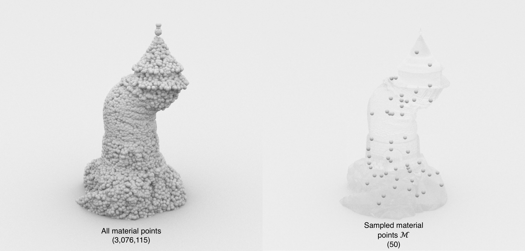
Figure 5 displays an example of the sample material point set from one of the experiments that will be discussed in Section 5.
3.2.2 Calculate full-space kinematics at quadrature points
To compute the dynamics of the sample material points , the equation of motion has to be integrated (13). We can discretize the spatial domain (14) with either Lagrangian quadrature points defined by the reference configuration or Eulerian quadrature points defined by the current configuration. Consequently, in the process of numerically evaluating the integral (15), we can use a quadrature rule defined either on the Lagrangian quadrature points or the Eulerian quadrature points. Note that the original MPM algorithm adopts the Lagrangian quadrature approach where the material points serve as the Lagrangian quadrature points.
Formally, we can discretize the weak form (13) using quadrature points:
| (27) |
where denotes the number of the quadrature points and the left superscript indicates quantities related to the quadrature points. Note that Eq. (27) generalizes Eq. (15) from the original material point method to allow for hyper-reduction and alternative quadrature rules.
3.2.2.1 Quadrature points via Lagrangian material points
The first approach is similar to that employed by the original MPM algorithm. Here, we use the neighboring material points to define the quadrature rule (Figure 6 left). Formally, we consider the neighbors of the sample material points , which we define as the subset of all material points that share Eulerian basis-function support with the sample material points (with ). Together, the sample material points and the neighboring material points form the set of the quadrature points, i.e., , , where and is a bijective mapping between the two sets.
Algorithm 3 provides the algorithm that identifies these quadrature points and obtains their kinematic information from the approximated deformation map.
This approach is most similar to the original emulated MPM approach, and it can incur an operation count independent of the original number of material points and Eulerian basis functions . However, it does require computing (and tracking) the set of neighboring material points. In the worst case, tracking would result in -dependent complexity due to the difficulty of ascertaining a priori the set of neighboring material points that will ever be encountered for a targeted sample point for any possible online trajectory.
3.2.2.2 Quadrature points via Eulerian quadrature points
To avoid the costly tracking of these neighboring material points, we present an alternative that generates Eulerian quadrature points instead of the Lagrangian quadrature points (Figure 6 right). The resulting quadrature rules discretize the Eulerian configuration instead of the Lagrangian configuration. We generate quadrature points per dimension and per background grid cell. These quadrature point locations are evenly distributed such that the distance between each pair of neighboring quadrature point is , where is the grid-cell width. Therefore, for each quadrature point, we have its current position and its volume , where denotes the volume of the grid cell.
To compute the undeformed position of the Eulerian quadrature points in the reference configuration, we can invert the approximated deformation by computing such that . Other kinematic quantities can then be computed using Equation 21 and Equation 22. The mass of each quadrature point can be computed as . These Eulerian quadrature points can then be used the same way as the Lagrangian quadrature points to discretize the weak form of the equation of motion (27).
Algorithm 4 presents the associated algorithm. In contrast to the first approach, this approach does not require tracking any neighboring material points. Instead, leveraging the invertibility of the deformation map, we can generate quadrature points necessary for updating the dynamics of the sample material points. Consequently, the approach can incur an operation count independent of the original number of material points and Eulerian basis functions without any additional tracking.
Remark.
In addition to reducing the computational cost, the ability to generate arbitrary quadratures also enables adaptive refinement, which can be instrumental when there is extreme deformation (i.e., the determinant of the deformation gradient is large).
Remark.
Since this work considers only elasticity, the quadrature points do not carry internal state variables; for plasticity, we will need to equip the approach with a mechanism to predict (continuous) fields of internal state variables. These fields could also be pursued with the mesh-independent low-dimensional manifold presented in Section 3.1.
3.2.3 Calculate the full-space dynamics
This section calculates the full-space dynamics by computing the trial velocities and positions for the material points belonging to the subset at . We deem these velocities and positions trial because they do not necessarily respect the kinematic constraint (19) induced by the low-dimensional manifold; they are simply the updates to the velocities and positions that would be computed from the current state by the full-order model, restricted to the set of sample material points. Algorithm 5 presents the MPM-style dynamics calculation that works for both the Lagrangian-quadrature kinematics and the Eulerian-quadrature kinematics.
Remark.
A salient difference between the original MPM algorithm (Algorithm 1) and the dynamics calculation presented here is that this new approach no longer needs to evolve the deformation gradient explicitly. The deformation gradient is readily available from the approximated deformation map’s spatial gradient as derived in Eq. (21).
3.2.4 Calculate the reduced-space dynamics
This section proposes two approaches for computing reduced-space dynamics that project the newly computed full-space trial positions and velocities onto the low-dimensional manifold, which effectively updates the generalized coordinates and velocity.
Algorithm 6 presents an approach that performs a least-squares projection of the symplectic Euler updated position and velocity onto the manifold and its tangent space, respectively. This associates with a least-squares projection of the position and velocity, where the least-squares problem is linear for the velocity, but nonlinear for the position; we solve the latter using the Gauss–Newton method [Nocedal and Wright 2006] with backtracking. We refer to this approach as the position-velocity projection scheme.
| (28) | |||
| (29) |
To reduce computational costs, we can linearize the nonlinear solve; Appendix A provides the derivation. The resulting approach is detailed in Algorithm 7. Since only velocity is involved in the least-squares projection, we refer to this projection scheme as the velocity-only projection scheme; in principle, it does not require the full-space trial positions , .
| (30) |
4 Manifold-parameterization construction via implicit neural representation
In principle, the manifold-parameterization function could be constructed in various ways. In this work, we employ a fully-connected deep-learning architecture (i.e., a multilayer perceptron) for this purpose (Figure 7), which yields an implicit neural representation of the deformation map. Recently in the the computer vision community, this particular network structure has been shown to successfully model the signed distance fields of various geometries [Park et al. 2019] and the radiance fields of different viewing directions [Mildenhall et al. 2020]. We adopt ELU activations to ensure continuous differentiability of the deformation-map approximation, which is needed to compute the deformation gradient and velocity as expressed in Eq. (21) and Eq. (22), respectively. As discussed in Section 3.1, the inputs to correspond to the undeformed position of a material point and the generalized coordinates , the latter of which is shared among all material points. The output of is the approximated deformed position of the material point . Thanks to the network’s continuous differentiability, we also obtain the approximated deformation gradient and approximated velocity via backpropagation.
4.1 Encoder
To train the manifold-parameterization function , we also need to define the value of the generalized coordinates at each time step for each training parameter instance . We do so implicitly by introducing an encoder network , which we train along with . is the input to , which is defined by concatenating the deformed positions of all the material points. Such an input encourages the injectivity of with respect to since there exists a unique that corresponds to a simulation state, as defined by all the positions of the material points. This input is particularly suitable for history-independent problems, e.g., elasticity. For history-dependent problems, history-dependent variables can also be concatenated to the input to the encoder function to define a simulation state uniquely. In practice, it is not essential that all material point positions are included in the input; a subset could be selected in purpose to keep training tractable with highly resolved training simulations. In addition, the encoder structure also encourages a spatially and temporally coherent representation of the simulation state where contiguous generalized coordinates correspond to nearby simulation states [Bengio et al. 2013].
Remark.
While we utilize a neural-network-based encoder to associate each training sample with a value for the generalized coordinates, this association can also be made in other ways. For example, the generalized coordinates for each training sample can be defined by explicit, manual choice or by exposing the generalized coordinates for each training sample to the optimization algorithm as training variables along with the network weights. In practice, we found these approaches challenging to scale to problems involving a large number of training samples, as the number of optimization variables with this approach scales linearly with the number of training samples. Furthermore, it is inconvenient to enforce spatial and temporal coherence with these techniques.
4.2 Loss function
We compute the neural-network weights and of the functions and as the (approximate) solutions to the minimization problem
| (31) | ||||
where , denotes the parameter instances for training, at which the full-order model has been solved and solutions are available, and denote penalty parameters for the deformation gradient and velocity, respectively.
The deformation-gradient penalty serves to enable the network to generate a manifold that can accurately represent the spatial gradients (Eq. (21)), which is essential for both Lagrangian-quadrature kinematics (Algorithm 3) and Eulerian-quadrature kinematics (Algorithm 4). The velocity penalty serves to enable the network to generate a manifold whose tangent space can accurately capture the velocity (Eq. (22)). This concept could be applied to higher-order spatiotemporal derivatives if desired. The practical choices of and are detailed in the result section (Section 5).
Note that the term is a finite difference approximation of the generalized velocity. Such an approximation mitigates the truncation error incurred by the linearization underpinning the velocity-only projection scheme for reduced-space dynamics (Appendix A).
5 Numerical experiments
We demonstrate the robustness of the proposed reduced-order approach on several large-deformation nonlinear elasticity problems with complex geometry. The particular constitutive law we adopt is the fixed corotated hyperelastic energy by Stomakhin et al. 2012; in principle, any hyperelastic model is compatible with the proposed approach without modification. We employ the open-source explicit MPM implementation by Wang et al. 2020a to define our baseline full-order model. Both the full-order and reduced-order models run on 12 threads on a 2.30GHz Intel Xeon E5-2686 v4 CPU. In addition, the neural network portion of the reduced-order model pipeline—which comprises evaluation, inversion, and differentiation of the deformation-map approximation—is implemented using the LibTorch library [Paszke et al. 2019] and runs on a single NVIDIA Tesla V100 GPU.
| Encoder network |
| 1D convolution layers |
| Layer | Kernel size | Stride size |
|---|---|---|
| Fully-connected layers |
| Layer | Input dimension | Output dimension |
|---|---|---|
| Manifold-parameterization function |
| Fully-connected layers |
| Layer | Input dimension | Output dimension |
| 1 | ||
| 2 | ||
| 3 | ||
| 4 | ||
| 5 |
Table 1 lists the detailed network structure of the manifold-parameterization function and the encoder function . We adopt this network structure for all experiments presented in this work. The rest of the training details are listed in Appendix B.
For hyper-reduction (Section 3.2.1), we find sampling at least 5 material points from each kinematic boundary generates stable reduced-order dynamics. For the Eulerian quadrature point scheme (Section 3.2.2), we use , i.e., 2 quadrature points per cell per dimension. For the position-velocity projection scheme (Section 3.2.4), we use a simple linear interpolation of the previous generalized coordinates as the initial guess, ), and the solver typically converges in 2–3 iterations.
All reported errors in the following sections correspond to the accumulated position errors (%) of the test simulations executed at parameter instances not included in the set employed for training, i.e.,
Here, with denotes the set of test parameter instances. Note that this approach to error estimation is not practical for real applications, as it requires executing the full-order model and evaluating the discrepancy between the full-order and reduced-order solutions for all material points at every time instance. Future work will pursue applying approaches that generate low-cost, statistically validated models of the ROM error Freno and Carlberg 2019, Parish and Carlberg 2020.
| Experiment | Geometry | Young’s | Poisson | # of | Grid cell | Particles per cell | Time step | Time steps | # of training | # of testing |
|---|---|---|---|---|---|---|---|---|---|---|
| modulus | ratio | particles | width | per dimension | size | per simulation | simulations | simulations | ||
| Section 5.1 | Cylinder | Pa | cm | 2 | s | 30 | 24 | 6 | ||
| Section 5.2 | Cuboid | Pa | cm | 2 | s | 30 | 29 | 7 | ||
| Section 5.3 | Cylinder | Pa | cm | 2 | s | 432 | 12 | 24 | ||
| Section 5.4 | Tower | Pa | cm | 3 | s | 80 | 16 | 4 |
5.1 Gravity

We conduct our first set of numerical experiments on an elastic cylinder with a radius of cm and a height of cm. Its material and discretization parameters are listed in Table 2. The elastic cylinder is attached to a vertical wall on one side and deforms under the influence of a downward gravity (Figure 8).
We consider the parameterized problem , where denotes the magnitude of the gravitational force. We generate training and testing data via uniform sampling of points in the interval m/s2. For each value of , we execute a simulation of time steps. Therefore, a total of simulation snapshots are generated, including the initial conditions. We then randomly split the dataset of simulations into an offline training dataset of 24 full simulations and an online testing dataset of 6 full simulations.
5.1.1 The effect of gradient penalties

In Figure 9, we study the influence of offline training parameters on the accuracy of the online reduced-order simulation. The dimension of the generalized coordinates is fixed to be 7; similar trends are observed for other generalized-coordinates dimensions. After training, we conduct reduced-order simulations using the four different combinations proposed in Section 3.2 and Algorithm 2. To isolate the source of error, we do not conduct hyper-reduction here.
Training with a nonzero value of the velocity-penalty parameter significantly improves the accuracy of the velocity-only projection technique of Algorithm 7 (Figure 9 c and d). By contrast, the position-velocity projection scheme of Algorithm 6 (Figure 9 a and b) is less sensitive to the choice of . Such observations hold for both the Lagrangian quadratures and the Eulerian quadratures. This numerical result aligns well with the theoretical analysis of linearization (Appendix A), because the velocity-only projection technique relies primarily on the accuracy of the velocity projection. Furthermore, training with a nonzero value of the deformation-gradient penalty improves all four algorithm combinations (Figure 9 a, b, c, and d), likely due to the fact that this penalty encourages better deformation-gradient approximations that are essential for defining the quadrature-point kinematics.
5.1.2 The effect of the generalized coordinates dimension
Figure 10 demonstrates the effect of the generalized coordinates dimension , which is a key hyperparameter of the network structure (Section 4). We train networks with different generalized coordinates dimensions while fixing to be 0.01 and to be 100. Afterward, the trained networks are tested for reduced-order simulations. In order to isolate the source of error, hyper-reduction is not applied. Figure 10 shows that the four different algorithm combinations from Algorithm 2 demonstrate the same trend: increasing the generalized coordinates dimension improves the simulation accuracy because the network has a larger manifold dimension.
5.1.3 The effect of hyper-reduction
Figure 11 reports the influence that the number of sample material points has on the accuracy of the reduced-order simulations. After the offline training with a setup of , , , we conduct online, reduced-order simulations with various numbers of sample material points. Notably, with just 10 sample material points, all four quadrature and projection combinations yield an error of less than 1%. In addition, using just 100 points delivers the same level of accuracy as no hyper-reduction, i.e., all 1,368 points’ dynamics are computed (Section 3.2.3) and used for projection onto the generalized coordinates (Section 3.2.4).
5.1.4 Hyperparameter summary
To summarize all the offline and online hyperparameter options, we plot all the choices together (Figure 12). Section 5.1.1, Section 5.1.2, and Section 5.1.3 each presents a “slice” of the hyperparameter study in Figure 12 in order to articulate the effect of a particular parameter.
As shown in Figure 12, independent of quadrature and projection combinations, training with a generalized-coordinate dimension of always yields a worse result, e.g., vs. , vs. . Therefore, the default training strategy should use . Unlike the position-velocity projection scheme (Figure 12 a and b), the velocity-only projection scheme (Figure 12 c and d) also consistently yields better result when training with a positive temporal gradient penalty , e.g. vs. , vs. . Therefore, the default training strategy should use a positive temporal gradient penalty, especially when using velocity-only projection. The spatial gradient penalty also improves simulation accuracy, as discussed in Section 5.1.1. Therefore, the default training strategy should also include the spatial gradient penalty term, though its significance is lesser than the other terms (Figure 12). With the training strategy mentioned earlier, all four reduced-order schemes achieve less than 1% error with just 10-100 sample material points. To obtain meaningful results, projection with just one point should be avoided as it can cause an error over .
Since this section focuses on small-scale experiments that serve to support an extensive parameter study; as such, the opportunity for wall-time speedup of the reduced-order method over the full-order method is diminished. Experiments in Section 5.4 will report wall-time speedups for higher-dimension problems.
5.2 Torsion and tension

We apply tension and torsion to an elastic, rectangular cuboid (Figure 13). The dimensions of the cuboid are cm, cm, and cm. Its material and discretization properties are listed in Table 2.
We consider the parameterized problem , where denotes the translational velocity and denotes the rotational velocity. We generate simulation data by varying the translational velocity ( m/s) and the rotational velocity ( rad/s). A total number of simulations are generated via full factorial sampling of the translation and the rotational velocities with six evenly spaced samples in each dimension, i.e., and . Each simulation consists of time steps. Therefore, we generate a total of simulation snapshots, including the initial conditions. Afterward, we randomly assign full simulations for training and for testing. Specifically, the testing parameters are and the rest are used for training.
| Scheme | Sample material | Sample material |
|---|---|---|
| points count: 50 | points count: 1,757 (all) | |
| Lagrangian quad + position-velocity proj | ||
| Lagrangian quad + velocity-only proj | ||
| Eulerian quad + position-velocity proj | ||
| Eulerian quad + velocity-only proj |
An approximated deformation map network is trained with (cf. Section 5.1.4). We then conduct reduced-order simulations using this network. Table 3 reports the testing errors of the reduced-order simulations using different quadrature and projection combinations with and without hyper-reduction, demonstrating the effectiveness of the reduced-order simulation in modeling tension and torsion.
5.2.1 Zero-shot super-resolution

| Scheme | Position error |
|---|---|
| Lagrangian quad + position-velocity proj | |
| Lagrangian quad + position-velocity proj (w/hyper-red) | |
| Lagrangian quad + velocity-only proj | |
| Lagrangian quad + velocity-only proj (w/hyper-red) | |
| Eulerian quad + position-velocity proj | |
| Eulerian quad + position-velocity proj (w/hyper-red) | |
| Eulerian quad + velocity-only proj | |
| Eulerian quad + velocity-only proj (w/hyper-red) | |
| Super-resolution baseline |
An advantage of training the deformation map instead of a finite number of material points is that we can easily adjust the resolution of the reduced-order simulation. We can infer the dynamics of an infinite number of material points so long as they belong to the reference domain. Consequently, even though the deformation map is trained on low-resolution simulations (Figure 14b), we can run high-resolution reduced-order simulations (Figure 14c) by using a finer MPM grid. Since the high-resolution simulation is never exposed to the training process, zero-shot super-resolution is achieved [Li et al. 2021b]. We construct a super-resolution baseline by advecting high-resolution material points on the velocity field computed by the low-resolution simulation (a), employing the popular “tracer particle technique” [Stam 1999, Fu et al. 2017]. Both simulations are compared with the high-resolution ground truth (Figure 14d). Table 4 lists the errors of the super-resolution simulations of all the reduced-order schemes and the baseline, across the entire testing dataset. All reduced-order methods outperform the super-resolution baseline significantly. Figure 14 demonstrates the visual superiority of our approach in comparison with the baseline approach.
5.3 Poke-and-recover

Poking is a frequent use case of the elasticity simulation where a force is applied in a particular direction at a small portion of the material and is released after a short period. The material then recovers to its undeformed state due to elasticity.
The elastic cylinder from Section 5.1 is poked at the top (Figure 15). The poking force is characterized by the spherical coordinate, where . The corresponding poking location, at which the force is applied, is , where and are the radius and the height of the cylinder, respectively. is chosen such that the poked location moves at a constant speed of 4.8 cm/s. is fixed to be . The poking force is applied for 0.25 s before it is released. After the force is released, the cylinder recovers to its initial state due to elasticity.
We consider the parameterized problem . We generate simulation data via uniform sampling of in with an interval of , yielding a total of simulations. We use of these simulations for training. The value of for these simulations is evenly spaced with an interval of . The remaining simulations are used for testing. The goal of this training and testing split is to gauge the ability of the proposed reduced-order model to respond to pokes at arbitrary values of . Each simulation consists of time steps. Therefore, a total of simulation snapshots, including the initial conditions, are used for training and testing.
| Scheme | Sample material | Sample material |
|---|---|---|
| points count: 50 | points count: 1,368 (all) | |
| Lagrangian quad + position-velocity proj | ||
| Lagrangian quad + velocity-only proj | ||
| Eulerian quad + position-velocity proj | ||
| Eulerian quad + velocity-only proj |
We first conduct offline training with (cf. Section 5.1.4) and then run online reduced-order simulations. Table 5 reports the testing errors of the reduced-order simulations using different quadrature and projection combinations with and without hyper-reduction, demonstrating the effectiveness of the reduced-order simulation in modeling the poke-and-recover problem.
5.3.1 Reduced-space trajectory
Figure 16 plots the trajectory of the generalized coordinates of a reduced poke-and-recover simulation. Since is high-dimensional in general, we visualize by projecting it onto a 2D plane spanned by its first two principal components.
Under the influence of the poking force, the material takes up a deformed state in the full space ; after the force is removed, the material then returns to its undeformed state. It is also desirable to maintain such a “return” property in the reduced space , where returns to its initial value. In general, one state in the full space can correspond to multiple generalized coordinates, i.e., the approximate deformation map is not necessarily injective with respect to . By using the encoder training scheme presented in Section 4.1, we can encourage injectivity and can indeed maintain the “return” property in the reduced space. As shown in Figure 16, the generalized coordinates return to the origin, which maps to the undeformed state in the full space.
5.3.2 Continual manipulation


One advantage of maintaining the “return” property is that even though the training data consists of simulations poking only once, we can actually run reduced-order simulations that poke repetitively. After each poke-and-recover sequence, the generalized coordinates return to their starting values, ready to be poked again in an arbitrary direction.
Therefore, we run a reduced-order simulation consisting of ten consecutive poke-and-recover sequences, where the poking direction is chosen each time randomly (Figure 17). This simulation has 4320 time steps or 30 s in total. Table 6 reports its error in comparison with the full-order simulation. All quadrature and projection combinations produce good agreements with and without hyper-reduction. Note that no full-order simulation of 30 s is included in the training data. All training simulations are 3 s, demonstrating our framework’s robust generalization capability. Our work also handles more complex geometries (Figure 18).
| Scheme | Sample material | Sample material |
|---|---|---|
| points count: 50 | points count: 1,368 (all) | |
| Lagrangian quad + position-velocity proj | ||
| Lagrangian quad + velocity-only proj | ||
| Eulerian quad + position-velocity proj | ||
| Eulerian quad + velocity-only proj |
5.4 Large-scale experiments

To demonstrate the efficiency of the reduced-order simulation in comparison to the full-order simulation, we conduct large-scale experiments with a complex tower geometry (Figure 19). The material and discretization parameters of the object are listed in Table 2. Table 7 details the data generation time and training time.
| Data generation time | Training time |
|---|---|
| s | s |
Both the top and the bottom of the object experiences Dirichlet boundary conditions. The top is kinematically moved under a fixed velocity while the bottom is stationary. The fixed velocity is parameterized by a spherical coordinate, , where , , and .
We analyze the proposed approach in this parametrized setting (). We generate training data by running 16 simulations with different triplets sampled using the Latin hypercube method [Stein 1987]. We further sample another simulations for testing purposes using the same approach.
An approximated deformation map network is trained with (cf. Section 5.1.4). Afterward, we conduct systematic tests over the different reduced-order approaches and different numbers of sample material points (Figure 20). All setups using the Eulerian quadratures (pentagon and cross) offer a significant speedup over the full-order model while maintaining accuracy. By contrast, due to their need to track every material point, Lagrangian quadrature approaches (circle and square) do not offer a reduction in computation complexity and do not offer speedup over the full-order model. While velocity-only projection methods (square and cross) generally have a slightly higher error than position-velocity projection methods (circle and pentagon), they are also computationally faster. Across all methods, the fewer sample material points, the faster the simulation and the higher the error. In particular, the reduced-order simulations employing Eulerian quadratures and velocity-only projection with fewer than 50 sample material points (blue cross and orange cross) attain real-time performance and are over 20 times faster than the baseline full-order model. Figure 19 displays all four testing simulations using the Eulerian quadratures and velocity-only projection with 50 sample material points (orange cross). Visually, the reduced-order simulations agree well with the full-order simulations while missing some secondary wrinkle deformations. Further research can be conducted on increasing the complexity of the network to capture these secondary deformations [Sitzmann et al. 2020, Takikawa et al. 2021].
Remark.
Instead of computing the dynamics of over 3 million material points, we only need to calculate the dynamics of no more than 50 points (over 600,000 times reduction). However, the speedup number we observe is reduced to 20X. This discrepancy can be understood by the nonlocal nature of MPM, where a neighborhood of quadratures points is required for computing the dynamics of even just one material point. Consequently, in order to update the dynamics of 50 points, over 20,000 quadrature points are involved in the particle to grid transfer. To achieve the full wall-clock performance potential of the reduced-order model, further research should consider adaptive quadrature rules that lower the total number of quadrature points involved.
Remark.
We adopt a random sampling approach for choosing hyper-reduction sample material points (Section 3.2.1). While such a method is easy to implement, it does not guarantee optimality in terms of errors and computation costs. Future work should be conducted to select the optimal set of hyper-reduction points to minimize the position error and the computation cost.
5.4.1 Comparison
To compare the proposed framework with other model reduction methods, we first notice that there is no prior work on model reduction of MPM using the classical approach (Figure 1a). As discussed in Section 1.3, the classical approach (e.g., POD) is unsuitable for model reduction of MPM due to the challenge of approximating the deformation gradients and achieving hyper-reduction. Consequently, we construct a baseline model using our approach (Figure 1b) with a linear manifold. Essentially, we replace the nonlinear manifold-parameterization function with a linear one. In practice, this amounts to replacing the multilayer neural-network-based manifold-parameterization function (Figure 7) with a single linear layer (without activation), wherein we train only the weights and biases of a single layer; as such, it is similar to classical linear-subspace methods such as POD. Note that the the nonlinear manifold and the linear manifold share the same reduced-dimension of .

As shown in Figure 21, our nonlinear manifold significantly outperforms the linear one in terms of training accuracy, both quantitatively and visually. The linear approximation struggles to reconstruct the highly nonlinear deformation of the elastic object. We further attempted to deploy the trained linear manifold in the same setting as Figure 20. However, simulations using the linear manifold all went unstable in just a few time steps and were unable to complete the simulation. This is somewhat anticipated since the projection-based dynamics (Section 3.2) further depend on the gradient information of the manifold-parameterization function. We thereby draw the conclusion that the robust, expressive nonlinear manifold (engineered via a deep neural network) proposed in this work is essential for building a manifold-parameterization function of the highly nonlinear deformation map.
6 Conclusions and future work
This work has presented—to our knowledge—the first projection-based reduced-order model for the material point method. In contrast with prior model reduction techniques that build a low-dimensional manifold of the discretization of the “deformation map”, we create a discretization-agnostic, continuously-differentiable, low-dimensional manifold of the “deformation map” itself based on implicit neural representations. We then utilize this low-dimensional manifold to drive the MPM simulation via optimal-projection-based dynamics, ensuring the simulated trajectory remains on the low-dimensional manifold associated with the deformation-map approximation. We propose two different quadrature approaches for computing full-space kinematics, and two different projection approaches for computing reduced-space dynamics. Through the introduction of hyper-reduction, we demonstrate that this approach can drastically reduce the dimension of the MPM hyperelasticity simulations and offers an order-of-magnitude wall-time speedup.
Moving forward, we envision 3 exciting directions to improve our work. (1) Supporting more continuum mechanics phenomena. We aim to extend our work to support other material behaviors, such as plasticity, fracture, contact, and collision. (2) Improving wall-time performance. This work focuses on the spatial model reduction of MPM. Future work should also consider a reduction in the temporal domain in order to take a larger time step size. Since the stress evaluation is completed on the CPU while the neural network evaluation is completed on the GPU, expensive CPU-GPU transfer is conducted at each time step. Future work might investigate a full GPU implementation to avoid the costly transfer. One may also consider expediting training time via more advanced data structures and optimization [Müller et al. 2022, Liu et al. 2020, Martel et al. 2021, Takikawa et al. 2021]. To improve training scalability, we can use hyperreduction samples as the input to the encoder instead of the full-order samples. (3) Extending the use of implicit neural representations in model reduction for other types of systems and discretization methods. Even though the proposed model reduction framework is designed for MPM, the proposed manifold parameterization function is, in fact, discretization independent. Therefore, we would like to go beyond MPM and explore its ability in model reduction of other continuum mechanics discretizations, such as the finite element method (FEM) and smoothed-particle hydrodynamics (SPH). For the same reason, we would also like to explore the manifold parameterization function’s ability to learn from simulation data with adaptive refinement.
Acknowledgements
We thank Henrique Teles Maia for proofreading the manuscript. This work was supported in part by the National Science Foundation (Grants CBET-17-06689 and CHS-1717178) as well as SideFX.
References
- Abgrall and Crisovan [2018] Abgrall, R., Crisovan, R., 2018. Model reduction using -norm minimization as an application to nonlinear hyperbolic problems. International Journal for Numerical Methods in Fluids 87, 628–651.
- Amsallem et al. [2009] Amsallem, D., Cortial, J., Carlberg, K., Farhat, C., 2009. A method for interpolating on manifolds structural dynamics reduced-order models. International journal for numerical methods in engineering 80, 1241–1258.
- Amsallem et al. [2012] Amsallem, D., Zahr, M.J., Farhat, C., 2012. Nonlinear model order reduction based on local reduced-order bases. International Journal for Numerical Methods in Engineering 92, 891–916.
- An et al. [2008] An, S.S., Kim, T., James, D.L., 2008. Optimizing cubature for efficient integration of subspace deformations. ACM transactions on graphics (TOG) 27, 1–10.
- Barbič and Zhao [2011] Barbič, J., Zhao, Y., 2011. Real-time large-deformation substructuring. ACM transactions on graphics (TOG) 30, 1–8.
- Bardenhagen et al. [1998] Bardenhagen, S., Brackbill, J., Sulsky, D., 1998. Shear deformation in granular materials. Technical Report. Los Alamos National Lab., NM (United States).
- Barone et al. [2009] Barone, M.F., Kalashnikova, I., Segalman, D.J., Thornquist, H.K., 2009. Stable galerkin reduced order models for linearized compressible flow. Journal of Computational Physics 228, 1932–1946.
- Baur et al. [2011] Baur, U., Beattie, C., Benner, P., Gugercin, S., 2011. Interpolatory projection methods for parameterized model reduction. SIAM Journal on Scientific Computing 33, 2489–2518.
- Bengio et al. [2013] Bengio, Y., Courville, A., Vincent, P., 2013. Representation learning: A review and new perspectives. IEEE transactions on pattern analysis and machine intelligence 35, 1798–1828.
- Benner et al. [2015a] Benner, P., Feng, L., Li, S., Zhang, Y., 2015a. Reduced-order modeling and rom-based optimization of batch chromatography, in: Numerical Mathematics and Advanced Applications-ENUMATH 2013. Springer, pp. 427–435.
- Benner et al. [2015b] Benner, P., Gugercin, S., Willcox, K., 2015b. A survey of projection-based model reduction methods for parametric dynamical systems. SIAM review 57, 483–531.
- Bergmann et al. [2009] Bergmann, M., Bruneau, C.H., Iollo, A., 2009. Enablers for robust POD models. Journal of Computational Physics 228, 516–538.
- Bergmann et al. [2005] Bergmann, M., Cordier, L., Brancher, J.P., 2005. Optimal rotary control of the cylinder wake using proper orthogonal decomposition reduced-order model. Physics of fluids 17, 097101.
- Bridson [2007] Bridson, R., 2007. Fast poisson disk sampling in arbitrary dimensions. SIGGRAPH sketches 10.
- Bruns and Benner [2015] Bruns, A., Benner, P., 2015. Parametric model order reduction of thermal models using the bilinear interpolatory rational krylov algorithm. Mathematical and Computer Modelling of Dynamical Systems 21, 103–129.
- Carlberg [2015] Carlberg, K., 2015. Adaptive h-refinement for reduced-order models. International Journal for Numerical Methods in Engineering 102, 1192–1210.
- Carlberg et al. [2017] Carlberg, K., Barone, M., Antil, H., 2017. Galerkin v. least-squares Petrov–Galerkin projection in nonlinear model reduction. Journal of Computational Physics 330, 693–734.
- Carlberg et al. [2011] Carlberg, K., Bou-Mosleh, C., Farhat, C., 2011. Efficient non-linear model reduction via a least-squares petrov–galerkin projection and compressive tensor approximations. International Journal for numerical methods in engineering 86, 155–181.
- Carlberg and Farhat [2011] Carlberg, K., Farhat, C., 2011. A low-cost, goal-oriented ‘compact proper orthogonal decomposition’basis for model reduction of static systems. International Journal for Numerical Methods in Engineering 86, 381–402.
- Carlberg et al. [2013] Carlberg, K., Farhat, C., Cortial, J., Amsallem, D., 2013. The GNAT method for nonlinear model reduction: effective implementation and application to computational fluid dynamics and turbulent flows. Journal of Computational Physics 242, 623–647.
- Carlberg et al. [2015] Carlberg, K., Tuminaro, R., Boggs, P., 2015. Preserving Lagrangian structure in nonlinear model reduction with application to structural dynamics. SIAM Journal on Scientific Computing 37, B153–B184.
- Chen et al. [2019] Chen, P.Y., Blutinger, J.D., Meijers, Y., Zheng, C., Grinspun, E., Lipson, H., 2019. Visual modeling of laser-induced dough browning. Journal of Food Engineering 243, 9–21.
- Chen et al. [2021] Chen, P.Y., Chantharayukhonthorn, M., Yue, Y., Grinspun, E., Kamrin, K., 2021. Hybrid discrete-continuum modeling of shear localization in granular media. Journal of the Mechanics and Physics of Solids 153, 104404.
- Chen and Zhang [2019] Chen, Z., Zhang, H., 2019. Learning implicit fields for generative shape modeling, in: Proceedings of the IEEE/CVF Conference on Computer Vision and Pattern Recognition, pp. 5939–5948.
- Craig Jr and Bampton [1968] Craig Jr, R.R., Bampton, M.C., 1968. Coupling of substructures for dynamic analyses. AIAA journal 6, 1313–1319.
- Daphalapurkar et al. [2007] Daphalapurkar, N.P., Lu, H., Coker, D., Komanduri, R., 2007. Simulation of dynamic crack growth using the generalized interpolation material point (gimp) method. International Journal of Fracture 143, 79–102.
- Daviet and Bertails-Descoubes [2016] Daviet, G., Bertails-Descoubes, F., 2016. A semi-implicit material point method for the continuum simulation of granular materials. ACM Transactions on Graphics (TOG) 35, 1–13.
- Dosovitskiy et al. [2015] Dosovitskiy, A., Tobias Springenberg, J., Brox, T., 2015. Learning to generate chairs with convolutional neural networks, in: Proceedings of the IEEE conference on computer vision and pattern recognition, pp. 1538–1546.
- Drohmann et al. [2012] Drohmann, M., Haasdonk, B., Ohlberger, M., 2012. Reduced basis approximation for nonlinear parametrized evolution equations based on empirical operator interpolation. SIAM Journal on Scientific Computing 34, A937–A969.
- Erichson et al. [2019] Erichson, N.B., Muehlebach, M., Mahoney, M.W., 2019. Physics-informed autoencoders for lyapunov-stable fluid flow prediction. arXiv preprint arXiv:1905.10866 .
- Everson and Sirovich [1995] Everson, R., Sirovich, L., 1995. Karhunen–loeve procedure for gappy data. JOSA A 12, 1657–1664.
- Fang et al. [2013] Fang, F., Pain, C., Navon, I., Elsheikh, A., Du, J., Xiao, D., 2013. Non-linear petrov–galerkin methods for reduced order hyperbolic equations and discontinuous finite element methods. Journal of Computational Physics 234, 540–559. URL: https://www.sciencedirect.com/science/article/pii/S0021999112006006, doi:https://doi.org/10.1016/j.jcp.2012.10.011.
- Fang et al. [2018] Fang, Y., Hu, Y., Hu, S.M., Jiang, C., 2018. A temporally adaptive material point method with regional time stepping, in: Computer graphics forum, Wiley Online Library. pp. 195–204.
- Fang et al. [2019] Fang, Y., Li, M., Gao, M., Jiang, C., 2019. Silly rubber: an implicit material point method for simulating non-equilibrated viscoelastic and elastoplastic solids. ACM Transactions on Graphics (TOG) 38, 1–13.
- Fang et al. [2020] Fang, Y., Qu, Z., Li, M., Zhang, X., Zhu, Y., Aanjaneya, M., Jiang, C., 2020. IQ-MPM: an interface quadrature material point method for non-sticky strongly two-way coupled nonlinear solids and fluids. ACM Transactions on Graphics (TOG) 39, 51–1.
- Fei et al. [2021] Fei, Y., Guo, Q., Wu, R., Huang, L., Gao, M., 2021. Revisiting integration in the material point method: a scheme for easier separation and less dissipation. ACM Transactions on Graphics (TOG) 40, 1–16.
- Freno and Carlberg [2019] Freno, B.A., Carlberg, K.T., 2019. Machine-learning error models for approximate solutions to parameterized systems of nonlinear equations. Computer Methods in Applied Mechanics and Engineering 348, 250–296.
- Fu et al. [2017] Fu, C., Guo, Q., Gast, T., Jiang, C., Teran, J., 2017. A polynomial particle-in-cell method. ACM Transactions on Graphics (TOG) 36, 1–12.
- Fulton et al. [2019] Fulton, L., Modi, V., Duvenaud, D., Levin, D.I., Jacobson, A., 2019. Latent-space dynamics for reduced deformable simulation, in: Computer graphics forum, Wiley Online Library. pp. 379–391.
- Galbally et al. [2010] Galbally, D., Fidkowski, K., Willcox, K., Ghattas, O., 2010. Non-linear model reduction for uncertainty quantification in large-scale inverse problems. International journal for numerical methods in engineering 81, 1581–1608.
- Gao [2018] Gao, M., 2018. Sparse Paged Grid and its Applications to Adaptivity and Material Point Method in Physics Based Simulations. The University of Wisconsin-Madison.
- Gao et al. [2018] Gao, M., Wang, X., Wu, K., Pradhana, A., Sifakis, E., Yuksel, C., Jiang, C., 2018. GPU optimization of material point methods. ACM Transactions on Graphics (TOG) 37, 1–12.
- Gast et al. [2015] Gast, T.F., Schroeder, C., Stomakhin, A., Jiang, C., Teran, J.M., 2015. Optimization integrator for large time steps. IEEE transactions on visualization and computer graphics 21, 1103–1115.
- Glorot and Bengio [2010] Glorot, X., Bengio, Y., 2010. Understanding the difficulty of training deep feedforward neural networks, in: Proceedings of the thirteenth international conference on artificial intelligence and statistics, JMLR Workshop and Conference Proceedings. pp. 249–256.
- Gu [2011] Gu, C., 2011. Model order reduction of nonlinear dynamical systems. University of California, Berkeley.
- Gugercin et al. [2008] Gugercin, S., Antoulas, A.C., Beattie, C., 2008. H_2 model reduction for large-scale linear dynamical systems. SIAM journal on matrix analysis and applications 30, 609–638.
- Hall et al. [2000] Hall, K.C., Thomas, J.P., Dowell, E.H., 2000. Proper orthogonal decomposition technique for transonic unsteady aerodynamic flows. AIAA journal 38, 1853–1862.
- Han et al. [2019] Han, X., Gast, T.F., Guo, Q., Wang, S., Jiang, C., Teran, J., 2019. A hybrid material point method for frictional contact with diverse materials. Proceedings of the ACM on Computer Graphics and Interactive Techniques 2, 1–24.
- Hartman and Mestha [2017] Hartman, D., Mestha, L.K., 2017. A deep learning framework for model reduction of dynamical systems, in: 2017 IEEE Conference on Control Technology and Applications (CCTA), pp. 1917–1922. doi:10.1109/CCTA.2017.8062736.
- Holmes et al. [2012] Holmes, P., Lumley, J.L., Berkooz, G., Rowley, C.W., 2012. Turbulence, coherent structures, dynamical systems and symmetry. Cambridge university press.
- Holzapfel [2002] Holzapfel, G.A., 2002. Nonlinear solid mechanics: a continuum approach for engineering science. Meccanica 37, 489–490.
- Hu et al. [2019a] Hu, Y., Anderson, L., Li, T.M., Sun, Q., Carr, N., Ragan-Kelley, J., Durand, F., 2019a. Difftaichi: Differentiable programming for physical simulation. arXiv preprint arXiv:1910.00935 .
- Hu et al. [2018] Hu, Y., Fang, Y., Ge, Z., Qu, Z., Zhu, Y., Pradhana, A., Jiang, C., 2018. A moving least squares material point method with displacement discontinuity and two-way rigid body coupling. ACM Transactions on Graphics (TOG) 37, 1–14.
- Hu et al. [2019b] Hu, Y., Li, T.M., Anderson, L., Ragan-Kelley, J., Durand, F., 2019b. Taichi: a language for high-performance computation on spatially sparse data structures. ACM Transactions on Graphics (TOG) 38, 1–16.
- Hu et al. [2019c] Hu, Y., Liu, J., Spielberg, A., Tenenbaum, J.B., Freeman, W.T., Wu, J., Rus, D., Matusik, W., 2019c. Chainqueen: A real-time differentiable physical simulator for soft robotics, in: 2019 International conference on robotics and automation (ICRA), IEEE. pp. 6265–6271.
- Hu et al. [2021] Hu, Y., Liu, J., Yang, X., Xu, M., Kuang, Y., Xu, W., Dai, Q., Freeman, W.T., Durand, F., 2021. Quantaichi: a compiler for quantized simulations. ACM Transactions on Graphics (TOG) 40, 1–16.
- Hu et al. [2019d] Hu, Y., Zhang, X., Gao, M., Jiang, C., 2019d. On hybrid lagrangian-eulerian simulation methods: practical notes and high-performance aspects, in: ACM SIGGRAPH 2019 Courses, pp. 1–246.
- James et al. [2006] James, D.L., Barbič, J., Pai, D.K., 2006. Precomputed acoustic transfer: output-sensitive, accurate sound generation for geometrically complex vibration sources. ACM Transactions on Graphics (TOG) 25, 987–995.
- Jiang et al. [2017] Jiang, C., Gast, T., Teran, J., 2017. Anisotropic elastoplasticity for cloth, knit and hair frictional contact. ACM Transactions on Graphics (TOG) 36, 1–14.
- Jiang et al. [2015] Jiang, C., Schroeder, C., Selle, A., Teran, J., Stomakhin, A., 2015. The affine particle-in-cell method. ACM Transactions on Graphics (TOG) 34, 1–10.
- Jiang et al. [2016] Jiang, C., Schroeder, C., Teran, J., Stomakhin, A., Selle, A., 2016. The material point method for simulating continuum materials, in: ACM SIGGRAPH 2016 Courses, pp. 1–52.
- Jiang et al. [2020] Jiang, Y., Li, M., Jiang, C., Alonso-Marroquin, F., 2020. A hybrid material-point spheropolygon-element method for solid and granular material interaction. International Journal for Numerical Methods in Engineering 121, 3021–3047.
- Kashima [2016] Kashima, K., 2016. Nonlinear model reduction by deep autoencoder of noise response data, in: 2016 IEEE 55th Conference on Decision and Control (CDC), pp. 5750–5755. doi:10.1109/CDC.2016.7799153.
- Kim et al. [2019] Kim, B., Azevedo, V.C., Thuerey, N., Kim, T., Gross, M., Solenthaler, B., 2019. Deep fluids: A generative network for parameterized fluid simulations, in: Computer Graphics Forum, Wiley Online Library. pp. 59–70.
- Klár et al. [2016] Klár, G., Gast, T., Pradhana, A., Fu, C., Schroeder, C., Jiang, C., Teran, J., 2016. Drucker-prager elastoplasticity for sand animation. ACM Transactions on Graphics (TOG) 35, 1–12.
- Lall et al. [2002] Lall, S., Marsden, J.E., Glavaški, S., 2002. A subspace approach to balanced truncation for model reduction of nonlinear control systems. International Journal of Robust and Nonlinear Control: IFAC-Affiliated Journal 12, 519–535.
- Lee and Carlberg [2021] Lee, K., Carlberg, K., 2021. Deep conservation: A latent dynamics model for exact satisfaction of physical conservation laws, in: Proceedings of the AAAI Conference on Artificial Intelligence, pp. 277–285.
- Lee and Carlberg [2020] Lee, K., Carlberg, K.T., 2020. Model reduction of dynamical systems on nonlinear manifolds using deep convolutional autoencoders. Journal of Computational Physics 404, 108973.
- Li and Liu [2002] Li, S., Liu, W.K., 2002. Meshfree and particle methods and their applications. Appl. Mech. Rev. 55, 1–34.
- Li et al. [2020] Li, X., McWilliams, J., Li, M., Sung, C., Jiang, C., 2020. Soft hybrid aerial vehicle via bistable mechanism. arXiv preprint arXiv:2011.00426 .
- Li et al. [2021a] Li, Y., Li, X., Li, M., Zhu, Y., Zhu, B., Jiang, C., 2021a. Lagrangian–Eulerian multidensity topology optimization with the material point method. International Journal for Numerical Methods in Engineering 122, 3400–3424.
- Li et al. [2021b] Li, Z., Kovachki, N.B., Azizzadenesheli, K., liu, B., Bhattacharya, K., Stuart, A., Anandkumar, A., 2021b. Fourier neural operator for parametric partial differential equations, in: International Conference on Learning Representations. URL: https://openreview.net/forum?id=c8P9NQVtmnO.
- Lieu et al. [2006] Lieu, T., Farhat, C., Lesoinne, M., 2006. Reduced-order fluid/structure modeling of a complete aircraft configuration. Computer methods in applied mechanics and engineering 195, 5730–5742.
- Liu et al. [2020] Liu, L., Gu, J., Zaw Lin, K., Chua, T.S., Theobalt, C., 2020. Neural sparse voxel fields. Advances in Neural Information Processing Systems 33, 15651–15663.
- Lusch et al. [2018] Lusch, B., Kutz, J.N., Brunton, S.L., 2018. Deep learning for universal linear embeddings of nonlinear dynamics. Nature communications 9, 4950.
- Mainini and Willcox [2015] Mainini, L., Willcox, K., 2015. Surrogate modeling approach to support real-time structural assessment and decision making. AIAA Journal 53, 1612–1626.
- Martel et al. [2021] Martel, J.N., Lindell, D.B., Lin, C.Z., Chan, E.R., Monteiro, M., Wetzstein, G., 2021. ACORN: Adaptive coordinate networks for neural scene representation. arXiv preprint arXiv:2105.02788 .
- Martin et al. [2015] Martin, T., Umetani, N., Bickel, B., 2015. OmniAD: Data-driven omni-directional aerodynamics. ACM Transactions on Graphics (TOG) 34, 1–12.
- Mast et al. [2014] Mast, C.M., Arduino, P., Miller, G.R., Mackenzie-Helnwein, P., 2014. Avalanche and landslide simulation using the material point method: flow dynamics and force interaction with structures. Computational Geosciences 18, 817–830.
- Maulik et al. [2021] Maulik, R., Lusch, B., Balaprakash, P., 2021. Reduced-order modeling of advection-dominated systems with recurrent neural networks and convolutional autoencoders. Physics of Fluids 33, 037106.
- Maulik et al. [2020] Maulik, R., Mohan, A., Lusch, B., Madireddy, S., Balaprakash, P., Livescu, D., 2020. Time-series learning of latent-space dynamics for reduced-order model closure. Physica D: Nonlinear Phenomena 405, 132368.
- Mescheder et al. [2019] Mescheder, L., Oechsle, M., Niemeyer, M., Nowozin, S., Geiger, A., 2019. Occupancy networks: Learning 3d reconstruction in function space, in: Proceedings of the IEEE/CVF Conference on Computer Vision and Pattern Recognition, pp. 4460–4470.
- Mildenhall et al. [2020] Mildenhall, B., Srinivasan, P.P., Tancik, M., Barron, J.T., Ramamoorthi, R., Ng, R., 2020. NeRF: Representing scenes as neural radiance fields for view synthesis, in: European conference on computer vision, Springer. pp. 405–421.
- Moore [1981] Moore, B., 1981. Principal component analysis in linear systems: Controllability, observability, and model reduction. IEEE Transactions on Automatic Control 26, 17–32. URL: https://www.scopus.com/inward/record.uri?eid=2-s2.0-0019533482&doi=10.1109%2fTAC.1981.1102568&partnerID=40&md5=23f83f786523f08268214845f6cb25c8, doi:10.1109/TAC.1981.1102568. cited By 3526.
- Morton et al. [2018] Morton, J., Jameson, A., Kochenderfer, M.J., Witherden, F., 2018. Deep dynamical modeling and control of unsteady fluid flows, in: Advances in Neural Information Processing Systems, pp. 9258–9268.
- Müller et al. [2022] Müller, T., Evans, A., Schied, C., Keller, A., 2022. Instant neural graphics primitives with a multiresolution hash encoding. arXiv preprint arXiv:2201.05989 .
- Nairn [2003] Nairn, J.A., 2003. Material point method calculations with explicit cracks. Computer Modeling in Engineering and Sciences 4, 649–664.
- Nguyen and Peraire [2008] Nguyen, N.C., Peraire, J., 2008. An efficient reduced-order modeling approach for non-linear parametrized partial differential equations. International Journal for Numerical Methods in Engineering 76, 27–55.
- Nicolini et al. [2019] Nicolini, J.L., Na, D.Y., Teixeira, F.L., 2019. Model order reduction of electromagnetic particle-in-cell kinetic plasma simulations via proper orthogonal decomposition. IEEE Transactions on Plasma Science 47, 5239–5250.
- Nocedal and Wright [2006] Nocedal, J., Wright, S., 2006. Numerical optimization. Springer Science & Business Media.
- Otto and Rowley [2019] Otto, S.E., Rowley, C.W., 2019. Linearly recurrent autoencoder networks for learning dynamics. SIAM Journal on Applied Dynamical Systems 18, 558–593.
- Pan et al. [2023] Pan, S., Brunton, S.L., Kutz, J.N., 2023. Neural implicit flow: a mesh-agnostic dimensionality reduction paradigm of spatio-temporal data. Journal of Machine Learning Research 24, 1–60. URL: http://jmlr.org/papers/v24/22-0365.html.
- Parish and Carlberg [2020] Parish, E.J., Carlberg, K.T., 2020. Time-series machine-learning error models for approximate solutions to parameterized dynamical systems. Computer Methods in Applied Mechanics and Engineering 365, 112990.
- Park et al. [2019] Park, J.J., Florence, P., Straub, J., Newcombe, R., Lovegrove, S., 2019. DeepSDF: Learning continuous signed distance functions for shape representation, in: Proceedings of the IEEE/CVF Conference on Computer Vision and Pattern Recognition, pp. 165–174.
- Paszke et al. [2019] Paszke, A., Gross, S., Massa, F., Lerer, A., Bradbury, J., Chanan, G., Killeen, T., Lin, Z., Gimelshein, N., Antiga, L., et al., 2019. PyTorch: An imperative style, high-performance deep learning library. Advances in neural information processing systems 32, 8026–8037.
- Patankar and Joseph [2001] Patankar, N., Joseph, D., 2001. Lagrangian numerical simulation of particulate flows. International Journal of Multiphase Flow 27, 1685–1706.
- Peherstorfer and Willcox [2015] Peherstorfer, B., Willcox, K., 2015. Online adaptive model reduction for nonlinear systems via low-rank updates. SIAM Journal on Scientific Computing 37, A2123–A2150.
- Prud’homme et al. [2002] Prud’homme, C., Rovas, D., Veroy, K., Machiels, L., Maday, Y., Patera, A., Turinici, G., 2002. Reliable real-time solution of parametrized partial differential equations: Reduced-basis output bound methods. Journal of Fluids Engineering, Transactions of the ASME 124, 70–80. URL: https://www.scopus.com/inward/record.uri?eid=2-s2.0-0003321083&doi=10.1115%2f1.1448332&partnerID=40&md5=29f1d03ad99030052a1d54c28212f5a4, doi:10.1115/1.1448332. cited By 338.
- Raissi et al. [2019] Raissi, M., Perdikaris, P., Karniadakis, G.E., 2019. Physics-informed neural networks: A deep learning framework for solving forward and inverse problems involving nonlinear partial differential equations. Journal of Computational Physics 378, 686–707.
- Ram et al. [2015] Ram, D., Gast, T., Jiang, C., Schroeder, C., Stomakhin, A., Teran, J., Kavehpour, P., 2015. A material point method for viscoelastic fluids, foams and sponges, in: Proceedings of the 14th ACM SIGGRAPH/Eurographics Symposium on Computer Animation, pp. 157–163.
- Rathinam and Petzold [2003] Rathinam, M., Petzold, L.R., 2003. A new look at proper orthogonal decomposition. SIAM Journal on Numerical Analysis 41, 1893–1925.
- Regazzoni et al. [2019] Regazzoni, F., Dede, L., Quarteroni, A., 2019. Machine learning for fast and reliable solution of time-dependent differential equations. Journal of Computational physics 397, 108852.
- Romero et al. [2021] Romero, C., Casas, D., Pérez, J., Otaduy, M., 2021. Learning contact corrections for handle-based subspace dynamics. ACM Transactions on Graphics (TOG) 40, 1–12.
- Rowley [2005] Rowley, C.W., 2005. Model reduction for fluids, using balanced proper orthogonal decomposition. International Journal of Bifurcation and Chaos 15, 997–1013.
- Rozza et al. [2007] Rozza, G., Huynh, D., Patera, A., 2007. Reduced basis approximation and a posteriori error estimation for affinely parametrized elliptic coercive partial differential equations. Arch. Comput. Methods Eng. 15, 1–47. Cited By 27.
- Ryckelynck [2005] Ryckelynck, D., 2005. A priori hyperreduction method: an adaptive approach. Journal of computational physics 202, 346–366.
- Sadeghirad et al. [2011] Sadeghirad, A., Brannon, R.M., Burghardt, J., 2011. A convected particle domain interpolation technique to extend applicability of the material point method for problems involving massive deformations. International Journal for numerical methods in Engineering 86, 1435–1456.
- Sanchez-Gonzalez et al. [2020] Sanchez-Gonzalez, A., Godwin, J., Pfaff, T., Ying, R., Leskovec, J., Battaglia, P., 2020. Learning to simulate complex physics with graph networks, in: International Conference on Machine Learning, PMLR. pp. 8459–8468.
- Schulz et al. [2017] Schulz, A., Xu, J., Zhu, B., Zheng, C., Grinspun, E., Matusik, W., 2017. Interactive design space exploration and optimization for CAD models. ACM Transactions on Graphics (TOG) 36, 1–14.
- Shen et al. [2021] Shen, S., Yin, Y., Shao, T., Wang, H., Jiang, C., Lan, L., Zhou, K., 2021. High-order differentiable autoencoder for nonlinear model reduction. arXiv preprint arXiv:2102.11026 .
- Sirisup and Karniadakis [2004] Sirisup, S., Karniadakis, G., 2004. A spectral viscosity method for correcting the long-term behavior of POD models. Journal of Computational Physics 194, 92–116. URL: https://www.sciencedirect.com/science/article/pii/S0021999103004625, doi:https://doi.org/10.1016/j.jcp.2003.08.021.
- Sirovich [1987] Sirovich, L., 1987. Turbulence and the dynamics of coherent structures. iii. dynamics and scaling. Quarterly of Applied mathematics 45, 583–590.
- Sitzmann et al. [2020] Sitzmann, V., Martel, J., Bergman, A., Lindell, D., Wetzstein, G., 2020. Implicit neural representations with periodic activation functions. Advances in Neural Information Processing Systems 33.
- Stam [1999] Stam, J., 1999. Stable fluids, in: Proceedings of the 26th annual conference on Computer graphics and interactive techniques, pp. 121–128.
- Stein [1987] Stein, M., 1987. Large sample properties of simulations using latin hypercube sampling. Technometrics 29, 143–151.
- Stomakhin et al. [2012] Stomakhin, A., Howes, R., Schroeder, C., Teran, J.M., 2012. Energetically consistent invertible elasticity, in: Proceedings of the 11th ACM SIGGRAPH/Eurographics conference on Computer Animation, pp. 25–32.
- Stomakhin et al. [2013] Stomakhin, A., Schroeder, C., Chai, L., Teran, J., Selle, A., 2013. A material point method for snow simulation. ACM Transactions on Graphics (TOG) 32, 1–10.
- Stomakhin et al. [2014] Stomakhin, A., Schroeder, C., Jiang, C., Chai, L., Teran, J., Selle, A., 2014. Augmented MPM for phase-change and varied materials. ACM Transactions on Graphics (TOG) 33, 1–11.
- Su et al. [2021] Su, H., Xue, T., Han, C., Jiang, C., Aanjaneya, M., 2021. A unified second-order accurate in time mpm formulation for simulating viscoelastic liquids with phase change. ACM Transactions on Graphics (TOG) 40, 1–18.
- Sulsky et al. [1995] Sulsky, D., Zhou, S.J., Schreyer, H.L., 1995. Application of a particle-in-cell method to solid mechanics. Computer physics communications 87, 236–252.
- Takeishi et al. [2017] Takeishi, N., Kawahara, Y., Yairi, T., 2017. Learning Koopman invariant subspaces for dynamic mode decomposition, in: Advances in Neural Information Processing Systems, pp. 1130–1140.
- Takikawa et al. [2021] Takikawa, T., Litalien, J., Yin, K., Kreis, K., Loop, C., Nowrouzezahrai, D., Jacobson, A., McGuire, M., Fidler, S., 2021. Neural geometric level of detail: Real-time rendering with implicit 3d shapes, in: Proceedings of the IEEE/CVF Conference on Computer Vision and Pattern Recognition, pp. 11358–11367.
- Tan et al. [2020] Tan, Q., Pan, Z., Gao, L., Manocha, D., 2020. Realtime simulation of thin-shell deformable materials using CNN-based mesh embedding. IEEE Robotics and Automation Letters 5, 2325–2332.
- Umetani et al. [2014] Umetani, N., Koyama, Y., Schmidt, R., Igarashi, T., 2014. Pteromys: Interactive design and optimization of free-formed free-flight model airplanes. ACM Transactions on Graphics (TOG) 33, 1–10.
- Wang et al. [2019] Wang, S., Ding, M., Gast, T.F., Zhu, L., Gagniere, S., Jiang, C., Teran, J.M., 2019. Simulation and visualization of ductile fracture with the material point method. Proceedings of the ACM on Computer Graphics and Interactive Techniques 2, 1–20.
- Wang et al. [2020a] Wang, X., Li, M., Fang, Y., Zhang, X., Gao, M., Tang, M., Kaufman, D.M., Jiang, C., 2020a. Hierarchical optimization time integration for CFL-rate MPM stepping. ACM Transactions on Graphics (TOG) 39, 1–16.
- Wang et al. [2020b] Wang, X., Qiu, Y., Slattery, S.R., Fang, Y., Li, M., Zhu, S.C., Zhu, Y., Tang, M., Manocha, D., Jiang, C., 2020b. A massively parallel and scalable multi-GPU material point method. ACM Transactions on Graphics (TOG) 39, 30–1.
- Wang et al. [2012] Wang, Z., Akhtar, I., Borggaard, J., Iliescu, T., 2012. Proper orthogonal decomposition closure models for turbulent flows: a numerical comparison. Computer Methods in Applied Mechanics and Engineering 237, 10–26.
- Więckowski et al. [1999] Więckowski, Z., Youn, S.K., Yeon, J.H., 1999. A particle-in-cell solution to the silo discharging problem. International journal for numerical methods in engineering 45, 1203–1225.
- Wiewel et al. [2019] Wiewel, S., Becher, M., Thuerey, N., 2019. Latent space physics: Towards learning the temporal evolution of fluid flow, in: Computer graphics forum, Wiley Online Library. pp. 71–82.
- Willcox and Peraire [2002] Willcox, K., Peraire, J., 2002. Balanced model reduction via the proper orthogonal decomposition. AIAA journal 40, 2323–2330.
- Wolper et al. [2019] Wolper, J., Fang, Y., Li, M., Lu, J., Gao, M., Jiang, C., 2019. CD-MPM: continuum damage material point methods for dynamic fracture animation. ACM Transactions on Graphics (TOG) 38, 1–15.
- Yang et al. [2015] Yang, Y., Li, D., Xu, W., Tian, Y., Zheng, C., 2015. Expediting precomputation for reduced deformable simulation. ACM Trans. Graph 34.
- York et al. [2000] York, A.R., Sulsky, D., Schreyer, H.L., 2000. Fluid–membrane interaction based on the material point method. International Journal for Numerical Methods in Engineering 48, 901–924.
- Yue et al. [2015] Yue, Y., Smith, B., Batty, C., Zheng, C., Grinspun, E., 2015. Continuum foam: A material point method for shear-dependent flows. ACM Transactions on Graphics (TOG) 34, 1–20.
- Yue et al. [2018] Yue, Y., Smith, B., Chen, P.Y., Chantharayukhonthorn, M., Kamrin, K., Grinspun, E., 2018. Hybrid grains: adaptive coupling of discrete and continuum simulations of granular media. ACM Transactions on Graphics (TOG) 37, 1–19.
A Projection linearization
Substituting into Equation 29 yields
| (32) |
Using Taylor’s theorem, we have
Under this linearization, Equation 32 becomes Equation 30. Consequently, the effectiveness of velocity-only projection depends on the accuracy of such a linearization.
B Training details
We implement the network in PyTorch [Paszke et al. 2019] and train the network with the ADAM optimizer with an adaptive learning rate, decreasing from to . We initialize the neural network’s weights using the Xavier initialization [Glorot and Bengio 2010]. We conduct standard feature-scaling for the network’s input and output to ease the training process. Min-max normalization is performed for the reference positions, while standardization is conducted for the network’s output to have zero mean and unit variance.