Cosmological Dynamics of Cuscuta-Galileon Gravity

Sirachak Panpanich Email: sirachakp-at-aoni.waseda.jp Address: Department of Pure and Applied Physics, Graduate School of Advanced Science and Engineering, Waseda University, Okubo 3-4-1, Shinjuku, Tokyo 169-8555, Japan Kei-ichi Maeda Email: maeda-at-waseda.jp Address: Department of Pure and Applied Physics, Graduate School of Advanced Science and Engineering, Waseda University, Okubo 3-4-1, Shinjuku, Tokyo 169-8555, Japan

August 11, 2026

Abstract

We study cosmological dynamics of the cuscuta-galileon gravity with a potential term by using the dynamical system approach. This model is galileon generalization of the cuscuton gravity where we add a potential term to the theory in order to obtain the radiation and matter dominated eras. The exponential potential can provide the sequence of the thermal history of the Universe correctly, i.e. starting from radiation dominance, passing through matter dominant era, and then approaching de Sitter expansion stage. This model has no ghosts and the Laplacian instability for both scalar and tensor perturbations. We also discuss the observational constraints on the model parameters. It turns out that the model actually has three degrees of freedom unlike the original cuscuton theory.

I Introduction

Many modified gravity models require additional degrees of freedom (d.o.f.) besides two tensor gravitational degrees of freedom to explain an accelerated expansion of the Universe Riess:1998cb; Perlmutter:1998np. For example, Horndeski theories Horndeski:1974wa; Deffayet:2011gz; Kobayashi:2011nu using a scalar field have three d.o.f., generalized Proca theories Heisenberg:2014rta using a vector field have five d.o.f., and massive gravity using a massive tensor field has five d.o.f in the case of de Rham-Gabadadze-Tolley massive gravity deRham:2010ik; deRham:2010kj. However, until now, a fifth force or deviation from General Relativity in the solar system scale has not been detected Will:2014kxa. Therefore, they require screening mechanisms to hide their additional degrees of freedom Khoury:2003aq; Khoury:2003rn; Hinterbichler:2010es; Brax:2010gi; Burrage:2014uwa; Panpanich:2019rij; Brax:2012jr; Babichev:2009ee; Babichev:2013usa; Vainshtein:1972sx; Nicolis:2008in.

Recently there is development on modification of the gravitational theories which propagate only two gravitational degrees of freedom. The cuscuton gravity model was first proposed in Afshordi:2006ad; Afshordi:2007yx; Afshordi:2009tt, which can be regarded as the low-energy Horava-Lifshitz theoryAfshordi:2009tt. Some extension was also found in minimally modified gravity (MMG) Lin:2017oow; Aoki:2018zcv; Aoki:2018brq; Mukohyama:2019unx; DeFelice:2020eju; Aoki:2020oqc and extended cuscuton gravity Iyonaga:2018vnu; Iyonaga:2020bmm. The minimally modified gravity is a construction of Hamiltonian of the gravitational theory which provides only two d.o.f., while the extended cuscuton is a generalization of an original cuscuton theory in the context of the beyond Horndeski theories Gleyzes:2014dya. In these models the scalar field turns out to be nondynamical because either the second-order time derivatives of a scalar field are absent in the equations of motion (MMG), or we can eliminate them after linear combination of the equations of motion and the Friedmann equation (extended cuscuton).

Besides above two classes of theories, the cuscuta-galileon gravity which is a simple galileon generalization of the original cuscuton gravity, was proposed deRham:2016ged. In the original cuscuton gravity, there exists a caustic singularity, which shows lacking predictability. Hence adding a galileon-like kinetic term in the original cuscuton theory, they discuss a simple extended model (the cuscuta-galileon theory), which can avoid the formation of caustic singularities in flat space-time deRham:2016ged.

In this work we investigate cosmological dynamics of the cuscuta-galileon gravity. We include a potential term because without a potential term, such a model does not provide a viable cosmological model just as the same as the original cuscuton theory Afshordi:2006ad; Afshordi:2007yx. In fact we find that radiation dominant and matter dominant eras do not exist as we will show in Appendix A. In the original cuscuton theory, adding a quadratic potential, we obtain the $\Lambda$ CDM model. Therefore, we imitate this idea by adding a potential term to the cuscuta-galileon action, and then investigate cosmological dynamics of the model with an appropriate potential term whether it provides a consistent cosmic evolution or not.

This paper is organized as follows. In section II we derive basic equations of the model. In section III we study the cosmological dynamics by using the dynamical system approach where we consider a scalar potential in two cases: an exponential potential and an inverse power-law potential. In section IV we use the Hamiltonian formalism to investigate number degrees of freedom of the cuscuta-galileon model rigorously. It turns out that the cuscuta-galileon gravity in fact has three d.o.f. which leads to tendency that the model is not in a subclass of the extended cuscuton gravity, but rather in a subclass of the Horndeski theories. In section V.1, we solve autonomous equations of the model numerically and show evolution of density parameters and equation of state parameters. We check ghosts and Laplacian instabilities in section V.2. Lastly, section VI is devoted to conclusions.

II Action and Basic equations

We start at an action of the cuscuta-galileon gravity as Ref. deRham:2016ged in curved space-time with a potential term,

	$\displaystyle S$	$\displaystyle=$	$\displaystyle\int d^{4}x\sqrt{-g}\Big[\frac{1}{2}M_{\mathrm{PL}}^{2}R+a_{2}\sqrt{-X}+a_{3}\ln\Big(-\frac{X}{\Lambda^{4}}\Big)\square\phi$		(1)
			$\displaystyle-V(\phi)\Big]+S_{M}(g_{\mu\nu},\psi_{M})\,,$		(1)

where $R$ is the Ricci scalar, $M_{\mathrm{PL}}$ is the reduced Planck mass, $g$ is the determinant of the metric $g_{\mu\nu}$ , and $\psi_{M}$ is a fermion field. $X$ is defined as $X\equiv g^{\mu\nu}\partial_{\mu}\phi\partial_{\mu}\phi$ . $a_{2}$ , $a_{3}$ , and $\Lambda$ are constants with dimension of mass squared, mass, and mass, respectively. We consider up to cubic order to satisfy the constraint from the gravitational waves observations, GW170817 Baker:2017hug; Creminelli:2017sry; Sakstein:2017xjx; Ezquiaga:2017ekz, and add the potential term in order to obtain radiation dominated and matter dominated eras according to the thermal history of the Universe. Without the potential term, the theory provides only the de Sitter expansion as shown in Appendix A.

We consider the flat Friedmann-Lemaître-Robertson-Walker (FLRW) metric and a homogeneous scalar field as

\displaystyle ds^{2}=-N(t)^{2}dt^{2}+a(t)^{2}\delta_{ij}dx^{i}dx^{j}\,,\quad\phi=\phi(t)\,.

(2)

Substituting the metric into the above action, and then varying with respect to $N$ , $a$ , and $\phi$ , after setting $N=1$ we find

$\displaystyle 3M_{\mathrm{PL}}^{2}H^{2}-\rho_{m}-\rho_{r}-V(\phi)+6a_{3}H\dot{\phi}$	$\displaystyle=$	$\displaystyle 0\,,$	(3)
$\displaystyle 3M_{\mathrm{PL}}^{2}H^{2}+2M_{\mathrm{PL}}^{2}\dot{H}+P_{m}+P_{r}-V(\phi)$
$\displaystyle+a_{2}\lvert\dot{\phi}\rvert+2a_{3}\ddot{\phi}$	$\displaystyle=$	$\displaystyle 0\,,$	(4)
$\displaystyle 18a_{3}H^{2}+6a_{3}\dot{H}-V_{,\phi}-3a_{2}H{\rm sgn}(\dot{\phi})$	$\displaystyle=$	$\displaystyle 0\,,$	(5)

where $\rho_{m}$ , $P_{m}$ , $\rho_{r}$ , and $P_{r}$ are densities and pressures of nonrelativistic matter (or matter for abbreviation) and radiation, respectively. $H$ is the Hubble parameter, an upper dot means the derivative with respect to time, $``~_{,\phi}"$ denotes the partial derivative with respect to $\phi$ , and ${\rm sgn}(\dot{\phi})$ is the sign of $\dot{\phi}$ . Eqs. (3) and (4) are the Friedmann equations, and Eq. (5) is the equation of motion of the scalar field. Although there is no second-order time derivatives of the scalar field in the equation of motion, there is ambiguity because these three basic equations are not independent as shown in Appendix B which allows us to write independent equations for $\ddot{\phi}$ and $H$ . Therefore in order to know exact number degrees of freedom we have to perform the Hamiltonian analysis which will be given in section IV.

From the Friedmann equations we can define density and pressure of the scalar field as

	$\displaystyle\rho_{\phi}$	$\displaystyle=$	$\displaystyle V(\phi)-6a_{3}H\dot{\phi}\,,$		(6)
	$\displaystyle P_{\phi}$	$\displaystyle=$	$\displaystyle a_{2}\lvert\dot{\phi}\rvert+2a_{3}\ddot{\phi}-V(\phi)\,.$		(7)

Combination of the Friedmann equations and the equation of motion, we obtain the energy conservation equations:

$\displaystyle\dot{\rho}_{m}+3H\rho_{m}$	$\displaystyle=$	$\displaystyle 0\,,$	(8)
$\displaystyle\dot{\rho}_{r}+4H\rho_{r}$	$\displaystyle=$	$\displaystyle 0\,,$	(9)
$\displaystyle\dot{\rho}_{\phi}+3H(\rho_{\phi}+P_{\phi})$	$\displaystyle=$	$\displaystyle 0\,,$	(10)

where we assume that the nonrelativistic matter is pressureless, $P_{m}\approx 0$ , while the pressure of radiation is $P_{r}=\rho_{r}/3$ .

In the next section we will use dynamical system approach to study cosmological dynamics of the cuscuta-galileon gravity.

III Dynamical System

III.1 Autonomous Equations

We introduce dimensionless variables as follows

	$\displaystyle x_{1}\equiv\frac{V}{3M_{\mathrm{PL}}^{2}H^{2}}\,,\quad x_{2}\equiv\frac{a_{2}\lvert\dot{\phi}\rvert}{M_{\mathrm{PL}}^{2}H^{2}}\,,\quad x_{3}\equiv\frac{2a_{3}\dot{\phi}}{M_{\mathrm{PL}}^{2}H}\,,$
	$\displaystyle x_{4}\equiv\frac{\rho_{r}}{3M_{\mathrm{PL}}^{2}H^{2}}\,,\quad\lambda\equiv\frac{M_{\mathrm{PL}}^{2}V_{,\phi}}{a_{3}V}\,.$		(11)

Thus the first Friedmann equation (3) can be written as

\displaystyle\Omega_{m}=1-x_{1}+x_{3}-x_{4}\,,

(12)

where $\Omega_{m}\equiv\rho_{m}/3M_{\mathrm{PL}}^{2}H^{2}$ is a density parameter of the nonrelativistic matter. This is a constraint equation where dynamics of the matter density parameter can be realized via variables $x_{1}$ , $x_{3}$ , and $x_{4}$ . Also, density parameters of the radiation and the scalar field are

\displaystyle\Omega_{r}\equiv\frac{\rho_{r}}{3M_{\mathrm{PL}}^{2}H^{2}}=x_{4}\,,\quad\Omega_{\phi}=x_{1}-x_{3}\,.

(13)

Taking derivative with respect to the e-foldings number, $N\equiv\ln a$ , we find a set of autonomous equations:

$\displaystyle\frac{dx_{1}}{dN}$	$\displaystyle=$	$\displaystyle\frac{1}{2}\lambda x_{1}x_{3}-2x_{1}\frac{\dot{H}}{H^{2}}\,,$	(14)
$\displaystyle\frac{dx_{2}}{dN}$	$\displaystyle=$	$\displaystyle\frac{x_{2}}{x_{3}}\Big(3-x_{4}+3x_{1}-\lambda x_{1}-x_{2}-\frac{2x_{2}}{x_{3}}\Big)$	(15)
		$\displaystyle-2x_{2}\frac{\dot{H}}{H^{2}}\,,$	(15)
$\displaystyle\frac{dx_{3}}{dN}$	$\displaystyle=$	$\displaystyle 3-x_{4}+3x_{1}-\lambda x_{1}-x_{2}-\frac{2x_{2}}{x_{3}}-x_{3}\frac{\dot{H}}{H^{2}}\,,\quad$	(16)
$\displaystyle\frac{dx_{4}}{dN}$	$\displaystyle=$	$\displaystyle-4x_{4}-2x_{4}\frac{\dot{H}}{H^{2}}\,,$	(17)
$\displaystyle\frac{d\lambda}{dN}$	$\displaystyle=$	$\displaystyle\frac{1}{2}\lambda^{2}x_{3}(\Gamma-1)\,,$	(18)

and

\displaystyle\frac{\dot{H}}{H^{2}}=-3+\frac{1}{2}\lambda x_{1}+\frac{x_{2}}{x_{3}}\,,\quad\Gamma\equiv\frac{VV_{,\phi\phi}}{V_{,\phi}^{2}}\,.

We have used the second Friedmann equation (4), the equation of motion (5), and the continuity equation of radiation (9) to obtain these autonomous equations.

Effective equation of state parameter and equation of state parameter of the scalar field are defined as

	$\displaystyle w_{\rm eff}$	$\displaystyle=$	$\displaystyle\frac{P_{\rm total}}{\rho_{\rm total}}=1-\frac{2x_{2}}{3x_{3}}-\frac{1}{3}\lambda x_{1}\,,$		(19)
	$\displaystyle w_{\phi}$	$\displaystyle=$	$\displaystyle\frac{P_{\phi}}{\rho_{\phi}}=\frac{\displaystyle{w_{\rm eff}-\frac{1}{3}x_{4}}}{x_{1}-x_{3}}\,.$		(20)

Next we will consider the cuscuta-galileon model in two cases: an exponential potential and an inverse power-law potential.

III.2 Fixed Points

III.2.1 Exponential potential

If the potential is an exponential form, the $\lambda$ is a constant. We then have only $4$ autonomous equations (14) - (17) with $4$ parameters. Integrating the definition of $\lambda$ in the Eq. (11), we find

\displaystyle V(\phi)=V_{0}e^{a_{3}\lambda\phi/M_{\mathrm{PL}}^{2}}\,,

(21)

where $V_{0}$ is a constant. Setting $dx_{1}/dN=dx_{2}/dN=dx_{3}/dN=dx_{4}/dN=0$ , we find five fixed points as Table 1.

Fixed point	$x_{1}$	$x_{2}$	$x_{3}$	$x_{4}$	$\Omega_{m}$	$\Omega_{r}$	$\Omega_{\phi}$	$w_{\phi}$	$w_{\rm eff}$
(a)	$0$	$-3$	$-1$	$0$	$0$	$0$	$1$	$-1$	$-1$
(b)	$0$	$0$	$-1$	$0$	$0$	$0$	$1$	$1$	$1$
(c)	$\frac{2}{\lambda}$	$0$	$-\frac{8}{\lambda}$	$1-\frac{10}{\lambda}$	$0$	$1-\frac{10}{\lambda}$	$\frac{10}{\lambda}$	$\frac{1}{3}$	$\frac{1}{3}$
(d)	$\frac{3}{\lambda}$	$0$	$-\frac{6}{\lambda}$	$0$	$1-\frac{9}{\lambda}$	$0$	$\frac{9}{\lambda}$	$0$	$0$
(e)	$-1+\frac{12}{\lambda}$	$0$	$-2+\frac{12}{\lambda}$	$0$	$0$	$0$	$1$	$-3+\frac{\lambda}{3}$	$-3+\frac{\lambda}{3}$

Table 1: The fixed points, the density parameters, and the equation of state parameters of the cuscuta-galileon with the exponential potential.

In this work we are interested in the case $V(\phi)\geq 0$ (i.e., $V_{0}>0$ ) and the expanding universe, $H>0$ , thus the $x_{1}\geq 0$ . The $x_{2}$ and the $x_{3}$ can be positive or negative values depending on the signs of $a_{2}$ , $a_{3}$ , and $\dot{\phi}$ . The $x_{4}\geq 0$ because $\rho_{r}\geq 0$ . These conditions lead to constraints on $\lambda$ of some fixed points. The fixed point (c) requires $\lambda\geq 10$ to satisfy $x_{4}\geq 0$ , whereas the fixed point (d) and (e) require $\lambda>0$ and $\lambda\leq 12$ to satisfy $x_{1}\geq 0$ , respectively.

Considering the equation of state parameters and the density parameters, we find that only the fixed point (c) can be the radiation dominated epoch. Rigorously, this fixed point is the $\phi$ -radiation dominated epoch because $\Omega_{\phi}$ does not vanish but keeps constant. The energy density of the scalar field decreases in the same way as that of radiation. We still call it as the radiation dominated epoch for simplicity.

Although the scalar field component is not negligible at early time, the model is not one of the early dark energy models because $w_{\phi}$ is not less than $-1/3$ in the deep radiation dominated era. By the same reason only the fixed point (d) can be the matter-dominated epoch (or rigorously $\phi$ -matter dominated epoch). The fixed point (b) cannot be the dark energy dominated epoch because $w_{\phi}$ is not less than $-1/3$ . The fixed point (e) requires $\lambda<8$ to provide the accelerated expansion. However, it is contradictory to the constraint on the fixed point (c). We adopt the Big Bang Nucleosysthesis (BBN) constraint on the quintessence model, $\Omega_{\phi}|_{\rm BBN}<0.045$ Bean:2001wt, then the scalar field density parameter of the fixed point (c), $\Omega_{\phi}=10/\lambda$ , leads to

\displaystyle\lambda>222.22\,.

(22)

Therefore the dark energy dominated epoch corresponds only to the fixed point (a) which is the de Sitter fixed point because $\Omega_{\phi}=1$ and $w_{\phi}=-1$ .

III.2.2 Inverse power-law potential

Considering the inverse power-law potential as the following form

\displaystyle V(\phi)=\frac{M^{4+n}}{\phi^{n}}\,,

(23)

where $M$ is a constant with dimension of mass, and $n>0$ . We find $\Gamma=(n+1)/n$ or $(\Gamma-1)=1/n$ . In this case $\lambda$ is not a constant, we then need to solve the Eq. (18) along with the previous $4$ autonomous equations, (14) - (17). Setting $dx_{1}/dN=dx_{2}/dN=dx_{3}/dN=dx_{4}/dN=d\lambda/dN=0$ , we find three fixed points as shown in Table 2.

Fixed point	$x_{1}$	$x_{2}$	$x_{3}$	$x_{4}$	$\lambda$	$\Omega_{m}$	$\Omega_{r}$	$\Omega_{\phi}$	$w_{\phi}$	$w_{\rm eff}$
(f)	$1+x_{3}$	$3x_{3}$		$0$	$0$	$0$	$0$	$1$	$-1$	$-1$
(g)	$0$	$-3$	$-1$	$0$	$0$	$0$	$0$	$1$	$-1$	$-1$
(h)	$0$	$0$	$-1$	$0$	$0$	$0$	$0$	$1$	$1$	$1$

Table 2: The fixed points, the density parameters, and the equation of state parameters of the cuscuta-galileon with the inverse power-law potential for any integer

n

The fixed points (f) and (g) are possible to be the dark energy dominated epoch just as a conventional quintessence model. The point (h) describes the stiff-matter universe and then does not match with any thermal history of the Universe. Since the autonomous system of the inverse power-law potential does not provide the radiation dominated and matter dominated eras, we will no longer consider this case for the rest of this paper.

In the next subsection we will check stability of the fixed points of the cuscuta-galileon with the exponential potential.

III.3 Stability of Fixed Points

In order to discuss the roles of the above fixed points in the history of the universe, we have to discuss the stability of the fixed points. We then perturb the variables around fixed points.

The $4$ autonomous equations (14)-(17) with $4$ parameters are described as

$\displaystyle\frac{dx_{1}}{dN}$	$\displaystyle=$	$\displaystyle\mathcal{A}(x_{1},x_{2},x_{3},x_{4})\,,$
$\displaystyle\frac{dx_{2}}{dN}$	$\displaystyle=$	$\displaystyle\mathcal{B}(x_{1},x_{2},x_{3},x_{4})\,,$
$\displaystyle\frac{dx_{3}}{dN}$	$\displaystyle=$	$\displaystyle\mathcal{C}(x_{1},x_{2},x_{3},x_{4})\,,$
$\displaystyle\frac{dx_{4}}{dN}$	$\displaystyle=$	$\displaystyle\mathcal{D}(x_{1},x_{2},x_{3},x_{4})\,.$

Considering the linear perturbation around the fixed points, $x\rightarrow x^{\rm(FP)}+\delta x$ , we obtain the first order coupled differential equations:

\displaystyle\frac{d}{dN}\begin{pmatrix}\delta x_{1}\\ \delta x_{2}\\ \delta x_{3}\\ \delta x_{4}\end{pmatrix}=\mathcal{M}\begin{pmatrix}\delta x_{1}\\ \delta x_{2}\\ \delta x_{3}\\ \delta x_{4}\end{pmatrix}\,,

(24)

where the matrix $\mathcal{M}$ depends on the fixed points as

\displaystyle\mathcal{M}=\left.\begin{pmatrix}\frac{\partial\mathcal{A}}{\partial x_{1}}&&\frac{\partial\mathcal{A}}{\partial x_{2}}&&\frac{\partial\mathcal{A}}{\partial x_{3}}&&\frac{\partial\mathcal{A}}{\partial x_{4}}\\[5.0pt] \frac{\partial\mathcal{B}}{\partial x_{1}}&&\frac{\partial\mathcal{B}}{\partial x_{2}}&&\frac{\partial\mathcal{B}}{\partial x_{3}}&&\frac{\partial\mathcal{B}}{\partial x_{4}}\\[5.0pt] \frac{\partial\mathcal{C}}{\partial x_{1}}&&\frac{\partial\mathcal{C}}{\partial x_{2}}&&\frac{\partial\mathcal{C}}{\partial x_{3}}&&\frac{\partial\mathcal{C}}{\partial x_{4}}\\[5.0pt] \frac{\partial\mathcal{D}}{\partial x_{1}}&&\frac{\partial\mathcal{D}}{\partial x_{2}}&&\frac{\partial\mathcal{D}}{\partial x_{3}}&&\frac{\partial\mathcal{D}}{\partial x_{4}}\end{pmatrix}\right|_{x_{1}^{\rm(FP)},x_{2}^{\rm(FP)},x_{3}^{\rm(FP)},x_{4}^{\rm(FP)}}\,.

The eigen functions of the Eq. (24) are given by

\displaystyle\delta x_{i}^{\,(a)}\propto e^{\mu^{(a)}N}\,,~~(a=1,\cdots 4)

(25)

where $\mu^{(a)}$ are the eigenvalues of the matrix $\mathcal{M}$ .

If all eigenvalues are negative, we find a stable fixed point. In the case of complex eigenvalues, if all real parts are negative, the fixed point is a stable spiral point, whereas if all of them are positive, the fixed point is an unstable point or unstable spiral point for complex eigenvalues. If at least one eigenvalue but not all is positive (or gives a positive real part), the fixed point is a saddle point.

We summarize all eigenvalues of the fixed points in the Table 1:

$\displaystyle{\rm(a)}$	$\displaystyle:$	$\displaystyle\Big(-4,-3,-3,-\frac{\lambda}{2}\Big)\,,$
$\displaystyle{\rm(b)}$	$\displaystyle:$	$\displaystyle\Big(~3,~3,~2,~6-\frac{\lambda}{2}\Big)\,,$
$\displaystyle{\rm(c)}$	$\displaystyle:$	$\displaystyle\Big(~2,~1,-\frac{1}{2}\pm\frac{\sqrt{41-4\lambda}}{2}\Big)\,,$
$\displaystyle{\rm(d)}$	$\displaystyle:$	$\displaystyle\Big(~\frac{3}{2},-1,-\frac{3}{4}\pm\frac{\sqrt{3(75-8\lambda)}}{4}\Big)\,,$
$\displaystyle{\rm(e)}$	$\displaystyle:$	$\displaystyle\Big(~\lambda-10,~\frac{\lambda}{2}-6,~\lambda-9,~\frac{\lambda}{2}-3\Big)\,.$

Consequently, the fixed point (a) is a stable fixed point, the fixed point (b), (c), and (d) are saddle points, and the fixed point (e) is an unstable point. Remind that the fixed point (b) does not relate to any thermal history of the Universe, and the fixed point (e) requires $\lambda<8$ to give the accelerated expansion. However, since we need the fixed point (c) to be the radiation dominated epoch, it must satisfy the condition, $\lambda>222.22$ , from the BBN constraint. Therefore, if we start from the fixed point (c), the cosmological sequence is

\displaystyle{\rm(c)}\rightarrow{\rm(d)}\rightarrow{\rm(a)}\,.

IV Degrees of Freedom

As shown in Appendix B, we find the dynamical equation for the scalar field in a homogeneous field in FLRW universe. Hence, first we have to check the degree of freedom for the present model.

In this section we will use the Hamiltonian formalism to find degrees of freedom. According to the Refs. Tsujikawa:2014mba; Kase:2014yya; Kase:2014cwa the action (1) can be written in the Arnowitt-Deser-Misner (ADM) form as

	$\displaystyle S$	$\displaystyle=$	$\displaystyle\int dtd^{3}xN\sqrt{h}\Big[\frac{1}{2}M_{\mathrm{PL}}^{2}\left({{}^{3}R}+K_{ij}K^{ij}-K^{2}\right)$
			$\displaystyle+\left(\frac{a_{2}\lvert\dot{\phi}\rvert}{N}-V(\phi)\right)+\left(-\frac{2a_{3}\lvert\dot{\phi}\rvert}{N}+C\right)K\Big]\,,$

where ${}^{3}R$ is the three-dimensional Ricci scalar, $K_{ij}$ is the extrinsic curvature, $K\equiv K_{ij}h^{ij}$ , and $C$ is a constant. Note that in this section we will not consider contribution from the matter field.

In the ADM Language the fundamental variables are $N$ , $N^{i}$ , and $h^{ij}$ where they are the lapse function, the shift vector, and the three-dimensional metric, respectively. Following calculations in Ref. Lin:2014jga we choose the unitary gauge, $\phi=\phi(t)$ , then the scalar field is merely time. Hence we have only 10 fundamental variables, whose conjugate momenta are

$\displaystyle\pi_{N}$	$\displaystyle=$	$\displaystyle\frac{\partial\cal{L}}{\partial\dot{N}}=0\,,~~~\pi_{i}=\frac{\partial\cal{L}}{\partial\dot{N}^{i}}=0\,,$	(27)
$\displaystyle\pi^{ij}$	$\displaystyle=$	$\displaystyle\frac{\partial\cal{L}}{\partial\dot{h}_{ij}}=\frac{1}{2}M_{\mathrm{PL}}^{2}\sqrt{h}\left(K^{ij}-h^{ij}K\right)$	(28)
		$\displaystyle~~~~~~~~~~+\frac{1}{2}\sqrt{h}\left(-\frac{2a_{3}\lvert\dot{\phi}\rvert}{N}+C\right)h^{ij}\,.$	(28)

Using the Legendre transformation, the Hamiltonian of the cuscuta-galileon gravity is given by

\displaystyle H=\int d^{3}x\left({\cal H}+N^{i}{\cal H}_{i}+\lambda_{N}\pi_{N}+\lambda^{i}\pi_{i}\right)\,,

(29)

where $\lambda_{N}$ and $\lambda^{i}$ are Lagrange multipliers, and

$\displaystyle{\cal H}$	$\displaystyle=$	$\displaystyle N\sqrt{h}\left[\frac{2}{M_{\mathrm{PL}}^{2}}\left(\frac{\pi^{ij}\pi_{ij}}{h}-\frac{\pi^{2}}{2h}\right)-\frac{1}{2}M_{\mathrm{PL}}^{2}{}^{3}R\right.$	(30)
		$\displaystyle\left.-\left(\frac{a_{2}\lvert\dot{\phi}\rvert}{N}-V(\phi)\right)+\frac{\pi}{M_{\mathrm{PL}}^{2}\sqrt{h}}\left(-\frac{2a_{3}\lvert\dot{\phi}\rvert}{N}+C\right)\right.$
		$\displaystyle\left.-\frac{3}{4M_{\mathrm{PL}}^{2}}\left(-\frac{2a_{3}\lvert\dot{\phi}\rvert}{N}+C\right)^{2}\right]\,,$
$\displaystyle{\cal H}_{i}$	$\displaystyle=$	$\displaystyle-2h_{ik}D_{j}\pi^{kj}\,.$	(31)

$\pi$ is a trace of the $\pi_{ij}$ , and $D_{j}$ is the three-dimensional covariant derivative. Although the form of ${\cal H}_{i}$ is the same as in GR, it is not a first-class constraint because the ${\cal H}$ is not a linear function of $N$ (see Ref. Lin:2014jga). In order to obtain ${\cal H}_{i}$ as the first-class constraint we need to add additional terms which vanish weakly to the Hamiltonian as

\displaystyle{\cal\bar{H}}_{i}\equiv{\cal H}_{i}+\pi_{N}\partial_{i}N\,.

(32)

Using conservation of the $4$ primary constraints, $\pi_{N}=0,\pi_{i}=0$ , we find secondary constraints as

	$\displaystyle 0$	$\displaystyle=$	$\displaystyle\frac{d\pi_{N}}{dt}=-\frac{\partial H}{\partial N}\approx-\frac{\partial{\cal H}}{\partial N}\equiv{\cal C}~\rightarrow~{\cal C}\approx 0\,,$		(33)
	$\displaystyle 0$	$\displaystyle=$	$\displaystyle\frac{d\pi_{i}}{dt}=-\frac{\partial H}{\partial N^{i}}\approx{\cal\bar{H}}_{i}~\rightarrow~{\cal\bar{H}}_{i}\approx 0\,.$		(34)

The notation $\approx$ means the weak equality, i.e. it is the equality on the constraint surface in phase space.

We can check whether these constraints are first-class or second-class by using the Poisson bracket which is given by

$\displaystyle\{F,G\}\equiv\int d^{3}y\Big[\frac{\delta F}{\delta N(y)}\frac{\delta G}{\delta\pi_{N}(y)}$	$\displaystyle-$	$\displaystyle\frac{\delta F}{\delta\pi_{N}(y)}\frac{\delta G}{\delta N(y)}$
$\displaystyle+\frac{\delta F}{\delta N^{i}(y)}\frac{\delta G}{\delta\pi_{i}(y)}$	$\displaystyle-$	$\displaystyle\frac{\delta F}{\delta\pi_{i}(y)}\frac{\delta G}{\delta N^{i}(y)}$
$\displaystyle+\frac{\delta F}{\delta h_{ij}(y)}\frac{\delta G}{\delta\pi^{ij}(y)}$	$\displaystyle-$	$\displaystyle\frac{\delta F}{\delta\pi^{ij}(y)}\frac{\delta G}{\delta h_{ij}(y)}\Big]\,.$

Therefore, we find

$\displaystyle\{\pi_{i}(x),\pi_{N}(x^{\prime})\}$	$\displaystyle=$	$\displaystyle 0\,,$	(36)
$\displaystyle\{\pi_{i}(x),{\cal\bar{H}}_{j}(x^{\prime})\}$	$\displaystyle=$	$\displaystyle 0\,,$	(37)
$\displaystyle\{\pi_{i}(x),{\cal C}(x^{\prime})\}$	$\displaystyle=$	$\displaystyle 0\,,$	(38)
$\displaystyle\{{\cal\bar{H}}_{i}[f^{i}],\bar{\pi}_{N}[\varphi]\}$	$\displaystyle=$	$\displaystyle\int d^{3}y\pi_{N}f^{i}\partial_{i}\varphi\approx 0\,,$	(39)
$\displaystyle\{{\cal\bar{H}}_{i}[f^{i}],{\cal C}[\varphi]\}$	$\displaystyle=$	$\displaystyle\int d^{3}y{\cal C}f^{i}\partial_{i}\varphi\approx 0\,,$	(40)
$\displaystyle\{\pi_{N}(x),{\cal C}(x^{\prime})\}$	$\displaystyle=$	$\displaystyle\frac{\partial^{2}{\cal H}}{\partial N^{2}}\delta(x-x^{\prime})\,.$	(41)

Some Poisson brackets we use the smeared constraint form defined as

$\displaystyle{\cal\bar{H}}_{i}[f^{i}]$	$\displaystyle\equiv$	$\displaystyle\int d^{3}xf^{i}(x){\cal\bar{H}}_{i}(x)\,,$	(42)
$\displaystyle\bar{\pi}_{N}[\varphi]$	$\displaystyle\equiv$	$\displaystyle\int d^{3}x\varphi(x)\pi_{N}(x)\,,$	(43)
$\displaystyle{\cal C}[\varphi]$	$\displaystyle\equiv$	$\displaystyle\int d^{3}x\varphi(x){\cal C}(x)\,.$	(44)

The Poisson brackets are vanished except the last one because the ${\cal H}$ of the cuscuta-galileon model gives

\displaystyle\frac{\partial^{2}{\cal H}}{\partial N^{2}}\not=0\,.

(45)

As a result, we have $10$ variables which correspond to $20$ dimensions in phase space with $8$ constraints where $\pi_{i}$ , ${\cal\bar{H}}_{i}$ are the first-class constraints, and $\pi_{N}$ , ${\cal C}$ are the second-class constraints. Consequently, the number degrees of freedom of the cuscuta-galileon gravity is given by

$\displaystyle{\rm d.o.f.}$	$\displaystyle=$	$\displaystyle\frac{1}{2}({\rm variables}\times 2-{\rm 1st~class}\times 2-{\rm 2nd~class})$	(46)
	$\displaystyle=$	$\displaystyle\frac{1}{2}(20-6\times 2-2)$
	$\displaystyle=$	$\displaystyle 3\,.$

We then find that the cuscuta-galileon gravity has three d.o.f. instead of two. As a result, the present model is neither included in MMG nor a subclass of the extended cuscuton gravity, but it is rather in a subclass of the Horndeski theories.

V Cosmic Evolution in the cuscuta-galileon theory

V.1 Numerical Solution

In this section, solving the autonomous equations (14) - (17) of the cuscuta-galileon with the exponential potential numerically, we discuss how the Universe evolves in the present model. We set $\lambda=10^{3}$ and choose initial conditions near the fixed point (c) (i.e., starting from the radiation dominated epoch). The evolution of the density parameters and the equation of state parameters according to the Eqs. (12), (13), (19), and (20) are shown as Fig. 1.

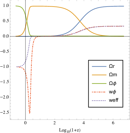
Refer to caption — Figure 1: The evolution of the density parameters and the equation of state parameters where we set $x_{1}-0.002=1\times 10^{-6}$ , $x_{2}=-1\times 10^{-13}$ , $x_{3}+0.008=1\times 10^{-6}$ , and $x_{4}=0.989$ at $\log_{10}(1+z)=6.73$ .

The Fig. 1 reveals that the evolution of the cuscuta-galileon with the exponential potential corresponds to the thermal history of the Universe correctly. This result is consistent with the stability analysis on the fixed points. The $w_{\phi}=1/3$ in the radiation dominated era, and then it is around zero in the matter dominated era. However, before approaching the de Sitter fixed point, the $w_{\phi}$ crosses the cosmological constant boundary, $w_{\Lambda}=-1$ , and then approaching $-1$ at late time. The large negative value can be understood by considering the evolution plot of the dynamical parameters as Fig. 2.

According to the Fig. 2, the $x_{1}$ and the $x_{4}$ tend to zero around the end of the matter dominated epoch, then the Eq. (20) becomes $w_{\phi}\simeq-w_{\rm eff}/x_{3}$ . Since $|x_{3}|<1$ , we find $|w_{\phi}|>|w_{\rm eff}|$ , and at late time the $|x_{3}|\rightarrow 1$ , thus $|w_{\phi}|\simeq|w_{\rm eff}|$ . Therefore, we obtain a large negative value of the $w_{\phi}$ around the end of the matter dominated era, and then it approaches to the $w_{\rm eff}$ at late time.

Note that the fine-tuning parameters are the amount of the radiation component, $x_{4}$ , and the ratio of velocity of the scalar field and the Hubble parameter squared, $x_{2}$ , in the radiation dominant to have long enough the matter dominant epoch. If $x_{4}$ is larger or $x_{2}$ is more negative, the matter dominant era will be shorter. It is then inconsistent with observations that the age of matter-radiation equality is around $z\approx 3300$ . The other parameters are more flexible, for example, $x_{1}$ and $x_{3}$ can be around $10^{-5}$ from the fixed point (c), we still obtain the sequence of the cosmic evolution properly. However, there is a small oscillations on the value of $w_{\phi}$ in this case.

V.2 Ghosts and Laplacian instability

As shown in §. IV, this model includes an additional degrees of freedom (a scalar field) in the present model. Then we have to check whether there exists no ghost or Laplacian instability in our cosmic evolution. Since there are three degrees of freedom, we expect that there exist scalar perturbations as well as tensor perturbations.

According to Refs. DeFelice:2011bh; Gergely:2014rna; Tsujikawa:2014mba; Kase:2014yya; Kase:2014cwa; Gleyzes:2013ooa the second order action of the tensor perturbations is

\displaystyle S_{2}^{T}=\int d^{4}x\frac{a^{3}}{4}L_{S}\Big[\dot{\gamma}_{ij}^{2}-c_{T}^{2}\frac{(\partial_{k}\gamma_{ij})^{2}}{a^{2}}\Big]\,,

(47)

where $\gamma_{ij}$ is the tensor perturbations which satisfies transverse and traceless conditions, $L_{S}$ relates to the action in the background level, and $c_{T}^{2}$ is a sound speed squared in the tensor mode which also relates to the action in the background level. In order to avoid ghosts the coefficient in front of the term $\dot{\gamma}_{ij}^{2}$ must be positive, thus we need the $L_{S}>0$ . Similarly, we require the $c_{T}^{2}>0$ to avoid the Laplacian instability.

For simplicity we use notations as the Ref. DeFelice:2011bh where they correspond to the action of the cuscuta-galileon (1) as follows

$\displaystyle{\cal W}_{1}$	$\displaystyle=$	$\displaystyle M_{\mathrm{PL}}^{2}\,,$	(48)
$\displaystyle{\cal W}_{2}$	$\displaystyle=$	$\displaystyle 2M_{\mathrm{PL}}^{2}H+2\dot{\phi}a_{3}=(2+x_{3})M_{\mathrm{PL}}^{2}H\,,$	(49)
$\displaystyle{\cal W}_{3}$	$\displaystyle=$	$\displaystyle-9M_{\mathrm{PL}}^{2}H^{2}-18H\dot{\phi}a_{3}$	(50)
	$\displaystyle=$	$\displaystyle(-9-9x_{3})M_{\mathrm{PL}}^{2}H^{2}\,,$	(50)
$\displaystyle{\cal W}_{4}$	$\displaystyle=$	$\displaystyle M_{\mathrm{PL}}^{2}\,,$	(51)

where $L_{S}\equiv{\cal W}_{1}/2$ and $c_{T}^{2}\equiv{\cal W}_{4}/{\cal W}_{1}$ . We then find

\displaystyle L_{S}=\frac{1}{2}M_{\mathrm{PL}}^{2}>0\,,~~~c_{T}^{2}=1\,.

(52)

Consequently, the cuscuta-galileon gravity satisfies the no ghosts and no Laplacian instability conditions of the tensor mode.

For the scalar perturbations it is similar to the tensor perturbations. In order to avoid the ghosts we require

\displaystyle Q_{S}\equiv\frac{{\cal W}_{1}(4{\cal W}_{1}{\cal W}_{3}+9{\cal W}_{2}^{2})}{3{\cal W}_{2}^{2}}=\frac{3x_{3}^{2}}{(2+x_{3})^{2}}>0\,,

(53)

and the sound speed squared in the scalar mode must be greater than zero to avoid the Laplacian instability:

\displaystyle c_{S}^{2}

\displaystyle\equiv

\displaystyle\frac{3\Big(-2{\cal W}_{1}^{2}\dot{\cal W}_{2}+2{\cal W}_{1}^{2}{\cal W}_{2}H-{\cal W}_{2}^{2}{\cal W}_{4}-2{\cal W}_{1}^{2}\Big((1+w_{m})\rho_{m}+(1+w_{r})\rho_{r}\Big)\Big)}{{\cal W}_{1}(4{\cal W}_{1}{\cal W}_{3}+9{\cal W}_{2}^{2})}=\frac{2x_{2}-x_{3}(8+x_{3})}{3x_{3}^{2}}>0\,.

(54)

Other conditions involving the existence of nonrelativistic matter and radiation fluids are automatically satisfied when we choose forms of the k-essence type perfect fluid as the Ref. Kase:2014yya.

The Fig. 3 reveals that the cuscuta-galileon gravity has no ghosts and the Laplacian instability in the scalar mode. In matter dominant and radiation dominant the sound speed squared is greater than unity because $|x_{3}|\ll 1$ in the denominator of the Eq. (54), while $x_{2}$ is about zero.

The results of the scalar perturbations reveal that there is a scalar degree of freedom propagating in this model, which is consistent with the analysis in the previous section.

We can construct a viable cosmological model in the cuscuta-galileon gravity theory. We show the cosmological evolution from radiation dominated era to de Sitter expansion stage via matter dominated era.

V.3 Observational constraints

However if we look into the detail, we find that the cuscuta-galileon gravity may not satisfy observations by several reasons. First, the Planck $2018$ results Aghanim:2018eyx reveal that the dark energy equation of state parameter is $w_{\rm DE}=-1.028\pm 0.031$ , it is consistent with the cosmological constant, while the cuscuta-galileon gives $w_{\phi}=-1.196$ at $\Omega_{m}=0.315$ . Second, there is a large amount of the dark energy component comparing to the cosmological constant in the matter and radiation dominated eras as Fig. 4.

From the Lambda-Cold Dark Matter ( $\Lambda$ CDM) model, the density parameter of the cosmological constant is given by

\displaystyle\Omega_{\Lambda}(z)=\frac{\Omega_{\Lambda}^{(0)}}{\Omega_{m}^{(0)}(1+z)^{3}+\Omega_{r}^{(0)}(1+z)^{4}+\Omega_{\Lambda}^{(0)}}\,,

(55)

where $\Omega_{m}^{(0)}=0.315$ , $\Omega_{r}^{(0)}=9\times 10^{-5}$ , and $\Omega_{\Lambda}=0.685$ according to the Planck $2018$ results. In the Fig. 4 we find that the $\Omega_{\phi}\sim\mathcal{O}(10^{-2})$ in the matter and radiation dominated epochs, whereas $\Omega_{\Lambda}$ is utterly small, for instance, at the last scattering surface, $z\approx 1090$ , the $\Omega_{\Lambda}\sim\mathcal{O}(10^{-9})$ . It is obvious that the model is different from the $\Lambda$ CDM model. Therefore, the cuscuta-galileon gravity is likely not to satisfy the observations which prefer the $\Lambda$ CDM model, such as the Cosmic Microwave Background (CMB) observations. Although rigorous calculations and global fitting with observational data are required, they are beyond the scope of this paper. Lastly, if we increase the $\lambda$ in order to obtain the lower $\Omega_{\phi}$ , such as $\lambda=10^{4}$ , we find $\Omega_{\phi}\sim\mathcal{O}(10^{-3})$ , the equation of state parameter of the scalar field will be more negative and more deviate from the observational value because $|x_{3}|\sim\mathcal{O}(10^{-3})\ll 1$ around the end of the matter dominated epoch.

VI Conclusions

In this work we study cosmological dynamics of the cuscuta-galileon gravity. The model was proposed in the Ref. deRham:2016ged as galileon generalization of the cuscuton model which is free from the caustic singularities in flat space-time. In the case without a potential term the equation of motion of the cuscuta-galileon does not depend on a scalar field, finding that there exists only the de Sitter expansion under the flat FLRW background. Thus in order to obtain the radiation and matter dominated eras we need to add a potential term, for which we consider two cases: an exponential potential and an inverse power-law potential. Using the dynamical system approach and studying stability of fixed points of the autonomous system, we find that only the exponential potential case can provide a proper sequence of the thermal history of the Universe successfully.

Even though there is no second-order time derivatives in the equation of motion, the results of the scalar perturbation reveal that there is a scalar degree of freedom propagating in this model. This is confirmed by using the Hamiltonian analysis where we find that the cuscuta-galileon gravity actually has three degrees of freedom and belongs to a subclass of Horndeski theories. In order to discuss the similar cuscuta-galileon theory with only two d.o.f., we have to include an additional kinetic term, which was discussed in Maeda:2022ozc.

In the perturbation level, the conditions for avoidance of ghosts and the Laplacian instability in the tensor mode are automatically satisfied by the form of the action. In the scalar mode we find that there is no ghost and Laplacian instabilities in the present cosmological model.

However, the detail numerical analysis reveals that there appears a large amount of the dark energy component in the matter and radiation dominated eras comparing to that in the $\Lambda$ CDM model. Therefore, the present cuscuta-galileon gravity may not satisfy the observational constraints.

Acknowledgements

S.P. would like to thank Aya Iyonaga and Shinji Tsujikawa for useful discussions. This work was supported in part by a Waseda University Grant for Special Research Project (No. 2020C-774) and by JSPS KAKENHI Grant Numbers JP17H06359 and JP19K03857.

Appendix A Cuscuta-galileon gravity without a potential term

Considering the action of the cuscuta-galileon gravity as Ref. deRham:2016ged in curved space-time up to cubic order:

	$\displaystyle S$	$\displaystyle=$	$\displaystyle\int d^{4}x\sqrt{-g}\Big[\frac{1}{2}M_{\mathrm{PL}}^{2}R+a_{2}\sqrt{-X}+a_{3}\ln\Big(-\frac{X}{\Lambda^{4}}\Big)\square\phi\Big]$		(56)
			$\displaystyle+S_{M}(g_{\mu\nu},\psi_{M})\,,$		(56)

Substituting the flat FLRW metric, $ds^{2}=-N(t)^{2}dt^{2}+a(t)^{2}\delta_{ij}dx^{i}dx^{j}$ , into the above action, and choosing the unitary gauge, $\phi=\phi(t)$ . Varying the action with respect to $\phi$ , after setting $N=1$ the equation of motion of the scalar field is given by

\displaystyle 6a_{3}H^{2}+2a_{3}\dot{H}-a_{2}H{\rm sgn}(\dot{\phi})=0\,.

(57)

Since the above equation depends on $H$ only, we can integrate it directly. The evolution of the Hubble parameter is

\displaystyle H(t)=\frac{a_{2}{\rm sgn}(\dot{\phi})}{6a_{3}-e^{-(a_{2}{\rm sgn}(\dot{\phi})(t+C)/2a_{3})}}\,,

(58)

where $C$ is a constant of integration. If $a_{2}{\rm sgn}(\dot{\phi})/2a_{3}>0$ , we find

\displaystyle\lim_{t\rightarrow\infty}H(t)=\frac{a_{2}{\rm sgn}(\dot{\phi})}{6a_{3}}={\rm constant}\,.

(59)

Then, we obtain the de Sitter solution at late time. If $a_{2}{\rm sgn}(\dot{\phi})/2a_{3}<0$ , we find

\displaystyle\lim_{t\rightarrow\infty}H(t)=0\,.

(60)

This is the static universe solution; however, this solution is contradict with observations. We thus accept only the de Sitter solution.

Using the dynamical system approach as the section III, if the cuscuta-galileon model does not have a potential term, then the $x_{1}=0$ and the $\lambda$ is undefined. Therefore we have only $3$ autonomous equations (15) - (17) with $3$ parameters. Setting $dx_{2}/dN=dx_{3}/dN=dx_{4}/dN=0$ , we find fixed points as Table 3.

Fixed point	$x_{2}$	$x_{3}$	$x_{4}$	$\Omega_{m}$	$\Omega_{r}$	$\Omega_{\phi}$	$w_{\phi}$	$w_{\rm eff}$
(i)	$-3$	$-1$	$0$	$0$	$0$	$1$	$-1$	$-1$
(j)	$0$	$-1$	$0$	$0$	$0$	$1$	$1$	$1$

Table 3: The fixed points, the density parameters, and the equation of state parameters of the cuscuta-galileon without a potential.

The fixed point (i) can be the dark energy dominated epoch, whereas the point (j) does not match with any thermal history of the Universe. Then we obtain only the de Sitter expansion in the cuscuta-galileon gravity without a potential term. This result is consistent with the analytic solution (59).

Appendix B Two independent equations

There are three basic equations, but they are not independent. For example, taking the time derivative of Eq.(3) and eliminating $\ddot{\phi}$ by use of Eq. (4) and the equations of $\dot{\rho}_{i}$ ( $i=m,r$ ), i.e.,

\dot{\rho}_{i}+3H(\rho_{i}+P_{i})=0\,,

we obtain Eq. (5).

In fact we obtain the following two independent equations:

	$\displaystyle\ddot{\phi}-{3a_{3}\over M_{PL}^{2}}\dot{\phi}^{2}+\left(3\dot{\phi}+{a_{2}\over 2a_{3}^{2}}M_{PL}^{2}{\rm sgn}(\dot{\phi})\right)\sqrt{\left({a_{3}\over M_{PL}^{2}}\dot{\phi}\right)^{2}+{1\over 3M_{PL}^{2}}\left(\rho_{m}+\rho_{r}+V\right)}$
	$\displaystyle~~~-{1\over 2a_{3}}\left(\rho_{m}-P_{m}+\rho_{r}-P_{r}+2V\right)+{M_{PL}^{2}\over 6a_{3}^{2}}V_{,\phi}=0\,,$		(61)
	$\displaystyle H\equiv{\dot{a}\over a}=-{a_{3}\over M_{PL}^{2}}\dot{\phi}+\sqrt{\left({a_{3}\over M_{PL}^{2}}\dot{\phi}\right)^{2}+{1\over 3M_{PL}^{2}}\left(\rho_{m}+\rho_{r}+V\right)}\,.$
			(62)

Eq. (61) is the second order differential equation for $\phi$ , while Eq. (62) is the first differential equation for $a$ . $P_{m}\,,\rho_{m}$ and $P_{r}\,,\rho_{r}$ are given by a scale factor $a$ as

\displaystyle P_{m}=0\,,~\rho_{m}\propto a^{-3}\,,

(63)

and

\displaystyle P_{r}={\rho_{r}\over 3}\,,~\rho_{r}\propto a^{-4}\,.

(64)

Hence once we know the initial values of $\phi\,,\dot{\phi}\,,\rho_{m}\,,\rho_{r}$ and $a$ , we find the time evolution of those variables.

References

(1) A. G. Riess et al. [Supernova Search Team], Astron. J. 116 (1998), 1009-1038 doi:10.1086/300499 [arXiv:astro-ph/9805201 [astro-ph]].
(2) S. Perlmutter et al. [Supernova Cosmology Project], Astrophys. J. 517 (1999), 565-586 doi:10.1086/307221 [arXiv:astro-ph/9812133 [astro-ph]].
(3) G. W. Horndeski, Int. J. Theor. Phys. 10 (1974), 363-384 doi:10.1007/BF01807638
(4) C. Deffayet, X. Gao, D. A. Steer and G. Zahariade, Phys. Rev. D 84 (2011), 064039 doi:10.1103/PhysRevD.84.064039 [arXiv:1103.3260 [hep-th]].
(5) T. Kobayashi, M. Yamaguchi and J. Yokoyama, Prog. Theor. Phys. 126 (2011), 511-529 doi:10.1143/PTP.126.511 [arXiv:1105.5723 [hep-th]].
(6) L. Heisenberg, JCAP 05 (2014), 015 doi:10.1088/1475-7516/2014/05/015 [arXiv:1402.7026 [hep-th]].
(7) C. de Rham and G. Gabadadze, Phys. Rev. D 82 (2010), 044020 doi:10.1103/PhysRevD.82.044020 [arXiv:1007.0443 [hep-th]].
(8) C. de Rham, G. Gabadadze and A. J. Tolley, Phys. Rev. Lett. 106 (2011), 231101 doi:10.1103/PhysRevLett.106.231101 [arXiv:1011.1232 [hep-th]].
(9) C. M. Will, Living Rev. Rel. 17 (2014), 4 doi:10.12942/lrr-2014-4 [arXiv:1403.7377 [gr-qc]].
(10) J. Khoury and A. Weltman, Phys. Rev. Lett. 93 (2004), 171104 doi:10.1103/PhysRevLett.93.171104 [arXiv:astro-ph/0309300 [astro-ph]].
(11) J. Khoury and A. Weltman, Phys. Rev. D 69 (2004), 044026 doi:10.1103/PhysRevD.69.044026 [arXiv:astro-ph/0309411 [astro-ph]].
(12) K. Hinterbichler and J. Khoury, Phys. Rev. Lett. 104 (2010), 231301 doi:10.1103/PhysRevLett.104.231301 [arXiv:1001.4525 [hep-th]].
(13) P. Brax, C. van de Bruck, A. C. Davis and D. Shaw, Phys. Rev. D 82 (2010), 063519 doi:10.1103/PhysRevD.82.063519 [arXiv:1005.3735 [astro-ph.CO]].
(14) C. Burrage and J. Khoury, Phys. Rev. D 90 (2014) no.2, 024001 doi:10.1103/PhysRevD.90.024001 [arXiv:1403.6120 [hep-th]].
(15) S. Panpanich, S. Ponglertsakul and K. Maeda, Phys. Rev. D 100 (2019) no.4, 044038 doi:10.1103/PhysRevD.100.044038 [arXiv:1902.00265 [gr-qc]].
(16) P. Brax, C. Burrage and A. C. Davis, JCAP 01 (2013), 020 doi:10.1088/1475-7516/2013/01/020 [arXiv:1209.1293 [hep-th]].
(17) E. Babichev, C. Deffayet and R. Ziour, Int. J. Mod. Phys. D 18 (2009), 2147-2154 doi:10.1142/S0218271809016107 [arXiv:0905.2943 [hep-th]].
(18) E. Babichev and C. Deffayet, Class. Quant. Grav. 30 (2013), 184001 doi:10.1088/0264-9381/30/18/184001 [arXiv:1304.7240 [gr-qc]].
(19) A. I. Vainshtein, Phys. Lett. B 39 (1972), 393-394 doi:10.1016/0370-2693(72)90147-5
(20) A. Nicolis, R. Rattazzi and E. Trincherini, Phys. Rev. D 79 (2009), 064036 doi:10.1103/PhysRevD.79.064036 [arXiv:0811.2197 [hep-th]].
(21) N. Afshordi, D. J. H. Chung and G. Geshnizjani, Phys. Rev. D 75 (2007), 083513 doi:10.1103/PhysRevD.75.083513 [arXiv:hep-th/0609150 [hep-th]].
(22) N. Afshordi, D. J. H. Chung, M. Doran and G. Geshnizjani, Phys. Rev. D 75 (2007), 123509 doi:10.1103/PhysRevD.75.123509 [arXiv:astro-ph/0702002 [astro-ph]].
(23) N. Afshordi, Phys. Rev. D 80, 081502 (2009) doi:10.1103/PhysRevD.80.081502 [arXiv:0907.5201 [hep-th]].
(24) C. Lin and S. Mukohyama, JCAP 10 (2017), 033 doi:10.1088/1475-7516/2017/10/033 [arXiv:1708.03757 [gr-qc]].
(25) K. Aoki, C. Lin and S. Mukohyama, Phys. Rev. D 98 (2018) no.4, 044022 doi:10.1103/PhysRevD.98.044022 [arXiv:1804.03902 [gr-qc]].
(26) K. Aoki, A. De Felice, C. Lin, S. Mukohyama and M. Oliosi, JCAP 01 (2019), 017 doi:10.1088/1475-7516/2019/01/017 [arXiv:1810.01047 [gr-qc]].
(27) S. Mukohyama and K. Noui, JCAP 07 (2019), 049 doi:10.1088/1475-7516/2019/07/049 [arXiv:1905.02000 [gr-qc]].
(28) A. De Felice, A. Doll and S. Mukohyama, JCAP 09 (2020), 034 doi:10.1088/1475-7516/2020/09/034 [arXiv:2004.12549 [gr-qc]].
(29) K. Aoki, A. De Felice, S. Mukohyama, K. Noui, M. Oliosi and M. C. Pookkillath, Eur. Phys. J. C 80, no.8, 708 (2020) doi:10.1140/epjc/s10052-020-8291-1 [arXiv:2005.13972 [astro-ph.CO]].
(30) A. Iyonaga, K. Takahashi and T. Kobayashi, JCAP 12 (2018), 002 doi:10.1088/1475-7516/2018/12/002 [arXiv:1809.10935 [gr-qc]].
(31) A. Iyonaga, K. Takahashi and T. Kobayashi, JCAP 07 (2020), 004 doi:10.1088/1475-7516/2020/07/004 [arXiv:2003.01934 [gr-qc]].
(32) J. Gleyzes, D. Langlois, F. Piazza and F. Vernizzi, Phys. Rev. Lett. 114 (2015) no.21, 211101 doi:10.1103/PhysRevLett.114.211101 [arXiv:1404.6495 [hep-th]].
(33) C. de Rham and H. Motohashi, Phys. Rev. D 95 (2017) no.6, 064008 doi:10.1103/PhysRevD.95.064008 [arXiv:1611.05038 [hep-th]].
(34) T. Baker, E. Bellini, P. G. Ferreira, M. Lagos, J. Noller and I. Sawicki, Phys. Rev. Lett. 119 (2017) no.25, 251301 doi:10.1103/PhysRevLett.119.251301 [arXiv:1710.06394 [astro-ph.CO]].
(35) P. Creminelli and F. Vernizzi, Phys. Rev. Lett. 119 (2017) no.25, 251302 doi:10.1103/PhysRevLett.119.251302 [arXiv:1710.05877 [astro-ph.CO]].
(36) J. Sakstein and B. Jain, Phys. Rev. Lett. 119 (2017) no.25, 251303 doi:10.1103/PhysRevLett.119.251303 [arXiv:1710.05893 [astro-ph.CO]].
(37) J. M. Ezquiaga and M. Zumalacárregui, Phys. Rev. Lett. 119 (2017) no.25, 251304 doi:10.1103/PhysRevLett.119.251304 [arXiv:1710.05901 [astro-ph.CO]].
(38) R. Bean, S. H. Hansen and A. Melchiorri, Phys. Rev. D 64 (2001), 103508 doi:10.1103/PhysRevD.64.103508 [arXiv:astro-ph/0104162 [astro-ph]].
(39) S. Tsujikawa, Lect. Notes Phys. 892 (2015), 97-136 doi:10.1007/978-3-319-10070-8_4 [arXiv:1404.2684 [gr-qc]].
(40) R. Kase and S. Tsujikawa, Phys. Rev. D 90 (2014), 044073 doi:10.1103/PhysRevD.90.044073 [arXiv:1407.0794 [hep-th]].
(41) R. Kase and S. Tsujikawa, Int. J. Mod. Phys. D 23 (2015) no.13, 1443008 doi:10.1142/S0218271814430081 [arXiv:1409.1984 [hep-th]].
(42) C. Lin, S. Mukohyama, R. Namba and R. Saitou, JCAP 10 (2014), 071 doi:10.1088/1475-7516/2014/10/071 [arXiv:1408.0670 [hep-th]].
(43) A. De Felice and S. Tsujikawa, JCAP 02 (2012), 007 doi:10.1088/1475-7516/2012/02/007 [arXiv:1110.3878 [gr-qc]].
(44) L. Á. Gergely and S. Tsujikawa, Phys. Rev. D 89 (2014) no.6, 064059 doi:10.1103/PhysRevD.89.064059 [arXiv:1402.0553 [hep-th]].
(45) J. Gleyzes, D. Langlois, F. Piazza and F. Vernizzi, JCAP 08 (2013), 025 doi:10.1088/1475-7516/2013/08/025 [arXiv:1304.4840 [hep-th]].
(46) N. Aghanim et al. [Planck], Astron. Astrophys. 641 (2020), A6 doi:10.1051/0004-6361/201833910 [arXiv:1807.06209 [astro-ph.CO]].
(47) K. Maeda and S. Panpanich, Phys. Rev. D 105 (2022) no.10, 104022 doi:10.1103/PhysRevD.105.104022 [arXiv:2202.04908 [gr-qc]].