Towards A Measure of General Machine Intelligence
Abstract
To build general-purpose artificial intelligence systems that can deal with unknown variables across unknown domains, we need benchmarks that measure how well these systems perform on tasks they have never seen before. A prerequisite for this is a measure of a task’s generalization difficulty, or how dissimilar it is from the system’s prior knowledge and experience. If the skill of an intelligence system in a particular domain is defined as it’s ability to consistently generate a set of instructions (or programs) to solve tasks in that domain, current benchmarks do not quantitatively measure the efficiency of acquiring new skills, making it possible to brute-force skill acquisition by training with unlimited amounts of data and compute power. With this in mind, we first propose a common language of instruction, a programming language that allows the expression of programs in the form of directed acyclic graphs across a wide variety of real-world domains and computing platforms. Using programs generated in this language, we demonstrate a match-based method to both score performance and calculate the generalization difficulty of any given set of tasks. We use these to define a numeric benchmark called the generalization index, or the g-index , to measure and compare the skill-acquisition efficiency of any intelligence system on a set of real-world tasks. Finally, we evaluate the suitability of some well-known models as general intelligence systems by calculating their g-index scores.
Contents
1 Introduction
1.1 History of defining intelligence
The concept of intelligence has been expressed in informal terms from time immemorial, but to date there has been no consensus on a formal definition [18]. In psychology, definitions of intelligence include “the faculty of adapting one’s self to circumstances” [3], and “the aggregate or global capacity . .. to act purposefully, to think rationally, and to deal effectively with [the] environment”, [1]. The definition of artificial intelligence observes similar variety, with common reliance on a human reference; for eg. “machines capable of performing tasks that would require intelligence if done by humans” [4, 16]. Developments in the field of AI have led to further refinements, with terms such as skill-based, narrow, or weak AI versus general or strong AI [28, 13, 31].
The Turing test “imitation game” [2], one of the first measures of artificial intelligence was qualitative in nature. It required that an artificial intelligence convince a human judge that it was a human. This created an inaccurate perception of an AI’s capabilities due to variance in the judge’s knowledge [19]. The improvements to the Turing test (such as the Lovelace test [23] and its successor [36]) maintain the requirement of a human or human-like judge, focusing on the judge’s available resources and formal descriptions of what the judge can use for measuring the AI’s capabilities. Till date, subjective human judgment plays a key role in evaluating any intelligence system.
1.2 Intelligence as benchmarks of skill
Recent breakthroughs in the capabilities of machine intelligence systems have relied upon the scaling of computational methods such as support vector machines, random forests and neural networks. While this was assisted by the increased availability of raw computing power, we note that framing machine intelligence in terms of computation enabled quantitative methods for evaluation, as measuring the performance of a system was simplified to computing a numerical benchmark score on a publicly available dataset. The MNIST dataset [20] served as a benchmark for digit classification [24, 27, 25] , and is used today in introductory texts to showcase the power of deep neural networks. Over the years, designing a good benchmark has developed into a specialized problem, involving the collection of large diverse datasets spanning multiple years [52].

The presence of quantitative benchmarks was a boon for developing machine learning-based intelligence systems, as one could compare different methods and design targeted improvements to build upon a consistent, computable, numerical score. The state-of-the-art in image classification improved every year since the ImageNet benchmark [30] became widely available, starting with AlexNet in 2012 [35], to SENet [49] in 2017 (see Figure 1), with new techniques such as ResNet skip-connections gaining prominence on the back of their ImageNet performance. Similar improvements were also seen in the field of language understanding, with the GLUE benchmark [47] and the development of well-known transformer models like BERT [44] and GPT-2 [51].
1.3 Measuring general intelligence
Deep learning-based methods have achieved a high level of skill in specialized tasks, but it is still hard to quantitatively measure the “generalization capability” of an intelligence system - or its “ability to handle situations (or tasks) that differ from previously encountered situations” [48]. This is due to the difficulty of measuring the variables involved in current definitions of artificial intelligence. [26] informally define intelligence as measuring an “agent’s ability to achieve goals in a wide range of environments”. It further mentions the properties desirable in a measure of intelligence, such as a formal mathematical definition, applicability across different methods without bias, and an informative, numerical score to enable comparison across agents. However, an agent’s intelligence cannot be computed practically according to this definition as it relies on finding the Kolmogorov complexity [29] of each environment .
[40] bifurcates the measurement of intelligence systems into task-oriented and ability-oriented evaluations. Both are important for evaluating a system, but the former is far more common. Task-oriented evaluations include human judgments of AI performance, direct benchmark comparisons, and assessment of adversarial situations in games such as playing Chess or Go. Ability-oriented evaluations take the form of psychometrics in the case of human intelligence, and extend to artificial systems [34] when intelligence is viewed as a form of information processing [17]. This allows the use of algorithmic information theory (AIT) [15] to perform ability-oriented evaluations of artificial systems. Building on this, [48] provides an outline for the measurement of intelligence via a framework that is easily mapped to current methods in machine learning. The intelligence of a system here is defined as “the measure of its skill-acquisition efficiency over a scope of tasks, with respect to priors, experience, and generalization difficulty”, and involves testing via a benchmark dataset called the Abstract Reasoning Corpus (ARC). However, this framework does not offer a quantitative measure of generalization difficulty, and all evaluation is close-ended and binary.
In this paper, we define the generalization index, abbreviated to g-index, a quantitative benchmark to measure the intelligence of an artificial system as a computable, numerical value. The naming is inspired from the g-factor, which is a measure of general ability in the field of psychometrics [21]. It accounts for performance, generalization difficulty and sample efficiency across a wide range of real-world tasks. Section 2 describes the experimental setup for the benchmark, and showcases the components that enable calculating numerical values for evaluation. Section 3 formally defines the parameters on which the g-index depends, constructs a mathematical formula, and shows how the properties of the g-index follow the guidelines in current literature. Section 4 evaluates some well-known transformer models as candidates for a general intelligence system by computing their g-index scores, and provides a sample dataset of real-world tasks and their associated skill programs that can be used with the g-index 11 1 https://github.com/mayahq/g-index-benchmark. Section 5 adapts the g-index for a toy environment with a simpler program space. Finally, Section 6 notes possible directions for improvement in the current design and of the g-index .
2 Setting up the evaluation
2.1 Components of the g-index
In this section, we describe the details of the components required to compute the g-index benchmark. We follow the terminology from [48], as it is easily mapped to supervised learning and reinforcement learning. The description of the evaluation setup can be given as follows:
- •
A task is specified to an intelligence system .
- •
The intelligence system generates a skill program to solve the task. The intelligence system has been trained on a training set (or a curriculum ) of tasks that may or may not be related to .
- •
A scoring function evaluates the responses of the skill program against possible situations of the task, and provides a score along with some feedback if available.
- •
The intelligence system can be updated based on the evaluation and feedback of the scoring function.
- •
The generalization difficulty of a task measures how different is from the curriculum of the intelligence system. It can be used to weight the system’s performance for varying degrees of unseen task specifications.
While previous definitions of general intelligence rely on quantities like Kolmogorov complexity [29] which are difficult to compute, the components in our setup together enable computing numerical values that can be combined to measure the capabilities of an intelligence system. The skill program is expressed in a custom programming language that can be extended to construct new programs without additional syntax complexity, which streamlines collecting and augmenting data for the intelligence system. The scoring function does not require running the program to compute the score, which means it can also be used as a loss function or reward function for training the intelligence system. Finally, we construct an intuitive formulation of generalization difficulty based on nearest neighbors that reuses the scoring function. These features are described in the subsections that follow.
2.2 The Task Specification
Human beings follow a sequence of steps to perform a specified task. For an artificial intelligence system, the equivalent sequence of steps is the program. Hence to perform a task, the system would need to generate (or synthesize) programs, when provided a specification via examples of inputs, in natural language, images, audio, or video.
The field of program synthesis deals with the automatic construction of programs that are consistent with a given task specification [5]. The common form of a task specification is a set of input-output examples [6, 11] from which the necessary program(s) can be synthesized. The application of deep learning to program synthesis is called neural program synthesis . Many neural program synthesis techniques have the task specified via a set of input-output examples [38] , but some also use natural language text prompts [41], demonstration videos [46], or combinations of these as well[58, 68].
In our current setup, the tasks submitted to the intelligence system are specified in English without listing any input-output examples. When scoring the generated program, an associated reference program is provided.
2.3 The Skill Program
The choice of target programming language for synthesis varies across implementations. [42] describe the generation of Python code snippets from a given description. [41] use recurrent neural networks (RNNs) to produce shell scripts. Codex [63], which uses a large language model similar to GPT-3 [53], generates entire functions in Python from documentation strings, with similar capabilities being extended to other common programming languages. It is also common to use a domain-specific language (DSL). DSLs for program synthesis may be designed from scratch for a specific purpose [37], a restricted subset of a language [58, 43] or an extended version of an existing language [66].
2.3.1 Programs as directed acyclic graphs
In our current setup, the intelligence system synthesizes programs that follow the flow-based programming (FBP) paradigm [7, 32]. Flow-based programs are networks of nodes, each encapsulating a ”black box” process, transferring data across predefined connections. Flow-based programs are expressed as directed acyclic graphs (DAGs) consisting of nodes with various attributes, that are designed to be reusable and wired together to perform any task. The exact syntax of flow-based programs can vary, but can usually be converted into an order-independent array in Javascript Object Notation (JSON [33, 39]), a data interchange format derived from Javascript. Node-RED [67] and NoFloJS [61] are popular Javascript packages that enable writing flow-based programs, and both allow for the programs to be saved as JSON. There are several advantages to have the intelligence system synthesizing programs in the flow-based paradigm:
- •
Human-friendly and machine-friendly skill programs: Flow-based program JSONs can be displayed in a visual programming interface where one can see all the nodes, their connections, global program configuration and possible errors. This makes it easy for humans to construct, edit, and interpret flow programs. The key-value syntax of JSON imposes constraints that make it less complicated than full languages like Javascript and Python, which helps when synthesizing the program DAG. Figure 2 provides an example of a flow program along with the JSON specification of selected nodes.

Figure 2: Representing a flow-based program as a DAG: The JSON descriptions of three nodes are displayed - each node instance has unique id for reference and wires connecting it to other nodes. For the maya-browser-query type node, the attributes include mergeOutputs and options. The csv type node has a wire connecting it to the file node via its unique id. - •
Extensible via custom nodes: Every node in a flow-based program is assigned a special type attribute, and all nodes with the same type contain the same attribute keys. Most FBP implementations provide a default library of node types for constructing programs, but we can also create and add new node types that encapsulate a custom functionality for our own use22 2 For examples of reusable nodes see the library in Appendix B.. This allows for maximum extensibility and reusability within the same level of expressivity: adding a new node type increases the number of possible skill programs without changing the language syntax or bloating program size.
- •
Perform variety of tasks: Each node JSON description in the FBP is an abstraction linked to a particular black box process. The functionality encapsulated in each node can be implemented in any programming language across platforms. This means that flow-based program can be deployed on desktop computers, on servers in the cloud, and even on embedded devices such as the Raspberry Pi and Arduino. This allows us to specify tasks that may be performed across multiple devices, locally or over the internet. Figure 3 shows four different tasks with their associated flow-based skill programs.

Figure 3: Program DAGs to : 1. Open browser tab, search for and play a video on Youtube. 2. Search for a given query in a browser using Google Search, scrape the results and save them to a file. 3. Show a dashboard for controlling an Industrial IOT setup and 4. Remotely control a drone using MQTT messages - •
Constrained program design: The design of flow-based programs can be restricted in three ways:
- 1.
The limited syntax of JSON and the DAG construction makes it difficult to use advanced programming constructs like recursion and loops.
- 2.
If necessary, the library of available nodes can be customized to prevent the intelligence system from using specific nodes.
- 3.
If certain node properties are confusing or risky (such as allowing arbitrary code execution), they can be restricted by designing new nodes that do not allow such modifications.
Proper restrictions along these axes can limit program aliasing – the existence of multiple valid programs that satisfy the task specification – by providing one obvious direction to solve a given task.
- 1.
- •
Efficient program generation - Program synthesis methods based on deep learning may have limits on the size of synthesized programs. For instance, neural network architectures like transformers have a fixed upper bound on the number of tokens that can be generated, so it is important to use the available token space efficiently. With flow-based programs, we can succinctly specify nodes that perform complex tasks due to the power of encapsulation. This allows for a larger space from which the intelligence system can generate programs.
- •
Evaluating a generated program: The programs synthesized by the intelligence system are evaluated by the scoring function. It is impractical to evaluate the outputs of the skill program against all possible inputs, so approximate techniques are used, such as comparing program structure or using special input cases. Programs written in Javascript or Python may be difficult to evaluate without testing due to program aliasing. Since program aliasing can be minimized for flow-based programs, they can be evaluated without having to run the program.
- •
Language-agnostic skill programs: The nodes used in flow-based programs encapsulate black-box processes, which means that the underlying implementations can be in any programming language. Flow-based programs hence simply act as a coordination layer between implementations of different pieces of logic. This means that models that learn how to synthesize these DAGs only need to learn the abstract relationship between task input and its solution program, leaving the low-level details free to be implemented in any manner. Figure 4 shows flow-based programs across different tasks.

Figure 4: Since flow-based programs are simply the coordination logic to compose any set of processes together, these process components can be built using any framework, language, application or API, leading to a wide range of applications.
2.3.2 DAGs vs Abstract Syntax Trees
While programs in other programming languages can be analysed as graphs by examining their Abstract Syntax Trees (AST) representations, the DAGs of flow-based programs are easier to compare with one another due to the following reasons:
- •
The order of nodes in the AST is dependent on the order of text in the program source. For our program DAGs, the order of the program is specified implicitly in the program source by the edges between nodes. DAG comparisons are less affected by the order of information specified in the program source compared to AST comparisons.
- •
AST representations suffer from program aliasing–two programs that satisfy the same task can have completely different ASTs. For our program DAGs, we can minimize program aliasing by constraining the kinds of nodes that are allowed for use.
- •
For complex specifications, the program size (and therefore AST size) can grow arbitrarily large if encapsulation is not used, which makes it harder to compare two given programs. Our program DAGs are designed to benefit from encapsulation: each node can encapsulate a “black-box” process of arbitrary complexity, and the attributes of the node are used to examine and control the behavior of the process.
- •
The AST is a low-level representation of the program: it is used to ensure that the program source is syntactically valid, check for minor semantic errors (like dereferencing null pointers) and perform program optimizations. It is difficult to reason about the behavior of the program from looking at its AST representation. The DAG is a high-level representation of the flow-based program: we can infer the program’s general behavior from the DAG structure and the node types, and examine node attributes to understand or change the behavior of any component.
2.4 The scoring function
After a skill program has been synthesized by the intelligence system, it is evaluated by a scoring function. The program can be evaluated by its success on a special set of input-output pairs, or by match-based metrics. For a given task, match-based metrics compute similarity by comparing the structure a generated program with a known reference program. This reference could be provided by a human, generated via a fixed set of rules, augmented from existing data, or synthesized by another intelligence system. The BLEU score [22] can be used to compare the text of the two given programs, but it does not consider the structured syntax or the semantic features of the programs. CodeBLEU [57] improves upon the BLEU score by comparing the abstract syntax trees (AST) and the semantic dataflow of the programs. While match-based metrics do not need to run the generated program for evaluation, they are affected by program aliasing. Recent synthesis methods [50, 56, 63] evaluate programs via functional correctness, wherein a generated program is considered correct if it passes a set of unit tests33 3 Unit tests include a set of known input-output pairs, but may also contain collections of inputs that together test for the presence of certain properties such as types of failures in a given program.. Functional correctness is useful because it is similar to how humans evaluate programs written by each other, but it requires running the generated program to obtain a score.
2.4.1 Divergence Metric for Flow-Based Programs
In Subsection 2.3 we noted that flow-based programs can be constrained to minimize the program aliasing, and the DAG representations are easier to compare than ASTs (Subsubsection 2.3.2). Hence for our scoring function, we use a match-based divergence metric to compare the DAG of the generated program with a known reference.
- •
Let be a known reference skill program, and be a skill program generated by the intelligence system.
- •
Let be the DAG denoting the . Here, and refer to the vertices and edges of respectively, and .
- •
Let be the DAG denoting the program . Here, and refer to the vertices and edges of respectively, and .
Given two programs , the divergence metric accepts their DAGs as input and is constrained as follows:
| (1) | ||||||||
2.4.2 Computing for a Single Node
Consider the simple case for , where the DAGs and both contain only one attributed node and zero edges. If is the only node in and the only node in , we can compare the attributes of with those in to obtain a node similarity value .
- •
If both nodes have different types,
- •
If both nodes have the same type, they will have the same attribute keys. Node attribute values follow a binary comparison. If is number of attributes for a given node type, and is the number of attribute values that are equal for both nodes, then
- •
If both nodes have the same type, and all node properties are equal, .
Thus when , both contain only one node and zero edges, we define as
| (2) |
We can see that the value of follows the constraints given in Equation 1 for the simple case.
2.4.3 Computing for the General Case
When computing the value of between two arbitrary DAGs, we would need to consider the common substructure between the DAGs in addition to the node-wise similarity values. The value of should be low when the DAGs have highly similar structure, so we compute it by finding the largest subgraph common to both DAGs. This is known as the maximum common edge subgraph problem (MCES) [14], an extension of the subgraph isomorphism problem [10]. Two graphs and are isomorphic to each oher () if there exists a bijection that preserves the graph structure:
| (3) |
We need to find subgraphs and that are isomorphic to each other, ie . This requires that and have the same number of vertices, ie
and a bijection between the subgraphs that satisfies Equation 3. and also need to be the largest common subgraphs
| (4) | ||||
We obtain , , and the bijective mapping by constructing an association graph between the nodes of and , and finding a maximum clique in [9, 12]. Appendix C explains the process of obtaining in detail, including the rules for construction of the association graph and ensuring the properties of from Equation 1 are satisfied. Figure 5 provides a visual overview of the process. Once we obtain , we calculate the value of the metric is using each node in , and its image via in . If , then
| (5) |

2.4.4 Features of
While has an exponential complexity due to the use of subgraph isomorphism, in practice, the computation of is sped up as Equation 11 reduces the number of vertices in the association graph , and Equation 12 tends to produces sparser graphs. As does not require the execution of the generated programs, it can be used in the training loop of supervised or reinforcement learning methods.
With the match-based DAG divergence metric , we now have a scoring function to compare a generated flow-based program with a reference program . Flow-based programs can be expressed in JSON, so a JSON parser can be used to ensure valid syntax. The DAGs constructed from the valid JSON can then be input to to compare the semantic dataflow of the programs. Since enables the comparison of any two flow-based programs, it can be extended to measure the dissimilarity of a program from a given set of programs, and more generally measure the dissimilarity between two sets of programs, by computing all necessary pairwise comparisons.
The values of are based on the structural differences between the DAGs and consider degrees of errors in the generated program:
- •
Syntax Errors: The generated program has incorrect JSON syntax, resulting in a reduced or incomplete DAG after parsing.
- •
Function Errors: Some nodes are incorrectly specified or missing from the generated DAG. If a node in the generated DAG has only one differing attribute compared to the reference, it is reflected in when computing the node similarity .
- •
Dataflow Errors: The generated program has the same nodes as the reference, but has different edges, denoting different semantics.
2.5 Measuring Generalization Difficulty
Humans have the capability to generalize, or they are able to use past learning experience to navigate new situations in the present. A machine intelligence would need to possess similar capabilities to deal with new or unseen task specifications. In machine learning, generalization deals with a model’s performance on previously unseen data samples that are similar to the distribution of the training set of the model. A model is said to have overfit the training data if predicts well on the training data, but fails to predict on new unseen samples. In deep learning, it is common to use some regularization techniques to avoid overfitting.
In the context of the g-index and our experimental setup, we focus on the generalization difficulty of a specified task. For a given task , [48] informally defines generalization difficulty as “a measure of how much the shortest training-time solution program needs to be edited in order to become an appropriate evaluation-time solution program”, and relies on Relative Algorithmic Complexity to compute the edit difference between the programs. We rephrase this statement for our experiment setup as follows: Suppose an intelligence system , trained on a curriculum of tasks , is given a task . If is an appropriate evaluation-time program that solves the task , how much does differ from the training-time solution programs for tasks ?
Since the skill programs generated by the intelligence system in our experimental setup are flow-based programs, they can be expressed as DAGs. Therefore, if is an optimal flow-based program that solves the task , we can use the metric defined in Subsection 2.4 and quantify the difference between and programs generated for tasks in the curriculum by a nearest neighbor search. Thus, we can define the domain distance of a single task for an intelligence system trained on a curriculum of tasks as :
| (6) | ||||
Note that is bounded between . If it means that the task can be found in the training set , and hence no generalization is required.

If is too large, the value can be approximated by clustering the elements of into task domains using the divergence metric : two tasks within the same domain are “closer” to each other () than tasks in different domains. Figure 6 shows an example of task domains and their related divergence scores.
The definition of in Equation 6 enables the computation of generalization difficulty within of the training-set/test-set paradigm that is commonly used for training machine learning models. By computing , a model’s performance on an unseen dataset can be weighted in context of the generalization difficulty of the tasks in the set.
3 The g-index benchmark
3.1 Defining the formula
We now define the formula for computing the g-index based on the experimental setup defined in Section 2. First, we describe the necessary variables:
- •
An intelligence system generates a flow-based skill program when input the specification for a given task . This formulation is method-agnostic, and allows the g-index benchmark to apply not only for deep-learning based systems of today, but also be extended to any new techniques in the future, by plugging in the variables measured below.
- •
The intelligence system is trained on a curriculum , consisting of tasks and their associated reference skill programs . We expect that the ideal intelligence system would also be the most sample-efficient in terms of training – it would learn to solve a large variety of tasks from just a single demonstration. Hence the value of g-index should decrease as the number of training samples increases.
- •
A curriculum domain , refers to a subset of where all tasks belong to the same task domain. We expect that an ideal intelligence system would be able to generalize from the least number of tasks provided per domain. So, the value of the g-index for the system should decrease as more tasks are provided for a given domain. We define , the weight of considering curriculum tasks from as:
- •
The priors of the system refer to knowledge built into the system before any training. Examples of priors include previously learnt weights, neural network architectures, data pre-processing techniques, program optimizations etc. We expect that the ideal intelligence system would be able to generalize from having the least amount of built-in priors. Hence the value of the g-index should decrease as more priors are encoded into the system. For our experiments, we consider the value of as a fixed constant, but we expect this to change as more complex systems are evaluated.
- •
When training the intelligence system on a curriculum , it is important to measure the experience of the system with . The units of measure for compute power are FLOPS(Floating Point Operations Per Second) or MIPS(Million Instructions Per Second), which are reflective of the rate at which the system is exposed to the data. We expect that the ideal intelligence system would be one that exhibits high performance after being trained for the least amount of time, with the least amount of compute power. So, the value of the g-index should decrease as the intelligence system is trained for longer and on larger amounts of compute power. We define the experience of the system for a given curriculum in terms of the compute power used for training on (measured in teraFLOPS) multiplied by the amount of time was trained on (measured in seconds).
- •
A scoring function evaluates the skill program for the task to measure the performance of the intelligence system . We expect that an ideal intelligence system would produce a perfect skill program for . So, the value g-index for the system should increase as its performance on the scoring function improves. We use the divergence metric from Subsection 2.4 and compute the difference of the generated skill program with a known reference program to calculate the performance of on the task as:
- •
When testing the capabilities of after training on a curriculum , we wish to see how performs on tasks of varying dissimilarity from . We expect that the ideal intelligence system would be able to generalize to tasks that are highly dissimilar from those on which it was trained. Hence the value of the g-index should increase non-linearly if the system performs well on tasks of increasing generalization difficulty. We define the generalization difficulty of a task for a system trained on a curriculum using defined in Equation 6 and the exponential function :
(7)
We use a set of tasks to evaluate an intelligence system trained on a curriculum . The task contribution of a single task to the g-index using the performance , the generalization difficulty , the priors , and the experience :
| (8) |
The constants and component functions used to calculate each variable’s impact are determined by trends seen during experimentation. Thus we obtain the formula for the g-index by averaging over the evaluations for the set of tasks :
| (9) | ||||||
3.2 Properties of the g-index
If the skill of an intelligence system in a particular domain is defined as it’s ability to consistently generate a set of instructions (or programs) to solve tasks in that domain, the ideal benchmark should aim to measure the efficiency of acquiring new skills. It should penalise the amount of data and compute power required to train the system, and should reward the performance of the system on tasks of increasing generalization difficulty. If an intelligence system trained using the least amount of training data and compute power obtains the highest performance on tasks of high generalization difficulty, it should have the highest score on this benchmark. Keeping these constraints in mind, we observe the responsiveness of the g-index benchmark to variations in the number of training samples (Figure 7), compute power (Figure 8), performance and generalization difficulty (Figure 9) by running simulations across these variables.


We see that the value of the g-index decreases with an increase in the number of training samples from Figure 7, decreases with an increase in compute usage from Figure 8, and increases with an increase performance and generalization difficulty from Figure 9, which makes it useful for measuring skill-acquisition efficiency.
3.3 Levels of generalization
From our definition of the g-index , we reason that general intelligence is not a binary property that a system either possesses or lacks, but is better described as a continuous spectrum . Where an intelligence system lies on this spectrum depends on the following factors of the evaluation setup:
- •
The diversity of the evaluation scope of tasks - whether or not they lie within the similar domains where all tasks have low divergence score relative to each other.
- •
The generalization difficulty of tasks with respect to curriculum C, or how different the tasks in the test scope are from the curriculum it has seen. We use the distance score to refer to this.
- •
The efficiency with which a system converts its priors, experience with curriculum to a high performance on the task scope
We categorise intelligence systems into four levels of generalization power based on the properties considered above. Each is harder to achieve than the previous one, and the formulation of the g-index makes it difficult to brute-force a higher score by utilising unlimited amounts of priors, data and compute. The aim of these levels is to aid subjective discussions about the strengths and weaknesses of different approaches to build intelligence systems. We note that these levels merely represent approximate demarcations of generalization difficulty; as the measurement of general intelligence systems becomes more refined, these demarcations may change, or a new categorisation may be formulated.
Level 0 - No generalization. L0 broadly describes a system which encounters zero uncertainty in the tasks on which it is evaluated. This is because all edge cases are handled internally via hard-coded rules and the system does not act upon any learned heuristic. For example, a sorting algorithm that outputs a sorted array every time in a rule-based manner, or a chess playing algorithm that iterates through all possible moves to win a game of chess, can be said to not display any generalization.
Level 1 - Generalization to known variables in known domains. An L1 general intelligence is able to generalize across predictable amounts of uncertainty within a set of related tasks in the same domain. Consider a set of task specifications of the form “Buy stock every hours”. The variables and here are ‘known variables’. In the program DAG for any of these tasks, the variable maps to the tickername attribute of the submit-order node type and the variable maps to the frequency attribute of the schedule-trigger node type, both of which are wired together (see Appendix B). The degree of uncertainty is only in the attributes of the nodes submit-order and schedule-trigger, hence the generalization difficulty is low ( ). If an intelligence system trained only on program DAG samples with different combinations of and is able to learn to generate the correct program DAG for unknown combinations of and , then it can be said to have reached L1 generalization. Current deep learning-based approaches are successful at attaining this level.
Level 2 - Generalization to unknown variables within known domains. An L2 intelligence system is able to generalize to unknown amounts of uncertainty within similar task domains. For example, when a system which has been shown two different DAG programs for the task specifications “Search for query on Google”, and another to “Save a list of items to file” is able to successfully generate a program DAG for the new task specification : “Search for a query on Google and save results to file”. This task has mid-range generalization difficulty ( ) because the system has to learn how to combine two different program DAGs it has seen before. Unlike L1, the uncertainty here is not just with the attributes of nodes, but also with the extra nodes and wires needed to solve the task. This sort of composite synthesis within known domains can be said an outcome of L2 generalization. While some deep learning systems occasionally demonstrate this when exposed to large amounts of data and compute power, we expect that sample-efficient methods of reaching L2 will require new approaches.
Level 3 - Generalization to unknown variables across unknown domains. An L3 intelligence system is able to adapt to arbitrary amounts of uncertainty in the tasks on which it is evaluated. This is the most challenging level because it requires the system to perform well on tasks with high generalization difficulty (), i.e. the program DAG required to solve a task is highly dissimilar to any task it has seen before. For example, if an intelligence system that is shown only web navigation tasks of the form “Summarize page from Wikipedia.com”, is asked to “Learn how to drive a Toyota on a given city street”, it has to find novel ways to convert its experience in one domain into mastery in another unknown domain. It could do this is by using its web navigation skills to watch an online city-driving video tutorial, create a web-based simulation sandbox of the street with virtual car controls, program new nodes to interface with the controls on a real car, and then generate a program DAG to drive a car down a street. Current learning methods are insufficiently equipped to create or scale up to such an L3 intelligence system. We expect new methods will need to emerge which incorporate high sample-efficiency, embodied agency, long-term memory and elements of self-improvement.
4 Experiments
In this section, we compute the values of the g-index and its components for some
well-known large language models. We use a small dataset of text prompts and their
associated flow-based programs to finetune transformer-based models before measuring
their g-index scores. We construct a small dataset of real-world tasks from
16 task domains to train the models. The task domains are
described in Appendix A. A sample of the dataset is available at https://github.com/mayahq/g-index-benchmark.
We finetune four transformer models: GPT2-345M,
GPT2-774M, and GPT2-1.5B from
[51], and GPT-Neo-2.7B from
[62, 55]. We use the HuggingFace implementations
[59] of the transformer models in the experiments.
With the current set of experiments, we aim to measure skill-acquisition efficiency via
the g-index with tasks of low generalization difficulty. The average domain distance
between the training set and test sets across all experiments
is 0.09. The training samples range from
640 to 10240 across all the experiments. In
every experiment, the training samples were distributed equally across all 16 task
domains. After training, the models are tested with 5 unseen
samples per task to obtain their average performance . In
every experiment, the number of training epochs was held constant at
30. When synthesizing the programs, we hold the
temperature of the models at a constant 0.7, and
allow only one attempt at synthesis. We expect more attempts for a given task
specification will yield better performance [63]. We examine the
following relationships:
- 1.
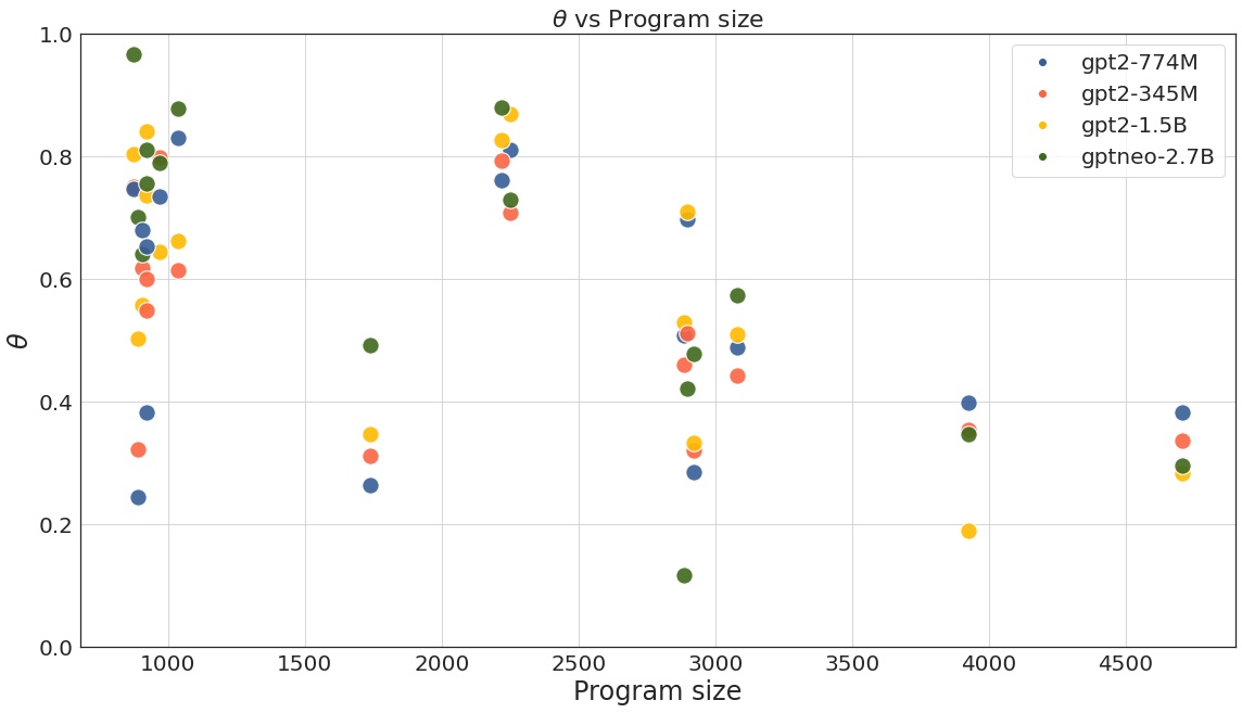
average performance vs program size (Figure 10): The programs generated for each task are of different sizes. The size of the program (number of characters in the program text) affects how easily it can be generated. For instance, the number of tokens transformer models can generate is bounded by their context window. We expect model performance to falter as the size of the program to generate increases.
- 2.
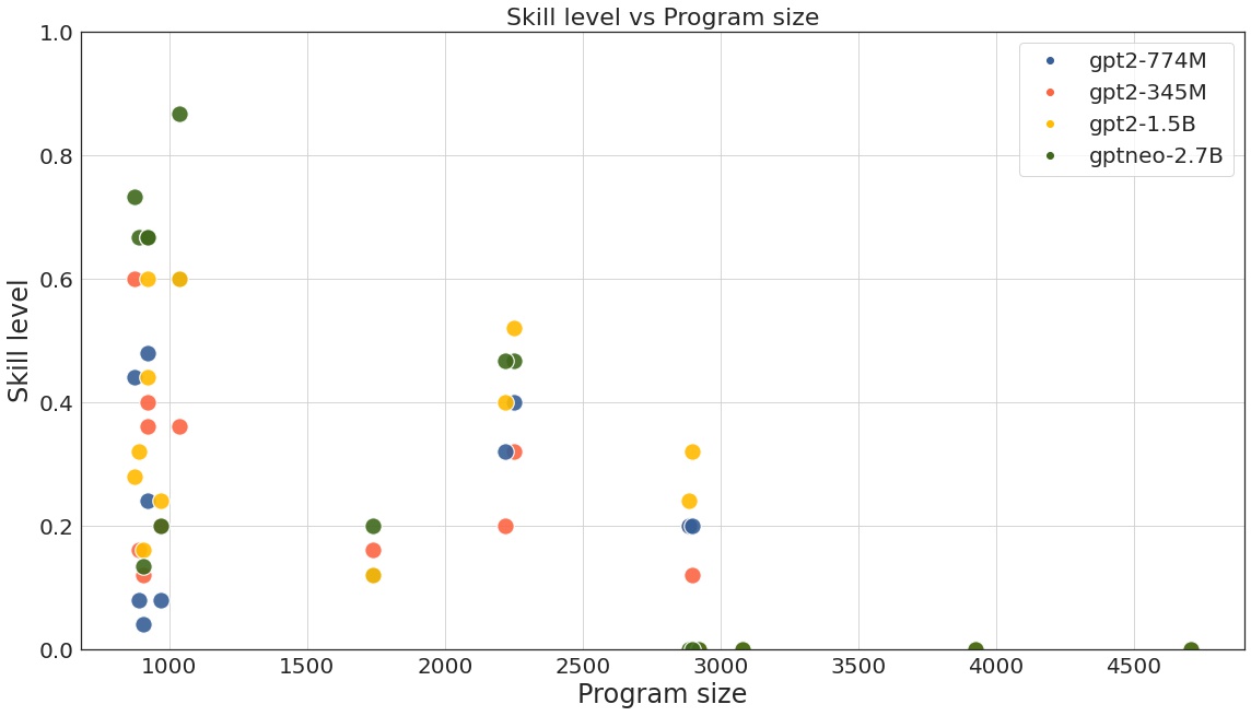
skill levels vs program size (Figure 11): The skill of an intelligence system is its ability to consistently generate correct programs to solve tasks in a given domain. In addition to performance, a measure of the system’s skill in a particular domain helps contextualize its potential for real-world use. When choosing an intelligence system to deploy in real-world tasks, we would prefer a system that generates correct programs more often.
- 3.
average performance vs number of training samples (Figure 12): The g-index penalizes increments in training samples, but rewards improvements in performance. We expect that the ideal system with a high g-index would occur at an optimal tradeoff between these two quantities.
- 4.
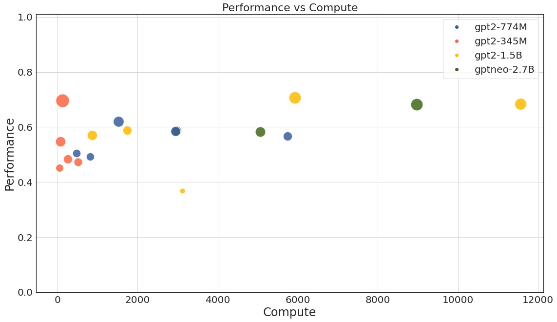
average performance vs compute used (Figure 13): The g-index penalizes high compute usage, but rewards improvements in performance. Compute is measured in terms of available compute power and training time, so systems that use multiple processors in parallel are penalized accurately. We expect the ideal system with a high g-index would occur at an optimal tradeoff between compute usage and performance.

| Model Name | # Training Samples | Compute Used44 4 f1 | g-index | ||
| 1. | GPT2-345M | 2560 | 127.530 | 0.697 | 7902.972+ |
| 2. | GPT Neo-2.7B | 2560 | 8969.100 | 0.682 | 6421.049 |
| 3. | GPT2-1.5B | 5120 | 5927.400 | 0.708+ | 6390.314 |
| 4. | GPT2-1.5B | 10240+ | 11563.320+ | 0.683 | 6006.261 |
| 5. | GPT2-774M | 2560 | 1516.640 | 0.620 | 4872.334 |
| 6. | GPT Neo-2.7B | 1280- | 5063.380 | 0.582 | 4476.680 |
| 7. | GPT2-345M | 1280- | 74.750- | 0.547- | 4399.190 |
| 8. | GPT2-774M | 5120 | 2941.941 | 0.585 | 4070.117- |
Different intelligence systems may obtain the best measurement at any individual component of the g-index . However, the best-performing system may not be the most resource-efficient, and vice-versa. The ideal system would be one that has the right combination of priors, experience, sample-efficiency, and maximal performance. Table 1 shows the top 8 models according to their g-index values, along with the models’ best component scores.
5 Flatland - a toy environment for the g-index
While the evaluation setup in Subsection 2.1 maps well to real-world tasks, the development of new learning methods will require toy environments with simpler program spaces and diverse task specifications. Since the g-index rewards sample-efficiency and performance on tasks of high generalization difficulty, new methods that score a high g-index within these environments will help surface insights for real-world tasks. Recent efforts in program synthesis use visual examples as training input to the system, such as images [45, 54] or video [46, 68]. To examine the g-index in such cases, we construct a toy environment called flatland, where intelligence systems must infer the correct program to draw shapes in an image.

The evaluation setup for flatland is similar to Section 2 and is described below55 5 Code available at https://github.com/mayahq/flatland :
- •
The task specified to the intelligence system is a 128x128 binary image. Each image contains shapes drawn using the commands loop, move, and turn as primitives.
- •
The program spec generated by can be expressed in a flow-based syntax, LISP expressions, or as JSON similar to programs for real-world tasks. Figure 14 shows an example. We use the turtle graphics library in Python [64] (similar to LOGO [8]) to draw the images from the DAG program specification. The DAG program is converted into a JSON list of primitives for comparison.
- •
The curriculum for consists of images and the corresponding DAG programs that generate them. flatland has in-built data augmentation to create programs with slight variations from an existing program.
- •
The scoring function evaluates the output of to the ideal program with a match-based metric that calculates the largest common subsets between the two lists. The largest common subset is computed via an association graph, similar to Subsection 2.4.
- •
The generalization difficulty of a task with the ideal program is computed by finding the nearest neighbor of in , similar to Subsection 2.5. Figure 15 shows some test samples along with their domain distance from a curriculum of just lines and circles.

Figure 15: Samples from the training and test sets for flatland. The training set consists of various images containing one to five circles or lines. Above each test sample we display its domain distance from the training set.
With flatland, we wish to examine intelligence systems by their g-index values in a controlled environment, so that we can test which learning methods generalize well when some constraints are relaxed. We also hope to improve the g-index definition by varying the evaluation setup itself. In the flatland environment, every aspect of program synthesis can be controlled and tested:
- •
The flatland environment currently provides programs that produce images, but this can be changed to accompany the image with text, or even use video. The program can be expressed in a flow-based syntax, or with LISP expressions, or also as JSON. This can help test synthesis methods that depend on different modalities.
- •
The DAG programs in flatland currently consist of three primitives loop, move, and turn. By varying the base set of primitives, we can attempt to find an ideal combination with which a system can learn to express the widest range of programs.
- •
The primitives in flatland can be combined to draw shapes, which can further be combined to produce more complex drawings. Thus new programs can be created via reuse and composition of existing programs, while keeping the program text minimal. This hierarchical composability could help create more flexible learners which build concepts on top of existing concepts to synthesize programs.
- •
flatland has in-built data augmentation to create programs with slight variations from an existing program, allowing the generation of arbitrarily large datasets on demand. As flatland programs are structurally similar to those used for real-world tasks (see Figure 14 and Figure 2), this could help assess the format, quantity, and diversity of training data that will be needed if a system has to adapt to tasks in the real world.
6 Summary and Future Directions
In this paper, we describe an experiment framework to obtain a quantitative measurement of skill-acquisition efficiency of machine intelligence systems. We model the intelligence system to accept a wide range of real-world tasks specified in natural language and synthesize programs representable as directed acyclic graphs in a flow-based programming syntax. We define a match-based metric to compare the DAG structures of two given programs to score the performance of the system, and use this metric to measure the generalization difficulty of any task provided to the system. We formulate the g-index benchmark and show that its changes with respect to dataset size, available compute, and performance align with intuitive expectations of an intelligence system with high generalization power. We then measure and compare the g-index scores of some fine-tuned transformer models and estimate their suitability for general-purpose intelligence systems. Finally, we provide a toy environment with a relaxed set of constraints to examine potential designs and improvements to the g-index .
While the g-index benchmark shifts the evaluation of intelligence systems into a quantitative context akin to skill-based evaluations, it is not yet a complete measure of general machine intelligence. However, we believe that future evaluations of intelligence systems will require a similar framework, one that reflects the potential real-world use of such systems. Over the course of our experiments, we have found some possible directions for improving the g-index measurement. We describe these possibilities and their effects below.
The evaluation framework can be improved to represent more real-world use cases for a machine intelligence system. The task specification can be expanded to include different natural languages, audio, video, and input-output examples. The task may even be specified in parts across an interaction between a human and the system [60]. Flow-based programs face limitations with maintaining state, so there is potential for improving the language of synthesized programs to account for multi-stage tasks. It is also possible to create more nodes with new functionality, enabling the construction of larger, diverse datasets of task specifications and their associated programs. With larger datasets, better data augmentation techniques can be built to generate reference programs to evaluate tasks. As more nodes are designed and flow-based programs grow larger, the subgraph isomorphism computation with may slow down, and the chance of program aliasing issues may also increase. In such cases, we may also need to use functional correctness like [63] to score the programs synthesized by the system.
With a given a set of tasks, the components of the g-index such as compute and domain distance can be refined by testing with a wider variety of intelligence systems, to ensure that the g-index value accurately represents their capabilities. Additionally, since the intelligence systems in our framework are evaluated on real-world tasks, human feedback can be incorporated when attempting to understand or improve the calculation of these components.
After calculating the scores for a wide range of systems, the g-index formula would need to be updated with additional specifications. If a system’s g-index score is unnaturally high, perhaps the system actually exhibits high skill-acquisition efficiency, or the formula contains some poorly specified variables which unfairly portray the system’s ability. For example, we consider the weightage for the priors encoded in the system ( in Equation 8) to be a constant neglible value for the current set of experiments that use transformer models fine-tuned from pre-trained weights. When comparing the g-index of a fine-tuned model to a model trained from scratch, the priors/compute tradeoff would be different, but it is not clear how such differences can be measured. Going further, it is difficult to quantify the benefit of priors like hyperparameters, data preprocessing, hardcoded rules and initial primitives in a manner that translates fairly across different kinds of intelligence systems. Perhaps the weight of some priors can be calculated by comparing the system’s performance with and without the prior:
| (10) |
The arrangement of Equation 10 along with the levels of generalization discusssed in Subsection 3.3 leads to an interesting question. When comparing machine intelligence with human intelligence, given that human beings have had thousands of years to build priors, should human priors have a weight of ? Is it necessary to compare the built-in priors of humans with that of machines?
The overarching aim of this work is not only to propose a method-agnostic way to compare different techniques quantitatively, but also to spark a conversation on the relative merits of different approaches that could help reach higher levels of general machine intelligence. While we don’t expect our g-index definition to be complete, it anchors a previously abstract concept in a mathematical formulation made up of quantities that can be measured during experiments. The flow-based programming language we propose can act as a common language to express and compare programs of real-world utility across a wide variety of domains. The g-index explicitly rewards resource-efficiency, which we hope incentivises sustainable ways of achieving generalization which do not rely on unlimited amounts of compute and data. A good outcome of this would be the patronage and competitive development of new methods and technologies to reach higher g-index levels, similar in spirit to the Hutter compression challenge [65]. Ultimately, our belief is that intelligent machines will only be able to contribute to real technological progress when they can learn how do more from less, not the other way around.
References
- [1] David Wechsler “The measurement of adult intelligence” Williams & Wilkins Co, 1944
- [2] Alan Turing and J Haugeland “Computing machinery and intelligence” MIT Press Cambridge, MA, 1950
- [3] Alfred Binet and Theophile Simon “The development of intelligence in children.” Appleton-Century-Crofts, 1961
- [4] M Quillian and Marvin Minsky “Semantic information processing”, 1968
- [5] RJ Waldinger and RCT LEE “A step toward automatic program writing” In Proc. Int. Joint Conf. on Artificial Intelligence (Washington DC), 1969, pp. 241–252
- [6] Saul Amarel “Representations and modeling in problems of program formation” Rutgers University, 1970
- [7] J Morrison “Data responsive modular, interleaved task programming system” In IBM Technical Disclosure Bulletin 13.8, 1971, pp. 2425–2426
- [8] Wallace Feurzeig and George Lukas “LOGO—A programming language for teaching mathematics” In Educational Technology 12.3 JSTOR, 1972, pp. 39–46
- [9] Harry Barrow and BURSTALL RM “Subgraph isomorphism, matching relational structures and maximal cliques.”, 1976
- [10] Julian Ullmann “An algorithm for subgraph isomorphism” In Journal of the ACM (JACM) 23.1 ACM New York, NY, USA, 1976, pp. 31–42
- [11] Phillip Summers “A methodology for LISP program construction from examples” In Journal of the ACM (JACM) 24.1 ACM New York, NY, USA, 1977, pp. 161–175
- [12] Dexter Kozen “A clique problem equivalent to graph isomorphism” In ACM SIGACT News 10.2 ACM New York, NY, USA, 1978, pp. 50–52
- [13] John Searle “Minds, brains, and programs” In Behavioral and brain sciences 3.3 Cambridge University Press, 1980, pp. 417–424
- [14] Shahid. Bokhari “On the mapping problem” In IEEE Trans. Computers 30.3, 1981, pp. 207–214
- [15] Gregory Chaitin “Gödel’s theorem and information” In International Journal of Theoretical Physics 21.12 Springer, 1982, pp. 941–954
- [16] Marvin Minsky “Semantic information processing” CUMINCAD, 1982
- [17] B Chandrasekaran “What kind of information processing is intelligence?” In The foundation of artificial intelligence—a sourcebook, 1990, pp. 14–46
- [18] Linda. Gottfredson “Mainstream science on intelligence: An editorial with 52 signatories, history, and bibliography” Special Issue Intelligence and Social Policy In Intelligence 24.1, 1997, pp. 13–23 DOI: https://doi.org/10.1016/S0160-2896(97)90011-8
- [19] Daniel Dennett “Brainchildren: Essays on designing minds” MIT Press, 1998
- [20] Yann LeCun “The MNIST database of handwritten digits” In http://yann. lecun. com/exdb/mnist/, 1998
- [21] Arthur Jensen “The g factor: The science of mental ability” In Psicothema 11.2 Colegio Oficial de Psicólogos del Principado de Asturias, 1999, pp. 445–446
- [22] Kishore Papineni, Salim Roukos, Todd Ward and Wei-Jing Zhu “Bleu: a method for automatic evaluation of machine translation” In Proceedings of the 40th annual meeting of the Association for Computational Linguistics, 2002, pp. 311–318
- [23] Selmer Bringsjord, Paul Bello and David Ferrucci “Creativity, the Turing test, and the (better) Lovelace test” In The Turing Test Springer, 2003, pp. 215–239
- [24] Luiz Oliveira and Robert Sabourin “Support vector machines for handwritten numerical string recognition” In Ninth International Workshop on Frontiers in Handwriting Recognition, 2004, pp. 39–44 IEEE
- [25] Daniel Keysers “Comparison and combination of state-of-the-art techniques for handwritten character recognition: topping the mnist benchmark” In arXiv preprint arXiv:0710.2231, 2007
- [26] Shane Legg and Marcus Hutter “Universal intelligence: A definition of machine intelligence” In Minds and machines 17.4 Springer, 2007, pp. 391–444
- [27] VN Manjunath, G Hemantha and S Noushath “Unconstrained Handwritten Digit Recognition: Experimentation on MNIST Database” In Advances In Pattern Recognition World Scientific, 2007, pp. 140–143
- [28] Cassio Pennachin and Ben Goertzel “Contemporary Approaches to Artificial General Intelligence” In Artificial General Intelligence Berlin, Heidelberg: Springer Berlin Heidelberg, 2007, pp. 1–30 DOI: 10.1007/978-3-540-68677-4˙1
- [29] Ming Li and Paul Vitányi “An introduction to Kolmogorov complexity and its applications” Springer, 2008
- [30] Jia Deng et al. “Imagenet: A large-scale hierarchical image database” In 2009 IEEE conference on computer vision and pattern recognition, 2009, pp. 248–255 Ieee
- [31] J. Searle “Chinese room argument” revision #66188 In Scholarpedia 4.8, 2009, pp. 3100 DOI: 10.4249/scholarpedia.3100
- [32] J Morrison “Flow-Based Programming: A new approach to application development” CreateSpace, 2010
- [33] Douglas Crockford “Json” In ECMA International, 2012
- [34] David Dowe and José Hernández-Orallo “IQ tests are not for machines, yet” Elsevier, 2012
- [35] Alex Krizhevsky, Ilya Sutskever and Geoffrey Hinton “Imagenet classification with deep convolutional neural networks” In Advances in neural information processing systems 25, 2012, pp. 1097–1105
- [36] Mark Riedl “The Lovelace 2.0 test of artificial creativity and intelligence” In arXiv preprint arXiv:1410.6142, 2014
- [37] Mohammad Raza, Sumit Gulwani and Natasa Milic-Frayling “Compositional program synthesis from natural language and examples” In Twenty-Fourth International Joint Conference on Artificial Intelligence, 2015
- [38] Emilio Parisotto et al. “Neuro-Symbolic Program Synthesis”, 2016 arXiv:1611.01855 [cs.AI]
- [39] Felipe Pezoa et al. “Foundations of JSON schema” In Proceedings of the 25th International Conference on World Wide Web, 2016, pp. 263–273 International World Wide Web Conferences Steering Committee
- [40] José Hernández-Orallo “Evaluation in artificial intelligence: from task-oriented to ability-oriented measurement” In Artificial Intelligence Review 48.3, 2017, pp. 397–447 DOI: 10.1007/s10462-016-9505-7
- [41] Xi Lin et al. “Program synthesis from natural language using recurrent neural networks” In University of Washington Department of Computer Science and Engineering, Seattle, WA, USA, Tech. Rep. UW-CSE-17-03-01, 2017
- [42] Pengcheng Yin and Graham Neubig “A Syntactic Neural Model for General-Purpose Code Generation”, 2017 arXiv:1704.01696 [cs.CL]
- [43] Rudy Bunel et al. “Leveraging Grammar and Reinforcement Learning for Neural Program Synthesis” In CoRR abs/1805.04276, 2018 arXiv: http://arxiv.org/abs/1805.04276
- [44] Jacob Devlin, Ming-Wei Chang, Kenton Lee and Kristina Toutanova “Bert: Pre-training of deep bidirectional transformers for language understanding” In arXiv preprint arXiv:1810.04805, 2018
- [45] Kevin Ellis, Daniel Ritchie, Armando Solar-Lezama and Joshua. Tenenbaum “Learning to Infer Graphics Programs from Hand-Drawn Images”, 2018 arXiv:1707.09627 [cs.AI]
- [46] Shao-Hua Sun, Hyeonwoo Noh, Sriram Somasundaram and Joseph Lim “Neural program synthesis from diverse demonstration videos” In International Conference on Machine Learning, 2018, pp. 4790–4799 PMLR
- [47] Alex Wang et al. “GLUE: A multi-task benchmark and analysis platform for natural language understanding” In arXiv preprint arXiv:1804.07461, 2018
- [48] François Chollet “On the Measure of Intelligence” In CoRR abs/1911.01547, 2019 arXiv: http://arxiv.org/abs/1911.01547
- [49] Jie Hu et al. “Squeeze-and-Excitation Networks”, 2019 arXiv:1709.01507 [cs.CV]
- [50] Sumith Kulal et al. “Spoc: Search-based pseudocode to code” In arXiv preprint arXiv:1906.04908, 2019
- [51] Alec Radford et al. “Language models are unsupervised multitask learners” In OpenAI blog 1.8, 2019, pp. 9
- [52] Lucas Beyer et al. “Are we done with imagenet?” In arXiv preprint arXiv:2006.07159, 2020
- [53] Tom Brown et al. “Language models are few-shot learners” In arXiv preprint arXiv:2005.14165, 2020
- [54] Kevin Ellis et al. “Dreamcoder: Growing generalizable, interpretable knowledge with wake-sleep bayesian program learning” In arXiv preprint arXiv:2006.08381, 2020
- [55] Leo Gao et al. “The Pile: An 800GB Dataset of Diverse Text for Language Modeling” In arXiv preprint arXiv:2101.00027, 2020
- [56] Marie-Anne Lachaux, Baptiste Roziere, Lowik Chanussot and Guillaume Lample “Unsupervised translation of programming languages” In arXiv preprint arXiv:2006.03511, 2020
- [57] Shuo Ren et al. “Codebleu: a method for automatic evaluation of code synthesis” In arXiv preprint arXiv:2009.10297, 2020
- [58] Kensen Shi, David Bieber and Rishabh Singh “TF-Coder: Program Synthesis for Tensor Manipulations”, 2020 arXiv:2003.09040 [cs.PL]
- [59] Thomas Wolf et al. “Transformers: State-of-the-Art Natural Language Processing” In Proceedings of the 2020 Conference on Empirical Methods in Natural Language Processing: System Demonstrations Online: Association for Computational Linguistics, 2020, pp. 38–45 URL: https://www.aclweb.org/anthology/2020.emnlp-demos.6
- [60] Jacob Austin et al. “Program Synthesis with Large Language Models”, 2021 arXiv:2108.07732 [cs.PL]
- [61] Henri Bergius “NoFloJS: Flow-based programming for Javascript”, 2021 URL: https://noflojs.org/
- [62] Sid Black et al. “GPT-Neo: Large Scale Autoregressive Language Modeling with Mesh-Tensorflow”, 2021 URL: http://github.com/eleutherai/gpt-neo
- [63] Mark Chen et al. “Evaluating Large Language Models Trained on Code”, 2021 arXiv:2107.03374 [cs.LG]
- [64] Python Foundation “turtle graphics in Python 3.7.12”, 2021 URL: https://docs.python.org/3.7/library/turtle.html
- [65] Marcus Hutter “Hutter Prize: Human Knowledge Compression Contest”, 2021 URL: http://prize.hutter1.net/
- [66] Vadim Liventsev, Aki Härmä and Milan Petkovic “BF++: a language for general-purpose neural program synthesis” In CoRR abs/2101.09571, 2021 arXiv: https://arxiv.org/abs/2101.09571
- [67] OpenJS “Node-RED: Low-code programming for event-driven applications”, 2021 URL: https://nodered.org/about/
- [68] Tianmin Shu et al. “AGENT: A Benchmark for Core Psychological Reasoning” In arXiv preprint arXiv:2102.12321, 2021
Appendix A Sample Task Domains and Descriptions
| Domain Name | Example Text Prompt | Nodes | Program size(chars) | Best Avg Performance | Skill Level ** |
| template-slider | Two sliders with values ranging from 0 to 20 changing in steps of 2 | 6 | 1493 | 1.00 | 1.00 |
| template-form | Create a form with fields for entering Name, Benchmark Score and Date of Submission | 5 | 1473 | 1.00 | 1.00 |
| cron-reminder | Set a reminder for ’Send Daily Digest’ every first day of the week, Tuesday through Saturday, only in January | 3 | 935 | 1.00 | 1.00 |
| cron-schedule | Repeat At 48, 9, 14, 7, 6, 56, 46, 39, 15, 3, 37, and 30 minutes past the hour, between 05:00 AM and 08:59 PM, on day 1,4,8 and 9 of the month, only on Tuesday, every 3 months, November through December | 3 | 896 | 1.00 | 1.00 |
| On Facebook, when user says ’Hello’, reply with ’Hi there! How can I help you?’, and when user says ’Bye’, reply with ’Goodbye!’ | 8 | 2253 | 1.00 | 1.00 | |
| gmail-send | Send email with body ’Upcoming Meeting’ and subject ’Discuss paper appendices’ to email alpha@beta.com | 12 | 4708 | 0.63 | 0.00 |
| google-search | Search Google for ’How to make tables on LaTeX’ and scrape results | 9 | 2963 | 0.60 | 0.0 |
| googlesearch-to-csv | Search Google for ”Papers on measuring general intelligence”, scrape results and put into singularity.csv | 12 | 3894 | 0.59 | 0.0 |
| http | Create a HTTP POST endpoint called /agents | 4 | 857 | 1.0 | 1.0 |
| telegram-2-reply | Reply ’Yes, detective?’ to ’Sonny!’, and ’Of course, Dave’, to ’Open the pod bay doors’ on Telegram | 8 | 2148 | 1.0 | 1.0 |
| telegram-3-reply | On Telegram, when user says ’Are friends electric?’, reply with ’No, only sheep’, when user says ’How deep is your love?’ reply with ’6.5 meters’, and when user says ’Is that all there is?’, reply with ’Yes’ | 10 | 2910 | 1.0 | 1.0 |
| Obtain tweets about the topic #Alignment | 4 | 892 | 1.0 | 1.0 | |
| url-skill | Create a skill called ’Open LessWrong’ which opens url https://www.lesswrong.com/ | 4 | 1067 | 1.0 | 1.0 |
| youtube-pause | Pause Youtube video | 3 | 919 | 1.0 | 1.0 |
| youtube-play | Find and play Vivaldi Four Seasons on Youtube | 9 | 3050 | 0.89 | 0.0 |
| youtube-resume | Resume Youtube Video | 3 | 916 | 1.0 | 1.0 |
Appendix B Node Library
| Categories | Description | Node Types |
|---|---|---|
| common utility | Custom triggers, catch bugs, add comments | inject, debug, complete, catch, status, link in, link out, comment |
| functional | Change, switch, filter or delay the passed message object or add custom logic to manipulate it | function, switch, change, range, template, delay, trigger, exec, filter |
| network | Different kinds of network interfaces to send and receive data | mqtt in, mqtt out, http in, http response, http request, websocket in, websocket out, tcp in, tcp out, tcp request, udp in, udp out |
| sequence | Manipulate sequences and arrays in predictable ways | split, join, sort, batch |
| parser | Parse data from different files into fixed formats for easy processing | csv, html, json, xml, yaml |
| storage | Read and write to files | file, file in, watch |
| dashboard | Make dynamic dashboards with forms and charts by linking UI elements to other pieces of logic | button, dropdown, switch, slider, numeric, text input, date picker, colour picker, form, text, gauge, chart, audio out, notification |
| browser-automation | Interact with the browser to navigate the web and scrape websites | open, click, type, press, execute function, find tab, scrape, query, bookmark |
| spotify-automation | Integrate with spotify and control music played on any device | play, search, control playback, get playback state, control playlist |
| gdrive-automation | Search through, read, export and append to files in on your google drive | search gdrive, gsheet append, gdrive-export-file |
| scheduling | Schedule triggers to run events at any fixed interval | schedule-trigger |
| zoom-automation | Create, view and attend zoom meetings | create-meeting, list-meetings, list-meetings-registrants |
| system utilities | Interact with various system level utilities on the desktop | clipboard-add, clipboard-get, open-target, file-search, desktop-notify |
| stock-automation | Buy, sell and view orders on the stock market via third party API | submit-order, get-order, get-bars, get-account |
| home-automation | Control lights and switches remotely | light-control, switch-control |
Appendix C Calculating via subgraph isomorphism
When computing the value of between two arbitrary DAGs, we
use the similarity function to compare individual nodes, and
account for structural similarity by computing the largest subgraph common to both DAGs.
This is known as the maximum common edge subgraph problem, [14],
an extension of the subgraph isomorphism problem [10]. In this
section, we explain in detail the calculation of outlined in
Subsubsection 2.4.3.
Two graphs and are isomorphic to each oher () if there exists a bijection that preserves the graph structure:
| (3) |
We need to find the largest subgraphs and that are isomorphic to each other (), and the isomorphism between the nodes of the two subgraphs. We obtain these by constructing the association graph and finding a maximum clique in . The association graph for given graphs , contains the vertices : a vertex associates a node to a node with their node similarity . Only nodes of the same type are considered for association:
| (11) |
An edge in connects a vertex to another vertex provided the below structure-preserving condition is satisfied (note the resemblance to Equation 3):
| (12) |
It can be shown that finding a maximum clique66 6 Note that the node similarities are used to filter out elements from and when computing the maximum clique (a node-weight maximum clique is computed). in the association graph is equivalent to finding the largest common subgraph between and [9, 12]. Once a maximum clique in has been obtained, we can construct the common subgraphs and . Since nodes in the DAGs and cannot have self-loops, Equation 12 ensures that any clique in the association graph will always provide a one-to-one mapping between the corresponding vertices of and . If
is the maximum clique in the association graph , then
are the required largest common subgraphs. The maximum subgraph isomorphism is the mapping expressed via the pairs in the elements of of the clique .
Thus with we can compute the value of the metric as provided in Equation 5:
| (5) | ||||
| (13) |
We note that is 1 when either of the DAGs are empty, and reduces to the node similarity function in Equation 2 when both have one vertex and zero edges. also satisfies the constraints in Equation 1.
- •
is bounded:
(14) - •
is symmetric because the node similarities are symmetric, and finding the largest common subgraph between two graphs is also symmetric: since , we can construct a bijection between and , and use its inverse for the symmetric case.
- •
If ,
(15) - •
If ,
(16)