Local tensor-network codes

Tensor networks BC17 have proved useful in quantum error correction, primarily for decoding FP14; BSV14; FP14a; Darmawan17; Darmawan18; CF18; FHM20; Chubb21. In FP14, Ferris and Poulin created a decoder by representing the encoding circuit of the code as a tensor network for circuits that were similar to the MERA tensor network. Using a different approach, the surface code was decoded by contracting a two-dimensional tensor network in BSV14. This method was applied to several different noise models CF18; TDC19; TBF18 and also expanded to general codes with local stabilizers in two dimensions Chubb21. Non unitary and correlated noise were decoded for the surface code using a PEPO representation of the state Darmawan17; Darmawan18. Tensor networks have also been instrumental for constructing holographic error correcting codes FYH15; LS15; HNQ16; Evenbly17; HMBS18; BO18; JGP19; JGP19a; KC19; OS20; MFG20.

More recently, “tensor-network codes” FHM20; FHM20b were introduced, which use tensors to describe stabilizer codes. This allows one to easily construct new larger codes by connecting many tensors (i.e., by contracting tensor indices) to form a new code. Trivial examples are concatenated and convolutional codes, but more interesting examples include holographic codes FHM20. In principle, there is no restriction on the geometry of the tensor network, though some geometries lend themselves to efficient tensor contraction, which naturally produces an efficient decoder FHM20.

In this work, we build up more new tensor-network codes. For example, we look at topological codes, where we see that surface codes are very simple examples of tensor-network codes, as is the colour code. We also show how to use tensor networks to calculate distances for stabilizer codes. After first applying this to some simple examples of stabilizer codes, we then use this distance calculator to modify the surface code to find a code with the same distance but with fewer minimal-weight logical operators. This modified code has an improved success probability of correcting depolarizing noise of up to $2\%$. This works simply by substituting the (non CSS) five-qubit code tensor into the tensor network describing the surface code.

In this paper, we focus on stabilizer codes Gottesman97; Gottesman09; NielsenChuang; Roffe19, in which stabilizers and logical operators are elements of $\mathcal{G}_{n}$, which is the $n$-qubit Pauli group. The group $\mathcal{G}_{n}$ comprises all operators of the form $z\sigma^{i_{1}}\otimes...\otimes\sigma^{i_{n}}$, with $z\in\{\pm 1,\pm i\}$. Here, we are denoting the identity and three Pauli operators via $\sigma^{0}=\openone$, $\sigma^{1}=X$, $\sigma^{2}=Y$ and $\sigma^{3}=Z$.

The codespace, which is the subspace of the Hilbert space used to encode logical information, is fully determined by the stabilizers, an abelian group of Pauli operators, i.e., $\mathcal{S}\subset\mathcal{G}_{n}$. The codespace is determined by the fact that every state $|\psi\rangle$ in the codespace satisfies $S|\psi\rangle=|\psi\rangle$ for all stabilizers $S\in\mathcal{S}$. If we denote the number of independent generators of $\mathcal{S}$ by $r$, then the dimension of the codespace is $2^{n-r}$, which corresponds to $k=n-r$ encoded logical qubits NielsenChuang. We denote generators by $S_{i}$.

The logical operators of the code generate a group $\mathcal{L}\subset\mathcal{G}_{n}$, which is non-abelian. One set of generators for the group is the $k$ $Z$-type and $k$ $X$-type operators. (By $Z$-type and $X$-type, we mean that these operators are canonically conjugate to each other, not that they only consist of $\sigma^{1}$ or $\sigma^{3}$ Pauli operators.) We denote these by $Z_{\alpha}$ and $X_{\alpha}$ respectively, with $\alpha\in\{1,..,k\}$. These operators commute with all stabilizers, while anticommuting pairwise, i.e., $X_{\alpha}Z_{\beta}=(-1)^{\delta_{\alpha\beta}}Z_{\beta}X_{\alpha}$.

It will be useful to also consider the (abelian) group of operators called pure errors (a.k.a. destabilizers) $\mathcal{P}\subset\mathcal{G}_{n}$. This group is defined by $n-k$ operators $P_{i}$ which satisfy $P_{i}S_{j}=(-1)^{\delta_{ij}}S_{j}P_{i}$ and $P^{2}_{i}=\openone$. The Pauli group on $n$ physical qubits is generated by products of $P_{i}$, $S_{i}$, $X_{\alpha}$ and $Z_{\alpha}$.

Finally, during error correction, we measure each of the stabilizer generators (which have eigenvalues $\pm 1$), giving the error syndrome. This is a length-$r$ vector $\vec{s}$ of the measurement outcomes, with $s_{i}=0$ if the error commuted and $s_{i}=1$ if the error anticommuted with stabilizer $S_{i}$. Finding the optimal correction operator given the syndrome is extremely difficult in general HG11; IP13, though some algorithms work well for some codes (e.g., minimum-weight perfect matching for the surface code). It is always straightforward to find an error consistent with a given syndrome by using the pure errors, i.e., the operator $P(\vec{s}\,)=\prod_{i}P^{s_{i}}_{i}$ gives rise to the syndrome $\vec{s}$. But quantum codes are degenerate, meaning multiple different errors can have the same syndrome, e.g., $P(\vec{s}\,)$ and $P(\vec{s}\,)S$ for any stabilizer $S$ will give rise to the same error syndrome.

As introduced in FHM20, we represent small “seed” stabilizer codes by tensors and use them to build up bigger stabilizer codes. This works as follows. We can represent Pauli operators by strings of integers, so the operator $XZZX\openone=\sigma^{1}\sigma^{3}\sigma^{3}\sigma^{1}\sigma^{0}$ would be represented by the string $(1,3,3,1,0)$.

For a stabilizer code with $n$ physical and $k$ logical qubits, we define the rank-$n$ tensor

for each logical operator $L$. Here the indices $g_{j}\in\{0,1,2,3\}$, and $\mathcal{S}L$ is the set of all operators $SL$ with $S\in\mathcal{S}$. In other words, $\mathcal{S}L$ is the coset of $\mathcal{S}$ with respect to logical $L$. We can also think of $T(L)_{g_{1},...,g_{n}}$ as the indicator function for all operators in the class $L$.

As an example, $T(\openone)_{g_{1},...,g_{n}}$ describes the stabilizer group, as it is non zero only if $\sigma^{g_{1}}\otimes...\otimes\sigma^{g_{n}}$ corresponds to a stabilizer. This does not include the signs of the stabilizers, though once these are fixed for a set of generators, then they are fully determined for the rest of the group. Also, for a stabilizer code that has only a single logical qubit, the tensor $T(X)_{g_{1},...,g_{n}}$ describes the coset corresponding to the logical $X$ operator.

As explained in FHM20, contracting seed tensors generates larger codes, which come with a natural tensor-network decoder. A useful idea then is to start with a tensor-network geometry that is efficiently contractible and use this to construct codes that we know we can decode efficiently since we can contract the tensor network. We can then vary the code tensors within this geometry to search for good codes.

To see how to contract code tensors to get new stabilizer codes is straightforward. First, the tensor describing a tensor product of two stabilizer codes is just the product of the code tensors:

Second, we contract two indices (say $g_{1}$ and $h_{1}$ above). To understand when the resulting tensor describes a bona fide stabilizer code, we look at the more general case of contracting two indices of a code tensor. Take code tensor $T(L)_{j_{1},...,j_{n}}$ with $n$ physical qubits and $k$ logical qubits. Suppose we contract two indices (take the first two indices for simplicity), i.e.,

It is straightforward to check if the left hand side is a code tensor describing a stabilizer code, as shown in more detail in appendix A. In short, a sufficient condition ensuring that the resulting tensor also describes a stabilizer code is if we can find two stabilizers of the original code $S_{1}$ and $S_{2}$ that have the following form. Writing $S_{1}=\sigma^{j_{1}}\otimes\sigma^{j_{2}}\otimes\sigma^{j_{3}}\otimes...$ and $S_{2}=\sigma^{i_{1}}\otimes\sigma^{i_{2}}\otimes\sigma^{i_{3}}\otimes...$, we require that $i_{1}\neq i_{2}$ and $j_{1}\neq j_{2}$. We also require that after taking their product $S_{1}S_{2}=\sigma^{k_{1}}\otimes\sigma^{k_{2}}\otimes\sigma^{k_{3}}\otimes...$ with $k_{1}\neq k_{2}$. This condition is sufficient but not necessary in some cases, as explained in appendix A. From a numerical perspective, two stabilizers satisfying the conditions above can be found quickly (in $O(n)$ time), and stabilizer generators and logical operators for the new stabilizer code can also be found quickly (also in $O(n)$ time).

With this formalism it is straightforward to build larger error correcting codes using smaller seed code tensors as building blocks. These tensor-network codes include many holographic codes as well as concatenated codes and generalized concatenated codes GSS09; WZG13. However, there is no restriction on the geometry of the network or the number of logical qubits.

Physically, in a photonic setting we can think of the contraction of two tensor indices as type-II fusion BR05; BBB21, where we are measuring $\sigma^{1}\otimes\sigma^{1}\otimes\openone...$ and $\sigma^{3}\otimes\sigma^{3}\otimes\openone...$.

In Figure 1 (a), we give an example of a simple tensor-network code composed of three five-qubit code tensors (see Table 1 for a description of the five-qubit code). This is a $[[8,3,3]]$ code, which is the maximum distance for a code with eight physical and three logical qubits Grassl21.

The tensor-network code construction naturally gives rise to an algorithm for computing the code distance. In fact, we can calculate more information: by contracting a tensor network, we generate a histogram of operators (logicals and/or stabilizers) according to their weight. If the tensor-network is efficiently contractible, then this histogram can be generated efficiently.

To see this, start by defining a weight tensor:

where the function weight returns the weight of a Pauli operator, i.e., the number of locations where it acts non trivially. To find the distribution of operator weights of a tensor-network code, we use the representation $T^{l_{1},...,l_{k}}_{g_{1},...,g_{n}}=T(L)_{g_{1},...,g_{n}}$, where $l_{i}=0,1,2,3$ indicates the logical identity, $X$, $Y$ and $Z$ operator on the $i$th logical qubit. Then the number of operators of each weight for each logical coset is given by

where repeated indices are summed. For example, $C_{w}^{0,...,0}$ is a list of the numbers of stabilizers of each weight. Then we calculate the distance of the code using

Here we sum over all logical cosets and then subtract the identity coset (the stabilizer group). The code distance is then given by the first value of the index $w$ for which $D_{w}\neq 0$.

On its own, this is not particularly useful, as the tensors $T$ or $W$ will become unwieldy for large $n$. However, we split $W$ into a product of smaller tensors by first generalizing it:

We note that $W_{w_{\mathrm{out}}}^{g_{1},...,g_{n}}=W_{w_{\mathrm{out}},0}^{g_{1},...,g_{n}}$. It follows that these tensors can be chained in a natural way.

We can chain these tensors in a way that mimics the tensor-network geometry of the original code. As a result if the original code tensor network can be contracted easily, so can the tensor network to calculate weights.

Let us consider a simple example. As shown in Figure 1 (b), we have contracted five code tensors, with one corresponding to the five-qubit code, and the rest corresponding to the purified five-qubit code (see Table 1), so there is a single logical qubit. By using our tensor-network method, we find the distribution of operator weights as shown in figure 1 (c). We see that the distance is five, so this is a $[[13,1,5]]$ code.

This is a promising new way to find code distances, provided we can contract the tensor network. Then a useful idea is to start with tensor-network geometries that we know we can easily contract and then iterate over different choices of seed code tensors to find high-distance codes. We can also look for codes that not only have high distance but also have many low-weight stabilizers. This method can also be expanded to find the distribution of logical operators by weight restricted to those of a certain form, e.g., those that have only identity and Pauli $Z$ components. This can be used to identify codes that are tailored to biased noise TDC19.

Let us end this section by noting that this distance calculation method is efficient for holographic codes (see appendix B), as well as for any code with simpler tensor networks, such as trees.

Maximum likelihood decoding is optimal, as it uses the syndrome to find the correction operator that is most likely to return the code to the correct code state. For general quantum codes, this is a very difficult computational task IP13. One method that works well for some codes uses tensor networks FP14; BSV14; CF18; FHM20; Chubb21.

We can write any error with syndrome $\vec{s}$ as $P(\vec{s}\,)SL$, where $P(\vec{s}\,)$ is the pure error corresponding to syndrome $\vec{s}$, and some $S\in\mathcal{S}$ and $L\in\mathcal{L}$. The key point is that $P(\vec{s}\,)SL$ has the same effect on the codespace regardless of which stabilizer $S$ appears. In contrast, different logicals $L$ will have different effects on the codespace. To find the optimal correction, we need to calculate

for each logical $L\in\mathcal{L}$. Here $\mathrm{prob}(P(\vec{s}\,)SL)$ is the probability that the error $P(\vec{s}\,)SL$ occurred. Then the best correction operator is $\overline{L}P(\vec{s}\,)$, where $\overline{L}=\argmax_{L}\chi(L,\vec{s}\,)$.

Using tensor-network codes, we should think of the noise distribution $\mathrm{prob}(P(\vec{s}\,)SL)$ as a tensor. To do this, we write $SL=\sigma^{g_{1}}\otimes...\otimes\sigma^{g_{n}}$ and $P(\vec{s}\,)=\sigma^{e_{1}}\otimes...\otimes\sigma^{e_{n}}$. Recall that $P(\vec{s}\,)$ is fixed by the syndrome. Then we define

For uncorrelated error models (e.g., i.i.d. depolarizing noise), this factorizes simply to a product of rank-one tensors: $\mathcal{E}(\vec{s}\,)^{g_{1},...,g_{n}}=p_{1}(\sigma^{e_{1}}\sigma^{g_{1}})\times...\times p_{n}(\sigma^{e_{n}}\sigma^{g_{n}})$, with $p_{i}(\sigma^{a_{i}})$ being the probability that the noise will cause $\sigma^{a_{i}}$ to act on qubit $i$.

Calculating $\chi(L,\vec{s}\,)$ involves contracting the code tensor with $\mathcal{E}$ to get

As we saw for the tensor-network distance calculator, this is useful if $T$ and $\mathcal{E}(\vec{s}\,)$ both factorize in a way that is amenable to contraction. This is made especially easy for i.i.d. noise, but correlated noise can also be handled in some cases if, e.g., it has a finite correlation length, as is the case for factored noise CF18.

There are some important examples where this decoding approach works well, such as (planar) surface codes BSV14, codes based on the MERA tensor network FP14, and holographic codes FHM20. It is also clear that such an approach would work well for concatenated or convolutional codes, but these already have efficient and exact decoders. Typically, this decoding method involves approximations, e.g., in BSV14 the two-dimensional tensor network was contracted using the MPS-MPO method, which uses bond-dimension truncation.

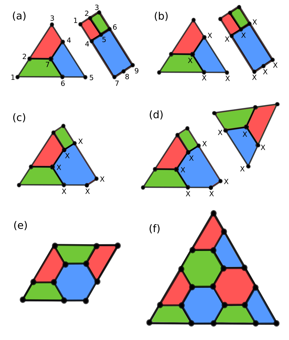
We view several important topological codes as tensor-network codes built from smaller codes. For example, the rotated surface code can be seen as a tensor-network code made of surface code fragments. This is constructed from bulk tensors corresponding to the five-qubit surface code with stabilizers in Table 2. The construction is most easily understood from Figure 2. Similarly one can construct the colour code, as described in appendix C, and the original (unrotated) surface code.

Consider a rotated $[[L^{2},1,L]]$ surface code with length $L$. The degeneracy of the lowest-weight logical operators is actually quite high and grows quickly with $L$, e.g., for $L=7$ it is already $896$, versus only $14$ for the original surface code with $L=7$. It seems natural that keeping distance and code size fixed, while lowering the degeneracy of the lowest-weight logical operators may be an interesting avenue to explore to find better performing codes.

We will do this by using the tensor-network representation of the rotated surface code and then changing some of the tensors. The simplest example is to replace the central tensor encoding the logical qubit by the $[[5,1,3]]$ non CSS five-qubit code tensor. We compare the operator weights for this modified code with that of the rotated surface code. For example, for a $7\times 7$ code, we see that both codes have the same size $n=49$ and the same distance $d=7$, but the rotated surface code has a degeneracy of the lowest-weight logical operators of $896$, whereas for the modified code, this is only $650$. This reduction in the number of low-weight logical operators will improve the error correction properties. Indeed, in Figure 3, we see that the modified code does perform somewhat better under depolarizing noise using the tensor-network decoder. The price we pay is some (four) of the stabilizers are modified to have higher weight, as shown in Figure 6 in appendix C. An interesting question is if this improvement persists in a fault-tolerant setting, where higher weight stabilizers increase the possibility for additional errors to creep in. Regardless, this general idea also offers the possibility of optimization strategies to find good codes, e.g., using reinforcement learning.

Our main result is a method that creates general tensor-network codes on graphs. This also comes with a tensor-network based method to calculate code distances, as well as the full distribution of operator (logical and stabilizer) weights. For example, we can search for good tensor-network codes by iterating over different contractions of (perhaps randomly chosen) code tensors to find the highest distance code, and then among codes with high distance, we can choose one that has the lowest number of minimal-weight logical operators. This is precisely what we did to find the modified surface code in section VI. By replacing the central code tensor with a five-qubit code tensor with its legs randomly permuted, we found a modification of the rotated surface code with the same distance but fewer minimal-weight logical operators. We found that this modification led to an improvement in successful error correction probability. This came at the price of replacing four of the stabilizers by higher-weight stabilizers. This idea of substituting tensors provides an interesting way to introduce a controlled degree of inhomogeneity into topological codes. This would allow us to investigate the role of non-locality and adapt codes to physical architectures that support some degree of non-locality.

There are many other open possibilities using tensor-network codes. One possibility is to start with tensor-network geometries that are efficiently contractible, as these can be decoded efficiently. Then we can search for error correcting codes that have high thresholds against noise. This could use a reinforcement learning strategy for example, as this has been successfully applied to designing the layout of surface codes to perform well NDD19. Other questions involve the connection between tensor-network codes and LDPC codes. For example, it is known that the graph separator of connectivity graphs of quantum codes determines their properties (such as distance, rate and fault-tolerant gate set) BK21. It is interesting to ask whether something similar applies to tensor-network codes when considering the properties of the tensor network graph.

A few days prior to the completion of this paper, a related work appeared on the arXiv CL21, where the authors also look at creating larger error correcting codes from smaller code tensors. This work complements ours nicely, as it includes non-stabilizer codes and a treatment of transversal gates, whereas we focus on stabilizer codes and include a method for distance calculation with tensor networks.