Elastic study of electric quadrupolar correlation in the paramagnetic state of a frustrated quantum magnet Preprint: APS/123-QED
Abstract
Electric quadrupolar state in a frustrated quantum magnet has been studied by means of ultrasonic and magnetostriction measurements. A single crystal showed elastic anomaly at about 0.4 K, manifesting a long-range quadrupole ordering. By investigating anisotropy of the magnetoelastic responses, we found a crossover temperature for the strongly correlated quadrupole state, below which the experimental data of elastic constant and magnetostriction become qualitatively different from their calculations based on a single-ion model. We suppose that relatively high onset temperature of the quadrupole correlation compared with the transition temperature is ascribed to the geometrical frustration effect, and this correlated state seems to be responsible for the unusual properties in the paramagentic state of .
I Introduction
Geometrically frustrated systems have been serving as a fertile playground for studying nontrivial magnetic phenomena Anderson 1987; Balents 2010. The pyrochlore lattice is a prototypical structure having geometrical frustration, where conventional magnetic order fails to develop and non-trivial states often emerge. In particular, and exhibit a novel phenomena of spin ice, in which magnetic moments remain disordered down to lowest temperature, showing a zero-point entropy Ramirez et al. 1999. Dynamics of magnetic monopoles under magnetic fields have also attracted much attention Castelnovo et al. 2008. Distinct from these classical Ising spin systems, the presence of quantum fluctuations, or transverse interaction, in systems with weaker magnetic anisotropy provides more exotic physics related to quantum spin liquid (QSL) state in the ground state Lee et al. 2012; Onoda and Tanaka 2011; Savary and Balents 2012. In quests of such quantum spin ice systems, intensive studies have been performed Gardner et al. 2010; Gingras and McClarty 2014; Rau and Gingras 2019 based on compounds of , , , , and so on.
Among them, shows unique magnetic properties with ions having a total angular momentum = 6. The trigonal crystalline electric field (CEF) partially lifts the degeneracy, and produces a low-energy level scheme, that consists of the ground state doublet and first excited doublet separated only by 18 K Gingras et al. 2000. The small gap allows admixing between them, and quantum fluctuation transverse to their local Ising axis becomes important Molavian et al. 2007; Lee et al. 2012; Onoda and Tanaka 2011. This material has been thought as a candidate of QSL. Despite a negative Curie-Weiss temperature of = K Gardner et al. 2010; Gardner et al. 1999, no magnetic long-range order was observed down to the achievable lowest temperatures Gardner et al. 1999; Gardner et al. 2003, while short-range magnetic correlation develops below several tens of Kelvin as revealed by various methods: SR Dunsiger et al. 2003; Gingras et al. 2000, AC susceptibility Gardner et al. 2003; Hamaguchi et al. 2004, neutron spin echoGardner et al. 2003; Gardner et al. 2004, and diffuse neutron scatteringRule et al. 2006 suggested the characteristic magnetic state often referred to as a cooperative (or correlated) paramagnet Gardner et al. 1999. In addition to a magnetic dipole moment, these doublets carry a large electric quadrupolar moment, which couples to local strain. Recently, quadrupole order has been discerned around 0.5 K Takatsu et al. 2016; Gritsenko et al. 2020 for Tb-rich crystals. These findings implies that quadrupolar moment plays an important role in this system. Since quadrupole moment and strain are linearly coupled by a quadrupole-strain coupling constant ( represents an irreducible representation) as Lüthi 2007
| (1) |
shows prominent magnetoelastic responses such as significant elastic softening Mamsurova et al. 1988; Nakanishi et al. 2011; Gritsenko et al. 2020, giant magnetostriction Mamsurova et al. 1988; Pukhov et al. 1985; Ruff et al. 2010, suppressed thermal conductivity Li et al. 2013, thermal Hall effect Hirschberger et al. 2015; Hirokane et al. 2019, and dynamical hybridization of phonon and crystalline electric field (CEF) states Fennell et al. 2014; Ruminy et al. 2016a; Constable et al. 2017. These experiments suggest that pure spin models are not enough to capture the physics of , and quadrupolar degree of freedom and its coupling to the lattice has to be considered carefully.
Here we have investigated the quadrupole correlation in -rich ( 0.009) by measuring the detailed temperature and magnetic field dependences of elastic constant and magnetostriction. The elastic constant Lüthi 2007 and the strain Klekovkina et al. 2011 are expressed as
| (2) | ||||
| (3) |
Here is the elastic constant without considering quadrupole-strain coupling, represents statistical average of quadrupolar moment, and is number of ions in a unit volume. These equations mean that two methods in this study are complementary and suitable for probing quadrupole fluctuation and quadrupole moment, respectively. By performing ultrasound measurement down to below 0.4 K, we have found a clear anomaly in elastic constant at the quadruople ordering temperature of 443 mK, being consistent with a previous works Takatsu et al. 2016; Gritsenko et al. 2020. We show strong quadrupolar correlation persists up to 10 K by comparing experimental data and calculation.
II Experiment
A single crystal of was grown by the floating-zone method under 1 atm atmosphere. Laue photographs were used to determine the crystallographic orientation. X-ray diffractometer (XRD) measurements (Smart Lab, RIGAKU) was also performed to determine the lattice parameter. We also confirmed single-crystallinity and the absence of impurity phase in our sample by these measurements. The sample was cut and carefully polished to obtain rectangular shape with flat and parallel surfaces.
The size of the sample for ultrasonic measurements is mm3. Polyvinylidene difluoride (PVDF) films with thickness of 9 was attached on [001] surfaces by room-temperature-vulcanizing (RTV) silicon. Longitudinal ultrasound of about 100 MHz is generated/detected by these PVDF transducers. Based on the pulse-echo method, elastic constant of , where both wavevector k and polarization vector u are parallel to [001], was obtained. Ultrasound echoes and reference signal were directly converted to digital data using an oscilloscope (RTO1004, ROHDE SCHWARZ), and phase comparison analysis was numerically performed. Note that magnetostriction of was so large that adhesion between transducer and sample was easily broken under large magnetic fields when a hard transducer such as LiNbO3 was used. Therefore, we used the organic PVDF film that can be applicable even under large magnetostriction. Only the longitudinal mode is available for the PVDF transducer.
Magnetostriction measurement was carried out by a conventional strain-gauge technique. We simultaneously measured longitudinal and transverse strains by orthogonally attaching two strain-gauges with external magnetic field applied along [001]. In order to eliminate false strain due to magnetoresistance of strain-gauge, reference sample (glass) was also measured by the same settings. True magnetostriction was derived by subtracting the magnetoresistance from raw data. Ultrasonic measurement below 2 K was performed by using a 3He refrigerator at Center for Low Temperature Science in Tohoku University. The lowest temperature achieved was 0.38 K. Detailed magnetic field angle dependence was measured above 2 K using a 4He refrigerator equipped with a rotation stage.

III Results
As shown in Fig. 1(a), stoichiometric locates close to the boundary of a QSL and a quadrupolar ordered phase, and the ground state is very sensitive to the off-stoichiometric parameter Taniguchi et al. 2013; Wakita et al. 2016. Our crystal was found to be slightly Tb rich having (see Appendix for the determination of ). Therefore, the ground state may show a quadrupolar ordering. Figure 1 (c) exhibits temperature dependence of compressive elastic constant . Large elastic softening was observed with decreasing temperature followed by the hardening below 443 mK. The softening is caused by quadrupole fluctuation while the hardening suggests that the ground state degeneracy was lifted by a phase transition. This up-turn is consistent with the previous reports Gritsenko et al. 2020, and can be attributable to the quadrupolar ordering transition Takatsu et al. 2016.

In order to investigate how the quadrupole correlation evolves toward the transition temperature, we have studied the elastic constant in the para-quadrupole state. Figures 2 (a)-(h) show at various temperatures under magnetic field applied parallel ( deg.) or perpendicular ( deg.) to the propagation direction of ultrasound [see Fig. 1 (b) for the definition of ]. When the magnetic field is applied, the quadrupole fluctuation is suppressed and increases owing to the polarization of magnetic dipole moment. The polarization also induces the anisotropy of elastic constant. The magnitude of anisotropy is larger in the higher magnetic field and lower temperature. In particular, shows large anisotropy below 4 K; steeply increases with increasing magnetic field, but remains nearly constant below 2 T. Below 1 K, a small cusp was observed for deg. in the low magnetic field region. To show the effect of quadrupole correlation, we have performed the calculation of elastic constant based on a single-ion model as shown in Figs. 2(i)-2(p). In this calculation, CEF, Zeeman field, and the quadrupole-strain coupling were taken into account, while any interaction between moments was not (the details of the calculation procedure are shown in the Appendix B). The difference between the experimental data and the calculation should be ascribed to the correlation effect. The calculated elastic modulus at 0 T diverges toward the zero-temperature following the Curie-type elastic softening Lüthi 2007. As a result, the elastic constant shows unphysical negative value below 0.45 K. This is partly because higher-order elastic constants and inter-quadrupolar coupling are neglected. Appart from the negative divergence, the calculated of the two orthogonal configurations almost isotropic below 2 T irrespective temperature. On the other hand, the experimental elastic constant shows large anisotropy in the low temperature region while the experiment and the calculation are similar above 10 K. In particular, below 4 K shows gradual kinks as indicated by arrows only for the 90 deg. experimental data. The signatures different from the single-ion calculation seem to be owing to the quadrupole correlation effect.
In order to investigate the elastic anisotropy at low magnetic fields in more detail, we have systematically studied magnetic field angle dependence of . We show experimentally measured and calculated angular dependences under various magnetic fields at a fixed temperature of 4 K in Figs. 3(a) and 3(b), respectively. In a low field, the experimental data of elastic constant vary with the angle as while the calculation does as . The and deg. data are different for the dependence while they are same for the dependence. Therefore, the difference between the experimental and calculation is consistent with that shown in Fig. 2. As the magnetic field is increased, both the angular dependences become similar to each other.
Figures 4(a) and 4(b) show experimental and calculated at 1 T for various temperatures. Clear angle dependences gradually appear upon cooling for both the experimental and calculated data. On the other hand, the main part of experimentally observed angular dependence contains dependent component while the calculation shows dependence, which is consistent with the results in Fig. 3 at low field. Note that this discrepancy does not merely originates from the unoptimized parameters used in our calculation. The dependence cannot be reproduced even when the quadrupolar-strain coupling parameters ( and ) were varied over a wide range. Thus, the dependence can be viewed as a measure of quadrupole correlation, and it is useful to estimate the onset temperature of correlation. To evaluate these angular dependences, we fitted them by , where and are fitting parameters at 1 T. Figures 5(a) and 5(b) represent temperature dependence of these fitting parameters. The most apparent disagreement between experiment and calculation appears in below 10 K. This onset temperature of quadrupole correlation is quite large compared with the quadrupolar-ordering transition temperature of 0.4 K.


To investigate the correlation effect from a different probe, we have measured magnetic field induced strain, i.e., magnetostriction. Complementary to elastic response, magnetostriction probes the quadrupolar moment induced by magnetic field. Figure 6(a) shows magnetostriction measured at various temperatures. Magnetic field was applied along the [001] direction, and the longitudinal ( [001]) and the transverse ( [100]) strains were measured simultaneously [see Fig. 6(b)]. Being consistent with the previous studies Pukhov et al. 1985; Mamsurova et al. 1988; Ruff et al. 2010, is positive while is negative, and the magnitudes were as large as order of . As the temperature is decreased, the magnitude of magnetostriction gradually increases. This is reflected by the evolution of magnetic susceptibility. We have also calculated the magnetostrictions for both configurations using the same single-ion model and parameters as in the case of elastic constant (see Appendix B). It well reproduces the experimental data in the high temperature region, but discrepancy between the experiment and calculation becomes apparent in the low temperature region below 10 K. This can also be ascribed to the quadrupole correlation effect. To evaluate this discrepancy, the difference between experiment and calculation was exhibited in Fig. 6(c). Similar to the previous case of elastic constant, it evolves rapidly below around 10 K. The most obvious discrepancy is the magnetostoriction perpendicular to the magnetic field; the magnitude of experimental data is almost half of the calculated value. In this direction, the experimental elastic constant is also small compared with the calculation. These discprepancies correspond to each other and are considered to be related to quadrupolar correlation.


IV Discussion and Conclusion
In conclusion, we have revealed strong quadrupole correlation in a frustrated quantum magnet by means of ultrasound and magnetostriction measurements. Figure 7 summarizes the obtained results. Consistent with the previous reports Takatsu et al. 2016; Gritsenko et al. 2020, our Tb-rich single crystal showed elastic anomaly at about 0.4 K, manifesting a long-range quadrupole ordering. We have compared the observed elastic constant and magnetostriction with the calculated data based on a single-ion model. The discrepancy between the observed and calculated data was discerned below about 10 K, indicating breakdown of single-ion picture and strong quadrupole correlation in the paramagnetic state. The onset temperature is far above the long-range quadrupolar ordering temperature of 443 mK. The magnetic field range of the strong correlation is not clear but supposedly Tesla order judging from the magnetic field dependences of elastic constant [Figs. 2(a)-2(e), 3(a) and 3(b)] and magnetostriction [Fig. 6(a)]. In the correlated region, the difference between experiment and calculation was confirmed clearly in the response along the direction perpendicular to the magnetic field. In this direction, the magnetostriction (i.e., ) becomes negative and the elastic response (at = 90 deg.) remains soft at low magnetic field. These imply that quadrupolar moment tends to avoid the perpendicular direction and quadrupolar fluctuation persists under magnetic field. Although previous theoretical studies took the quadrupole degree of freedom and its correlation into accounts Onoda and Tanaka 2011; Takatsu et al. 2016, the related magnetoelastic responses were not reported so far. The observations in this study seem useful for the future development of theoretical investigation.
Previous experimental studies also suggested the importance of quadrupolar correlation. Ruff observed a substantial broadening of Bragg peaks below 20 K, and attributed it to structural fluctuation caused by the quadrupolar correlation Ruff et al. 2007. Inelastic neutron scattering experiments showed that the first excited CEF mode becomes dispersive below about 20 K, suggesting CEF levels among adjacent ions are interacted Guitteny et al. 2013; Fennell et al. 2014. Moreover, in a sister compound , recent comprehensive study showed that significant correlations between quadrupolar moments of ions are present above 1.1 K Hallas et al. 2020. All these suggests that the onset of quadrupolar correlation is much higher than the long-range quadrupolar ordering temperature.
The anomalous physical properties in the paramagnetic state such as giant thermall Hall effect Hirschberger et al. 2015; Hirokane et al. 2019, magnetoelastic hybrid excitation Fennell et al. 2014; Ruminy et al. 2016a, and vibronic state between phonon and CEF states Constable et al. 2017 may be related to the effect of quadrupole correlation. While the strong quadrupolar correlation effect persists up to several tens of Kelvin, the geometrical frustration seems to suppress the long-range quadrupolar ordering similarly to other pyrochlore systems. The characteristic of clarified in this work is that the strong correlation effect shows up in the sector of quadrupole or lattice dynamics.
Acknowledgement
We are grateful to S. Onoda for fruitful discussions. This work is supported by JSPS KAKENHI (grant numbers JP20K03828, JP21H01036), and PRESTO (grant number JPMJPR19L6), and the Mitsubishi Foundation.
Appendix A Off-stoichiometric parameter x
As reported in Ref. Taniguchi et al. 2013; Wakita et al. 2016, the off-stoichiometric parameter of is proportional to lattice parameter . Thus, precise determination of the lattice parameter allows us to estimate . Here we performed XRD measurement using a powder sample crushed from a piece of a single crystal. Followed by the calibration of standard Si powder sample and least-square fitting of the Bragg peaks, we determined the lattice parameter of the sample to 10.1539 0.0015 . Then, = 0.009 0.012 was deduced according to a relation: Wakita et al. 2016.

Appendix B Single-ion based calculation
Here we show the details of calculation for elastic constant and magnetostriction. It is based on a single-ion model without intersite interaction. As shown in Fig. A1(a), ions have four inequivalent sites on a pyrochlore lattice. There is no interaction between them in this model. To obtain the elastic constant and magnetostriction, we separately calculated these quantities for each site and then averaged the four values.
B.1 Local coordinate
The local coordinates () of the four sites 1, 2, 3, 4 are defined using the global axes as shown in Table A1 and Figs. A1(a) and A1(b).
| 1 | |||
|---|---|---|---|
| 2 | |||
| 3 | |||
| 4 |
Using this relation, physical tensors represented by local axes at -site can be transformed. For instance, the strain tensors described at a local coordinate and the strain tensor defined in the global frame are transformed by , where the rotation matrices are given by
B.2 Hamiltonian
The local Hamiltonian at -site ( = 1-4) are given by
| (16) |
where
| (17) | ||||
Here , , are Hamiltonians representing CEF, Zeeman energy, quadrupolar-strain coupling, respectively. and are CEF parameters and the Stevens operators at -site. We have taken CEF parameters from Ref. Ruminy et al. 2016b (see Table A2).
| -0.282323 | 0.00474441 | 0.0412876 |
| -4.51288 | 0.000120922 | -0.000137393 |
= 3/2, , , , and represent Lande’s g-factor, Bohr magneton, permeability in a vacuum, total angular momentum and magnetic field, respectively. , , and are irreducible quadrupolar operator, strain tensor, and the coupling constant belonging to the symmetry , respectively. Here , , , and are defined in its local frame at -site. The explicit form of the Stevens operators is given by Hutchings 1964
Considering the local symmetry at the site, can be reduced as
where irreducible representations of , and are given by
By diagonalizing the Hamiltonian shown in Eq.(16), eigenstates and eigen energies are obtained. Figure A1(c) shows the obtained eigen energies as a function of magnetic field. Although only the four CEF levels are represented, all the thirteen eigen states are taken into accounts in the following calculation.
B.3 Elastic constant
To get the magnetoelastic responses, total free energy of is considered Lüthi 2007. The is the elastic part of the free energy and is the electronic part of the free energy, respectively. Here , and represent elastic stiffness tensors without electronic contribution, total number of Tb4 tetrahedrons in a unit volume, and inverse temperature, respectively. is partition function, where is -th eigen energy at -site. Then is given by taking a second derivative of the total free energy with respect to strain as Lüthi 2007; Klekovkina et al. 2011
| (19) |
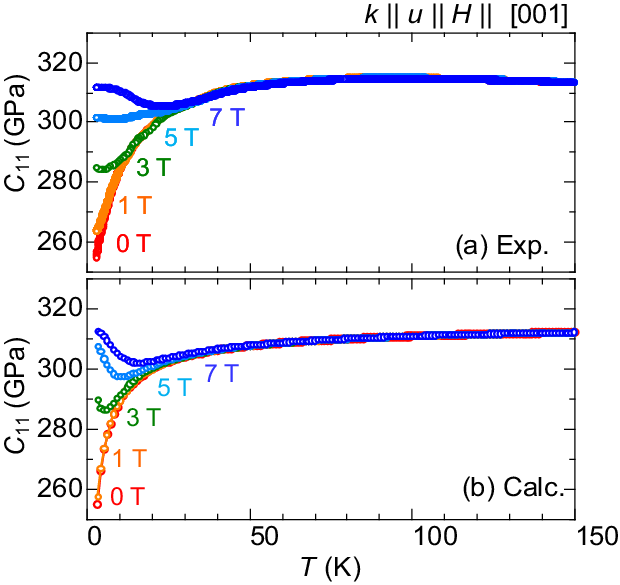
The first term is the background elastic constant corresponding to the contribution from the purely elastic energy, and the second term is the modification by the quadrupole-strain coupling. For simplicity, is approximated to be constant and temperature independent. The represents the statistical average of the quadrupole moment defined as . Here are -th eigenstates. The derivative term was approximated to , where was set to small finite value of the order of . The and means with and without the small . Figure A2 shows comparison of experimental and calculated as a function of temperature. Our calculation reproduces the overall behavior including a broad dip at above 3 T. This supports our calculation and estimated parameters are reasonable.
B.4 Magnetostriction
By minimizing the free energy with respect to the strain tensors Pukhov et al. 1985; Klekovkina et al. 2011 (i.e., ), one gets coupled equations as follows:
Then, three strain tensors can be given by
where
Figure A1(d) shows the magnetic field induced evolution of electric quadrupolar moments at = 2. Here and represents the lowest CEF level at each magnetic field. Trigonal crystalline field inherent in the pyrochlore systems induces moment even at zero field. The confirmed magnetostriction can be attributable to the magnetically-induced local quadrupolar moments of , and .
The best fitting parameters used in the present calculation are = 315 GPa, = 175 GPa, = 80 K and = 150 K. The signs of and are determined from longitudinal and transverse magnetostrictions. cannot be determined since it does not contribute , and .
References
- Anderson (1987) P. W. Anderson, Science 235, 1196 (1987).
- Balents (2010) L. Balents, Nature 464, 199 (2010).
- Ramirez et al. (1999) A. P. Ramirez, A. Hayashi, R. J. Cava, R. Siddharthan, and B. Shastry, Nature 399, 333 (1999).
- Castelnovo et al. (2008) C. Castelnovo, R. Moessner, and S. L. Sondhi, Nature 451, 42 (2008).
- Lee et al. (2012) S. Lee, S. Onoda, and L. Balents, Phys. Rev. B 86, 104412 (2012).
- Onoda and Tanaka (2011) S. Onoda and Y. Tanaka, Phys. Rev. B 83, 094411 (2011).
- Savary and Balents (2012) L. Savary and L. Balents, Phys. Rev. Lett. 108, 037202 (2012).
- Gardner et al. (2010) J. S. Gardner, M. J. Gingras, and J. E. Greedan, Rev. Mod. Phys. 82, 53 (2010).
- Gingras and McClarty (2014) M. J. Gingras and P. A. McClarty, Rep. Prog. Phys. 77, 056501 (2014).
- Rau and Gingras (2019) J. G. Rau and M. J. Gingras, Annu. Rev. Condens. Matter Phys. 10, 357 (2019).
- Gingras et al. (2000) M. Gingras, B. Den Hertog, M. Faucher, J. Gardner, S. Dunsiger, L. Chang, B. Gaulin, N. Raju, and J. Greedan, Phys. Rev. B 62, 6496 (2000).
- Molavian et al. (2007) H. R. Molavian, M. J. Gingras, and B. Canals, Phys. Rev. Lett. 98, 157204 (2007).
- Gardner et al. (1999) J. Gardner, S. Dunsiger, B. Gaulin, M. Gingras, J. Greedan, R. Kiefl, M. Lumsden, W. MacFarlane, N. Raju, J. Sonier, et al., Phys. Rev. Lett. 82, 1012 (1999).
- Gardner et al. (2003) J. Gardner, A. Keren, G. Ehlers, C. Stock, E. Segal, J. Roper, B. Fåk, M. Stone, P. Hammar, D. Reich, et al., Phys. Rev. B 68, 180401 (2003).
- Dunsiger et al. (2003) S. Dunsiger, R. Kiefl, J. Chakhalian, K. Chow, J. Gardner, J. Greedan, W. MacFarlane, R. Miller, G. Morris, A. Price, et al., Physica B: Condens. Matter 326, 475 (2003).
- Hamaguchi et al. (2004) N. Hamaguchi, T. Matsushita, N. Wada, Y. Yasui, and M. Sato, Phys. Rev. B 69, 132413 (2004).
- Gardner et al. (2004) J. Gardner, G. Ehlers, S. Bramwell, and B. Gaulin, J. Phys. Condens. Matter 16, S643 (2004).
- Rule et al. (2006) K. Rule, J. Ruff, B. Gaulin, S. Dunsiger, J. Gardner, J. Clancy, M. Lewis, H. Dabkowska, I. Mirebeau, P. Manuel, et al., Phys. Rev. Lett. 96, 177201 (2006).
- Takatsu et al. (2016) H. Takatsu, S. Onoda, S. Kittaka, A. Kasahara, Y. Kono, T. Sakakibara, Y. Kato, B. Fåk, J. Ollivier, J. W. Lynn, T. Taniguchi, M. Wakita, and H. Kadowaki, Phys. Rev. Lett. 116, 217201 (2016).
- Gritsenko et al. (2020) Y. Gritsenko, S. Mombetsu, P. T. Cong, T. Stöter, E. L. Green, C. S. Mejia, J. Wosnitza, M. Ruminy, T. Fennell, A. A. Zvyagin, S. Zherlitsyn, and M. Kenzelmann, Phys. Rev. B 102, 060403 (2020).
- Lüthi (2007) B. Lüthi, Physical acoustics in the solid state, Vol. 148 (Springer Science & Business Media, 2007).
- Mamsurova et al. (1988) L. Mamsurova, K. Pigal’skij, K. Pukhov, N. Trusevich, and L. Shcherbakova, Zh. Eksp. Teor. Fiz 94, 209 (1988).
- Nakanishi et al. (2011) Y. Nakanishi, T. Kumagai, M. Yoshizawa, K. Matsuhira, S. Takagi, and Z. Hiroi, Phys. Rev. B 83, 184434 (2011).
- Pukhov et al. (1985) K. Pukhov, N. Trusevich, and L. Shcherbakova, Zh. Eksp. Teor. Fiz 89, 2230 (1985).
- Ruff et al. (2010) J. Ruff, Z. Islam, J. Clancy, K. Ross, H. Nojiri, Y. Matsuda, H. Dabkowska, A. Dabkowski, and B. Gaulin, Phys. Rev. Lett. 105, 077203 (2010).
- Li et al. (2013) Q. Li, Z. Zhao, C. Fan, F. Zhang, H. Zhou, X. Zhao, and X. Sun, Phys. Rev. B 87, 214408 (2013).
- Hirschberger et al. (2015) M. Hirschberger, R. Chisnell, Y. S. Lee, and N. P. Ong, Phys. Rev. Lett. 115, 106603 (2015).
- Hirokane et al. (2019) Y. Hirokane, Y. Nii, Y. Tomioka, and Y. Onose, Phys. Rev. B 99, 134419 (2019).
- Fennell et al. (2014) T. Fennell, M. Kenzelmann, B. Roessli, H. Mutka, J. Ollivier, M. Ruminy, U. Stuhr, O. Zaharko, L. Bovo, A. Cervellino, M. K. Haas, and R. J. Cava, Phys. Rev. Lett. 112, 017203 (2014).
- Ruminy et al. (2016a) M. Ruminy, L. Bovo, E. Pomjakushina, M. Haas, U. Stuhr, A. Cervellino, R. J. Cava, M. Kenzelmann, and T. Fennell, Phys. Rev. B 93, 144407 (2016a).
- Constable et al. (2017) E. Constable, R. Ballou, J. Robert, C. Decorse, J.-B. Brubach, P. Roy, E. Lhotel, L. Del-Rey, V. Simonet, S. Petit, et al., Phys. Rev. B 95, 020415 (2017).
- Klekovkina et al. (2011) V. Klekovkina, A. Zakirov, B. Malkin, and L. Kasatkina, in J. Phys. Conf. Ser., Vol. 324 (IOP Publishing, 2011) p. 012036.
- Wakita et al. (2016) M. Wakita, T. Taniguchi, H. Edamoto, H. Takatsu, and H. Kadowaki, J. Phys. Conf. Ser. 683, 012023 (2016).
- Taniguchi et al. (2013) T. Taniguchi, H. Kadowaki, H. Takatsu, B. Fåk, J. Ollivier, T. Yamazaki, T. J. Sato, H. Yoshizawa, Y. Shimura, T. Sakakibara, T. Hong, K. Goto, L. R. Yaraskavitch, and J. B. Kycia, Phys. Rev. B 87, 060408 (2013).
- Ruff et al. (2007) J. Ruff, B. Gaulin, J. Castellan, K. Rule, J. Clancy, J. Rodriguez, and H. Dabkowska, Phys. Rev. Lett. 99, 237202 (2007).
- Guitteny et al. (2013) S. Guitteny, J. Robert, P. Bonville, J. Ollivier, C. Decorse, P. Steffens, M. Boehm, H. Mutka, I. Mirebeau, and S. Petit, Phys. Rev. Lett. 111, 087201 (2013).
- Hallas et al. (2020) A. Hallas, W. Jin, J. Gaudet, E. Tonita, D. Pomaranski, C. Buhariwalla, M. Tachibana, N. Butch, S. Calder, M. Stone, et al., arXiv:2009.05036 (2020).
- Ruminy et al. (2016b) M. Ruminy, E. Pomjakushina, K. Iida, K. Kamazawa, D. Adroja, U. Stuhr, and T. Fennell, Phys. Rev. B 94, 024430 (2016b).
- Hutchings (1964) M. T. Hutchings, in Solid state physics, Vol. 16 (Elsevier, 1964) pp. 227–273.