跳到论文正文
W Papers独立论文阅读器 arXiv:2109.11795 论文正文 计算阅读时间 · 0%
引用这篇论文根据当前论文元数据生成,正式投稿前建议核对。


License: arXiv.org perpetual non-exclusive license
arXiv:2109.11795v1 [stat.ME] 24 Sep 2021

Scalable Bayesian high-dimensional local dependence learning

Kyoungjae Lee Affiliation: Department of Statistics, Sungkyunkwan university    Lizhen Lin Affiliation: Department of Applied and Computational Mathematics and Statistics, University of Notre Dame
Abstract

In this work, we propose a scalable Bayesian procedure for learning the local dependence structure in a high-dimensional model where the variables possess a natural ordering. The ordering of variables can be indexed by time, the vicinities of spatial locations, and so on, with the natural assumption that variables far apart tend to have weak correlations. Applications of such models abound in a variety of fields such as finance, genome associations analysis and spatial modeling. We adopt a flexible framework under which each variable is dependent on its neighbors or predecessors, and the neighborhood size can vary for each variable. It is of great interest to reveal this local dependence structure by estimating the covariance or precision matrix while yielding a consistent estimate of the varying neighborhood size for each variable. The existing literature on banded covariance matrix estimation, which assumes a fixed bandwidth cannot be adapted for this general setup. We employ the modified Cholesky decomposition for the precision matrix and design a flexible prior for this model through appropriate priors on the neighborhood sizes and Cholesky factors. The posterior contraction rates of the Cholesky factor are derived which are nearly or exactly minimax optimal, and our procedure leads to consistent estimates of the neighborhood size for all the variables. Another appealing feature of our procedure is its scalability to models with large numbers of variables due to efficient posterior inference without resorting to MCMC algorithms. Numerical comparisons are carried out with competitive methods, and applications are considered for some real datasets.

Keywords: Selection consistency, optimal posterior convergence rate, varying bandwidth.

1 Introduction

The problem of covariance matrix or precision matrix estimation has been extensively studied over the last few decades. A typical model setup is to assume X=(X1,…,Xp)T∈ℝpX=(X_{1},\ldots,X_{p})^{T}\in\mathbb{R}^{p} follows a pp-dimensional normal distribution Np​(0,Σ)N_{p}(0,\Sigma), with mean zero and covariance matrix Σ∈ℝp×p\Sigma\in\mathbb{R}^{p\times p}. The dependence structure among the variables is encoded by the covariance matrix Σ\Sigma or its inverse Ω=Σ−1\Omega=\Sigma^{-1}. In high-dimensional settings where pp can be much larger than the sample size, the traditional sample covariance matrix or inverse-Wishart prior leads to inconsistent estimates of Σ\Sigma or Ω\Omega, see Johnstone and Lu 2009 and Lee and Lee 2018. Restricted matrix classes with a banded or sparse structure are often imposed on the covariance or precision matrices as a common practice for consistent estimation (see, e.g., Bickel and Levina 2008, Cai et al. 2016 and Lee et al. 2019).

In this paper, we focus on investigating the local dependence structure in a high-dimension model where the variables possess a natural ordering. An ordering on variables is often encountered for example in time series or genome data, where variables close to each other in time or location are more likely to be correlated than variables located far apart. More specifically, we assume that each variable depends on its neighboring variables or predecessors  and more importantly, the the size of the neighborhood or bandwidth can vary with each variable. Therefore, the existing literature on banded covariance matrix estimation which deals with a fixed bandwidth cannot be adapted for this set up.

Our work employs the modified Cholesky decomposition (MCD) (Pourahmadi 1999) of the precision matrix, which provides an efficient way to learn the local dependence structure of the data. The MCD has been widely used for covariance or precision matrix estimation including in Rütimann and Bühlmann 2009, Shojaie and Michailidis 2010 and van de Geer and Bühlmann 2013, just to name a few.  In more details, assume the variables X1,…,XpX_{1},\ldots,X_{p} are  arranged according to a known ordering. For any p×pp\times p positive definite matrix Ω\Omega, there uniquely exist lower triangular matrix A=(aj​l)∈ℝp×pA=(a_{jl})\in\mathbb{R}^{p\times p} and diagonal matrix D=d​i​a​g​(dj)∈ℝp×pD=diag(d_{j})\in\mathbb{R}^{p\times p}  such that Ω=(Ip−A)T​D−1​(Ip−A)\Omega=(I_{p}-A)^{T}D^{-1}(I_{p}-A), where aj​j=0a_{jj}=0 and dj>0d_{j}>0 for all j=1,…,pj=1,\ldots,p. It is called the MCD of Ω\Omega, and we call AA the Cholesky factor. Based on the MCD, X=(X1,…,Xp)T∼Np​(0,Ω−1)X=(X_{1},\ldots,X_{p})^{T}\sim N_{p}(0,\Omega^{-1}) is equivalent to a set of linear regression models, X1∼N⁡(0,d1)X_{1}\sim N(0,d_{1}) and

Xj|X1,…,Xj−1\displaystyle X_{j}\mid X_{1},\ldots,X_{j-1} ∼\displaystyle\sim N⁡(∑l=1j−1aj​l​Xl,dj),j=2,…,p.\displaystyle N\Big(\sum_{l=1}^{j-1}a_{jl}X_{l},\,\,d_{j}\Big),\quad j=2,\ldots,p. (1)

In this paper, we assume local dependence structure by considering

Xj|Xj−kj,…,Xj−1\displaystyle X_{j}\mid X_{j-k_{j}},\ldots,X_{j-1} ∼\displaystyle\sim N⁡(∑l=j−kjj−1aj​l​Xl,dj),j=2,…,p\displaystyle N\Big(\sum_{l=j-k_{j}}^{j-1}a_{jl}X_{l},\,\,d_{j}\Big),\quad j=2,\ldots,p (2)

for some kjk_{j} instead of (1), which implies aj​l=0a_{jl}=0 for any l=1,…,j−kj−1l=1,\ldots,j-k_{j}-1 and j=2,…,pj=2,\ldots,p. It leads to a varying bandwidth structure for the Cholesky factor which means that XjX_{j} is dependent only on kjk_{j} closest variables, Xj−kj,…,Xj−1X_{j-k_{j}},\ldots,X_{j-1}, and conditionally independent of others. Our goal is to learn the local dependence structure of data based on model (2) by learning aj​l,dja_{jl},d_{j} as well as the varying bandwidth or neighborhood size kjk_{j}. Allowing a varying bandwidth in the above model is a more realistic assumption as the range and pattern of dependence can vary over time or spatial locations.  See Figure 1 for an illustration of the Cholesky structure with varying bandwidth.

A number of work have been proposed for estimating sparse Cholesky factors based on penalized likelihood approaches, including Rothman et al. 2010, van de Geer and Bühlmann 2013 and Khare et al. 2019. However, these methods are not suitable for modeling local dependence because they allow arbitrary sparsity patterns for Cholesky factors. For example, XjX_{j} can depend on X1X_{1} but not on X2,…,Xj−1X_{2},\ldots,X_{j-1} in their framework, which is not desirable in the context of local dependence. An et al. 2014 considered a banded Cholesky factor and proposed a consistent test for bandwidth selection, but they assumed the same local dependence structure for all variables, that is, assumed a common kk instead of kjk_{j} in (2). The most relevant work is Yu and Bien 2017 which developed a penalized likelihood approach for estimating the banded Cholesky factor in (2) using a hierarchical group lasso penalty. Their approach is formulated as a convex optimization problem, and theoretical properties such as selection consistency and convergence rates were established. However, they required relatively strong conditions to obtain theoretical results, which will be discussed in detail in Section 3.

From a Bayesian perspective, Banerjee and Ghosal 2014 and Lee and Lee 2021 suggested GG-Wishart priors and banded Cholesky priors for learning local dependence structure with a common bandwidth kk, and posterior convergence rates for precision matrices are derived assuming kk is known. Lee et al. 2019 proposed the empirical sparse Cholesky prior for sparse Cholesky factors. Under their model each variable can be dependent on distant variables, so it is not suitable for local dependence structure. Lee and Lin 2020 suggested a prior distribution for banded Cholesky factors. Although bandwidth selection consistency as well as consistency of Bayes factors were established in high-dimensional settings, again a common bandwidth kk is assumed in their model. Achieving selection consistency simultaneously for bandwidths of all the variables is a much more challenging problem as the number of bandwidths as well as the size of the bandwidth can diverge as the number of variables pp goes to infinity.

In this paper, we propose a prior tailored to Cholesky factors with local dependence structure. The proposed prior allows a flexible learning of local dependence structure based on varying bandwidth kjk_{j}. This paper contributes in both theoretical and practical developments. For theoretical advancement, we prove selection consistency for varying bandwidth and nearly  optimal posterior convergence rates for Cholesky factors. This is the first Bayesian method for local dependence learning with varying bandwidth in high-dimensional settings with theoretical guarantees. Furthermore, we significantly weaken required conditions to obtain theoretical properties compared with those in Yu and Bien 2017. On the other hand, from a practical point of view, the induced posterior allows fast computations, enabling scalable inference for large data sets.  The posterior inference does not require Markov chain Monte Carlo (MCMC) algorithms and is easily parallelizable. Furthermore, our simulation studies show that the proposed method outperforms other competitors in various settings. We find that the proposed cross-validation for the proposed method is much faster than the contenders and selects nearly optimal hyperparameter in terms of specificity and sensitivity. Finally, it is worth mentioning that posterior inference for sparse Cholesky factors with an arbitrary sparsity pattern is computationally much more expensive than that for banded Cholesky factors, developing a statistical method for banded Cholesky factors is therefore of great importance independent of existing methods for sparse Cholesky factors.

The rest of paper is organized as follows. In Section 2, model assumptions, the proposed local dependence Cholesky prior and the induced fractional posterior are introduced. The main results including bandwidth selection consistency and optimal posterior convergence rates are established in Section 3. In Section 4, the performance of the proposed method is illustrated based on simulated data and real data analysis. Concluding remarks and discussions are given in Section 5, while the proofs of main results and additional simulation results are provided in the Appendix. R codes for implementation of our empirical results are available at https://github.com/leekjstat/LANCE.

2 Preliminaries

2.1 Notation

For any aa and b∈ℝb\in\mathbb{R}, we denote a∧ba\wedge b and a∨ba\vee b as the minimum and maximum of aa and bb, respectively. For any positive sequences ana_{n} and bnb_{n}, an=o⁡(bn)a_{n}=o(b_{n}) denotes an/bn⟶0a_{n}/b_{n}\longrightarrow 0 as n→∞n\to\infty. We denote an=O⁡(bn)a_{n}=O(b_{n}), or equivalently an≲bna_{n}\lesssim b_{n}, if there exists a constant C>0C>0 such that an<C​bna_{n}<Cb_{n} for all large nn. For any matrix A=(ai​j)∈ℝp×pA=(a_{ij})\in\mathbb{R}^{p\times p}, we denote λmin​(A)\lambda_{\min}(A) and λmax​(A)\lambda_{\max}(A) as the minimum and maximum eigenvalues, respectively. Furthermore, we define the matrix ℓ∞\ell_{\infty}-norm, Frobenius norm and element-wise maximum norm as follows: ‖A‖∞=max⁡∑j=1p1≤i≤p⁡|ai​j|\|A\|_{\infty}=\max_{1\leq i\leq p}\sum_{j=1}^{p}|a_{ij}|, ‖A‖F=(∑i=1p∑j=1pai​j2)1/2\|A\|_{F}=(\sum_{i=1}^{p}\sum_{j=1}^{p}a_{ij}^{2})^{1/2} and ‖A‖max=max1≤i,j≤p⁡|ai​j|\|A\|_{\max}=\max_{1\leq i,j\leq p}|a_{ij}|.  We denote I​G​(a,b)IG(a,b) as the inverse-Gamma distribution with shape parameter a>0a>0 and scale parameter b>0b>0.

2.2 High-dimensional Gaussian Models

Throughout the paper, we assume a high-dimensional setting with p=pn≥np=p_{n}\geq n, and that the variables have a known natural ordering. Specifically, we assume we observe a sample of data with sample size nn from a pp-dimensional Gaussian model,

X1,…,Xn|Ωn\displaystyle X_{1},\ldots,X_{n}\mid\Omega_{n} ∼i.i.d.\displaystyle\overset{i.i.d.}{\sim} Np​(0,Ωn−1),\displaystyle N_{p}(0,\Omega_{n}^{-1}), (3)

where Ωn=Σn−1∈ℝp×p\Omega_{n}=\Sigma_{n}^{-1}\in\mathbb{R}^{p\times p} is a precision matrix. For the rest of the paper, we use subscript nn for any p×pp\times p matrices to indicate that the dimension p=pnp=p_{n} grows as n→∞n\to\infty. Let 𝐗n=(X1,…,Xn)T∈ℝn×p{\bf X}_{n}=(X_{1},\ldots,X_{n})^{T}\in\mathbb{R}^{n\times p} be a data matrix, and Xi=(Xi​1,…,Xi​p)T∈ℝpX_{i}=(X_{i1},\ldots,X_{ip})^{T}\in\mathbb{R}^{p} for all i=1,…,ni=1,\ldots,n. We denote the Cholesky factor and the diagonal matrix from the MCD as AnA_{n} and DnD_{n}, respectively, i.e., Ωn=(Ip−An)T​Dn−1​(Ip−An)\Omega_{n}=(I_{p}-A_{n})^{T}D_{n}^{-1}(I_{p}-A_{n}). Model (3) is related to a directed acyclic graph (DAG) model depending on the sparsity pattern of AnA_{n} (van de Geer and Bühlmann 2013; Lee et al. 2019), but we will not go into detail on DAG models.

In this paper, we assume An=(aj​l)A_{n}=(a_{jl}) has a banded structure with varying bandwidths, {k2,…,kp}\{k_{2},\ldots,k_{p}\}, which satisfies 0≤kj≤j−10\leq k_{j}\leq j-1 and ∑l:|j−l|>kj|aj​l|=0\sum_{l:|j-l|>k_{j}}|a_{jl}|=0 for each j=2,…,pj=2,\ldots,p. Let X~j∈ℝn\tilde{X}_{j}\in\mathbb{R}^{n} and 𝐗j⁡(kj)∈ℝn×kj{\bf X}_{j(k_{j})}\in\mathbb{R}^{n\times k_{j}} be sub-matrices of 𝐗n{\bf X}_{n} consisting of the jjth and (j−kj),…,(j−1)(j-k_{j}),\ldots,(j-1)th columns, respectively. Under the varying bandwidths assumption, model (3) can be represented as

X~1|d1\displaystyle\tilde{X}_{1}\mid d_{1} ∼\displaystyle\sim Nn​(0,d1​In),\displaystyle N_{n}(0,d_{1}I_{n}),
X~j|𝐗j⁡(kj),aj(kj),dj,kj\displaystyle\tilde{X}_{j}\mid{\bf X}_{j(k_{j})},a_{j}^{(k_{j})},d_{j},k_{j} ∼\displaystyle\sim Nn​(𝐗j⁡(kj)​aj(kj),dj​In),j=2,…,p,\displaystyle N_{n}\big({\bf X}_{j(k_{j})}a_{j}^{(k_{j})},d_{j}I_{n}\big),\quad j=2,\ldots,p,

where aj(kj)=(aj​l)(j−kj)≤l≤(j−1)∈ℝkja_{j}^{(k_{j})}=(a_{jl})_{(j-k_{j})\leq l\leq(j-1)}\in\mathbb{R}^{k_{j}}. The above representation implies that to predict the jjth variable, X~j\tilde{X}_{j}, it suffices to know its kjk_{j}-nearest predecessors, 𝐗j⁡(kj){\bf X}_{j(k_{j})}. Thus, the varying bandwidths assumption of AnA_{n} directly induces the local dependence structure between variables. As mentioned before, this is often natural given commonly encountered ordered variables in time series or genome data sets, and a more realistic and flexible assumption than the common bandwidth assumption.

2.3 Local Dependence Cholesky Prior

To conduct Bayesian inference, we need to impose a prior on AnA_{n} and DnD_{n} as well as kjk_{j}, j=2,…,pj=2,\ldots,p, which restricts AnA_{n} to have a local dependence structure. We propose the following prior

aj(kj)|dj,kj∼i​n​d.​Nkj​(a^j(kj),djγ​(𝐗j⁡(kj)T​𝐗j⁡(kj))−1),j=2,…,p,π⁡(dj)∝dj−ν0/2−1,j=1,…,p,π⁡(kj)∝c1−kjp−c2​kjI(0≤kj≤{Rj∧(j−1)}),j=2,…,p,\displaystyle\begin{split}a_{j}^{(k_{j})}\mid d_{j},k_{j}\,\,&\overset{ind.}{\sim}\,\,N_{k_{j}}\Big(\widehat{a}_{j}^{(k_{j})},\frac{d_{j}}{\gamma}\big({\bf X}_{j(k_{j})}^{T}{\bf X}_{j(k_{j})}\big)^{-1}\Big),\,\,j=2,\ldots,p,\\ \pi(d_{j})\,\,&\propto\,\,d_{j}^{-\nu_{0}/2-1},\,\,j=1,\ldots,p,\\ \pi(k_{j})\,\,&\propto\,\,c_{1}^{-k_{j}}p^{-c_{2}k_{j}}I(0\leq k_{j}\leq\{R_{j}\wedge(j-1)\}),\,\,j=2,\ldots,p,\end{split} (4)

for some positive constants γ,c1,c2,R2,…,Rp\gamma,c_{1},c_{2},R_{2},\ldots,R_{p} and ν0\nu_{0}, where a^j(kj)=(𝐗j⁡(kj)T​𝐗j⁡(kj))−1​𝐗j⁡(kj)T​X~j\widehat{a}_{j}^{(k_{j})}=({\bf X}_{j(k_{j})}^{T}{\bf X}_{j(k_{j})})^{-1}{\bf X}_{j(k_{j})}^{T}\tilde{X}_{j}. We call the above prior LANCE (LocAl depeNdence CholEsky) prior. The conditional prior for aj(kj)a_{j}^{(k_{j})} is a version of the Zellner’s g-prior (Zellner 1986) and depends on the data. By using the prior π⁡(aj(kj)∣dj,kj)\pi(a_{j}^{(k_{j})}\mid d_{j},k_{j}) with sub-Gaussian tails and data-dependent center, we can obtain theoretical properties of posteriors without having to use priors with heavier tails or introducing redundant upper bound conditions on ‖aj(kj)‖2\|a_{j}^{(k_{j})}\|_{2} as discussed by Lee et al. 2019. The prior for djd_{j} is improper and includes the Jeffreys’ prior (Jeffreys 1946), π⁡(dj)∝dj−1\pi(d_{j})\propto d_{j}^{-1}, as a special case. In fact, the proper prior dj∼I​G​(ν0/2,ν0′)d_{j}\sim IG(\nu_{0}/2,\nu_{0}^{\prime}), for some constant ν0′>0\nu_{0}^{\prime}>0, can be used. However, we proceed with the above improper prior to reduce the number of hyperparameters.

For posterior inference, we suggest using the fractional posterior, which has received increased attention recently (Martin and Walker 2014; Martin et al. 2017; Lee et al. 2019). Let L⁡(An,Dn)L(A_{n},D_{n}) be the likelihood function of model (3). For a given constant 0<α<10<\alpha<1, the α\alpha-fractional posterior is defined by πα​(An,Dn∣𝐗n)∝L​(An,Dn)α​π​(An,Dn)\pi_{\alpha}(A_{n},D_{n}\mid{\bf X}_{n})\propto L(A_{n},D_{n})^{\alpha}\pi(A_{n},D_{n}). Thus, α\alpha-fractional posterior is a posterior distribution updated with the likelihood function raised to a power of α\alpha instead of the usual likelihood. We denote the α\alpha-fractional posterior by πα(⋅∣𝐗n)\pi_{\alpha}(\cdot\mid{\bf X}_{n}) to indicate the use of α\alpha-fractional likelihood. Theoretical properties of fractional posterior can often be established under weaker conditions compared with the usual posterior (Bhattacharya et al. 2019). Under our model, the α\alpha-fractional posterior has the following closed form:

aj(kj)|dj,kj,𝐗n∼i​n​d.​Nkj​(a^j(kj),djα+γ​(𝐗j⁡(kj)T​𝐗j⁡(kj))−1),j=2,…,p,dj|kj,𝐗n∼i​n​d.​I​G​(α​n+ν02,α​n2​d^j(kj)),j=1,…,p,πα​(kj∣𝐗n)∝π(kj)(1+αγ)−kj2(d^j(kj))−α​n+ν02,j=2,…,p,\displaystyle\begin{split}a_{j}^{(k_{j})}\mid d_{j},k_{j},{\bf X}_{n}\,\,&\overset{ind.}{\sim}\,\,N_{k_{j}}\Big(\widehat{a}_{j}^{(k_{j})},\frac{d_{j}}{\alpha+\gamma}\big({\bf X}_{j(k_{j})}^{T}{\bf X}_{j(k_{j})}\big)^{-1}\Big),\,\,j=2,\ldots,p,\\ d_{j}\mid k_{j},{\bf X}_{n}\,\,&\overset{ind.}{\sim}\,\,IG\Big(\frac{\alpha n+\nu_{0}}{2},\,\frac{\alpha n}{2}\widehat{d}_{j}^{(k_{j})}\Big),\,\,j=1,\ldots,p,\\ \pi_{\alpha}(k_{j}\mid{\bf X}_{n})\,\,&\propto\,\,\pi(k_{j})\Big(1+\frac{\alpha}{\gamma}\Big)^{-\frac{k_{j}}{2}}\big(\widehat{d}_{j}^{(k_{j})}\big)^{-\frac{\alpha n+\nu_{0}}{2}},\,\,j=2,\ldots,p,\end{split} (5)

where d^j(kj)=n−1​X~jT​(In−P~j​kj)​X~j\widehat{d}_{j}^{(k_{j})}=n^{-1}\tilde{X}_{j}^{T}(I_{n}-\tilde{P}_{jk_{j}})\tilde{X}_{j} and P~j​kj=𝐗j⁡(kj)​(𝐗j⁡(kj)T​𝐗j⁡(kj))−1​𝐗j⁡(kj)T\tilde{P}_{jk_{j}}={\bf X}_{j(k_{j})}({\bf X}_{j(k_{j})}^{T}{\bf X}_{j(k_{j})})^{-1}{\bf X}_{j(k_{j})}^{T}. Based on (5), one can notice that posterior inference for each j=2,…,pj=2,\ldots,p is parallelizable. Furthermore, a MCMC algorithm is not needed because direct posterior sampling from (5) is possible. Note that the three posterior distributions in (5) form the joint posterior distributions of (aj(kj),dj,kj)(a_{j}^{(k_{j})},d_{j},k_{j}), which are independent for each j=1,…,pj=1,\ldots,p. Thus, LANCE prior leads to a fast and scalable posterior inference even in high-dimensions.

3 Main Results

In this section, we show that LANCE prior accurately unravels the local dependence structure. More specifically, it is proved that LANCE prior attains bandwidth selection consistency for all bandwidths and nearly minimax posterior convergence rates for Cholesky factors. To obtain desired asymptotic properties of posteriors, we assume the following conditions:

  • (A1)

    λmax​(Ω0​n)​log⁡p/λmin​(Ω0​n)=o⁡(n)\lambda_{\max}(\Omega_{0n})\log p/\lambda_{\min}(\Omega_{0n})=o(n).

  • (A2)

    For some constant Mbm>c2+1M_{\rm bm}>c_{2}+1,

    min(j,l):a0,j​l≠0a0,j​l2d0​j\displaystyle\min_{(j,l):a_{0,jl}\neq 0}\frac{a_{0,jl}^{2}}{d_{0j}} ≥\displaystyle\geq 10​Mbm​λmax​(Ω0​n)(α+ν0/n)​(1−α−ν0/n)​log⁡pn.\displaystyle\frac{10M_{\rm bm}\,\,\lambda_{\max}(\Omega_{0n})}{(\alpha+\nu_{0}/n)(1-\alpha-\nu_{0}/n)}\frac{\log p}{n}.
  • (A3)

    k0​j≤Rjk_{0j}\leq R_{j} for any j=2,…,pj=2,\ldots,p, maxj⁡Rj​log​p≤n⁡(1+5​ϵ)/{Cbm​(1−2​ϵ)2}\max_{j}R_{j}\log p\leq n(1+5\sqrt{\epsilon})/\{C_{\rm bm}(1-2\epsilon)^{2}\}, where ϵ={(1−α)/10}2\epsilon=\{(1-\alpha)/10\}^{2} and Cbm=10​Mbm/{(α+ν0/n)​(1−α−ν0/n)}C_{\rm bm}=10M_{\rm bm}/\{(\alpha+\nu_{0}/n)(1-\alpha-\nu_{0}/n)\}

  • (A4)

    The hyperparameters satisfy ν0=O⁡(1)\nu_{0}=O(1), γ=O⁡(1)\gamma=O(1), c1=O⁡(1)c_{1}=O(1), c2>1c_{2}>1 and 0.6≤α<10.6\leq\alpha<1.

Condition (A1) allows the condition number λmax​(Ω0​n)/λmin​(Ω0​n)\lambda_{\max}(\Omega_{0n})/\lambda_{\min}(\Omega_{0n}) to grow to infinity at a rate slower than n/log⁡pn/\log p. This condition is weaker than the bounded eigenvalue conditions  used in Banerjee and Ghosal 2015, Khare et al. 2019 and Lee et al. 2019, which assume c<λmin​(Ω0​n)≤λmax​(Ω0​n)<Cc<\lambda_{\min}(\Omega_{0n})\leq\lambda_{\max}(\Omega_{0n})<C for some constants cc and C>0C>0. We note here that we require the bounded eigenvalue conditions for the (nearly) minimaxity of the posterior convergence rates in Theorems 3.2 and 3.3.

Condition (A2) determines the lower bound for the nonzero signals, a0,j​l2/d0​ja_{0,jl}^{2}/d_{0j}. This is called the beta-min condition. It has been well known that the beta-min condition is essential for variable selection (Bühlmann and van de Geer 2011; Martin et al. 2017) and support recovery for sparse matrices (Yu and Bien 2017; Cao et al. 2019). Condition (A2) implies that the rate of nonzero a0,j​l2/d0​ja_{0,jl}^{2}/d_{0j} should, at least, be λmax​(Ω0​n)​log⁡p/n\lambda_{\max}(\Omega_{0n})\log p/n, which has the same rate with log⁡p/n\log p/n under the bounded eigenvalue condition.

Condition (A3), together with condition (A4), provides an upper bound for the true bandwidth k0​jk_{0j}: they allow the maximum bandwidth, maxj⁡k0​j\max_{j}k_{0j}, to grow to infinity at a rate not faster than n/log⁡pn/\log p. The rest of condition (A4) presents sufficient conditions for hyperparameters to obtain theoretical properties. The conditions on c1c_{1} and c2c_{2} control the strength of penalty for large models, i.e., large bandwidths. Note that condition c2>1c_{2}>1 is weaker than the condition c2≥2c_{2}\geq 2 used in Lee et al. 2019, which implies that the local dependence assumption requires a weaker penalty compared with arbitrary sparsity patterns. In Section 4, we will give a practical guidance for the choice of hyperparameters.

Theorem 3.1 (Bandwidth selection consistency)

Consider model (3) and LANCE prior (4). Under conditions (A1)–(A4), we have

𝔼0​{πα​(kj≠k0​j​ for at least one ​2≤j≤p∣𝐗n)}\displaystyle\mathbb{E}_{0}\Big\{\pi_{\alpha}\big(k_{j}\neq k_{0j}\text{ for at least one }2\leq j\leq p\mid{\bf X}_{n}\big)\Big\} ⟶\displaystyle\longrightarrow 0 as ​n→∞.\displaystyle 0\quad\text{ as }n\to\infty.

Theorem 3.1 says that the posterior probability of incorrectly estimating local dependence structure, i.e., bandwidths, converges to zero in probability as n→∞n\to\infty. Thus, the proposed method can consistently recover local dependence structure for each variable.

We compare the above result with existing theoretical results in other work. First of all, we note here that Khare et al. 2019, Cao et al. 2019 and Lee et al. 2019 assumed arbitrary dependence structures for Cholesky factors, thus their methods are not tailored to local dependence structure considered in this paper. Although Bickel and Levina 2008, Banerjee and Ghosal 2014 and Lee and Lee 2021 focused on banded Cholesky factors, which result in banded precision matrices, they assumed a common dependence structure, i.e., a common bandwidth, for each variable, and did not provide bandwidth selection consistency.

To the best of our knowledge, the state-of-the-art theoretical result for estimating local dependence structure is obtained by Yu and Bien 2017. They proposed a penalized likelihood approach and obtained bandwidth selection consistency in a high-dimensional setting. They assumed that the eigenvalues of Ω0​n\Omega_{0n} lie in [κ−2,κ2][\kappa^{-2},\kappa^{2}] and the beta-min condition,

min(j,l):a0,j​l≠0|a0,j​l|d0​j\displaystyle\min_{(j,l):a_{0,jl}\neq 0}\frac{|a_{0,jl}|}{\sqrt{d_{0j}}} ≥\displaystyle\geq 8​ρ−1​(4​maxj​‖Σ0​n,k0​j−1‖∞+5​κ2)​2​‖D0​n‖∞​log⁡pn,\displaystyle 8\rho^{-1}(4\max_{j}\|\Sigma_{0n,k_{0j}}^{-1}\|_{\infty}+5\kappa^{2})\sqrt{2\|D_{0n}\|_{\infty}\frac{\log p}{n}},

for some constants κ>1\kappa>1 and ρ∈(0,1]\rho\in(0,1], where Σ0​n,k0​j=(σ0,i​l)j−k0​j≤i,l≤j\Sigma_{0n,k_{0j}}=(\sigma_{0,il})_{j-k_{0j}\leq i,l\leq j} denotes the sub-matrix of the true covariance matrix. Note that these conditions are more restrictive than our conditions (A1) and (A2). For example, ‖Σ0​n,k0​j−1‖∞=O⁡(k0​j1/2)\|\Sigma_{0n,k_{0j}}^{-1}\|_{\infty}=O(k_{0j}^{1/2}) holds under the bounded eigenvalue condition, so the beta-min condition in Yu and Bien 2017 implies that the minimum nonzero a0,j​l2/d0​ja_{0,jl}^{2}/d_{0j} is bounded below by maxj⁡k0​j​log​p/n\max_{j}k_{0j}\log p/n with respect to a constant multiple; in contrast, the rate of the lower bound in condition (A2) is log⁡p/n\log p/n under the bounded eigenvalue condition. Furthermore, they assumed the so-called irrepresentable condition,

max2≤j≤p⁡max1≤l≤j−k0​j−1​‖(Σ0​n)l,k0​j​Σ0​n,k0​j−1‖1≤6​(1−ρ)π2,\max_{2\leq j\leq p}\max_{1\leq l\leq j-k_{0j}-1}\|(\Sigma_{0n})_{l,k_{0j}}\Sigma_{0n,k_{0j}}^{-1}\|_{1}\leq\frac{6(1-\rho)}{\pi^{2}},

which is typically required for the lasso type methods with a random design matrix (e.g., see Wainwright 2009 and Khare et al. 2019). Yu and Bien 2017 proved the exact signed support recovery property under the above conditions and n>ρ−2​‖D0​n‖∞​κ2n>\rho^{-2}\|D_{0n}\|_{\infty}\kappa^{2} (12​π2​maxj​k0​j+32)​log⁡p(12\pi^{2}\max_{j}k_{0j}+32)\log p. Note that condition (A3) together with (A4) implies n>C​maxj⁡k0​j​log​pn>C\max_{j}k_{0j}\log p for some constant C>0C>0. Hence, stronger conditions are also required by Yu and Bien 2017 to establish bandwidth selection consistency compared with Theorem 3.1.

Next, we show that LANCE prior achieves nearly minimax posterior convergence rates for Cholesky factors. The posterior convergence rates are obtained with or without beta-min condition (A2). Under the beta-min condition, Theorem 3.2 presents posterior convergence rates based on various matrix norms.

Theorem 3.2 (Posterior convergence rates with beta-min condition)

Suppose that the conditions in Theorem 3.1 hold. If k0​log⁡p=o⁡(n)k_{0}\log p=o(n), where k0=maxj⁡k0​jk_{0}=\max_{j}k_{0j}, we have

𝔼0​[πα​{‖An−A0​n‖max≥Kchol​λmax​(Ω0​n)2λmin​(Ω0​n)2​(k0+log⁡pn)1/2∣𝐗n}]\displaystyle\mathbb{E}_{0}\Big[\pi_{\alpha}\Big\{\|A_{n}-A_{0n}\|_{\max}\geq K_{\rm chol}\frac{\lambda_{\max}(\Omega_{0n})^{2}}{\lambda_{\min}(\Omega_{0n})^{2}}\Big(\frac{k_{0}+\log p}{n}\Big)^{1/2}\mid{\bf X}_{n}\Big\}\Big] =\displaystyle= o⁡(1),\displaystyle o(1),
𝔼0​[πα​{‖An−A0​n‖∞≥Kchol​λmax​(Ω0​n)2λmin​(Ω0​n)2​k0​(k0+log⁡pn)1/2∣𝐗n}]\displaystyle\mathbb{E}_{0}\Big[\pi_{\alpha}\Big\{\|A_{n}-A_{0n}\|_{\infty}\geq K_{\rm chol}\frac{\lambda_{\max}(\Omega_{0n})^{2}}{\lambda_{\min}(\Omega_{0n})^{2}}\sqrt{k_{0}}\Big(\frac{k_{0}+\log p}{n}\Big)^{1/2}\mid{\bf X}_{n}\Big\}\Big] =\displaystyle= o⁡(1),\displaystyle o(1),
𝔼0​[πα​{‖An−A0​n‖F2≥Kchol​λmax​(Ω0​n)2λmin​(Ω0​n)2​∑j=2p(k0​j+log⁡j)n∣𝐗n}]\displaystyle\mathbb{E}_{0}\Big[\pi_{\alpha}\Big\{\|A_{n}-A_{0n}\|_{F}^{2}\geq K_{\rm chol}\frac{\lambda_{\max}(\Omega_{0n})^{2}}{\lambda_{\min}(\Omega_{0n})^{2}}\frac{\sum_{j=2}^{p}(k_{0j}+\log j)}{n}\mid{\bf X}_{n}\Big\}\Big] =\displaystyle= o⁡(1),\displaystyle o(1),

for some constant Kchol>0K_{\rm chol}>0 not depending on unknown parameters.

Estimating each row of Cholesky factor AnA_{n} can be considered as a linear regression problem with a random design matrix. By assuming beta-min condition (A2), we can use the selection consistency result in Theorem 3.1, although a beta-min condition is usually not essential for obtaining convergence rates. With a cost of the beta-min condition, we can focus only on the set aj(kj)=aj(k0​j)a_{j}^{(k_{j})}=a_{j}^{(k_{0j})} for all jj in the posterior with high probability tending to 1. Then the above posterior convergence rates for various matrix norms boil down to those related to ‖aj(k0​j)−a0​j(k0​j)‖\|a_{j}^{(k_{0j})}-a_{0j}^{(k_{0j})}\| for various vector norms ∥⋅∥\|\cdot\|, which makes the problem simpler.

Assume that ϵ0≤λmin​(Ω0​n)≤λmax​(Ω0​n)≤ϵ0−1\epsilon_{0}\leq\lambda_{\min}(\Omega_{0n})\leq\lambda_{\max}(\Omega_{0n})\leq\epsilon_{0}^{-1} for some small constant 0<ϵ0<1/20<\epsilon_{0}<1/2. Then, the obtained posterior convergence rates in Theorem 3.2 under the matrix ℓ∞\ell_{\infty}-norm and Frobenius norm are minimax if log⁡p=O⁡(k0)\log p=O(k_{0}) and log⁡j=O⁡(k0​j)\log j=O(k_{0j}) for all j=2,…,pj=2,\ldots,p, respectively, by Theorem 3.3 in Lee et al. 2019. Therefore, the above posterior convergence rates are nearly or exactly minimax depending on the dimensionality pp and bandwidths k0​jk_{0j} under bounded eigenvalue conditions on Ω0​n\Omega_{0n}.

Now, we establish posterior convergence rate of Cholesky factors without beta-min condition (A2). To obtain the desired result, we consider a modified LANCE prior using dj∼I​G​(ν0/2,ν0′)d_{j}\sim IG(\nu_{0}/2,\nu_{0}^{\prime}) for some constant ν0′>0\nu_{0}^{\prime}>0 instead of π(dj)∝dj−ν0/2−1\pi(d_{j})\propto d_{j}^{-\nu_{0}/2-1} in (4). This modification is mainly used to derive a lower bound of the likelihood ratio appearing in the denominator of posteriors (see Lemma 7.1 in Lee et al. 2019). Theorem 3.3 shows the posterior convergence rate under various matrix norms.

Theorem 3.3 (Posterior convergence rates without beta-min condition)

Consider model (3) and the modified LANCE prior described above. Suppose that the conditions (A1), (A3) and (A4) hold. If k0​log⁡p=o⁡(n)k_{0}\log p=o(n), λmax​(Ω0​n)/λmin​(Ω0​n)=O⁡(p)\lambda_{\max}(\Omega_{0n})/\lambda_{\min}(\Omega_{0n})=O(p) and λmax​(Ω0​n)=o⁡(n)\lambda_{\max}(\Omega_{0n})=o(n), we have

𝔼0​[πα​{‖An−A0​n‖max≥Kchol​(λmax​(Ω0​n)λmin​(Ω0​n)​k0​log⁡pn)1/2∣𝐗n}]\displaystyle\mathbb{E}_{0}\Big[\pi_{\alpha}\Big\{\|A_{n}-A_{0n}\|_{\max}\geq K_{\rm chol}\Big(\frac{\lambda_{\max}(\Omega_{0n})}{\lambda_{\min}(\Omega_{0n})}\frac{k_{0}\log p}{n}\Big)^{1/2}\mid{\bf X}_{n}\Big\}\Big] =\displaystyle= o⁡(1),\displaystyle o(1),
𝔼0​[πα​{‖An−A0​n‖∞≥Kchol​k0​(λmax​(Ω0​n)λmin​(Ω0​n)​log⁡pn)1/2∣𝐗n}]\displaystyle\mathbb{E}_{0}\Big[\pi_{\alpha}\Big\{\|A_{n}-A_{0n}\|_{\infty}\geq K_{\rm chol}{k_{0}}\Big(\frac{\lambda_{\max}(\Omega_{0n})}{\lambda_{\min}(\Omega_{0n})}\frac{\log p}{n}\Big)^{1/2}\mid{\bf X}_{n}\Big\}\Big] =\displaystyle= o⁡(1),\displaystyle o(1),
𝔼0​[πα​{‖An−A0​n‖F2≥Kchol​λmax​(Ω0​n)λmin​(Ω0​n)​∑j=2pk0​log⁡jn∣𝐗n}]\displaystyle\mathbb{E}_{0}\Big[\pi_{\alpha}\Big\{\|A_{n}-A_{0n}\|_{F}^{2}\geq K_{\rm chol}\frac{\lambda_{\max}(\Omega_{0n})}{\lambda_{\min}(\Omega_{0n})}\frac{\sum_{j=2}^{p}k_{0}\log j}{n}\mid{\bf X}_{n}\Big\}\Big] =\displaystyle= o⁡(1),\displaystyle o(1),

for some constant Kchol>0K_{\rm chol}>0 not depending on unknown parameters.

If we assume bounded eigenvalue conditions on Ω0​n\Omega_{0n}, the above posterior convergence rates are slightly slower than those in Theorem 3.2 due to the absence of the beta-min condition. Suppose ϵ0≤λmin​(Ω0​n)≤λmax​(Ω0​n)≤ϵ0−1\epsilon_{0}\leq\lambda_{\min}(\Omega_{0n})\leq\lambda_{\max}(\Omega_{0n})\leq\epsilon_{0}^{-1} for some small constant 0<ϵ0<1/20<\epsilon_{0}<1/2. Under these bounded eigenvalue conditions, Yu and Bien 2017 (Lemma 17) obtained the convergence rates ζΓ​log⁡p/n\zeta_{\Gamma}\sqrt{\log p/n}, ζΓ​(k0+1)​(log⁡p/n)1/2\zeta_{\Gamma}(k_{0}+1)(\log p/n)^{1/2} and ζΓ​(∑j=2pk0​j+p)​log⁡p/n\zeta_{\Gamma}\sqrt{(\sum_{j=2}^{p}k_{0j}+p)\log p/n} under the element-wise maximum norm, matrix ℓ∞\ell_{\infty}-norm and Frobenius norm, respectively, where ζΓ=8​(2​‖D0​n‖∞)1/2​ρ−1​(4​maxj​‖Σ0​n,k0​j−1‖∞+5​ϵ0−1)\zeta_{\Gamma}=8(2\|D_{0n}\|_{\infty})^{1/2}\rho^{-1}(4\max_{j}\|\Sigma_{0n,k_{0j}}^{-1}\|_{\infty}+5\epsilon_{0}^{-1}) for some constant ρ∈(0,1]\rho\in(0,1]. Note that, as mentioned before, it holds that ‖Σ0​n,k0​j−1‖∞=O⁡(k0​j1/2)\|\Sigma_{0n,k_{0j}}^{-1}\|_{\infty}=O(k_{0j}^{1/2}) without further assumption. Thus, their convergence rates are slower than or comparable to ours. We would also like to mention that, under bounded eigenvalue conditions on Ω0​n\Omega_{0n}, the posterior convergence rate under the matrix ℓ∞\ell_{\infty}-norm in Theorem 3.3 is minimax if log⁡p≍log⁡(p/k0)\log p\asymp\log(p/k_{0}) by Theorem 3.5 in Lee et al. 2019.  For example, it is the case if k0=O⁡(pβ)k_{0}=O(p^{\beta}) for some 0<β<10<\beta<1.

By carefully modifying the proof of Theorem 3.6 in Lee et al. 2019, we can probably obtain posterior convergence rates for precision matrices. However, it is not clear whether the obtained posterior convergence rates are minimax optimal. Although Liu and Ren 2020 showed minimax rates for precision matrices with bandable Cholesky factors, they considered slightly different parameter spaces for Cholesky factors from what we consider. To the best of our knowledge, minimax rates for precision matrices based on Cholesky factors with varying bandwidths have not been established.

4 Numerical Studies

4.1 Choice of hyperparameters

The proposed Bayesian method has hyperparameters that need to be determined, and we provide the following guidelines. It is reasonable to use the hyperparameter α\alpha close to 1 unless there is a strong evidence of model misspecification. Thus, in our numerical studies, α=0.99\alpha=0.99 is used. We use the hyperparameter ν0=0\nu_{0}=0, which leads to the Jeffreys’ prior (Jeffreys 1946) for djd_{j}. The upper bound for model sizes, RjR_{j}, is set at Rj=⌊n/2⌋−2R_{j}=\lfloor n/2\rfloor-2. The rest of hyperparameters γ,c1\gamma,c_{1} and c2c_{2} control the penalty for large models through πα​(kj∣𝐗n)\pi_{\alpha}(k_{j}\mid{\bf X}_{n}): as the values of γ,c1\gamma,c_{1} and c2c_{2} increase, πα​(kj∣𝐗n)\pi_{\alpha}(k_{j}\mid{\bf X}_{n}) prefers smaller values of kjk_{j}. We suggest to determine c2c_{2} using the Bayesian cross-validation method (Gelman et al. 2014), with the other hyperparameters γ=0.1\gamma=0.1 and c1=1c_{1}=1 fixed. Compared with the Bayesian cross-validation method for choosing (γ,c1,c2)(\gamma,c_{1},c_{2}), this approach significantly reduces computational time, while achieving nice performance in our simulation study.

To conduct Bayesian cross-validation, we repeatedly split the data ncvn_{\rm cv} times into a training set and a test set with size n1=⌈n/2⌉n_{1}=\lceil n/2\rceil and n2=⌊n/2⌋n_{2}=\lfloor n/2\rfloor, respectively. Let I1​(ν)I_{1}(\nu) and I2​(ν)I_{2}(\nu) be indices for the ν\nuth training set and test set, respectively, i.e., |I1​(ν)|=n1|I_{1}(\nu)|=n_{1}, |I2​(ν)|=n2|I_{2}(\nu)|=n_{2} and I1​(ν)∪I2​(ν)={1,…,n}I_{1}(\nu)\cup I_{2}(\nu)=\{1,\ldots,n\}, for any ν=1,…,ncv\nu=1,\ldots,n_{\rm cv}. Denote 𝐗I1​(ν){\bf X}_{I_{1}(\nu)} and 𝐗I2​(ν){\bf X}_{I_{2}(\nu)} as {Xi}i∈I1​(ν)\{X_{i}\}_{i\in I_{1}(\nu)} and {Xi}i∈I2​(ν)\{X_{i}\}_{i\in I_{2}(\nu)}, respectively. Then for a given hyperparameter c2c_{2}, the estimated out-of-sample log predictive density, lpdcv,c2\text{lpd}_{\rm cv,c_{2}}, is

lpdcv,c2\displaystyle\text{lpd}_{\rm cv,c_{2}} =\displaystyle= ∑ν=1ncvlog⁡fc2​(𝐗I2​(ν)∣𝐗I1​(ν))\displaystyle\sum_{\nu=1}^{n_{\rm cv}}\log f_{c_{2}}({\bf X}_{I_{2}(\nu)}\mid{\bf X}_{I_{1}(\nu)})
=\displaystyle= ∑ν=1ncvlog⁡{∑kf⁡(𝐗I2​(ν)∣k)​πα,c2​(k∣𝐗I1​(ν))},\displaystyle\sum_{\nu=1}^{n_{\rm cv}}\log\Big\{\sum_{k}f({\bf X}_{I_{2}(\nu)}\mid k)\pi_{\alpha,c_{2}}(k\mid{\bf X}_{I_{1}(\nu)})\Big\},

where k=(k2,…,kp)k=(k_{2},\ldots,k_{p}), f⁡(𝐗I2​(ν)∣k)f({\bf X}_{I_{2}(\nu)}\mid k) is the marginal likelihood for kk given 𝐗I2​(ν){\bf X}_{I_{2}(\nu)}, and πα,c2​(k∣𝐗I1​(ν))\pi_{\alpha,c_{2}}(k\mid{\bf X}_{I_{1}(\nu)}) is the fractional posterior based on 𝐗I1​(ν){\bf X}_{I_{1}(\nu)} and the hyperparameter c2c_{2}. The aim of the Bayesian cross-validation is to find the optimal c2c_{2} maximizing lpdcv,c2\text{lpd}_{\rm cv,c_{2}}.

The marginal likelihood f⁡(𝐗I2​(ν)∣k)f({\bf X}_{I_{2}(\nu)}\mid k) is available in a closed form:

f(𝐗I2​(ν)∣k)=∏j=2p[(2π)−n2/2Γ(n2+ν02)(1+1γ)−kj/2{d^j(kj)(I2(ν))/2}−(n2+ν0)/2],\displaystyle f({\bf X}_{I_{2}(\nu)}\mid k)\,=\,\prod_{j=2}^{p}\Bigg[(2\pi)^{-n_{2}/2}\Gamma\Big(\frac{n_{2}+\nu_{0}}{2}\Big)\Big(1+\frac{1}{\gamma}\Big)^{-k_{j}/2}\Big\{\widehat{d}_{j}^{(k_{j})}(I_{2}(\nu))/2\Big\}^{-(n_{2}+\nu_{0})/2}\Bigg],

where d^j(kj)​(I2​(ν))\widehat{d}_{j}^{(k_{j})}(I_{2}(\nu)) is the estimated variance d^j(kj)\widehat{d}_{j}^{(k_{j})} using 𝐗I2​(ν){\bf X}_{I_{2}(\nu)}. The closed form of the marginal posterior πα,c2​(kj∣𝐗I1​(ν))\pi_{\alpha,c_{2}}(k_{j}\mid{\bf X}_{I_{1}(\nu)}) is also available in (5), which requires the calculation of d^j(kj)​(I1​(ν))\widehat{d}_{j}^{(k_{j})}(I_{1}(\nu)). When calculating lpdcv,c2\text{lpd}_{\rm cv,c_{2}}, the main computational burden comes from calculating d^j(kj)​(I1​(ν))\widehat{d}_{j}^{(k_{j})}(I_{1}(\nu)) and d^j(kj)​(I2​(ν))\widehat{d}_{j}^{(k_{j})}(I_{2}(\nu)) for each kj=0,1,…,Rj∧(j−1)k_{j}=0,1,\ldots,R_{j}\wedge(j-1) and j=2,…,pj=2,\ldots,p. Note that these quantities do not vary from different choices of c2c_{2}. For a given randomly split data, these quantities only need to be calculated once regardless of the value of c2c_{2}. Therefore, LANCE prior enables scalable cross-validation-based inference even in high-dimensions. Throughout the numerical study, we split the data ncv=5n_{\rm cv}=5 times.

4.2 Simulated data

Throughout the numerical studies in this section, we focus on the bandwidth selection performance, while additional simulation studies focusing on the estimation performance are given in the Appendix.  We generated the true precision matrix Ω0​n=(Ip−A0​n)T​D0​n−1​(Ip−A0​n)\Omega_{0n}=(I_{p}-A_{0n})^{T}D_{0n}^{-1}(I_{p}-A_{0n}) for simulation studies. The diagonal entries of D0​n=d​i​a​g​(d0​j)D_{0n}=diag(d_{0j}) were drawn independently from U​n​i​f​(2,5)Unif(2,5). Next, the lower triangular entries of A0​n=(a0,j​l)A_{0n}=(a_{0,jl}) were generated as follows:

  • •

    Model 1: For 2≤v≤p2\leq v\leq p, the bandwidth of the vvth row of A0​nA_{0n} is sampled from U​n​i​f​{1,…,min⁡(v−1,5)}Unif\{1,\ldots,\min(v-1,5)\}. This produces a sparse Cholesky factor with the maximum bandwidth size 5.  Each nonzero element in A0​nA_{0n} is drawn independently from U​n​i​f​(A0,min,A0,max)Unif(A_{0,\min},A_{0,\max}), where the positive of negative sign is assigned with probability 0.5.

  • •

    Model 2: A0​nA_{0n} is a block diagonal matrix consisting of 5 blocks with size p/5p/5, while the maximum size of bandwidths is 40. This setting produces a moderately sparse Cholesky factor. The length of the bandwidth of the vvth row in each block follows a mixture distribution, 0.5×U​n​i​f​{1,…,min⁡(v−1,40)}+0.5×δ00.5\times Unif\{1,\ldots,\min(v-1,40)\}+0.5\times\delta_{0}, where δ0\delta_{0} is a point mass at zero. Each nonzero element in A0​nA_{0n} is drawn independently from U​n​i​f​(A0,min,A0,max)Unif(A_{0,\min},A_{0,\max}), where the positive or negative sign is assigned with probability 0.5. This setting corresponds to Model 2 in Yu and Bien 2017.

  • •

    Model 3: A0​nA_{0n} is a block diagonal matrix consisting of 2 blocks with size p/2p/2, and the rest of the generation process is similar to that of Model 2. This setting produces a denser Cholesky factor compared with Model 2. This setting corresponds to Model 3 in Yu and Bien 2017.

Figure 1 shows a simulated true Cholesky factors for Settings 1 and 2 with (A0,min,A0,max)=(0.1,0.4)(A_{0,\min},A_{0,\max})=(0.1,0.4) and p=100p=100.

Refer to caption
Figure 1: The true Cholesky factors for Model 1 (left), Model 2 (middle) and Model 3 (right) with (A0,min,A0,max)=(0.1,0.4)(A_{0,\min},A_{0,\max})=(0.1,0.4) and p=100p=100.

We compare the performance of the proposed LANCE prior with the penalized likelihood approach in Yu and Bien 2017, which we call YB method. Since the unweighted version outperformed the weighted version in the simulation studies in Yu and Bien 2017, we used the unweighted version of the penalized likelihood approach. Furthermore, the convex sparse Cholesky selection (CSCS) (Khare et al. 2019), which is designed for sparse Cholesky factors, is also considered as a contender. Let A^nY​B\widehat{A}_{n}^{YB} and A^nC​S​C​S\widehat{A}_{n}^{CSCS} be the estimated Cholesky factor based on the penalized likelihood approach proposed by Yu and Bien 2017 and Khare et al. 2019, respectively. To estimate the local dependence structure, we set all of the estimated entries in A^nY​B\widehat{A}_{n}^{YB} whose absolute values are below 0.1100.1^{10} to zero, as suggested by Yu and Bien 2017. The receiver operating characteristic (ROC) curves for LANCE prior and the penalized likelihood approaches were drawn based on 100 hyperparameters c2c_{2} selected from [−1.5,5][-1.5,5] and 100 tuning parameters λ\lambda selected from [0.01,4][0.01,4], respectively. Using these hyperparameter values, we also compare the performance of cross-validation for LANCE prior and YB method. The Bayesian cross-validation described in Section 4.1 was used for LANCE prior. For YB method, we used varband_cv function in R package varband. The 55-fold cross-validation was used based on the unweighted version of the penalty. We did not conduct a cross-validation for CSCS method due to heavy computation. The three methods, the LANCE, YB and CSCS methods, can be run in parallel, although we did not use parallel computing in the numerical study.

Refer to caption
Refer to caption
Refer to caption
Refer to caption
Refer to caption
Refer to caption
Figure 2: ROC curves are represented based on 10 simulated data sets from Model 1 with n=100n=100 and p∈{100,200,300}p\in\{100,200,300\}. Left column and right column show the results for (A0,min,A0,max)=(0.1,0.4)(A_{0,\min},A_{0,\max})=(0.1,0.4) and (A0,min,A0,max)=(0.4,0.6)(A_{0,\min},A_{0,\max})=(0.4,0.6), respectively. LL and YB represent the methods proposed in this paper and Yu and Bien 2017, respectively.
Refer to caption
Refer to caption
Refer to caption
Refer to caption
Refer to caption
Refer to caption
Figure 3: ROC curves are represented based on 10 simulated data sets from Model 2 with n=100n=100 and p∈{100,200,300}p\in\{100,200,300\}. Left column and right column show the results for (A0,min,A0,max)=(0.1,0.4)(A_{0,\min},A_{0,\max})=(0.1,0.4) and (A0,min,A0,max)=(0.4,0.6)(A_{0,\min},A_{0,\max})=(0.4,0.6), respectively.
Refer to caption
Refer to caption
Refer to caption
Refer to caption
Refer to caption
Refer to caption
Figure 4: ROC curves are represented based on 10 simulated data sets from Model 3 with n=100n=100 and p∈{100,200,300}p\in\{100,200,300\}. Left column and right column show the results for (A0,min,A0,max)=(0.1,0.4)(A_{0,\min},A_{0,\max})=(0.1,0.4) and (A0,min,A0,max)=(0.4,0.6)(A_{0,\min},A_{0,\max})=(0.4,0.6), respectively.

Figures 2, 3 and 4 represent ROC curves based on 10 simulated data sets for Model 1, Model 2 and Model 3, respectively. For Model 3 with p=300p=300, we omit the results for CSCS method, because it did not converge for several days and caused a convergence problem. As expected, CSCS method does not work well compared with other two methods tailored to local dependence structure. The main reason for this phenomenon is that CSCS method does not guarantee local dependence structure. Based on the simulation results, the performances of LANCE prior and YB method are comparable in Model 1 (i.e., when bandwidths are smaller than 55), but LANCE prior tends to give larger area under the curves than those of YB method in Model 2 (i.e., when bandwidths are moderately large). Especially in Model 3 (i.e., when bandwidths are large), LANCE prior significantly outperforms YB method especially for large pp. Thus, it seems that YB method tends to work better with smaller bandwidths, which is consistent with the observations in Yu and Bien 2017.  Furthermore, we found that LANCE prior works better under large signals, (A0,min,A0,max)=(0.4,0.6)(A_{0,\min},A_{0,\max})=(0.4,0.6), compared with small signals, (A0,min,A0,max)=(0.1,0.4)(A_{0,\min},A_{0,\max})=(0.1,0.4). This makes sense because it is expected that large signals will easily satisfy the beta-min condition (A2).

The dots in Figures 2, 3 and 4 show the results based on cross-validation, where red dots and black dots represent those of LANCE prior and YB method, respectively. We found that cross-validation based on LANCE prior gives nearly optimal result in the sense that the result of the cross-validation method is located close to (1,1)(1,1) on the ROC curve. On the other hand, cross-validation based on YB method tends to produce high false positive, which results in low specificity. In many cases, even when ROC curves of the two methods are similar, the performances of our cross-validation-based inference are much better than those of YB method.

Refer to caption
Refer to caption
Refer to caption
Refer to caption
Refer to caption
Refer to caption
Figure 5: Logarithm of computation times for each method based on 10 simulated data sets. Left column and right column show the results for (A0,min,A0,max)=(0.1,0.4)(A_{0,\min},A_{0,\max})=(0.1,0.4) and (A0,min,A0,max)=(0.4,0.6)(A_{0,\min},A_{0,\max})=(0.4,0.6), respectively.

We also found that the proposed method is much faster than YB method in most settings. Figure 5 shows box plots of the computation times for cross-validation using 100 hyperparameters. For each method, box plots were drawn based on 10 simulated data sets with n=100n=100 and p=300p=300. The relative computational gain of LANCE prior can be summarized by dividing the computation time for the LANCE prior by that for YB method. In our simulation settings, the mean and median of the relative computational gain of LANCE prior were 1539 and 208, respectively, which clearly show a computational advantage of the proposed method. Also note that YB method was conducted using the R package varband providing C++ implementations, while LANCE prior was implemented using only R. The main reason for this observation is that YB method requires solving a penalized likelihood problem for each value of the tuning parameter λ\lambda. On the other hand, for LANCE prior, once the estimated error variance, d^j(kj)\widehat{d}_{j}^{(k_{j})}, is calculated, there is no need to recalculate it for various values of c2c_{2}. As a result, the cross-validation for LANCE prior is much faster than the state-of-the-art contender, thus enables scalable inference even in high-dimensions.

4.3 Real data analysis: phone call center and gun point data

We demonstrate the practical performance of LANCE prior by applying our model to two real data examples. We first consider the telephone call center data set, which was analyzed by Huang et al. 2006 and Bickel and Levina 2008. This data set consists of phone calls for 239 days in 2002 from a call center of a major U.S. financial organization. The phone calls were recorded from 7:00 am until midnight for every 10 minutes, resulting in 102 intervals for each day, except holidays, weekends and days when the recording system did not work properly. The number of calls on the jjth time interval of the iith day is denoted by Ni​jN_{ij} for i=1,…,239i=1,\ldots,239 and j=1,…,102j=1,\ldots,102 (p=102)(p=102). The first 205205 days are used as a training set (n=205)(n=205), and the last 3434 days are used a test set. The data were transformed to Xi​j=Ni​j+1/4X_{ij}=\sqrt{N_{ij}+1/4} as in Huang et al. 2006 and Bickel and Levina 2008. The data were centered after the transformation. Note that the data has a natural time ordering between the variables making it appropriate to apply LANCE prior.

The primary purpose is to predict the number of phone calls during a certain time period. We divide 102 time intervals for each day into two groups: those before the 51st interval and those after 52nd interval. For each j=52,…,102j=52,\ldots,102, we predict Xi​jX_{ij} using the best linear predictor based on Xj:=(Xi​1,…,Xi,j−1)TX^{j}:=(X_{i1},\ldots,X_{i,j-1})^{T},

X^i​j\displaystyle\hat{X}_{ij} =\displaystyle= μj+Σ(j,1:(j−1)){Σ(1:(j−1),1:(j−1))}−1(Xj−μj),\displaystyle\mu_{j}+\Sigma_{(j,1:(j-1))}\{\Sigma_{(1:(j-1),1:(j-1))}\}^{-1}(X^{j}-\mu^{j}),

where μj=𝔼⁡(X1​j)\mu_{j}=\mathbb{E}(X_{1j}), μj=(μ1,…,μj−1)T\mu^{j}=(\mu_{1},\ldots,\mu_{j-1})^{T} and ΣS1,S2=(σi​j)i∈S1,j∈S2\Sigma_{S_{1},S_{2}}=(\sigma_{ij})_{i\in S_{1},j\in S_{2}}. The unknown parameters are estimated by μ^j=∑i=1205Xi​j/205\hat{\mu}_{j}=\sum_{i=1}^{205}X_{ij}/205 and Σ^=Ω^−1\hat{\Sigma}=\hat{\Omega}^{-1}, where Ω^\hat{\Omega} are estimated using various methods including LANCE prior: LANCE prior, YB method (Yu and Bien 2017), ESC prior (Lee et al. 2019) and CSCS method (Khare et al. 2019). For LANCE prior, a^j(k^j)\widehat{a}_{j}^{(\hat{k}_{j})} and d^j(k^j)\widehat{d}_{j}^{(\hat{k}_{j})} are used to construct Ω^\hat{\Omega}, where k^j\hat{k}_{j} is the posterior mode. For ESC prior, instead of varying bandwidths, the posterior sample-based mode of the support of the Cholesky factor is used.

The absolute prediction error is calculated by P​Ej=∑i=206239|Xi​j−X^i​j|/34PE_{j}=\sum_{i=206}^{239}|X_{ij}-\hat{X}_{ij}|/34 for each j=52,…,102j=52,\ldots,102, and the average of prediction errors, ∑j=52102P​Ej\sum_{j=52}^{102}PE_{j}, is used to evaluate the performance of each method. The hyperparameter in each method is chosen based on cross-validation, except ESC prior. Because applying cross-validation to ESC prior is prohibitive due to heavy computation, we set the hyperparameters in ESC prior at γ=0.1\gamma=0.1, ν0=0\nu_{0}=0, c1=0.0005c_{1}=0.0005 and c2=1c_{2}=1 as suggested by Lee et al. 2019. Figure 6 represents prediction errors at each time point. Averages of prediction errors for the methods proposed in this paper, Yu and Bien 2017, Lee et al. 2019 and Khare et al. 2019 are 0.55020.5502, 0.55310.5531, 0.55760.5576 and 0.57080.5708, respectively. It suggests that a local dependence structure is more suitable for the call center data than an arbitrary dependence structure, which makes sense due to the nature of the data.
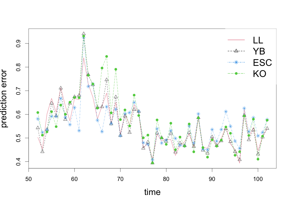
Refer to caption
Figure 6: Prediction errors at each time point for each method. LL, YB, ESC and KO represent the methods proposed in this paper, Yu and Bien 2017, Lee et al. 2019 and Khare et al. 2019, respectively.

We further illustrate the performance of LANCE prior in a classification problem. The GunPointAgeSpan data set, which is publicly available at http://timeseriesclassification.com, is used to conduct the quadratic discriminant analysis (QDA). This consists of the two GunPoint data sets released in 2003 and 2018, respectively, and each year, the same two actors (one male and one female) participated in the experiment. There are two classes in a data set: Gun and Point. For the Gun class, the actors hold a gun and point the gun toward a target, while they point with just their fingers (without a gun) in the Point class. The x-axis coordinates of centroid of the hand are recorded over five seconds of the movement based on 30 frames per second, which results in 150 frames (p=150)(p=150) per action.  Thus, this data set also has a time ordering between the variables. The GunPointAgeSpan has 135 training set (n=135)(n=135) and 316 test set, and the purpose of the analysis is to classify test observations into the two classes (Gun and Point). The numbers of observations corresponding to the Gun class are 68 and 160 in the training and test data, respectively. The training and test data sets are centered.

For each data xx in the test set, the quadratic discriminant score δk​(x)\delta_{k}(x) is calculated as follows:

δk​(x)\displaystyle\delta_{k}(x) =\displaystyle= 12​log​det(Ωk)−12​(x−μk)T​Ωk​(x−μk)+log⁡(nkn),k=1,2,\displaystyle\frac{1}{2}\log\det(\Omega_{k})-\frac{1}{2}(x-{\mu}_{k})^{T}\Omega_{k}(x-{\mu}_{k})+\log\Big(\frac{n_{k}}{n}\Big),\quad k=1,2,

where μk\mu_{k} and Ωk\Omega_{k} are the mean vector and precision matrix for the class k=1,2k=1,2, respectively. Here, nkn_{k} is the number of observations for the class kk, thus we have n1=68n_{1}=68 and n2=67n_{2}=67. To conduct the QDA, we estimate the unknown parameters μk\mu_{k} and Ωk\Omega_{k} using the training data set. They are plugged into δk​(x)\delta_{k}(x) similarly to the phone call center data example, and xx is then classified as the class k^=argmaxkδk​(x)\hat{k}=\argmax_{k}\delta_{k}(x). The performances of LANCE prior, YB method, ESC prior and CSCS method are compared, where cross-validation is used for each method except ESC prior.

Table 1: Classification errors for the test set in the GunPointAgeSpan data.
LL YB ESC KO
Error 0.2310 0.3956 0.2437 0.3704

Table 1 represents classification errors for the test set based the QDA using Ω^k\hat{\Omega}_{k} estimated by each method. For this data set, Bayesian methods seem to achieve lower classification errors than the penalized likelihood approaches, while LANCE prior achieves the lowest classification error. Despite similar performance, LANCE prior has a clear advantage over ESC prior by enabling a scalable cross-validation to select the hyperparameter. In practice, there is no guideline for choosing the hyperparameters in ESC prior, which can dramatically affect the performance.

5 Discussion

In this paper, we propose a Bayesian procedure for high-dimensional local dependence learning, where variables close to each other are more likely to be correlated. The proposed prior, LANCE prior, allows an exact computation of posteriors, which enables scalable inference even in high-dimensional settings. Furthermore, it provides a scalable Bayesian cross-validation to choose the hyperparameters. We establish selection consistency for the local dependence structure and posterior convergence rates for the Cholesky factor. The required conditions for these theoretical results are significantly weakened compared with the existing literature. Simulation studies in various settings show that LANCE prior outperforms other contenders in terms of the ROC curve, cross-validation-based analysis and computation time. Two real data analyses based on the phone call center and gun point data illustrate the satisfactory performance of the proposed method in linear prediction and classification problems, respectively.

It is worth mentioning that LANCE prior is only applicable when kjk_{j} is smaller than nn due to (𝐗j⁡(kj)T​𝐗j⁡(kj))−1({\bf X}_{j(k_{j})}^{T}{\bf X}_{j(k_{j})})^{-1} term in the conditional prior for aj(kj)a_{j}^{(k_{j})}. Although we rule out this situation by introducing condition (A3), in practice, we can modify LANCE prior to allow kj>nk_{j}>n when needed. Specifically, we can modify the conditional prior for aj(kj)a_{j}^{(k_{j})} to

aj(kj)|dj,kj\displaystyle a_{j}^{(k_{j})}\mid d_{j},k_{j} ∼i​n​d.\displaystyle\overset{ind.}{\sim} Nkj​(a~j(kj),djγ​(𝐗j⁡(kj)T​𝐗j⁡(kj)+c​Ikj)−1),j=2,…,p,\displaystyle N_{k_{j}}\Big(\tilde{a}_{j}^{(k_{j})},\frac{d_{j}}{\gamma}\big({\bf X}_{j(k_{j})}^{T}{\bf X}_{j(k_{j})}+cI_{k_{j}}\big)^{-1}\Big),\,\,j=2,\ldots,p, (6)

for some constant c>0c>0, where a~j(kj)=(𝐗j⁡(kj)T​𝐗j⁡(kj)+c​Ikj)−1​𝐗j⁡(kj)T​X~j\tilde{a}_{j}^{(k_{j})}=\big({\bf X}_{j(k_{j})}^{T}{\bf X}_{j(k_{j})}+cI_{k_{j}}\big)^{-1}{\bf X}_{j(k_{j})}^{T}\tilde{X}_{j}. Note that the above prior (6) has a variance stabilizing term c​IkjcI_{k_{j}}. Then, the resulting α\alpha-fractional posterior has the following closed form:

aj(kj)|dj,kj,𝐗n∼i​n​d.Nkj({𝐗j⁡(kj)T𝐗j⁡(kj)+c​γα+γIkj}−1𝐗j⁡(kj)TX~j,OPENdj​{(α+γ)​𝐗j⁡(kj)T​𝐗j⁡(kj)+c​γ​Ikj}−1),j=2,…,p,dj|kj,𝐗n∼i​n​d.​I​G​(α​n+ν02,α​n2​d~j(kj)),j=1,…,p,πα​(kj∣𝐗n)∝π⁡(kj)​{(𝐗j⁡(kj)T​𝐗j⁡(kj)+c​Ikj)−1​(𝐗j⁡(kj)T​𝐗j⁡(kj)+c​γα+γ​Ikj)}−kj2×(1+αγ)−kj2​(d~j(kj))−α​n+ν02,j=2,…,p,\displaystyle\begin{split}a_{j}^{(k_{j})}\mid d_{j},k_{j},{\bf X}_{n}\,\,&\overset{ind.}{\sim}\,\,N_{k_{j}}\Big(\big\{{\bf X}_{j(k_{j})}^{T}{\bf X}_{j(k_{j})}+\frac{c\gamma}{\alpha+\gamma}I_{k_{j}}\big\}^{-1}{\bf X}_{j(k_{j})}^{T}\tilde{X}_{j},\\ &\hskip 76.82234ptd_{j}\big\{(\alpha+\gamma){\bf X}_{j(k_{j})}^{T}{\bf X}_{j(k_{j})}+c\gamma I_{k_{j}}\big\}^{-1}\Big),\,\,j=2,\ldots,p,\\ d_{j}\mid k_{j},{\bf X}_{n}\,\,&\overset{ind.}{\sim}\,\,IG\Big(\frac{\alpha n+\nu_{0}}{2},\,\frac{\alpha n}{2}\tilde{d}_{j}^{(k_{j})}\Big),\,\,j=1,\ldots,p,\\ \pi_{\alpha}(k_{j}\mid{\bf X}_{n})\,\,&\propto\,\,\pi(k_{j})\Big\{\big({\bf X}_{j(k_{j})}^{T}{\bf X}_{j(k_{j})}+cI_{k_{j}}\big)^{-1}\big({\bf X}_{j(k_{j})}^{T}{\bf X}_{j(k_{j})}+\frac{c\gamma}{\alpha+\gamma}I_{k_{j}}\big)\Big\}^{-\frac{k_{j}}{2}}\\ &\hskip 28.45274pt\times\Big(1+\frac{\alpha}{\gamma}\Big)^{-\frac{k_{j}}{2}}\big(\tilde{d}_{j}^{(k_{j})}\big)^{-\frac{\alpha n+\nu_{0}}{2}},\,\,j=2,\ldots,p,\end{split}

where

d~j(kj)=n−1​X~jT​{In−𝐗j⁡(kj)​(𝐗j⁡(kj)T​𝐗j⁡(kj)+c​γα+γ​Ikj)−1​𝐗j⁡(kj)T}​X~j+\displaystyle\tilde{d}_{j}^{(k_{j})}=n^{-1}\tilde{X}_{j}^{T}\big\{I_{n}-{\bf X}_{j(k_{j})}\big({\bf X}_{j(k_{j})}^{T}{\bf X}_{j(k_{j})}+\frac{c\gamma}{\alpha+\gamma}I_{k_{j}}\big)^{-1}{\bf X}_{j(k_{j})}^{T}\big\}\tilde{X}_{j}+\hskip 56.9055pt
X~jT​𝐗j⁡(kj)​{(𝐗j⁡(kj)T​𝐗j⁡(kj)+c​γα+γ​Ikj)−1−(𝐗j⁡(kj)T​𝐗j⁡(kj)+c​Ikj)−1}​𝐗j⁡(kj)T​X~j​γ/(α​n).\displaystyle\tilde{X}_{j}^{T}{\bf X}_{j(k_{j})}\big\{\big({\bf X}_{j(k_{j})}^{T}{\bf X}_{j(k_{j})}+\frac{c\gamma}{\alpha+\gamma}I_{k_{j}}\big)^{-1}-({\bf X}_{j(k_{j})}^{T}{\bf X}_{j(k_{j})}+cI_{k_{j}})^{-1}\big\}{\bf X}_{j(k_{j})}^{T}\tilde{X}_{j}\,\gamma/(\alpha n).

Thus, the proposed LANCE prior can be modified to allow large bandwidths such that kj>nk_{j}>n. A sufficiently small c>0c>0 would give similar results with (5) in practice, although theoretical properties of the resulting α\alpha-fractional posterior should be further investigated.

An important and interesting future direction is to consider the estimation of covariance or precision structures with an unknown topological ordering on the variables of a DAG. Assume one specifies an arbitrary label of the variables as x1,…,xpx_{1},\ldots,x_{p} which does not necessarily correspond to the ordered variables. Let σ∈𝒮p\sigma\in\mathcal{S}_{p} be an element in the permutation group of pp variables and GσG_{\sigma} is the corresponding true DAG structure. If one is interested in learning both the DAG GσG_{\sigma} and the resulting covariance structure, a natural attempt is to impose a prior on the DAG GG along with a prior on the covariance structure given σ\sigma or the DAG, and then perform posterior inference. However, some identifiability conditions need to be imposed for the identifiability of the DAG structure. Please see Theorem 2.2 of Park and Kim 2020 for a state-of-the-art result on the identifiability of a Gaussian DAG, which essentially says that a Gaussian DAG is identifiable if the uncertainty level of a node jj is smaller than that of its descendants, given the non-descendants. One can potentially design a prior for the variances (djd_{j}s in our notation) that satisfies this ordered constraint. It would be interesting to study the posterior contraction and model selection properties of this model and design efficient MCMC algorithms.

If one does not impose any identifiability conditions (e.g., through the prior), another direction to deal with the unknown ordering case is to learn the equivalent class (or a representative of the class) of a DAG for all σ\sigmas, the so-called structure learning of DAGs which will learn the covariance structure of an equivalent class without learning the topological ordering of the variable or the underlying DAG structure. A recent work Zhou and Chang 2021 is one such example. The key ideas are the following: Let Np​(0,Σ∗)N_{p}(0,\Sigma^{*}) be the distribution of some true Gaussian DAG model G∗G^{*}. One can show that (see definition 7 in Zhou and Chang 2021 for example), for any σ∈𝒮p\sigma\in\mathcal{S}_{p}, one can have the Cholesky factor matrix Aσ∗A_{\sigma}^{*} and the positive diagonal matrix Dσ∗D_{\sigma}^{*} such that Σ∗=(Ip−Aσ∗)−1​Dσ∗​(Ip−(Aσ∗)T)−1\Sigma^{*}=(I_{p}-A_{\sigma}^{*})^{-1}D_{\sigma}^{*}(I_{p}-(A_{\sigma}^{*})^{T})^{-1}. That is, for any σ\sigma, one can find a unique pair (Aσ∗A_{\sigma}^{*}, OPENDσ∗)D_{\sigma}^{*}) which corresponds to some DAG Gσ∗G_{\sigma}^{*} called minimal I-map of the equivalent classes which has the same covariance structure as G∗G^{*}. This minimal I-map can be viewed as a representative point of the equivalent class which can be uniquely constructed. The structure learning problems boil down to the learnings of {Gσ∗,σ∈𝒮p}\{G_{\sigma}^{*},\sigma\in\mathcal{S}_{p}\} essentially. One can design appropriate priors that can obtain posterior consistency over {Gσ∗,σ∈𝒮p}\{G_{\sigma}^{*},\sigma\in\mathcal{S}_{p}\}.

Another work that deals with unknown ordering is Cao and Zhang 2020 which proposed to sample KK permutation matrices or σ\sigmas under the MCD model. They obtained the posterior estimates of the Cholesky factors and diagonal matrices for each permutation which are then averaged to obtain a final estimate of the precision matrix.

Acknowledgement

We are very grateful to the Associate Editor and the two reviewers for their valuable comments which have led to great improvement in our paper. We would also like to thank Guo (Hugo) Yu for very helpful discussions.

Appendix

Appendix A Proofs

Note that

πα​(kj≠k0​j​ for at least one ​2≤j≤p∣𝐗n)\displaystyle\pi_{\alpha}\big(k_{j}\neq k_{0j}\text{ for at least one }2\leq j\leq p\mid{\bf X}_{n}\big)
≤\displaystyle\leq ∑j=2pπα​(kj≠k0​j∣𝐗n)\displaystyle\sum_{j=2}^{p}\pi_{\alpha}(k_{j}\neq k_{0j}\mid{\bf X}_{n})
=\displaystyle= ∑j=2p{πα​(kj>k0​j∣𝐗n)+πα​(kj<k0​j∣𝐗n)}.\displaystyle\sum_{j=2}^{p}\Big\{\pi_{\alpha}(k_{j}>k_{0j}\mid{\bf X}_{n})+\pi_{\alpha}(k_{j}<k_{0j}\mid{\bf X}_{n})\Big\}.

We first show that

∑j=2p𝔼0​{πα​(kj>k0​j∣𝐗n)}\displaystyle\sum_{j=2}^{p}\mathbb{E}_{0}\big\{\pi_{\alpha}(k_{j}>k_{0j}\mid{\bf X}_{n})\big\} ⟶\displaystyle\longrightarrow 0\displaystyle 0

as n→∞n\to\infty. For any kj>k0​jk_{j}>k_{0j}, we have

πα​(kj∣𝐗n)\displaystyle\pi_{\alpha}(k_{j}\mid{\bf X}_{n}) ≤\displaystyle\leq πα​(kj∣𝐗n)πα​(k0​j∣𝐗n)\displaystyle\frac{\pi_{\alpha}(k_{j}\mid{\bf X}_{n})}{\pi_{\alpha}(k_{0j}\mid{\bf X}_{n})}
≤\displaystyle\leq π⁡(kj)π⁡(k0​j)​(1+αγ)−kj−k0​j2​(d^j(kj)d^j(k0​j))−α​n+ν02.\displaystyle\frac{\pi(k_{j})}{\pi(k_{0j})}\Big(1+\frac{\alpha}{\gamma}\Big)^{-\frac{k_{j}-k_{0j}}{2}}\Bigg(\frac{\widehat{d}_{j}^{(k_{j})}}{\widehat{d}_{j}^{(k_{0j})}}\Bigg)^{-\frac{\alpha n+\nu_{0}}{2}}.

Furthermore, it is easy to see that d^j(kj)/d^j(k0​j)∼B​e​t​a​((n−kj)/2,(kj−k0​j)/2)\widehat{d}_{j}^{(k_{j})}/\widehat{d}_{j}^{(k_{0j})}\sim Beta((n-k_{j})/2,(k_{j}-k_{0j})/2) for any 1≤j≤p1\leq j\leq p because

n​d0​j−1​d^j(kj)\displaystyle nd_{0j}^{-1}\widehat{d}_{j}^{(k_{j})} =\displaystyle= d0​j−1​X~jT​(In−P~j​kj)​X~j∼χn−kj2,\displaystyle d_{0j}^{-1}\tilde{X}_{j}^{T}(I_{n}-\tilde{P}_{jk_{j}})\tilde{X}_{j}\sim\chi_{n-k_{j}}^{2},
n​d0​j−1​d^j(k0​j)\displaystyle nd_{0j}^{-1}\widehat{d}_{j}^{(k_{0j})} ≡𝑑\displaystyle\overset{d}{\equiv} n​d0​j−1​d^j(kj)⊕χkj−k0​j2.\displaystyle nd_{0j}^{-1}\widehat{d}_{j}^{(k_{j})}\oplus\chi_{k_{j}-k_{0j}}^{2}.

Thus,

𝔼0​(d^j(kj)d^j(k0​j))−α​n+ν02\displaystyle\mathbb{E}_{0}\Bigg(\frac{\widehat{d}_{j}^{(k_{j})}}{\widehat{d}_{j}^{(k_{0j})}}\Bigg)^{-\frac{\alpha n+\nu_{0}}{2}} =\displaystyle= Γ⁡(n−k0​j2)​Γ​(n⁡(1−α)−ν0−kj2)Γ⁡(n−kj2)​Γ​(n⁡(1−α)−ν0−k0​j2)\displaystyle\frac{\Gamma\Big(\frac{n-k_{0j}}{2}\Big)\Gamma\Big(\frac{n(1-\alpha)-\nu_{0}-k_{j}}{2}\Big)}{\Gamma\Big(\frac{n-k_{j}}{2}\Big)\Gamma\Big(\frac{n(1-\alpha)-\nu_{0}-k_{0j}}{2}\Big)}
≤\displaystyle\leq (21−α)kj−k0​j2,\displaystyle\Big(\frac{2}{1-\alpha}\Big)^{\frac{k_{j}-k_{0j}}{2}},

because we assume that ν0=O⁡(1)\nu_{0}=O(1) and Rj≤n⁡(1−α)/2R_{j}\leq n(1-\alpha)/2. This implies that

∑j=2p𝔼0​{πα​(kj>k0​j∣𝐗n)}\displaystyle\sum_{j=2}^{p}\mathbb{E}_{0}\big\{\pi_{\alpha}(k_{j}>k_{0j}\mid{\bf X}_{n})\big\} =\displaystyle= ∑j=2p∑kj=k0​j+1Rj𝔼0​{πα​(kj∣𝐗n)}\displaystyle\sum_{j=2}^{p}\sum_{k_{j}=k_{0j}+1}^{R_{j}}\mathbb{E}_{0}\big\{\pi_{\alpha}(k_{j}\mid{\bf X}_{n})\big\}
≤\displaystyle\leq ∑j=2p∑kj=k0​j+1Rj(cα,γc1​pc2)kj−k0​j\displaystyle\sum_{j=2}^{p}\sum_{k_{j}=k_{0j}+1}^{R_{j}}\Big(\frac{c_{\alpha,\gamma}}{c_{1}p^{c_{2}}}\Big)^{k_{j}-k_{0j}}
≲\displaystyle\lesssim ∑j=2pcα,γc1​pc2,\displaystyle\sum_{j=2}^{p}\frac{c_{\alpha,\gamma}}{c_{1}p^{c_{2}}},

where cα,γ=(1+α/γ)−1/2{2/(1−α)}1/2c_{\alpha,\gamma}=(1+\alpha/\gamma)^{-1/2}\{2/(1-\alpha)\}^{1/2}. The last term is of order o⁡(1)o(1) because we assume that c2>1c_{2}>1.

Now we show that

∑j=2p𝔼0​{πα​(kj<k0​j∣𝐗n)}\displaystyle\sum_{j=2}^{p}\mathbb{E}_{0}\big\{\pi_{\alpha}(k_{j}<k_{0j}\mid{\bf X}_{n})\big\} ⟶\displaystyle\longrightarrow 0\displaystyle 0

as n→∞n\to\infty. For given integer 2≤j≤p2\leq j\leq p and constant ϵ={(1−α)/10}2\epsilon=\{(1-\alpha)/10\}^{2}, define the sets

Njc\displaystyle N_{j}^{c} =\displaystyle= {𝐗n:λmax(Ω0​n)−1(1−2ϵ)2≤n−1λmin(𝐗j⁡(k0​j)T𝐗j⁡(k0​j))\displaystyle\Big\{{\bf X}_{n}:\lambda_{\max}(\Omega_{0n})^{-1}(1-2\epsilon)^{2}\leq n^{-1}\lambda_{\min}({\bf X}_{j(k_{0j})}^{T}{\bf X}_{j(k_{0j})})
≤n−1λmax(𝐗j⁡(k0​j)T𝐗j⁡(k0​j))≤λmin(Ω0​n)−1(1+2ϵ)2},\displaystyle\quad\quad\quad\quad\quad\leq n^{-1}\lambda_{\max}({\bf X}_{j(k_{0j})}^{T}{\bf X}_{j(k_{0j})})\leq\lambda_{\min}(\Omega_{0n})^{-1}(1+2\epsilon)^{2}\Big\},
N1​jc\displaystyle N_{1j}^{c} =\displaystyle= {𝐗n:|d^j(k0​j)d0​j−1|∈(−4​ϵ​n−k0​jn−k0​jn, 4​ϵ​n−k0​jn−k0​jn)},\displaystyle\Big\{{\bf X}_{n}:\Big|\frac{\widehat{d}_{j}^{(k_{0j})}}{d_{0j}}-1\Big|\in\Big(-4\sqrt{\epsilon}\frac{n-k_{0j}}{n}-\frac{k_{0j}}{n},\,4\sqrt{\epsilon}\frac{n-k_{0j}}{n}-\frac{k_{0j}}{n}\Big)\Big\},
N2​j​kjc\displaystyle N_{2jk_{j}}^{c} =\displaystyle= {𝐗n:0<d^j(kj)−d^j(k0​j)d0​j<ϵ+λ^j​kjn},\displaystyle\Big\{{\bf X}_{n}:0<\frac{\widehat{d}_{j}^{(k_{j})}-\widehat{d}_{j}^{(k_{0j})}}{d_{0j}}<\epsilon+\frac{\widehat{\lambda}_{jk_{j}}}{n}\Big\},

where

λ^j​kj\displaystyle\widehat{\lambda}_{jk_{j}} =\displaystyle= 1d0​j​‖(In−P~j​kj)​𝐗j⁡(k0​j)​a0​j(k0​j)‖22.\displaystyle\frac{1}{d_{0j}}\|(I_{n}-\tilde{P}_{jk_{j}}){\bf X}_{j(k_{0j})}a_{0j}^{(k_{0j})}\|_{2}^{2}.

Let Nj​kjc=Njc∩N1​jc∩N2​j​kjcN_{jk_{j}}^{c}=N_{j}^{c}\cap N_{1j}^{c}\cap N_{2jk_{j}}^{c} for all 2≤j≤p2\leq j\leq p. Since

∑j=2p𝔼0​{πα​(kj<k0​j∣𝐗n)}\displaystyle\sum_{j=2}^{p}\mathbb{E}_{0}\big\{\pi_{\alpha}(k_{j}<k_{0j}\mid{\bf X}_{n})\big\}
≤\displaystyle\leq ∑j=2p∑kj<k0​jℙ0​(Nj​kj)+∑j=2p∑kj<k0​j𝔼0​{πα​(kj∣𝐗n)πα​(k0​j∣𝐗n)​I​(Nj​kjc)}\displaystyle\sum_{j=2}^{p}\sum_{k_{j}<k_{0j}}\mathbb{P}_{0}(N_{jk_{j}})+\sum_{j=2}^{p}\sum_{k_{j}<k_{0j}}\mathbb{E}_{0}\Big\{\frac{\pi_{\alpha}(k_{j}\mid{\bf X}_{n})}{\pi_{\alpha}(k_{0j}\mid{\bf X}_{n})}I(N_{jk_{j}}^{c})\Big\}
≤\displaystyle\hskip-8.5359pt\leq ∑j=2p∑kj<k0​jℙ0​(Nj​kj)+∑j=2p∑kj<k0​j𝔼0​{π⁡(kj)π⁡(k0​j)​(1+αγ)k0​j−kj​(d^j(kj)d^j(k0​j))−α​n+ν02​I​(Nj​kjc)},\displaystyle\hskip-8.5359pt\sum_{j=2}^{p}\sum_{k_{j}<k_{0j}}\mathbb{P}_{0}(N_{jk_{j}})+\sum_{j=2}^{p}\sum_{k_{j}<k_{0j}}\mathbb{E}_{0}\Bigg\{\frac{\pi(k_{j})}{\pi(k_{0j})}\Big(1+\frac{\alpha}{\gamma}\Big)^{k_{0j}-k_{j}}\Bigg(\frac{\widehat{d}_{j}^{(k_{j})}}{\widehat{d}_{j}^{(k_{0j})}}\Bigg)^{-\frac{\alpha n+\nu_{0}}{2}}I(N_{jk_{j}}^{c})\Bigg\},

we will complete the proof by showing that

∑j=2p∑kj<k0​jℙ0​(Nj​kj)\displaystyle\sum_{j=2}^{p}\sum_{k_{j}<k_{0j}}\mathbb{P}_{0}(N_{jk_{j}}) ⟶\displaystyle\longrightarrow 0\displaystyle 0 (7)

and

∑j=2p∑kj<k0​j𝔼0​{π⁡(kj)π⁡(k0​j)​(1+αγ)k0​j−kj​(d^j(kj)d^j(k0​j))−α​n+ν02​I​(Nj​kjc)}\displaystyle\sum_{j=2}^{p}\sum_{k_{j}<k_{0j}}\mathbb{E}_{0}\Bigg\{\frac{\pi(k_{j})}{\pi(k_{0j})}\Big(1+\frac{\alpha}{\gamma}\Big)^{k_{0j}-k_{j}}\Bigg(\frac{\widehat{d}_{j}^{(k_{j})}}{\widehat{d}_{j}^{(k_{0j})}}\Bigg)^{-\frac{\alpha n+\nu_{0}}{2}}I(N_{jk_{j}}^{c})\Bigg\} ⟶\displaystyle\longrightarrow 0\displaystyle 0 (8)

as n→∞n\to\infty.

To show (7), it suffices to show that

∑j=2p∑kj<k0​j{ℙ0​(Nj)+ℙ0​(N1​j)+ℙ0​(N2​j​kj)}\displaystyle\sum_{j=2}^{p}\sum_{k_{j}<k_{0j}}\Big\{\mathbb{P}_{0}(N_{j})+\mathbb{P}_{0}(N_{1j})+\mathbb{P}_{0}(N_{2jk_{j}})\Big\} ⟶\displaystyle\longrightarrow 0\displaystyle 0

as n→∞n\to\infty. Note that

∑j=2p∑kj<k0​jℙ0​(Nj)\displaystyle\sum_{j=2}^{p}\sum_{k_{j}<k_{0j}}\mathbb{P}_{0}(N_{j}) ≤\displaystyle\leq ∑j=2p∑kj<k0​j4​exp⁡(−n​ϵ22)\displaystyle\sum_{j=2}^{p}\sum_{k_{j}<k_{0j}}4\exp\Big(-\frac{n\epsilon^{2}}{2}\Big)
≤\displaystyle\leq ∑j=2p4​exp⁡(−n​ϵ22+log⁡k0​j)\displaystyle\sum_{j=2}^{p}4\exp\Big(-\frac{n\epsilon^{2}}{2}+\log k_{0j}\Big)
≤\displaystyle\leq 4​exp⁡(−n​ϵ22+2​log⁡p)=o⁡(1)\displaystyle 4\exp\Big(-\frac{n\epsilon^{2}}{2}+2\log p\Big)\,\,=\,\,o(1)

for all sufficiently large nn, where the first inequality follows from Corollary 5.35 in Eldar and Kutyniok 2012. Since n​d^j(k0​j)/d0​j∼χn−k0​j2n\widehat{d}_{j}^{(k_{0j})}/d_{0j}\sim\chi^{2}_{n-k_{0j}}, we have

∑j=2p∑kj<k0​jℙ0​(N1​j)\displaystyle\sum_{j=2}^{p}\sum_{k_{j}<k_{0j}}\mathbb{P}_{0}(N_{1j}) ≤\displaystyle\leq ∑j=2p∑kj<k0​j2​exp⁡{−ϵ⁡(n−k0​j)}\displaystyle\sum_{j=2}^{p}\sum_{k_{j}<k_{0j}}2\exp\{-\epsilon(n-k_{0j})\}
≤\displaystyle\leq ∑j=2p2​exp⁡{−ϵ⁡(n−k0​j)+log⁡k0​j}\displaystyle\sum_{j=2}^{p}2\exp\{-\epsilon(n-k_{0j})+\log k_{0j}\}
≤\displaystyle\leq 2​exp⁡(−ϵ​n2+2​log⁡p)=o⁡(1)\displaystyle 2\exp\Big(-\frac{\epsilon n}{2}+2\log p\Big)\,\,=\,\,o(1)

for all sufficiently large nn, by the concentration inequality for chi-square random variables in Lemma 1 of Laurent and Massart 2000. Furthermore, because n⁡(d^j(kj)−d^j(k0​j))/d0​j∼χk0​j−kj2​(λ^j​kj)n(\widehat{d}_{j}^{(k_{j})}-\widehat{d}_{j}^{(k_{0j})})/d_{0j}\sim\chi^{2}_{k_{0j}-k_{j}}(\widehat{\lambda}_{jk_{j}}), where χm2​(λ)\chi_{m}^{2}(\lambda) denotes the noncentral chi-square distribution with the degrees of freedom mm and the noncentrality parameter λ\lambda, we have

∑j=2p∑kj<k0​jℙ0​(N2​kj)\displaystyle\sum_{j=2}^{p}\sum_{k_{j}<k_{0j}}\mathbb{P}_{0}(N_{2k_{j}})
≲\displaystyle\lesssim ∑j=2p∑kj<k0​j[{ϵ​n2​(k0​j−kj)}k0​j−kj2​exp⁡(k0​j−kj2−ϵ​n2)+𝔼0​(λ^j​kjϵ​n​e−ϵ2​n232​λ^j​kj∧1)]\displaystyle\sum_{j=2}^{p}\sum_{k_{j}<k_{0j}}\left[\Big\{\frac{\epsilon n}{2(k_{0j}-k_{j})}\Big\}^{\frac{k_{0j}-k_{j}}{2}}\exp\Big(\frac{k_{0j}-k_{j}}{2}-\frac{\epsilon n}{2}\Big)+\mathbb{E}_{0}\Big(\frac{\widehat{\lambda}_{jk_{j}}}{\epsilon n}e^{-\frac{\epsilon^{2}n^{2}}{32\widehat{\lambda}_{jk_{j}}}}\wedge 1\Big)\right]
≤\displaystyle\leq ∑j=2p∑kj<k0​j[exp⁡(−ϵ​n4)+𝔼0​{λ^j​kjϵ​n​e−ϵ2​n232​λ^j​kj​I​(Njc)}+ℙ0​(Nj)]\displaystyle\sum_{j=2}^{p}\sum_{k_{j}<k_{0j}}\left[\exp\Big(-\frac{\epsilon n}{4}\Big)+\mathbb{E}_{0}\Big\{\frac{\widehat{\lambda}_{jk_{j}}}{\epsilon n}e^{-\frac{\epsilon^{2}n^{2}}{32\widehat{\lambda}_{jk_{j}}}}I(N_{j}^{c})\Big\}+\mathbb{P}_{0}(N_{j})\right]
≤\displaystyle\leq ∑j=2p∑kj<k0​j[exp⁡(−ϵ​n4)+exp⁡{−ϵ2​n​λmax​(Ω0​n)−1​λmin​(Ω0​n)128​(1+2​ϵ)2}+4​exp⁡(−n​ϵ22)]\displaystyle\sum_{j=2}^{p}\sum_{k_{j}<k_{0j}}\left[\exp\Big(-\frac{\epsilon n}{4}\Big)+\exp\Big\{-\frac{\epsilon^{2}n\lambda_{\max}(\Omega_{0n})^{-1}\lambda_{\min}(\Omega_{0n})}{128(1+2\epsilon)^{2}}\Big\}+4\exp\Big(-\frac{n\epsilon^{2}}{2}\Big)\right]
=\displaystyle= o⁡(1)\displaystyle o(1)

by Lemma 4 of Shin et al. 2018 and conditions (A1), (A3) and (A4). The last inequality holds because

λ^j​kj\displaystyle\widehat{\lambda}_{jk_{j}} ≤\displaystyle\leq λmax​(𝐗j⁡(k0​j)T​𝐗j⁡(k0​j))​d0​j−1​‖a0​j(k0​j)‖22\displaystyle\lambda_{\max}({\bf X}_{j(k_{0j})}^{T}{\bf X}_{j(k_{0j})})d_{0j}^{-1}\|a_{0j}^{(k_{0j})}\|_{2}^{2}
≤\displaystyle\leq nλmin(Ω0​n)−1(1+2ϵ)2{d0​j−1+∥d0​j−1/2(ej−a0​j)∥22}\displaystyle n\lambda_{\min}(\Omega_{0n})^{-1}(1+2\epsilon)^{2}\big\{d_{0j}^{-1}+\|d_{0j}^{-1/2}(e_{j}-a_{0j})\|_{2}^{2}\big\}
≤\displaystyle\leq 2​n​λmin​(Ω0​n)−1​(1+2​ϵ)2​λmax​(Ω0​n),\displaystyle 2n\lambda_{\min}(\Omega_{0n})^{-1}(1+2\epsilon)^{2}\lambda_{\max}(\Omega_{0n}),

where eje_{j} is the unit vector whose the jjth element is 1 and the others are zero. Thus, we have proved (7).

Now, we complete the proof by showing (8). For a given kj<k0​jk_{j}<k_{0j}, because −log⁡(1−x)≤x/(1−x)-\log(1-x)\leq x/(1-x) for any x<1x<1, it can be shown that

(d^j(kj)d^j(k0​j))−α​n+ν02\displaystyle\Bigg(\frac{\widehat{d}_{j}^{(k_{j})}}{\widehat{d}_{j}^{(k_{0j})}}\Bigg)^{-\frac{\alpha n+\nu_{0}}{2}} =\displaystyle= (1−d^j(k0​j)−d^j(kj)d^j(k0​j))−α​n+ν02\displaystyle\Bigg(1-\frac{\widehat{d}_{j}^{(k_{0j})}-\widehat{d}_{j}^{(k_{j})}}{\widehat{d}_{j}^{(k_{0j})}}\Bigg)^{-\frac{\alpha n+\nu_{0}}{2}}
≤\displaystyle\leq exp⁡{α+ν0n2​d0​j​(1+Q^j​kj)​n​(d^j(k0​j)−d^j(kj))},\displaystyle\exp\Bigg\{\frac{\alpha+\frac{\nu_{0}}{n}}{2d_{0j}(1+\widehat{Q}_{jk_{j}})}n\Big(\widehat{d}_{j}^{(k_{0j})}-\widehat{d}_{j}^{(k_{j})}\Big)\Bigg\},

where

Q^j​kj\displaystyle\widehat{Q}_{jk_{j}} =\displaystyle= d^j(k0​j)d0​j−1+d^j(kj)−d^j(k0​j)d0​j.\displaystyle\frac{\widehat{d}_{j}^{(k_{0j})}}{d_{0j}}-1+\frac{\widehat{d}_{j}^{(k_{j})}-\widehat{d}_{j}^{(k_{0j})}}{d_{0j}}.

Then, we have

Q^j​kj\displaystyle\widehat{Q}_{jk_{j}} ≤\displaystyle\leq 4​ϵ​n−k0​jn−k0​jn+ϵ+λ^j​kjn≤  5​ϵ+λ^j​kjn=:Q^1​j,\displaystyle 4\sqrt{\epsilon}\frac{n-k_{0j}}{n}-\frac{k_{0j}}{n}+\epsilon+\frac{\widehat{\lambda}_{jk_{j}}}{n}\,\,\leq\,\,5\sqrt{\epsilon}+\frac{\widehat{\lambda}_{jk_{j}}}{n}\,\,=:\,\,\widehat{Q}_{1j},
Q^j​kj\displaystyle\widehat{Q}_{jk_{j}} ≥\displaystyle\geq −4​ϵ​n−k0​jn−k0​jn≥−5​ϵ=:Q^2​j\displaystyle-4\sqrt{\epsilon}\frac{n-k_{0j}}{n}-\frac{k_{0j}}{n}\,\,\geq\,\,-5\sqrt{\epsilon}\,\,=:\,\,\widehat{Q}_{2j}

on the event Nj​kjcN_{jk_{j}}^{c}. Further note that

n⁡(d^j(k0​j)−d^j(kj))\displaystyle n\big(\widehat{d}_{j}^{(k_{0j})}-\widehat{d}_{j}^{(k_{j})}\big)
=\displaystyle= X~jT​(P~j​kj−P~j​k0​j)​X~j\displaystyle\tilde{X}_{j}^{T}(\tilde{P}_{jk_{j}}-\tilde{P}_{jk_{0j}})\tilde{X}_{j}
≡𝑑\displaystyle\overset{d}{\equiv} −‖(In−P~j​kj)​𝐗j⁡(k0​j)​a0​j(k0​j)‖22−2​ϵ~jT​(In−P~j​kj)​𝐗j⁡(k0​j)​a0​j(k0​j)+ϵ~jT​(P~j​kj−P~j​k0​j)​ϵ~j\displaystyle-\|(I_{n}-\tilde{P}_{jk_{j}}){\bf X}_{j(k_{0j})}a_{0j}^{(k_{0j})}\|_{2}^{2}-2\tilde{\epsilon}_{j}^{T}(I_{n}-\tilde{P}_{jk_{j}}){\bf X}_{j(k_{0j})}a_{0j}^{(k_{0j})}+\tilde{\epsilon}_{j}^{T}(\tilde{P}_{jk_{j}}-\tilde{P}_{jk_{0j}})\tilde{\epsilon}_{j}
≤\displaystyle\leq −d0​j​λ^j​kj−2​ϵ~jT​(In−P~j​kj)​𝐗j⁡(k0​j)​a0​j(k0​j)\displaystyle-d_{0j}\widehat{\lambda}_{jk_{j}}-2\tilde{\epsilon}_{j}^{T}(I_{n}-\tilde{P}_{jk_{j}}){\bf X}_{j(k_{0j})}a_{0j}^{(k_{0j})}
=:\displaystyle=: −d0​j​λ^j​kj−2​Vj​kj,\displaystyle-d_{0j}\widehat{\lambda}_{jk_{j}}-2V_{jk_{j}},

where ϵ~j∼Nn​(0,d0​j​In)\tilde{\epsilon}_{j}\sim N_{n}(0,d_{0j}I_{n}) and Vj​kj/d0​j∼N⁡(0,d0​j​λ^j​kj)V_{jk_{j}}/\sqrt{d_{0j}}\sim N(0,d_{0j}\widehat{\lambda}_{jk_{j}}) under ℙ0\mathbb{P}_{0} given 𝐗j⁡(k0​j){\bf X}_{j(k_{0j})}. Then,

𝔼0​{(d^j(kj)d^j(k0​j))−α​n+ν02​I​(Nj​kjc)|𝐗j⁡(k0​j)}\displaystyle\mathbb{E}_{0}\left\{\Bigg(\frac{\widehat{d}_{j}^{(k_{j})}}{\widehat{d}_{j}^{(k_{0j})}}\Bigg)^{-\frac{\alpha n+\nu_{0}}{2}}I(N_{jk_{j}}^{c})\,\,\Big|\,\,{\bf X}_{j(k_{0j})}\right\}
≤\displaystyle\leq 𝔼0​[exp⁡{α+ν0n2​d0​j​(1+Q^j​kj)​n​(d^j(k0​j)−d^j(kj))}​I​(Nj​kjc)|𝐗j⁡(k0​j)]\displaystyle\mathbb{E}_{0}\left[\exp\Bigg\{\frac{\alpha+\frac{\nu_{0}}{n}}{2d_{0j}(1+\widehat{Q}_{jk_{j}})}n\Big(\widehat{d}_{j}^{(k_{0j})}-\widehat{d}_{j}^{(k_{j})}\Big)\Bigg\}I(N_{jk_{j}}^{c})\,\,\Big|\,\,{\bf X}_{j(k_{0j})}\right]
≤\displaystyle\leq 𝔼0​[∑Q^j​kj∈{Q^1​j,Q^2​j}exp⁡{−α+ν0n2​d0​j​(1+Q^j​kj)​(d0​j​λ^j​kj+2​Vj​kj)}​I​(Nj​kjc)|𝐗j⁡(k0​j)]\displaystyle\mathbb{E}_{0}\left[\sum_{\widehat{Q}_{jk_{j}}\in\{\widehat{Q}_{1j},\widehat{Q}_{2j}\}}\exp\Bigg\{-\frac{\alpha+\frac{\nu_{0}}{n}}{2d_{0j}(1+\widehat{Q}_{jk_{j}})}\Big(d_{0j}\widehat{\lambda}_{jk_{j}}+2V_{jk_{j}}\Big)\Bigg\}I(N_{jk_{j}}^{c})\,\,\Big|\,\,{\bf X}_{j(k_{0j})}\right]
≤\displaystyle\leq 2​exp⁡{−α+ν0n2​(1+5​ϵ+λ^j​kj/n)​(1−α+ν0n1−5​ϵ)​λ^j​kj}\displaystyle 2\exp\Big\{-\frac{\alpha+\frac{\nu_{0}}{n}}{2(1+5\sqrt{\epsilon}+\widehat{\lambda}_{jk_{j}}/n)}\Big(1-\frac{\alpha+\frac{\nu_{0}}{n}}{1-5\sqrt{\epsilon}}\Big)\widehat{\lambda}_{jk_{j}}\Big\}
≤\displaystyle\leq 2​exp⁡{−α+ν0n2​(1+5​ϵ+λ^j​kj/n)​(1−α+ν0n1−5​ϵ)​λ^j​kj}≡  2​Λ^j​kj,\displaystyle 2\exp\Big\{-\frac{\alpha+\frac{\nu_{0}}{n}}{2(1+5\sqrt{\epsilon}+\widehat{\lambda}_{jk_{j}}/n)}\Big(1-\frac{\alpha+\frac{\nu_{0}}{n}}{1-5\sqrt{\epsilon}}\Big)\widehat{\lambda}_{jk_{j}}\Big\}\,\,\equiv\,\,2\widehat{\Lambda}_{jk_{j}},

where the third inequality follows from the moment generating function of normal distribution. Note that

1−α+ν0n1−5​ϵ\displaystyle 1-\frac{\alpha+\frac{\nu_{0}}{n}}{1-5\sqrt{\epsilon}} >\displaystyle> 1−α−ν0n2,\displaystyle\frac{1-\alpha-\frac{\nu_{0}}{n}}{2},

and by Lemma 5 of Arias-Castro and Lounici 2014,

λ^j​kj\displaystyle\widehat{\lambda}_{jk_{j}} =\displaystyle= d0​j−1​‖(In−P~j​kj)​𝐗j⁡(k0​j)​a0​j(k0​j)‖22\displaystyle d_{0j}^{-1}\|(I_{n}-\tilde{P}_{jk_{j}}){\bf X}_{j(k_{0j})}a_{0j}^{(k_{0j})}\|_{2}^{2}
≥\displaystyle\geq λmin(𝐗j⁡(k0​j)T𝐗j⁡(k0​j))(k0​j−kj)min(j,l):a0,j​l≠0(a0,j​l2/d0​j)\displaystyle\lambda_{\min}({\bf X}_{j(k_{0j})}^{T}{\bf X}_{j(k_{0j})})(k_{0j}-k_{j})\min_{(j,l):a_{0,jl}\neq 0}(a_{0,jl}^{2}/d_{0j})
≥\displaystyle\geq nλmax(Ω0​n)−1(1−2ϵ)2(k0​j−kj)min(j,l):a0,j​l≠0(a0,j​l2/d0​j)\displaystyle n\lambda_{\max}(\Omega_{0n})^{-1}(1-2\epsilon)^{2}(k_{0j}-k_{j})\min_{(j,l):a_{0,jl}\neq 0}(a_{0,jl}^{2}/d_{0j})

on the event Nj​kjcN_{jk_{j}}^{c}. Therefore, on the event Nj​kjcN_{jk_{j}}^{c},

α+ν0n2​(1+5​ϵ+λ^j​kj/n)​(1−α+ν0n1−5​ϵ)​λ^j​kj\displaystyle\frac{\alpha+\frac{\nu_{0}}{n}}{2(1+5\sqrt{\epsilon}+\widehat{\lambda}_{jk_{j}}/n)}\Big(1-\frac{\alpha+\frac{\nu_{0}}{n}}{1-5\sqrt{\epsilon}}\Big)\widehat{\lambda}_{jk_{j}}
≥\displaystyle\geq 14​(α+ν0n)​(1−α−ν0n)​λ^j​kj1+5​ϵ+λ^j​kj/n\displaystyle\frac{1}{4}\Big(\alpha+\frac{\nu_{0}}{n}\Big)\Big(1-\alpha-\frac{\nu_{0}}{n}\Big)\frac{\widehat{\lambda}_{jk_{j}}}{1+5\sqrt{\epsilon}+\widehat{\lambda}_{jk_{j}}/n}
=\displaystyle= 14​(α+ν0n)​(1−α−ν0n)​(1+5​ϵλ^j​kj+1n)−1\displaystyle\frac{1}{4}\Big(\alpha+\frac{\nu_{0}}{n}\Big)\Big(1-\alpha-\frac{\nu_{0}}{n}\Big)\Big(\frac{1+5\sqrt{\epsilon}}{\widehat{\lambda}_{jk_{j}}}+\frac{1}{n}\Big)^{-1}
≥\displaystyle\geq 14(α+ν0n)(1−α−ν0n){(1+5​ϵ)​λmax​(Ω0​n)(1−2ϵ)2(k0​j−kj)min(j,l):a0,j​l≠0(a0,j​l2/d0​j)+1n}−1\displaystyle\frac{1}{4}\Big(\alpha+\frac{\nu_{0}}{n}\Big)\Big(1-\alpha-\frac{\nu_{0}}{n}\Big)\Big\{\frac{(1+5\sqrt{\epsilon})\lambda_{\max}(\Omega_{0n})}{(1-2\epsilon)^{2}(k_{0j}-k_{j})\min_{(j,l):a_{0,jl}\neq 0}(a_{0,jl}^{2}/d_{0j})}+\frac{1}{n}\Big\}^{-1}
≥\displaystyle\geq 14​(α+ν0n)​(1−α−ν0n)​{(1+5​ϵ)(1−2​ϵ)2​(k0​j−kj)​Cbm​log⁡p+1n}−1\displaystyle\frac{1}{4}\Big(\alpha+\frac{\nu_{0}}{n}\Big)\Big(1-\alpha-\frac{\nu_{0}}{n}\Big)\Big\{\frac{(1+5\sqrt{\epsilon})}{(1-2\epsilon)^{2}(k_{0j}-k_{j})C_{\rm bm}\log p}+\frac{1}{n}\Big\}^{-1}
≥\displaystyle\geq 18​(α+ν0n)​(1−α−ν0n)​(1−2​ϵ)2​(k0​j−kj)​Cbm​log⁡p1+5​ϵ\displaystyle\frac{1}{8}\Big(\alpha+\frac{\nu_{0}}{n}\Big)\Big(1-\alpha-\frac{\nu_{0}}{n}\Big)\frac{(1-2\epsilon)^{2}(k_{0j}-k_{j})C_{\rm bm}\log p}{1+5\sqrt{\epsilon}}
≥\displaystyle\geq (k0​j−kj)​Mbm​log⁡p\displaystyle(k_{0j}-k_{j})M_{\rm bm}\log p

for all sufficiently large nn and any 0.6≤α<10.6\leq\alpha<1, by conditions (A2) and (A4), where Cbm=10​Mbm/{(α+ν0/n)​(1−α−ν0/n)}C_{\rm bm}=10M_{\rm bm}/\{(\alpha+\nu_{0}/n)(1-\alpha-\nu_{0}/n)\}. It implies that

∑j=2p∑kj<k0​j𝔼0​{πα​(kj∣𝐗n)πα​(k0​j∣𝐗n)​I​(Nj​kjc)}\displaystyle\sum_{j=2}^{p}\sum_{k_{j}<k_{0j}}\mathbb{E}_{0}\Big\{\frac{\pi_{\alpha}(k_{j}\mid{\bf X}_{n})}{\pi_{\alpha}(k_{0j}\mid{\bf X}_{n})}I(N_{jk_{j}}^{c})\Big\}
≤\displaystyle\leq ∑j=2p∑kj<k0​j(c1​pc2)k0​j−kj​(1+αγ)k0​j−kj2​𝔼0​[Λ^j​kj​{I⁡(Nj​kjc)+I⁡(Nj​kj)}]\displaystyle\sum_{j=2}^{p}\sum_{k_{j}<k_{0j}}(c_{1}p^{c_{2}})^{k_{0j}-k_{j}}\Big(1+\frac{\alpha}{\gamma}\Big)^{\frac{k_{0j}-k_{j}}{2}}\mathbb{E}_{0}\Big[\widehat{\Lambda}_{jk_{j}}\{I(N_{jk_{j}}^{c})+I(N_{jk_{j}})\}\Big]
≲\displaystyle\lesssim ∑j=2p∑kj<k0​j(c1​pc2)k0​j−kj​(1+αγ)k0​j−kj2​[exp⁡{−(k0​j−kj)​Mbm​log⁡p}+ℙ0​(Nj​kj)]\displaystyle\sum_{j=2}^{p}\sum_{k_{j}<k_{0j}}(c_{1}p^{c_{2}})^{k_{0j}-k_{j}}\Big(1+\frac{\alpha}{\gamma}\Big)^{\frac{k_{0j}-k_{j}}{2}}\Big[\exp\Big\{-(k_{0j}-k_{j})M_{\rm bm}\log p\Big\}+\mathbb{P}_{0}(N_{jk_{j}})\Big]
≲\displaystyle\lesssim ∑j=2p∑kj<k0​j{(1+α/γ)1/2pMbm−c2}k0​j−kj=o⁡(1),\displaystyle\sum_{j=2}^{p}\sum_{k_{j}<k_{0j}}\bigg\{\frac{(1+\alpha/\gamma)^{1/2}}{p^{M_{\rm bm}-c_{2}}}\bigg\}^{k_{0j}-k_{j}}\,\,=\,\,o(1),

because we assume that Mbm>c2+1M_{\rm bm}>c_{2}+1. This completes the proof.

By Theorem 3.1, we can focus on the event ∩j=2p{kj:kj=k0​j}\cap_{j=2}^{p}\{k_{j}:k_{j}=k_{0j}\}. Then, on the event ∩j=2p{kj:kj=k0​j}\cap_{j=2}^{p}\{k_{j}:k_{j}=k_{0j}\}, we have

‖An−A0​n‖max\displaystyle\|A_{n}-A_{0n}\|_{\max} =\displaystyle= max2≤j≤p⁡‖aj(k0​j)−a0​j(k0​j)‖max\displaystyle\max_{2\leq j\leq p}\|a_{j}^{(k_{0j})}-a_{0j}^{(k_{0j})}\|_{\max}
≤\displaystyle\leq max2≤j≤p⁡‖aj(k0​j)−a0​j(k0​j)‖2,\displaystyle\max_{2\leq j\leq p}\|a_{j}^{(k_{0j})}-a_{0j}^{(k_{0j})}\|_{2},
‖An−A0​n‖∞\displaystyle\|A_{n}-A_{0n}\|_{\infty} =\displaystyle= max2≤j≤p⁡‖aj(k0​j)−a0​j(k0​j)‖1\displaystyle\max_{2\leq j\leq p}\|a_{j}^{(k_{0j})}-a_{0j}^{(k_{0j})}\|_{1}
≤\displaystyle\leq max2≤j≤p⁡k0​‖aj(k0​j)−a0​j(k0​j)‖2.\displaystyle\max_{2\leq j\leq p}\sqrt{k_{0}}\|a_{j}^{(k_{0j})}-a_{0j}^{(k_{0j})}\|_{2}.

Furthermore, because ‖An−A0​n‖F2=∑j=2p‖aj(k0​j)−a0​j(k0​j)‖22\|A_{n}-A_{0n}\|_{F}^{2}=\sum_{j=2}^{p}\|a_{j}^{(k_{0j})}-a_{0j}^{(k_{0j})}\|_{2}^{2} and (p−1)​log⁡p≤4​∑j=2plog⁡j(p-1)\log p\leq 4\sum_{j=2}^{p}\log j,

𝔼0​{πα​(∑j=2p‖aj(k0​j)−a0​j(k0​j)‖22≥C​∑j=2p(k0​j+log⁡j)n∣𝐗n)}\displaystyle\mathbb{E}_{0}\Big\{\pi_{\alpha}\Big(\sum_{j=2}^{p}\|a_{j}^{(k_{0j})}-a_{0j}^{(k_{0j})}\|_{2}^{2}\geq C\,\frac{\sum_{j=2}^{p}(k_{0j}+\log j)}{n}\mid{\bf X}_{n}\Big)\Big\}
≤\displaystyle\leq ∑j=2p𝔼0​{πα​(‖aj(k0​j)−a0​j(k0​j)‖22≥C4​(k0​j+log⁡p)n∣𝐗n)}\displaystyle\sum_{j=2}^{p}\mathbb{E}_{0}\Big\{\pi_{\alpha}\Big(\|a_{j}^{(k_{0j})}-a_{0j}^{(k_{0j})}\|_{2}^{2}\geq\frac{C}{4}\,\frac{(k_{0j}+\log p)}{n}\mid{\bf X}_{n}\Big)\Big\}

for any constant C>0C>0. If we show that

∑j=2p𝔼0​{πα​(‖aj(k0​j)−a0​j(k0​j)‖22≥K​λmax​(Ω0​n)4λmin​(Ω0​n)4​k0​j+log⁡pn∣𝐗n)}\displaystyle\sum_{j=2}^{p}\mathbb{E}_{0}\Big\{\pi_{\alpha}\Big(\|a_{j}^{(k_{0j})}-a_{0j}^{(k_{0j})}\|_{2}^{2}\geq K\,\frac{\lambda_{\max}(\Omega_{0n})^{4}}{\lambda_{\min}(\Omega_{0n})^{4}}\frac{k_{0j}+\log p}{n}\mid{\bf X}_{n}\Big)\Big\} ⟶\displaystyle\longrightarrow 0\displaystyle 0 (9)

as n→∞n\to\infty, for some constant K>0K>0, it completes the proof.

To this end, we need to carefully modify the proofs of Lemmas 6.1–6.5 in Lee et al. 2019. Define the sets

N~jc\displaystyle\tilde{N}_{j}^{c} =\displaystyle= {𝐗n:λmax(Ω0​n)−1(1−2ϵ)2≤minkj≤Rjn−1λmin(𝐗j⁡(kj)T𝐗j⁡(kj))\displaystyle\Big\{{\bf X}_{n}:\lambda_{\max}(\Omega_{0n})^{-1}(1-2\epsilon)^{2}\leq\min_{k_{j}\leq R_{j}}n^{-1}\lambda_{\min}({\bf X}_{j(k_{j})}^{T}{\bf X}_{j(k_{j})})
≤maxkj≤Rjn−1λmax(𝐗j⁡(kj)T𝐗j⁡(kj))≤λmin(Ω0​n)−1(1+2ϵ)2},\displaystyle\quad\quad\quad\quad\quad\leq\max_{k_{j}\leq R_{j}}n^{-1}\lambda_{\max}({\bf X}_{j(k_{j})}^{T}{\bf X}_{j(k_{j})})\leq\lambda_{\min}(\Omega_{0n})^{-1}(1+2\epsilon)^{2}\Big\},
N~3,k0\displaystyle\tilde{N}_{3,k_{0}} =\displaystyle= ⋃2≤j≤p{𝐗n:‖Var^​(𝐗j⁡(kj+))−Var⁡(Xj⁡(kj+))‖≥Cλmin​(Ω0​n)​k0​j+log⁡pn}\displaystyle\bigcup_{2\leq j\leq p}\Big\{{\bf X}_{n}:\|\widehat{{\rm Var}}({\bf X}_{j(k_{j}+)})-{\rm Var}(X_{j(k_{j}+)})\|\geq\frac{C}{\lambda_{\min}(\Omega_{0n})}\sqrt{\frac{k_{0j}+\log p}{n}}\,\,\Big\}
N~4,k0\displaystyle\tilde{N}_{4,k_{0}} =\displaystyle= ⋃2≤j≤p{𝐗n:∥Var^−1(𝐗j⁡(kj+))−Var−1(Xj⁡(kj+))∥\displaystyle\bigcup_{2\leq j\leq p}\Big\{{\bf X}_{n}:\|\widehat{{\rm Var}}^{-1}({\bf X}_{j(k_{j}+)})-{\rm Var}^{-1}(X_{j(k_{j}+)})\|
≥C​λmax​(Ω0​n)2(1−2​ϵ)2​λmin​(Ω0​n)k0​j+log⁡pn}\displaystyle\quad\quad\quad\quad\quad\quad\quad\quad\quad\quad\quad\quad\geq\,\,\frac{C\lambda_{\max}(\Omega_{0n})^{2}}{(1-2\epsilon)^{2}\lambda_{\min}(\Omega_{0n})}\sqrt{\frac{k_{0j}+\log p}{n}}\,\,\Big\}

for some constant C>0C>0, where 𝐗j⁡(kj+)=(𝐗j⁡(kj),X~j)∈ℝn×(kj+1){\bf X}_{j(k_{j}+)}=({\bf X}_{j(k_{j})},\tilde{X}_{j})\in\mathbb{R}^{n\times(k_{j}+1)} and Var^​(𝐗j⁡(kj+))=n−1​𝐗j⁡(kj+)T​𝐗j⁡(kj+)\widehat{{\rm Var}}({\bf X}_{j(k_{j}+)})=n^{-1}{\bf X}_{j(k_{j}+)}^{T}{\bf X}_{j(k_{j}+)}. Let N~union=(∪2≤j≤pN~j)∪N~3,k0∪N~4,k0\tilde{N}_{\rm union}=\big(\cup_{2\leq j\leq p}\tilde{N}_{j}\big)\cup\tilde{N}_{3,k_{0}}\cup\tilde{N}_{4,k_{0}}. By following closely the line of the proofs of Lemma 6.1 and 6.2 in Lee et al. 2019 and

‖Var^−1​(𝐗j⁡(kj+))−Var−1​(Xj⁡(kj+))‖\displaystyle\|\widehat{{\rm Var}}^{-1}({\bf X}_{j(k_{j}+)})-{\rm Var}^{-1}(X_{j(k_{j}+)})\| ≤\displaystyle\leq ‖Var^−1​(𝐗j⁡(kj+))‖​‖Var−1​(Xj⁡(kj+))‖\displaystyle\|\widehat{{\rm Var}}^{-1}({\bf X}_{j(k_{j}+)})\|\|{\rm Var}^{-1}(X_{j(k_{j}+)})\|
×‖Var^​(𝐗j⁡(kj+))−Var⁡(Xj⁡(kj+))‖\displaystyle\times\,\,\|\widehat{{\rm Var}}({\bf X}_{j(k_{j}+)})-{\rm Var}(X_{j(k_{j}+)})\|
≤\displaystyle\leq λmax​(Ω0​n)2(1−2​ϵ)2​‖Var^​(𝐗j⁡(kj+))−Var⁡(Xj⁡(kj+))‖\displaystyle\frac{\lambda_{\max}(\Omega_{0n})^{2}}{(1-2\epsilon)^{2}}\|\widehat{{\rm Var}}({\bf X}_{j(k_{j}+)})-{\rm Var}(X_{j(k_{j}+)})\|

on N~jc\tilde{N}_{j}^{c}, we have

ℙ0​(N~union)\displaystyle\mathbb{P}_{0}\big(\tilde{N}_{\rm union}\big) ≲\displaystyle\lesssim ∑j=2p∑kj≤Rjexp⁡(−n2​ϵ2)+∑j=2p5k0​j​exp​{−C⁡(k0​j+log⁡p)}\displaystyle\sum_{j=2}^{p}\sum_{k_{j}\leq R_{j}}\exp\Big(-\frac{n}{2}\epsilon^{2}\Big)+\sum_{j=2}^{p}5^{k_{0j}}\exp\Big\{-C(k_{0j}+\log p)\Big\}
≲\displaystyle\lesssim exp⁡(−n2​ϵ2+2​log⁡(n∨p))+max2≤j≤p⁡exp⁡{−C2​(k0​j+log⁡p)}\displaystyle\exp\Big(-\frac{n}{2}\epsilon^{2}+2\log(n\vee p)\Big)+\max_{2\leq j\leq p}\exp\Big\{-\frac{C}{2}(k_{0j}+\log p)\Big\}
=\displaystyle= o⁡(1)\displaystyle o(1)

for some large constant C>0C>0. Thus, in the rest, we focus on the event N~unionc\tilde{N}_{\rm union}^{c}. Then,

‖a^j(k0​j)−a0​j(k0​j)‖2\displaystyle\|\widehat{a}_{j}^{(k_{0j})}-a_{0j}^{(k_{0j})}\|_{2} ≤\displaystyle\leq ‖Var−1​(𝐗j⁡(k0​j))​{Cov^​(𝐗j⁡(k0​j),X~j)−Cov^​(Xj⁡(k0​j),Xj)}‖2\displaystyle\|{\rm Var}^{-1}({\bf X}_{j(k_{0j})})\{\widehat{{\rm Cov}}({\bf X}_{j(k_{0j})},\tilde{X}_{j})-\widehat{{\rm Cov}}(X_{j(k_{0j})},{X}_{j})\}\|_{2} (10)
+\displaystyle+ ‖{Var^−1​(𝐗j⁡(k0​j))−Var−1​(Xj⁡(k0​j))}​Cov^​(𝐗j⁡(k0​j),X~j)‖2\displaystyle\|\{\widehat{{\rm Var}}^{-1}({\bf X}_{j(k_{0j})})-{\rm Var}^{-1}(X_{j(k_{0j})})\}\widehat{{\rm Cov}}({\bf X}_{j(k_{0j})},\tilde{X}_{j})\|_{2}
≤\displaystyle\leq ‖Var−1​(𝐗j⁡(k0​j))‖​‖Var^​(𝐗j⁡(kj+))−Var⁡(Xj⁡(kj+))‖\displaystyle\|{\rm Var}^{-1}({\bf X}_{j(k_{0j})})\|\|\widehat{{\rm Var}}({\bf X}_{j(k_{j}+)})-{\rm Var}(X_{j(k_{j}+)})\|
+\displaystyle+ ‖Var^−1​(𝐗j⁡(kj+))−Var−1​(Xj⁡(kj+))‖​‖Var^​(𝐗j⁡(kj+))‖\displaystyle\|\widehat{{\rm Var}}^{-1}({\bf X}_{j(k_{j}+)})-{\rm Var}^{-1}(X_{j(k_{j}+)})\|\|\widehat{{\rm Var}}({\bf X}_{j(k_{j}+)})\|
≲\displaystyle\lesssim λmax​(Ω0​n)2λmin​(Ω0​n)2​k0​j+log⁡pn.\displaystyle\frac{\lambda_{\max}(\Omega_{0n})^{2}}{\lambda_{\min}(\Omega_{0n})^{2}}\sqrt{\frac{k_{0j}+\log p}{n}}.

On the other hand,

‖aj(k0​j)−a^j(k0​j)‖2\displaystyle\|a_{j}^{(k_{0j})}-\widehat{a}_{j}^{(k_{0j})}\|_{2} ≲\displaystyle\lesssim λmax​(Ω0​n)​djn​‖n⁡(α+γ)dj​Var^1/2​(𝐗j⁡(k0​j))​(aj(k0​j)−a^j(k0​j))‖2\displaystyle\lambda_{\max}(\Omega_{0n})\sqrt{\frac{d_{j}}{n}}\Big\|\sqrt{\frac{n(\alpha+\gamma)}{d_{j}}}\widehat{{\rm Var}}^{1/2}({\bf X}_{j(k_{0j})})\big(a_{j}^{(k_{0j})}-\widehat{a}_{j}^{(k_{0j})}\big)\Big\|_{2}
=:\displaystyle=: λmax​(Ω0​n)​djn​‖s​t​d​(aj(k0​j))‖2\displaystyle\lambda_{\max}(\Omega_{0n})\sqrt{\frac{d_{j}}{n}}\big\|std(a_{j}^{(k_{0j})})\big\|_{2}

and

πα​(‖aj(k0​j)−a^j(k0​j)‖2≥C​λmax​(Ω0​n)λmin​(Ω0​n)​k0​j+log⁡pn∣𝐗n)\displaystyle\pi_{\alpha}\Big(\|a_{j}^{(k_{0j})}-\widehat{a}_{j}^{(k_{0j})}\|_{2}\geq\frac{C\lambda_{\max}(\Omega_{0n})}{\sqrt{\lambda_{\min}(\Omega_{0n})}}\sqrt{\frac{k_{0j}+\log p}{n}}\mid{\bf X}_{n}\Big)
≤\displaystyle\leq πα​(dj​‖s​t​d​(aj(k0​j))‖2≥C′λmin​(Ω0​n)​k0​j+log⁡p,dj≤2​(1+2​ϵ)2λmin​(Ω0​n)∣𝐗n)\displaystyle\pi_{\alpha}\Big(\sqrt{d_{j}}\big\|std(a_{j}^{(k_{0j})})\big\|_{2}\geq\frac{C^{\prime}}{\sqrt{\lambda_{\min}(\Omega_{0n})}}\sqrt{k_{0j}+\log p},\,d_{j}\leq\frac{2(1+2\epsilon)^{2}}{\lambda_{\min}(\Omega_{0n})}\mid{\bf X}_{n}\Big)
+\displaystyle+ πα​(dj>2​(1+2​ϵ)2​λmin​(Ω0​n)−1∣𝐗n)\displaystyle\pi_{\alpha}\Big(d_{j}>2(1+2\epsilon)^{2}\lambda_{\min}(\Omega_{0n})^{-1}\mid{\bf X}_{n}\Big)
≤\displaystyle\leq πα​(‖s​t​d​(aj(k0​j))‖2≥C′′​k0​j+log⁡p∣𝐗n)\displaystyle\pi_{\alpha}\Big(\big\|std(a_{j}^{(k_{0j})})\big\|_{2}\geq C^{\prime\prime}\sqrt{k_{0j}+\log p}\mid{\bf X}_{n}\Big)
+\displaystyle+ πα​(dj>2​(1+2​ϵ)2​λmin​(Ω0​n)−1∣𝐗n)\displaystyle\pi_{\alpha}\Big(d_{j}>2(1+2\epsilon)^{2}\lambda_{\min}(\Omega_{0n})^{-1}\mid{\bf X}_{n}\Big)

for some positive constants C,C′C,C^{\prime} and C′′C^{\prime\prime}. By the proof of Lemma 6.5 in Lee et al. 2019 and page 29 of Boucheron et al. 2013,

exp⁡{−α​n​(ϵ2)2}\displaystyle\exp\Big\{-\alpha n\Big(\frac{\epsilon}{2}\Big)^{2}\Big\} ≥\displaystyle\geq πα​(dj−1−α​n+ν0α​n​d^j(kj)<−1d^j(kj)​(ϵ​α​n+ν0α​n+ϵ22)∣𝐗n)\displaystyle\pi_{\alpha}\Big(d_{j}^{-1}-\frac{\alpha n+\nu_{0}}{\alpha n\widehat{d}_{j}^{(k_{j})}}<-\frac{1}{\widehat{d}_{j}^{(k_{j})}}\Big(\epsilon\sqrt{\frac{\alpha n+\nu_{0}}{\alpha n}}+\frac{\epsilon^{2}}{2}\Big)\mid{\bf X}_{n}\Big) (11)
≥\displaystyle\geq πα​(dj−1−α​n+ν0α​n​d^j(kj)<λmin​(Ω0​n)2​(1+ϵ)2−α​n+ν0α​n​d^j(kj)∣𝐗n)\displaystyle\pi_{\alpha}\Big(d_{j}^{-1}-\frac{\alpha n+\nu_{0}}{\alpha n\widehat{d}_{j}^{(k_{j})}}<\frac{\lambda_{\min}(\Omega_{0n})}{2(1+\epsilon)^{2}}-\frac{\alpha n+\nu_{0}}{\alpha n\widehat{d}_{j}^{(k_{j})}}\mid{\bf X}_{n}\Big)
≥\displaystyle\geq πα​(dj>2​(1+2​ϵ)2​λmin​(Ω0​n)−1∣𝐗n).\displaystyle\pi_{\alpha}\Big(d_{j}>2(1+2\epsilon)^{2}\lambda_{\min}(\Omega_{0n})^{-1}\mid{\bf X}_{n}\Big).

Because ‖s​t​d​(aj(k0​j))‖22|𝐗n∼χk0​j2\|std(a_{j}^{(k_{0j})})\|_{2}^{2}\mid{\bf X}_{n}\sim\chi_{k_{0j}}^{2} and Lemma 1 in Laurent and Massart 2000,

πα​(‖s​t​d​(aj(k0​j))‖2≥C′′​k0​j+log⁡p∣𝐗n)\displaystyle\pi_{\alpha}\Big(\big\|std(a_{j}^{(k_{0j})})\big\|_{2}\geq C^{\prime\prime}\sqrt{k_{0j}+\log p}\mid{\bf X}_{n}\Big) =\displaystyle= o⁡(1)\displaystyle o(1)

for some constant C′′>0C^{\prime\prime}>0, which implies

πα​(‖aj(k0​j)−a^j(k0​j)‖2≥C​λmax​(Ω0​n)λmin​(Ω0​n)​k0​j+log⁡pn∣𝐗n)\displaystyle\pi_{\alpha}\Big(\|a_{j}^{(k_{0j})}-\widehat{a}_{j}^{(k_{0j})}\|_{2}\geq\frac{C\lambda_{\max}(\Omega_{0n})}{\lambda_{\min}(\Omega_{0n})}\sqrt{\frac{k_{0j}+\log p}{n}}\mid{\bf X}_{n}\Big) =\displaystyle= o⁡(1)\displaystyle o(1) (12)

for some constant C>0C>0. Then, (10) and (12) imply that (9) holds with some constant K>0K>0 not depending on unknown parameters.


The posterior convergence rate under the matrix ℓ∞\ell_{\infty}-norm. For some constant Kchol>0K_{\rm chol}>0, let δn=Kchol​λmax​(Ω0​n)/λmin​(Ω0​n)​k0​log⁡p/n\delta_{n}=K_{\rm chol}\sqrt{\lambda_{\max}(\Omega_{0n})/\lambda_{\min}(\Omega_{0n})}\sqrt{k_{0}\log p/n}. Note that

𝔼0​{πα​(‖An−A0​n‖∞≥k0​δn∣𝐗n)}\displaystyle\mathbb{E}_{0}\big\{\pi_{\alpha}\big(\|A_{n}-A_{0n}\|_{\infty}\geq\sqrt{k_{0}}\delta_{n}\mid{\bf X}_{n}\big)\big\} (13)
≤\displaystyle\leq ∑j=2p𝔼0​{πα​(‖aj−a0​j‖1≥k0​δn∣𝐗n)}\displaystyle\sum_{j=2}^{p}\mathbb{E}_{0}\big\{\pi_{\alpha}\big(\|a_{j}-a_{0j}\|_{1}\geq\sqrt{k_{0}}\delta_{n}\mid{\bf X}_{n}\big)\big\}
≤\displaystyle\leq ∑j=2p𝔼0​{πα​(‖aj−a0​j‖1≥k0​δn,kj≤Cdim​k0∣𝐗n)}\displaystyle\sum_{j=2}^{p}\mathbb{E}_{0}\big\{\pi_{\alpha}\big(\|a_{j}-a_{0j}\|_{1}\geq\sqrt{k_{0}}\delta_{n},\,k_{j}\leq C_{\rm dim}k_{0}\mid{\bf X}_{n}\big)\big\}
+∑j=2p𝔼0{πα(kj>Cdimk0∣𝐗n)}\displaystyle+\,\,\sum_{j=2}^{p}\mathbb{E}_{0}\big\{\pi_{\alpha}\big(k_{j}>C_{\rm dim}k_{0}\mid{\bf X}_{n}\big)\big\} (14)

for some constant Cdim>0C_{\rm dim}>0.

We first focus on (14). We will show that

∑j=2p𝔼0​{πα​(kj>Cdim​k0∣𝐗n)}\displaystyle\sum_{j=2}^{p}\mathbb{E}_{0}\big\{\pi_{\alpha}\big(k_{j}>C_{\rm dim}k_{0}\mid{\bf X}_{n}\big)\big\} (15)
≤\displaystyle\leq ∑j=2p𝔼0{πα(kj>Cdimk0,M1≤dj≤M2∣𝐗n)}+o(1)\displaystyle\sum_{j=2}^{p}\mathbb{E}_{0}\big\{\pi_{\alpha}\big(k_{j}>C_{\rm dim}k_{0},\,\,M_{1}\leq d_{j}\leq M_{2}\mid{\bf X}_{n}\big)\big\}+o(1)

for M1=(1−2​ϵ)2​λmax​(Ω0​n)−1/2M_{1}=(1-2\epsilon)^{2}\lambda_{\max}(\Omega_{0n})^{-1}/2 and M2=2​(1+2​ϵ)2​λmin​(Ω0​n)−1M_{2}=2(1+2\epsilon)^{2}\lambda_{\min}(\Omega_{0n})^{-1}. Let N~union\tilde{N}_{\rm union} be the set defined at the proof of Theorem 3.2. Note that by similar arguments used in (11), the proof of Lemma 6.5 in Lee et al. 2019 and page 29 of Boucheron et al. 2013,

πα​(M1≤dj≤M2∣𝐗n)≥1−2​e−C​n\displaystyle\pi_{\alpha}(M_{1}\leq d_{j}\leq M_{2}\mid{\bf X}_{n})\geq 1-2e^{-Cn}

for some constant C>0C>0 and any integer 2≤j≤p2\leq j\leq p on the event N~unionc\tilde{N}_{\rm union}^{c}. Therefore, we have

∑j=2p𝔼0​{πα​(kj>Cdim​k0∣𝐗n)}\displaystyle\sum_{j=2}^{p}\mathbb{E}_{0}\big\{\pi_{\alpha}\big(k_{j}>C_{\rm dim}k_{0}\mid{\bf X}_{n}\big)\big\}
≤\displaystyle\leq ∑j=2p𝔼0{πα(kj>Cdimk0,M1≤dj≤M2∣𝐗n)}\displaystyle\sum_{j=2}^{p}\mathbb{E}_{0}\big\{\pi_{\alpha}\big(k_{j}>C_{\rm dim}k_{0},\,M_{1}\leq d_{j}\leq M_{2}\mid{\bf X}_{n}\big)\big\}
+∑j=2p𝔼0{πα(dj∈[M1,M2]c∣𝐗n)I(N~unionc)}+ℙ0(N~union)\displaystyle+\,\,\sum_{j=2}^{p}\mathbb{E}_{0}\big\{\pi_{\alpha}\big(d_{j}\in[M_{1},M_{2}]^{c}\mid{\bf X}_{n}\big)I(\tilde{N}_{\rm union}^{c})\big\}+\mathbb{P}_{0}\big(\tilde{N}_{\rm union}\big)
≤\displaystyle\leq ∑j=2p𝔼0{πα(kj>Cdimk0,M1≤dj≤M2∣𝐗n)}+o(1),\displaystyle\sum_{j=2}^{p}\mathbb{E}_{0}\big\{\pi_{\alpha}\big(k_{j}>C_{\rm dim}k_{0},\,M_{1}\leq d_{j}\leq M_{2}\mid{\bf X}_{n}\big)\big\}+o(1),

which implies that (15) holds.

Now, we can show that (14) is of order o⁡(1)o(1) if we show that

∑j=2p𝔼0{πα(kj>Cdimk0,M1≤dj≤M2∣𝐗n)}\displaystyle\sum_{j=2}^{p}\mathbb{E}_{0}\big\{\pi_{\alpha}\big(k_{j}>C_{\rm dim}k_{0},\,M_{1}\leq d_{j}\leq M_{2}\mid{\bf X}_{n}\big)\big\} =\displaystyle= o⁡(1).\displaystyle o(1). (16)

Let

Nn​j​(kj>Cdim​k0)\displaystyle N_{nj}(k_{j}>C_{\rm dim}k_{0}) =\displaystyle\hskip-8.5359pt=\hskip-8.5359pt ∑kj>Cdim​k0∫M1M2∫Rn​j​(aj,+(kj),dj)α​π​(aj(kj)∣dj,kj)​π​(kj)​π​(dj)​d​aj(kj)​d​dj,\displaystyle\hskip-8.5359pt\sum_{k_{j}>C_{\rm dim}k_{0}}\int_{M_{1}}^{M_{2}}\int R_{nj}(a_{j,+}^{(k_{j})},d_{j})^{\alpha}\pi(a_{j}^{(k_{j})}\mid d_{j},k_{j})\pi(k_{j})\pi(d_{j})da_{j}^{(k_{j})}dd_{j},
Rn​j​(aj,dj)\displaystyle R_{nj}(a_{j},d_{j}) =\displaystyle= Ln​j​(aj,dj)/Ln​j​(a0​j,d0​j),\displaystyle L_{nj}(a_{j},d_{j})/L_{nj}(a_{0j},d_{0j}),

where

Ln​j​(aj,dj)\displaystyle L_{nj}(a_{j},d_{j}) =\displaystyle= (2πdj)−n/2exp{−∥X~j−𝐗j⁡(j−1)aj∥22/(2dj)}\displaystyle(2\pi d_{j})^{-n/2}\exp\big\{-\|\tilde{X}_{j}-{\bf X}_{j(j-1)}a_{j}\|_{2}^{2}/(2d_{j})\big\}

and aj,+(kj)a_{j,+}^{(k_{j})} be a pp-dimensional vector such that (aj,+(kj))(j−kj):(j−1)=aj(kj)(a_{j,+}^{(k_{j})})_{(j-k_{j}):(j-1)}=a_{j}^{(k_{j})} and (aj,+(kj))l=0(a_{j,+}^{(k_{j})})_{l}=0 otherwise. For any integer 2≤j≤p2\leq j\leq p,

𝔼0{πα(kj>Cdimk0,M1≤dj≤M2∣𝐗n)}\displaystyle\mathbb{E}_{0}\big\{\pi_{\alpha}\big(k_{j}>C_{\rm dim}k_{0},\,M_{1}\leq d_{j}\leq M_{2}\mid{\bf X}_{n}\big)\big\}
≤\displaystyle\leq 𝔼0​{Nn​j​(kj>Cdim​k0)}​eC~2​k0​jπ⁡(k0​j)​C~3​n2​j2\displaystyle\mathbb{E}_{0}\big\{N_{nj}(k_{j}>C_{\rm dim}k_{0})\big\}\frac{e^{\tilde{C}_{2}k_{0j}}}{\pi(k_{0j})}\tilde{C}_{3}n^{2}j^{2}
+ℙ0​(|‖X~j‖22−‖𝐗j⁡(k0​j)​a^j(k0​j)‖22−n​d0​j|≤1j2​n),\displaystyle+\,\,\mathbb{P}_{0}\Big(\big|\|\tilde{X}_{j}\|_{2}^{2}-\|{\bf X}_{j(k_{0j})}\widehat{a}_{j}^{(k_{0j})}\|_{2}^{2}-nd_{0j}\big|\leq\frac{1}{j^{2}n}\Big),

for some positive constants C~2\tilde{C}_{2} and C~3\tilde{C}_{3} depending only on (α,γ,ν0,ν0′)(\alpha,\gamma,\nu_{0},\nu_{0}^{\prime}), by the proofs of Lemmas 6.5 and 7.1 in Lee et al. 2019. Since d0​j−1​(‖X~j‖22−‖𝐗j⁡(k0​j)​a^j(k0​j)‖22)∼χn−k0​j2d_{0j}^{-1}(\|\tilde{X}_{j}\|_{2}^{2}-\|{\bf X}_{j(k_{0j})}\widehat{a}_{j}^{(k_{0j})}\|_{2}^{2})\sim\chi_{n-k_{0j}}^{2} under ℙ0\mathbb{P}_{0}, we have

∑j=2pℙ0​(|‖X~j‖22−‖𝐗j⁡(k0​j)​a^j(k0​j)‖22−n​d0​j|≤1j2​n)\displaystyle\sum_{j=2}^{p}\mathbb{P}_{0}\Big(\big|\|\tilde{X}_{j}\|_{2}^{2}-\|{\bf X}_{j(k_{0j})}\widehat{a}_{j}^{(k_{0j})}\|_{2}^{2}-nd_{0j}\big|\leq\frac{1}{j^{2}n}\Big) ≤\displaystyle\leq ∑j=2p1d0​j​j2​n=o⁡(1)\displaystyle\sum_{j=2}^{p}\frac{1}{d_{0j}j^{2}n}\,\,=\,\,o(1) (17)

because d0​j−1≤λmax​(Ω0​n)d_{0j}^{-1}\leq\lambda_{\max}(\Omega_{0n}) and λmax​(Ω0​n)=o⁡(n)\lambda_{\max}(\Omega_{0n})=o(n). By the proof of Lemma 7.2 in Lee et al. 2019,

∑j=2p𝔼0​{Nn​j​(kj>Cdim​k0)}​eC~2​k0​jπ⁡(k0​j)​C~3​n2​j2\displaystyle\sum_{j=2}^{p}\mathbb{E}_{0}\big\{N_{nj}(k_{j}>C_{\rm dim}k_{0})\big\}\frac{e^{\tilde{C}_{2}k_{0j}}}{\pi(k_{0j})}\tilde{C}_{3}n^{2}j^{2}
≤\displaystyle\leq ∑j=2p∑kj>Cdim​k0π⁡(kj)​(1+C′​d0​jM1)kj​eC~2​k0​jπ⁡(k0​j)​C~3​n2​j2\displaystyle\sum_{j=2}^{p}\sum_{k_{j}>C_{\rm dim}k_{0}}\pi(k_{j})\Big(1+C^{\prime}\frac{d_{0j}}{M_{1}}\Big)^{k_{j}}\frac{e^{\tilde{C}_{2}k_{0j}}}{\pi(k_{0j})}\tilde{C}_{3}n^{2}j^{2}
≤\displaystyle\leq ∑j=2peC~2​k0​jπ⁡(k0​j)​C~3​n2​j2​∑kj>Cdim​k0π⁡(kj)​(1+C′​λmax​(Ω0​n)λmin​(Ω0​n))kj\displaystyle\sum_{j=2}^{p}\frac{e^{\tilde{C}_{2}k_{0j}}}{\pi(k_{0j})}\tilde{C}_{3}n^{2}j^{2}\sum_{k_{j}>C_{\rm dim}k_{0}}\pi(k_{j})\Big(1+C^{\prime}\frac{\lambda_{\max}(\Omega_{0n})}{\lambda_{\min}(\Omega_{0n})}\Big)^{k_{j}}
≲\displaystyle\lesssim ∑j=2peC~2​k0​jπ⁡(k0​j)​C~3​n2​j2​{1+C′​λmax​(Ω0​n)λmin​(Ω0​n)}Cdim​k0​(1c1​pc2)Cdim​k0\displaystyle\sum_{j=2}^{p}\frac{e^{\tilde{C}_{2}k_{0j}}}{\pi(k_{0j})}\tilde{C}_{3}n^{2}j^{2}\Big\{1+C^{\prime}\frac{\lambda_{\max}(\Omega_{0n})}{\lambda_{\min}(\Omega_{0n})}\Big\}^{C_{\rm dim}k_{0}}\Big(\frac{1}{c_{1}p^{c_{2}}}\Big)^{C_{\rm dim}k_{0}}
≲\displaystyle\lesssim ∑j=2p(pc1​pc2)Cdim​k0​exp⁡{C~2​k0​j+(c2+1)​k0​j​log⁡p+4​log⁡(n∨j)}=o⁡(1)\displaystyle\sum_{j=2}^{p}\Big(\frac{p}{c_{1}p^{c_{2}}}\Big)^{C_{\rm dim}k_{0}}\exp\big\{\tilde{C}_{2}k_{0j}+(c_{2}+1)k_{0j}\log p+4\log(n\vee j)\big\}\,\,=\,\,o(1)

for some positive constant C′C^{\prime} and large constant Cdim>0C_{\rm dim}>0 depending only on c2c_{2}. Note that the fourth inequality holds because λmax​(Ω0​n)/λmin​(Ω0​n)=O⁡(p)\lambda_{\max}(\Omega_{0n})/\lambda_{\min}(\Omega_{0n})=O(p). Thus, it implies that (14) is of order o⁡(1)o(1).

We can complete the proof if we show that (13) is of order o⁡(1)o(1). Note that

∑j=2p𝔼0​{πα​(‖aj−a0​j‖1≥k0​δn,kj≤Cdim​k0∣𝐗n)}\displaystyle\sum_{j=2}^{p}\mathbb{E}_{0}\big\{\pi_{\alpha}\big(\|a_{j}-a_{0j}\|_{1}\geq\sqrt{k_{0}}\delta_{n},\,k_{j}\leq C_{\rm dim}k_{0}\mid{\bf X}_{n}\big)\big\} (18)
≤\displaystyle\leq ∑j=2p𝔼0​{πα​(‖aj−a0​j‖2≥(Cdim+1)−1​δn,kj≤Cdim​k0∣𝐗n)}\displaystyle\sum_{j=2}^{p}\mathbb{E}_{0}\big\{\pi_{\alpha}\big(\|a_{j}-a_{0j}\|_{2}\geq(C_{\rm dim}+1)^{-1}\delta_{n},\,k_{j}\leq C_{\rm dim}k_{0}\mid{\bf X}_{n}\big)\big\}
≤\displaystyle\leq ∑j=2p𝔼0{πα(∥aj−a0​j∥2≥(1−2​ϵ)​Kchol(Cdim+1)​λmin​(Ω0​n)(k0​log⁡pΨmin,j​(Cdim​k0))1/2,\displaystyle\sum_{j=2}^{p}\mathbb{E}_{0}\Big\{\pi_{\alpha}\Big(\|a_{j}-a_{0j}\|_{2}\geq\frac{(1-2\epsilon)K_{\rm chol}}{(C_{\rm dim}+1)\sqrt{\lambda_{\min}(\Omega_{0n})}}\Big(\frac{k_{0}\log p}{\Psi_{\min,j}(C_{\rm dim}k_{0})}\Big)^{1/2},
kj≤Cdimk0∣𝐗n)}+ℙ0(N~union),\displaystyle\hskip 71.13188ptk_{j}\leq C_{\rm dim}k_{0}\mid{\bf X}_{n}\Big)\Big\}\,\,+\,\,\mathbb{P}_{0}\Big(\tilde{N}_{\rm union}\Big),

where

Ψmin,j​(K)\displaystyle\Psi_{\min,j}(K) =\displaystyle= inf0<kj≤K1n​λmin​(𝐗j⁡(kj)T​𝐗j⁡(kj)).\displaystyle\inf_{0<k_{j}\leq K}\frac{1}{n}\lambda_{\min}({\bf X}_{j(k_{j})}^{T}{\bf X}_{j(k_{j})}).

Recall that ℙ0​(N~union)=o⁡(1)\mathbb{P}_{0}\big(\tilde{N}_{\rm union}\big)=o(1). Let C~1=(Cdim+1)−1​(1−2​ϵ)\tilde{C}_{1}=(C_{\rm dim}+1)^{-1}(1-2\epsilon) and δn​j=k0​log⁡p/Ψmin,j​(Cdim​k0)\delta_{nj}=\sqrt{k_{0}\log p/\Psi_{\min,j}(C_{\rm dim}k_{0})}. Then, by the same arguments used in (15), we have

∑j=2p𝔼0​{πα​(‖aj−a0​j‖2≥C~1​Kcholλmin​(Ω0​n)​δn​j,kj≤Cdim​k0∣𝐗n)}\displaystyle\sum_{j=2}^{p}\mathbb{E}_{0}\Big\{\pi_{\alpha}\Big(\|a_{j}-a_{0j}\|_{2}\geq\frac{\tilde{C}_{1}K_{\rm chol}}{\sqrt{\lambda_{\min}(\Omega_{0n})}}\delta_{nj},\,k_{j}\leq C_{\rm dim}k_{0}\mid{\bf X}_{n}\Big)\Big\}
≤\displaystyle\leq ∑j=2p𝔼0{πα(∥aj−a0​j∥2≥C~1​Kcholλmin​(Ω0​n)δn​j,kj≤Cdimk0,M1≤dj≤M2∣𝐗n)}+o(1).\displaystyle\sum_{j=2}^{p}\mathbb{E}_{0}\Big\{\pi_{\alpha}\Big(\|a_{j}-a_{0j}\|_{2}\geq\frac{\tilde{C}_{1}K_{\rm chol}}{\sqrt{\lambda_{\min}(\Omega_{0n})}}\delta_{nj},\,k_{j}\leq C_{\rm dim}k_{0},\,M_{1}\leq d_{j}\leq M_{2}\mid{\bf X}_{n}\Big)\Big\}+o(1).

By Lemma 7.1 in Lee et al. 2019,

πα(∥aj−a0​j∥2≥C~1​Kcholλmin​(Ω0​n)δn​j,kj≤Cdimk0,M1≤dj≤M2∣𝐗n)\displaystyle\pi_{\alpha}\Big(\|a_{j}-a_{0j}\|_{2}\geq\frac{\tilde{C}_{1}K_{\rm chol}}{\sqrt{\lambda_{\min}(\Omega_{0n})}}\delta_{nj},\,k_{j}\leq C_{\rm dim}k_{0},\,M_{1}\leq d_{j}\leq M_{2}\mid{\bf X}_{n}\Big)
=\displaystyle= ∑0≤kj≤Cdim​k0∫M1M2∫‖aj−a0​j‖2≥C~1​Kchol​δn​j/λmin​(Ω0​n)Rn​j​(aj,+(kj),dj)α​π​(aj(kj)∣dj,kj)​π​(kj)​π​(dj)​d​aj(kj)​d​dj∑0≤kj≤Rj∫∫⁡Rn​j​(aj,+(kj),dj)α​π​(aj(kj)∣dj,kj)​π​(kj)​π​(dj)​d​aj(kj)​d​dj\displaystyle\frac{\sum_{0\leq k_{j}\leq C_{\rm dim}k_{0}}\int_{M_{1}}^{M_{2}}\int_{\|a_{j}-a_{0j}\|_{2}\geq\tilde{C}_{1}K_{\rm chol}\delta_{nj}/\sqrt{\lambda_{\min}(\Omega_{0n})}}R_{nj}(a_{j,+}^{(k_{j})},d_{j})^{\alpha}\pi(a_{j}^{(k_{j})}\mid d_{j},k_{j})\pi(k_{j})\pi(d_{j})da_{j}^{(k_{j})}dd_{j}}{\sum_{0\leq k_{j}\leq R_{j}}\int\int R_{nj}(a_{j,+}^{(k_{j})},d_{j})^{\alpha}\pi(a_{j}^{(k_{j})}\mid d_{j},k_{j})\pi(k_{j})\pi(d_{j})da_{j}^{(k_{j})}dd_{j}}
=:\displaystyle=: Nn​jDn​j\displaystyle\frac{N_{nj}}{D_{nj}}
≤\displaystyle\leq Nn​j​eC~2​k0​jπ⁡(k0​j)​C~3​n2​j2+I⁡(|‖X~j‖22−‖𝐗j⁡(k0​j)​a^j(k0​j)‖22−n​d0​j|≤1j2​n)\displaystyle N_{nj}\frac{e^{\tilde{C}_{2}k_{0j}}}{\pi(k_{0j})}\tilde{C}_{3}n^{2}j^{2}+I\Big(\big|\|\tilde{X}_{j}\|_{2}^{2}-\|{\bf X}_{j(k_{0j})}\widehat{a}_{j}^{(k_{0j})}\|_{2}^{2}-nd_{0j}\big|\leq\frac{1}{j^{2}n}\Big)

for some positive constants C~2\tilde{C}_{2} and C~3\tilde{C}_{3} depending only on (α,γ,ν0,ν0′)(\alpha,\gamma,\nu_{0},\nu_{0}^{\prime}). Note that

ℙ0​(|‖X~j‖22−‖𝐗j⁡(k0​j)​a^j(k0​j)‖22−n​d0​j|≤1j2​log⁡n)\displaystyle\mathbb{P}_{0}\Big(\big|\|\tilde{X}_{j}\|_{2}^{2}-\|{\bf X}_{j(k_{0j})}\widehat{a}_{j}^{(k_{0j})}\|_{2}^{2}-nd_{0j}\big|\leq\frac{1}{j^{2}\log n}\Big) ≤\displaystyle\leq 1d0​j​j2​n\displaystyle\frac{1}{d_{0j}j^{2}n}

by (17), and

𝔼0​(Nn​j)\displaystyle\mathbb{E}_{0}(N_{nj}) ≤\displaystyle\leq exp⁡(−1d0​j+M2​C~12​Kchol2λmin​(Ω0​n)​k0​log⁡p)​∑0≤kj≤Cdim​k0(1+C′​d0​jM1)kj​π​(kj)\displaystyle\exp\Big(-\frac{1}{d_{0j}+M_{2}}\frac{\tilde{C}_{1}^{2}K_{\rm chol}^{2}}{\lambda_{\min}(\Omega_{0n})}k_{0}\log p\Big)\sum_{0\leq k_{j}\leq C_{\rm dim}k_{0}}\Big(1+C^{\prime}\frac{d_{0j}}{M_{1}}\Big)^{k_{j}}\pi(k_{j})
≲\displaystyle\lesssim exp⁡(−C​C~12​Kchol2​k0​log⁡p)​∑0≤kj≤Cdim​k0{1+C′​λmax​(Ω0​n)λmin​(Ω0​n)}kj​π​(kj)\displaystyle\exp\Big(-C\tilde{C}_{1}^{2}K_{\rm chol}^{2}k_{0}\log p\Big)\sum_{0\leq k_{j}\leq C_{\rm dim}k_{0}}\Big\{1+C^{\prime}\frac{\lambda_{\max}(\Omega_{0n})}{\lambda_{\min}(\Omega_{0n})}\Big\}^{k_{j}}\pi(k_{j})
≲\displaystyle\lesssim exp⁡(−C​C~12​Kchol2​k0​log⁡p)​{1+C′​λmax​(Ω0​n)λmin​(Ω0​n)}Cdim​k0\displaystyle\exp\Big(-C\tilde{C}_{1}^{2}K_{\rm chol}^{2}k_{0}\log p\Big)\Big\{1+C^{\prime}\frac{\lambda_{\max}(\Omega_{0n})}{\lambda_{\min}(\Omega_{0n})}\Big\}^{C_{\rm dim}k_{0}}

for some constants C,C′>0C,C^{\prime}>0, by the proof of Lemma 7.3 of Lee et al. 2019. Thus,

𝔼0​(Nn​j)​eC~2​k0​jπ⁡(k0​j)​C~3​n2​j2\displaystyle\mathbb{E}_{0}(N_{nj})\frac{e^{\tilde{C}_{2}k_{0j}}}{\pi(k_{0j})}\tilde{C}_{3}n^{2}j^{2}
≤\displaystyle\leq e−C​C~12​Kchol2​k0​log⁡p​{1+C′​λmax​(Ω0​n)λmin​(Ω0​n)}Cdim​k0​eC~2​k0​jπ⁡(k0​j)​C~3​n2​j2\displaystyle e^{-C\tilde{C}_{1}^{2}K_{\rm chol}^{2}k_{0}\log p}\Big\{1+C^{\prime}\frac{\lambda_{\max}(\Omega_{0n})}{\lambda_{\min}(\Omega_{0n})}\Big\}^{C_{\rm dim}k_{0}}\frac{e^{\tilde{C}_{2}k_{0j}}}{\pi(k_{0j})}\tilde{C}_{3}n^{2}j^{2}
≤\displaystyle\leq exp⁡{−C​C~12​Kchol2​k0​log​p+Cdim​k0​log​p+C~2​k0​j+4​log⁡(n∨j)+k0​j​log​c1+c2​k0​j​log​p}.\displaystyle\exp\big\{-C\tilde{C}_{1}^{2}K_{\rm chol}^{2}k_{0}\log p+C_{\rm dim}k_{0}\log p+\tilde{C}_{2}k_{0j}+4\log(n\vee j)+k_{0j}\log c_{1}+c_{2}k_{0j}\log p\big\}.

Thus, it implies that

∑j=2p𝔼0​{πα​(‖aj−a0​j‖1≥k0​δn,kj≤Cdim​k0∣𝐗n)}\displaystyle\sum_{j=2}^{p}\mathbb{E}_{0}\big\{\pi_{\alpha}\big(\|a_{j}-a_{0j}\|_{1}\geq\sqrt{k_{0}}\delta_{n},\,k_{j}\leq C_{\rm dim}k_{0}\mid{\bf X}_{n}\big)\big\} =\displaystyle= o⁡(1)\displaystyle o(1)

for some large constant Kchol>0K_{\rm chol}>0 depending only on c2c_{2}.

The posterior convergence rate under the element-wise maximum norm. Note that

𝔼0​{πα​(‖An−A0​n‖max≥δn∣𝐗n)}\displaystyle\mathbb{E}_{0}\big\{\pi_{\alpha}\big(\|A_{n}-A_{0n}\|_{\max}\geq\delta_{n}\mid{\bf X}_{n}\big)\big\} (19)
≤\displaystyle\leq 𝔼0​{πα​(max2≤j≤p⁡‖aj−a0​j‖2≥δn∣𝐗n)}\displaystyle\mathbb{E}_{0}\big\{\pi_{\alpha}\big(\max_{2\leq j\leq p}\|a_{j}-a_{0j}\|_{2}\geq\delta_{n}\mid{\bf X}_{n}\big)\big\}
≤\displaystyle\leq ∑2≤j≤p𝔼0​{πα​(‖aj−a0​j‖2≥δn∣𝐗n)}\displaystyle\sum_{2\leq j\leq p}\mathbb{E}_{0}\big\{\pi_{\alpha}\big(\|a_{j}-a_{0j}\|_{2}\geq\delta_{n}\mid{\bf X}_{n}\big)\big\}
≤\displaystyle\leq ∑2≤j≤p𝔼0​{πα​(‖aj−a0​j‖2≥δn,kj≤Cdim​k0∣𝐗n)}\displaystyle\sum_{2\leq j\leq p}\mathbb{E}_{0}\big\{\pi_{\alpha}\big(\|a_{j}-a_{0j}\|_{2}\geq\delta_{n},\,k_{j}\leq C_{\rm dim}k_{0}\mid{\bf X}_{n}\big)\big\}
+∑2≤j≤p𝔼0{πα(kj>Cdimk0∣𝐗n)}.\displaystyle\,\,+\,\,\sum_{2\leq j\leq p}\mathbb{E}_{0}\big\{\pi_{\alpha}\big(k_{j}>C_{\rm dim}k_{0}\mid{\bf X}_{n}\big)\big\}.

Because we showed that (14) and (18) are of order o⁡(1)o(1), it implies that (19) is of order o⁡(1)o(1).

The posterior convergence rate under the Frobenius norm. Because (p−1)​log⁡p≤4​∑j=2plog⁡j(p-1)\log p\leq 4\sum_{j=2}^{p}\log j, we have

𝔼0​{πα​(‖An−A0​n‖F2≥K​λmax​(Ω0​n)λmin​(Ω0​n)​k0​∑j=2plog⁡jn∣𝐗n)}\displaystyle\mathbb{E}_{0}\Big\{\pi_{\alpha}\big(\|A_{n}-A_{0n}\|_{F}^{2}\geq K\frac{\lambda_{\max}(\Omega_{0n})}{\lambda_{\min}(\Omega_{0n})}\frac{k_{0}\sum_{j=2}^{p}\log j}{n}\mid{\bf X}_{n}\big)\Big\}
=\displaystyle= 𝔼0​{πα​(∑j=2p‖aj−a0​j‖22≥K​λmax​(Ω0​n)λmin​(Ω0​n)​k0​∑j=2plog⁡jn∣𝐗n)}\displaystyle\mathbb{E}_{0}\Big\{\pi_{\alpha}\big(\sum_{j=2}^{p}\|a_{j}-a_{0j}\|_{2}^{2}\geq K\frac{\lambda_{\max}(\Omega_{0n})}{\lambda_{\min}(\Omega_{0n})}\frac{k_{0}\sum_{j=2}^{p}\log j}{n}\mid{\bf X}_{n}\big)\Big\}
≤\displaystyle\leq ∑j=2p𝔼0​{πα​(‖aj−a0​j‖22≥K​λmax​(Ω0​n)λmin​(Ω0​n)​k0​log⁡p4​n∣𝐗n)}.\displaystyle\sum_{j=2}^{p}\mathbb{E}_{0}\Big\{\pi_{\alpha}\big(\|a_{j}-a_{0j}\|_{2}^{2}\geq K\frac{\lambda_{\max}(\Omega_{0n})}{\lambda_{\min}(\Omega_{0n})}\frac{k_{0}\log p}{4n}\mid{\bf X}_{n}\big)\Big\}.

The last term is of order o⁡(1)o(1) by the similar arguments used in (19).

Appendix B Numerical Studies: Estimation of Cholesky Factors

In this section, we illustrate the performance of LANCE prior in terms of the estimation of Cholesky factors. We consider Models 1–3 described in Section 4.2 of the main manuscript and compare the performance of LANCE prior with that of YB method (Yu and Bien 2017). The sample size and number of variables are varied as follows: n∈{100,300}n\in\{100,300\} and p∈{100,200}p\in\{100,200\}. To demonstrate the estimation performance of each method, cross-validation is used as described in Section 4.2. For LANCE prior, the posterior means of Cholesky factors AnA_{n} given the posterior mode of bandwidths kjk_{j} are used for estimation purpose.

Tables 2 and 3 show the results under various loss functions when the signal sizes are between (A0,min,A0,max)=(0.1,0.4)(A_{0,\min},A_{0,\max})=(0.1,0.4) (small signal setting) and (A0,min,A0,max)=(0.4,0.6)(A_{0,\min},A_{0,\max})=(0.4,0.6) (large signal setting), respectively. Note that LL in the tables represents LANCE prior. In the small signal setting, YB method tends to outperform LANCE prior when n=100n=100, while LANCE prior tends to outperform YB method when n=300n=300. Although the performances of both of the methods are improved as nn increases, LANCE prior offers a more significant performance improvement. On the other hand, in the large signal setting, LANCE prior works better than YB method regardless of the sample size nn. Compared with the small signal setting, LANCE prior shows slightly larger errors in the large signal setting. However, relatively, YB method produces much larger errors in the large signal setting. This is consistent with previous observations that under large signals, the performance of YB method is not satisfactory in terms of sensitivity and specificity.

Table 2: The mean and standard deviation (in parentheses) of the Frobenius norm, spectral norm and matrix ℓ∞\ell_{\infty}-norm when (A0,min,A0,max)=(0.1,0.4)(A_{0,\min},A_{0,\max})=(0.1,0.4) based on 10 simulated data sets.
Model 1 n=100n=100 n=300n=300
pp ∥⋅∥F\|\cdot\|_{F} ∥⋅∥\|\cdot\| ∥⋅∥∞\|\cdot\|_{\infty} ∥⋅∥F\|\cdot\|_{F} ∥⋅∥\|\cdot\| ∥⋅∥∞\|\cdot\|_{\infty}
LL 100100 2.737​(0.264)2.737\,(0.264) 1.002​(0.294)1.002\,(0.294) 3.770​(2.368)3.770\,(2.368) 1.204​(0.084)1.204\,(0.084) 0.342​(0.047)0.342\,(0.047) 0.631​(0.096)0.631\,(0.096)
200200 4.468​(0.323)4.468\,(0.323) 1.581​(0.247)1.581\,(0.247) 8.058​(1.047)8.058\,(1.047) 1.873​(0.093)1.873\,(0.093) 0.454​(0.071)0.454\,(0.071) 1.152​(0.409)1.152\,(0.409)
YB 100100 2.201​(0.119)2.201\,(0.119) 0.559​(0.045)0.559\,(0.045) 1.051​(0.129)1.051\,(0.129) 1.323​(0.048)1.323\,(0.048) 0.347​(0.031)0.347\,(0.031) 0.696​(0.103)0.696\,(0.103)
200200 3.106​(0.114)3.106\,(0.114) 0.583​(0.045)0.583\,(0.045) 1.054​(0.096)1.054\,(0.096) 1.923​(0.064)1.923\,(0.064) 0.385​(0.034)0.385\,(0.034) 0.758​(0.088)0.758\,(0.088)
Model 2 n=100n=100 n=300n=300
pp ∥⋅∥F\|\cdot\|_{F} ∥⋅∥\|\cdot\| ∥⋅∥∞\|\cdot\|_{\infty} ∥⋅∥F\|\cdot\|_{F} ∥⋅∥\|\cdot\| ∥⋅∥∞\|\cdot\|_{\infty}
LL 100100 2.550​(0.330)2.550\,(0.330) 0.997​(0.289)0.997\,(0.289) 3.986​(2.103)3.986\,(2.103) 1.097​(0.099)1.097\,(0.099) 0.410​(0.054)0.410\,(0.054) 1.135​(0.236)1.135\,(0.236)
200200 5.771​(0.842)5.771\,(0.842) 1.731​(0.280)1.731\,(0.280) 7.803​(1.553)7.803\,(1.553) 2.338​(0.090)2.338\,(0.090) 0.602​(0.049)0.602\,(0.049) 2.447​(0.450)2.447\,(0.450)
YB 100100 2.403​(0.153)2.403\,(0.153) 0.836​(0.104)0.836\,(0.104) 2.718​(0.479)2.718\,(0.479) 1.474​(0.129)1.474\,(0.129) 0.549​(0.063)0.549\,(0.063) 1.747​(0.331)1.747\,(0.331)
200200 5.149​(0.176)5.149\,(0.176) 1.418​(0.107)1.418\,(0.107) 6.597​(0.752)6.597\,(0.752) 3.173​(0.194)3.173\,(0.194) 0.925​(0.102)0.925\,(0.102) 4.211​(0.649)4.211\,(0.649)
Model 3 n=100n=100 n=300n=300
pp ∥⋅∥F\|\cdot\|_{F} ∥⋅∥\|\cdot\| ∥⋅∥∞\|\cdot\|_{\infty} ∥⋅∥F\|\cdot\|_{F} ∥⋅∥\|\cdot\| ∥⋅∥∞\|\cdot\|_{\infty}
LL 100100 3.884​(0.487)3.884\,(0.487) 1.537​(0.289)1.537\,(0.289) 6.987​(1.521)6.987\,(1.521) 1.641​(0.126)1.641\,(0.126) 0.615​(0.057)0.615\,(0.057) 2.469​(0.325)2.469\,(0.325)
200200 7.784​(0.479)7.784\,(0.479) 2.158​(0.303)2.158\,(0.303) 9.544​(1.203)9.544\,(1.203) 3.328​(0.146)3.328\,(0.146) 0.878​(0.096)0.878\,(0.096) 3.795​(0.541)3.795\,(0.541)
YB 100100 4.122​(0.396)4.122\,(0.396) 1.528​(0.107)1.528\,(0.107) 7.570​(0.812)7.570\,(0.812) 2.402​(0.235)2.402\,(0.235) 0.926​(0.125)0.926\,(0.125) 4.360​(0.573)4.360\,(0.573)
200200 8.195​(0.365)8.195\,(0.365) 1.912​(0.078)1.912\,(0.078) 8.424​(0.433)8.424\,(0.433) 4.919​(0.323)4.919\,(0.323) 1.273​(0.101)1.273\,(0.101) 5.559​(0.662)5.559\,(0.662)
Table 3: The mean and standard deviation (in parentheses) of the Frobenius norm, spectral norm and matrix ℓ∞\ell_{\infty}-norm when (A0,min,A0,max)=(0.4,0.6)(A_{0,\min},A_{0,\max})=(0.4,0.6) based on 10 simulated data sets.
Model 1 n=100n=100 n=300n=300
pp ∥⋅∥F\|\cdot\|_{F} ∥⋅∥\|\cdot\| ∥⋅∥∞\|\cdot\|_{\infty} ∥⋅∥F\|\cdot\|_{F} ∥⋅∥\|\cdot\| ∥⋅∥∞\|\cdot\|_{\infty}
LL 100100 2.749​(0.401)2.749\,(0.401) 1.180​(0.390)1.180\,(0.390) 4.362​(3.019)4.362\,(3.019) 0.975​(0.057)0.975\,(0.057) 0.310​(0.085)0.310\,(0.085) 0.546​(0.161)0.546\,(0.161)
200200 5.008​(0.379)5.008\,(0.379) 1.922​(0.309)1.922\,(0.309) 9.599​(1.486)9.599\,(1.486) 1.918​(0.101)1.918\,(0.101) 0.550​(0.084)0.550\,(0.084) 1.457​(0.503)1.457\,(0.503)
YB 100100 2.890​(0.196)2.890\,(0.196) 0.853​(0.111)0.853\,(0.111) 1.688​(0.258)1.688\,(0.258) 1.590​(0.092)1.590\,(0.092) 0.483​(0.051)0.483\,(0.051) 1.003​(0.144)1.003\,(0.144)
200200 4.024​(0.202)4.024\,(0.202) 0.898​(0.110)0.898\,(0.110) 1.772​(0.226)1.772\,(0.226) 2.284​(0.106)2.284\,(0.106) 0.527​(0.054)0.527\,(0.054) 1.091​(0.080)1.091\,(0.080)
Model 2 n=100n=100 n=300n=300
pp ∥⋅∥F\|\cdot\|_{F} ∥⋅∥\|\cdot\| ∥⋅∥∞\|\cdot\|_{\infty} ∥⋅∥F\|\cdot\|_{F} ∥⋅∥\|\cdot\| ∥⋅∥∞\|\cdot\|_{\infty}
LL 100100 2.641​(0.472)2.641\,(0.472) 1.135​(0.372)1.135\,(0.372) 4.469​(2.390)4.469\,(2.390) 1.021​(0.116)1.021\,(0.116) 0.410​(0.071)0.410\,(0.071) 1.149​(0.286)1.149\,(0.286)
200200 6.784​(1.156)6.784\,(1.156) 2.141​(0.380)2.141\,(0.380) 9.701​(1.953)9.701\,(1.953) 2.599​(0.163)2.599\,(0.163) 0.756​(0.115)0.756\,(0.115) 3.195​(0.656)3.195\,(0.656)
YB 100100 3.304​(0.345)3.304\,(0.345) 1.313​(0.215)1.313\,(0.215) 4.461​(0.836)4.461\,(0.836) 1.961​(0.251)1.961\,(0.251) 0.850​(0.183)0.850\,(0.183) 2.692​(0.726)2.692\,(0.726)
200200 7.794​(0.538)7.794\,(0.538) 2.469​(0.204)2.469\,(0.204) 11.695​(1.185)11.695\,(1.185) 4.319​(0.354)4.319\,(0.354) 1.504​(0.226)1.504\,(0.226) 6.654​(1.294)6.654\,(1.294)
Model 3 n=100n=100 n=300n=300
pp ∥⋅∥F\|\cdot\|_{F} ∥⋅∥\|\cdot\| ∥⋅∥∞\|\cdot\|_{\infty} ∥⋅∥F\|\cdot\|_{F} ∥⋅∥\|\cdot\| ∥⋅∥∞\|\cdot\|_{\infty}
LL 100100 4.435​(0.520)4.435\,(0.520) 1.979​(0.330)1.979\,(0.330) 8.841​(1.648)8.841\,(1.648) 1.797​(0.226)1.797\,(0.226) 0.778​(0.119)0.778\,(0.119) 3.245​(0.479)3.245\,(0.479)
200200 9.800​(0.706)9.800\,(0.706) 3.048​(0.520)3.048\,(0.520) 13.509​(2.585)13.509\,(2.585) 4.000​(0.248)4.000\,(0.248) 1.228​(0.224)1.228\,(0.224) 5.645​(1.594)5.645\,(1.594)
YB 100100 6.245​(0.377)6.245\,(0.377) 2.572​(0.121)2.572\,(0.121) 12.646​(1.246)12.646\,(1.246) 3.674​(0.529)3.674\,(0.529) 1.652​(0.242)1.652\,(0.242) 7.547​(1.154)7.547\,(1.154)
200200 12.266​(0.796)12.266\,(0.796) 3.169​(0.248)3.169\,(0.248) 13.943​(1.262)13.943\,(1.262) 8.232​(0.727)8.232\,(0.727) 2.386​(0.288)2.386\,(0.288) 10.248​(1.570)10.248\,(1.570)

References

  • (1)
  • An et al. (2014) An, B., Guo, J. and Liu, Y. (2014). Hypothesis testing for band size detection of high-dimensional banded precision matrices, Biometrika 101(2): 477–483.
  • Arias-Castro and Lounici (2014) Arias-Castro, E. and Lounici, K. (2014). Estimation and variable selection with exponential weights, Electronic Journal of Statistics 8(1): 328–354.
  • Banerjee and Ghosal (2014) Banerjee, S. and Ghosal, S. (2014). Posterior convergence rates for estimating large precision matrices using graphical models, Electronic Journal of Statistics 8(2): 2111–2137.
  • Banerjee and Ghosal (2015) Banerjee, S. and Ghosal, S. (2015). Bayesian structure learning in graphical models, Journal of Multivariate Analysis 136: 147–162.
  • Bhattacharya et al. (2019) Bhattacharya, A., Pati, D., Yang, Y. et al. (2019). Bayesian fractional posteriors, The Annals of Statistics 47(1): 39–66.
  • Bickel and Levina (2008) Bickel, P. J. and Levina, E. (2008). Regularized estimation of large covariance matrices, The Annals of Statistics 36(1): 199–227.
  • Boucheron et al. (2013) Boucheron, S., Lugosi, G. and Massart, P. (2013). Concentration Inequalities: A Nonasymptotic Theory of Independence, OUP Oxford.
    https://books.google.co.kr/books?id=koNqWRluhP0C
  • Bühlmann and van de Geer (2011) Bühlmann, P. and van de Geer, S. (2011). Statistics for High-Dimensional Data: Methods, Theory and Applications, Springer Series in Statistics, Springer Berlin Heidelberg.
  • Cai et al. (2016) Cai, T. T., Liu, W. and Zhou, H. H. (2016). Estimating sparse precision matrix: Optimal rates of convergence and adaptive estimation, The Annals of Statistics 44(2): 455–488.
  • Cao et al. (2019) Cao, X., Khare, K. and Ghosh, M. (2019). Posterior graph selection and estimation consistency for high-dimensional bayesian dag models, The Annals of Statistics 47(1): 319–348.
  • Cao and Zhang (2020) Cao, X. and Zhang, S. (2020). A permutation-based bayesian approach for inverse covariance estimation, Communications in Statistics - Theory and Methods 49(14): 3557–3571.
    https://doi.org/10.1080/03610926.2019.1590601
  • Eldar and Kutyniok (2012) Eldar, Y. C. and Kutyniok, G. (2012). Compressed sensing: theory and applications, Cambridge University Press.
  • Gelman et al. (2014) Gelman, A., Hwang, J. and Vehtari, A. (2014). Understanding predictive information criteria for bayesian models, Statistics and computing 24(6): 997–1016.
  • Huang et al. (2006) Huang, J. Z., Liu, N., Pourahmadi, M. and Liu, L. (2006). Covariance matrix selection and estimation via penalised normal likelihood, Biometrika 93(1): 85–98.
  • Jeffreys (1946) Jeffreys, H. (1946). An invariant form for the prior probability in estimation problems, Proceedings of the Royal Society of London. Series A. Mathematical and Physical Sciences 186(1007): 453–461.
  • Johnstone and Lu (2009) Johnstone, I. M. and Lu, A. Y. (2009). On consistency and sparsity for principal components analysis in high dimensions, J. Amer. Statist. Assoc. 104(486): 682–693.
  • Khare et al. (2019) Khare, K., Oh, S.-Y., Rahman, S. and Rajaratnam, B. (2019). A scalable sparse cholesky based approach for learning high-dimensional covariance matrices in ordered data, Machine Learning 108(12): 2061–2086.
  • Laurent and Massart (2000) Laurent, B. and Massart, P. (2000). Adaptive estimation of a quadratic functional by model selection, The Annals of Statistics 28(5): 1302–1338.
  • Lee and Lee (2018) Lee, K. and Lee, J. (2018). Optimal bayesian minimax rates for unconstrained large covariance matrices, Bayesian Analysis 13(4): 1215–1233.
  • Lee and Lee (2021) Lee, K. and Lee, J. (2021). Estimating large precision matrices via modified cholesky decomposition, Statistica Sinica 31(1): 173–196.
  • Lee et al. (2019) Lee, K., Lee, J. and Lin, L. (2019). Minimax posterior convergence rates and model selection consistency in high-dimensional dag models based on sparse cholesky factors, The Annals of Statistics 47(6): 3413–3437.
  • Lee and Lin (2020) Lee, K. and Lin, L. (2020). Bayesian bandwidth test and selection for high-dimensional banded precision matrices, Bayesian Anal. 15(3): 737–758.
  • Liu and Ren (2020) Liu, Y. and Ren, Z. (2020). Minimax estimation of large precision matrices with bandable cholesky factor, The Annals of Statistics 48(4): 2428–2454.
  • Martin et al. (2017) Martin, R., Mess, R. and Walker, S. G. (2017). Empirical bayes posterior concentration in sparse high-dimensional linear models, Bernoulli 23(3): 1822–1847.
  • Martin and Walker (2014) Martin, R. and Walker, S. G. (2014). Asymptotically minimax empirical bayes estimation of a sparse normal mean vector, Electronic Journal of Statistics 8(2): 2188–2206.
  • Park and Kim (2020) Park, G. and Kim, Y. (2020). Identifiability of gaussian structural equation models with homogeneous and heterogeneous error variances, Journal of the Korean Statistical Society volume 49: 276–292.
  • Pourahmadi (1999) Pourahmadi, M. (1999). Joint mean-covariance models with applications to longitudinal data: Unconstrained parameterisation, Biometrika 86(3): 677–690.
  • Rothman et al. (2010) Rothman, A. J., Levina, E. and Zhu, J. (2010). A new approach to cholesky-based covariance regularization in high dimensions, Biometrika 97(3): 539–550.
  • Rütimann and Bühlmann (2009) Rütimann, P. and Bühlmann, P. (2009). High dimensional sparse covariance estimation via directed acyclic graphs, Electronic Journal of Statistics 3: 1133–1160.
  • Shin et al. (2018) Shin, M., Bhattacharya, A. and Johnson, V. E. (2018). Scalable bayesian variable selection using nonlocal prior densities in ultrahigh-dimensional settings, Statistica Sinica 28(2): 1053.
  • Shojaie and Michailidis (2010) Shojaie, A. and Michailidis, G. (2010). Penalized likelihood methods for estimation of sparse high-dimensional directed acyclic graphs, Biometrika 97(3): 519–538.
  • van de Geer and Bühlmann (2013) van de Geer, S. and Bühlmann, P. (2013). ℓ0\ell_{0}-penalized maximum likelihood for sparse directed acyclic graphs, The Annals of Statistics 41(2): 536–567.
  • Wainwright (2009) Wainwright, M. J. (2009). Sharp thresholds for high-dimensional and noisy sparsity recovery using ℓ1\ell_{1}-constrained quadratic programming (lasso), IEEE transactions on information theory 55(5): 2183–2202.
  • Yu and Bien (2017) Yu, G. and Bien, J. (2017). Learning local dependence in ordered data, Journal of Machine Learning Research 18(42): 1–60.
  • Zellner (1986) Zellner, A. (1986). On assessing prior distributions and bayesian regression analysis with g-prior distributions, Bayesian inference and decision techniques: Essays in Honor of Bruno De Finetti 6: 233–243.
  • Zhou and Chang (2021) Zhou, Q. and Chang, H. (2021). Complexity analysis of bayesian learning of high-dimensional dag models and their equivalence classes.