Continuity and uniqueness of percolation critical parameters in Finitary Random Interlacements

Zhenhao Cai , Eviatar B. Procaccia and Yuan Zhang Address: (Zhenhao Cai) Peking University Email address: caizhenhao@pku.edu.cn Address: (Eviatar B. Procaccia) Technion – Israel Institute of Technology Email address: eviatarp@technion.ac.il Address: (Yuan Zhang) Peking University Email address: zhangyuan@math.pku.edu.cn

Abstract.

We prove that the critical percolation parameter for Finitary Random Interlacements (FRI) is continuous with respect to the path length parameter $T$ . The proof uses a result which is interesting on its own right; equality of natural critical parameters for FRI percolation phase transition.

1. Introduction

Finitary Random Interlacements (FRI) was introduced by Bowen [2] as a tool to answer a problem of Gaboriau and Lyons, who asked whether every non-amenable measured equivalence relation contains a non-amenable treeable subequivalence relation. FRI is a Poisson point process of geometrically killed random walk paths. There are two parameters controlling the model, an intensity parameter $u>0$ , and the killing parameter $T>0$ controlling the length of the finite paths. In the same paper Bowen asks about the FRI on $\mathbb{Z}^{d}$ percolation properties as a function of $u$ and $T$ . It was proved in [21] that for any $u>0$ and large enough $T$ there is a unique infinite component and that for small enough $T$ all connected components are finite. In [4] it was proved that the model is not monotonic as a function of $T$ , making it harder to prove a sharp phase transition.

This paper delves into the percolative properties of FRI for a fixed $T$ and changing intensity parameter $u$ . This approach was considered in [19] in the context of the massive Gaussian free field, and in [5] where the global existence of a critical intensity $u_{*}(T)$ was proved. Note that FRI can be considered as a massive random interlacements with killing measure.

In this paper we prove that that the critical parameter for percolation $u_{*}(T)$ is continuous as a function of $T$ . To achieve that we first prove that various natural percolation critical parameters are all equal to each other. By proving that the critical intensity for percolation equals that of the so called local uniqueness phase (denoted by $\bar{u}(T)$ here), one immediately gets that results such as good chemical distance [3] and isoperimery [20] hold for all the super-ciritical phase.

The proof of the unique critical parameter in this paper, follows the general scheme of [10]. We try to avoid repeating arguments from [10], however since many of the details are different we do need to reprove some of their Lemmas. For instance their truncation of the Gaussian free field is replaced here with a restriction of the FRI Poisson point process to paths of length smaller than a prescribed parameter.

The FRI with parameters $u$ and $T$ naturally scales to Random Interlacements of level $u$ as $T\to\infty$ [27, Appendix]. Naturally the set of vertices not visited by the FRI scales as $T\to\infty$ to the so called vacant set of random interlacements. It would be interesting to extend the results of this paper to the case of the vacant set of Random Interlacements, and prove uniqueness of the percolation critical parameters in that case. Moreover the continuity proved in this paper suggests continuity of the chemical distance norm for FRI with $u>u_{*}(T)$ , and its convergence to the chemical distance norm of random interlacements, in the limit as $T$ grows to infinity. It is expected that the ball in the chemical distance norm of random interlecements, scaled correctly, would converge to a Euclidean ball as the intensity parameter converges to zero.

1.1. Notations and Preliminaries

Before presenting our results formally, we need to introduce some notations and useful results.

Graph $(\mathbb{Z}^{d},\mathbb{L}^{d})$ and two metrics: We denote by $\mathbb{Z}^{d}$ the d-dimensional lattice. We also denote the $l^{\infty}$ and $l^{1}$ distances on $\mathbb{Z}^{d}$ by $|\cdot|$ and $|\cdot|_{1}$ respectively. Precisely, for any $x=(x^{(1)},...,x^{(d)})\in\mathbb{Z}^{d}$ , $|x|\mathrel{\mathop{\mathchar 58\relax}}=\max_{1\leq i\leq d}|x^{(i)}|$ and $|x|_{1}\mathrel{\mathop{\mathchar 58\relax}}=\sum_{i=1}^{d}|x^{(i)}|$ . The set of undirected edges on $\mathbb{Z}^{d}$ is denoted by $\mathbb{L}^{d}$ (i.e. $\mathbb{L}^{d}\mathrel{\mathop{\mathchar 58\relax}}=\left\{e=\{x,y\}\mathrel{\mathop{\mathchar 58\relax}}x,y\in\mathbb{Z}^{d}\ s.t.\ |x-y|_{1}=1\right\}$ ).

Definition of FRI: Let $W^{\left[0,\infty\right)}$ be the set containing all nearest-neighbor paths of finite lengths on $\mathbb{Z}^{d}$ . For any $x\in\mathbb{Z}^{d}$ and $0<T<\infty$ , we denote by $P_{x}^{(T)}$ the law of geometrically killed simple random walks on $\mathbb{Z}^{d}$ with starting point $x$ and killing rate $\frac{1}{T+1}$ at each step. Consider the measure $v^{(T)}\times\lambda^{+}$ on $W^{\left[0,\infty\right)}\times\left[0,\infty\right)$ , where $v^{(T)}\mathrel{\mathop{\mathchar 58\relax}}=\sum_{x\in\mathbb{Z}^{d}}\frac{2d}{T+1}P_{x}^{(T)}$ and $\lambda^{+}$ is the Lebesgue measure on $\left[0,\infty\right)$ . Since the set $W^{\left[0,\infty\right)}$ is countable and for each $\eta\in W^{\left[0,\infty\right)}$ , $v^{(T)}(\eta)\leq\frac{2d}{T+1}$ , the measure $v^{(T)}\times\lambda^{+}$ is $\sigma$ -finite. Referring to Definition 4.4 in [8], let $\mathcal{FI}^{T}$ be the Poisson point process on $W^{\left[0,\infty\right)}\times\left[0,\infty\right)$ with intensity measure $v^{(T)}\times\lambda^{+}$ . We hereby present the first definition of FRI:

Definition 1.1.

For $T\in(0,\infty)$ , assume that $\mathcal{FI}^{T}\mathrel{\mathop{\mathchar 58\relax}}=\sum_{i\in\mathbb{N}}\delta_{(\eta_{i},u_{i})}$ . Then for any $u>0$ , finitary random interlacements with expected fiber length $T$ and level $u$ are defined as

(1.1)

\mathcal{FI}^{u,T}\mathrel{\mathop{\mathchar 58\relax}}=\sum_{i\in\mathbb{N}\mathrel{\mathop{\mathchar 58\relax}}u_{i}\leq u}\delta_{\eta_{i}}.

By Definition 1.1, we note that $\mathcal{FI}^{u,T}$ is a point measure on $W^{\left[0,\infty\right)}$ and for any $u_{1}<u_{2}$ , under the natural coupling one always has $\text{support}(\mathcal{FI}^{u_{1},T})\subset\text{support}(\mathcal{FI}^{u_{2},T}$ ).

When we consider a single FRI $\mathcal{FI}^{u,T}$ , an alternative definition of FRI introduced in [21] is also useful:

Definition 1.2.

Let $\left\{N_{x}\right\}_{x\in\mathbb{Z}^{d}}$ be a sequence of i.i.d. Poisson randon variables with parameter $\frac{2du}{T+1}$ . For each $x\in\mathbb{Z}^{d}$ , independently sample $N_{x}$ random walks by $P_{x}^{(T)}$ . Then let $\mathcal{FI}^{u,T}$ be the point measure on $W^{\left[0,\infty\right)}$ consisting of all the trajectories above from every $x\in\mathbb{Z}^{d}$ .

Edge sets and sets of vertices: When we write a set of vertices, we will use capital letters in the normal style such as $A,B,E$ , etc. For edge sets, we use Calligraphic typeface such as $\mathcal{A}$ , $\mathcal{B}$ and $\mathcal{E}$ , or Greek capital letters such as $\Lambda$ and $\Sigma$ . Especially, for $x\in\mathbb{Z}^{d}$ and $R\in\mathbb{N}^{+}$ , we denote $B_{x}(R)\mathrel{\mathop{\mathchar 58\relax}}=\left\{y\in\mathbb{Z}^{d}\mathrel{\mathop{\mathchar 58\relax}}|x-y|\leq R\right\}$ and $\mathcal{B}_{x}(R)\mathrel{\mathop{\mathchar 58\relax}}=\left\{e=\{x,y\}\in\mathbb{L}^{d}\mathrel{\mathop{\mathchar 58\relax}}x,y\in B_{x}(R)\right\}$ . For an edge set $\mathcal{A}$ , we write the set of all vertices covered by $\mathcal{A}$ as $V(\mathcal{A})$ (i.e. $V(\mathcal{A})\mathrel{\mathop{\mathchar 58\relax}}=\left\{x\in\mathbb{Z}^{d}\mathrel{\mathop{\mathchar 58\relax}}there\ exists\ e\in\mathcal{A}\ s.t.\ x\in e\right\}$ ).

For any $\eta=(\eta(0),...,\eta(m))\in W^{\left[0,\infty\right)}$ ( $m\geq 1$ ), $\eta$ can also be regarded as an edge set $\left\{\{\eta(i),\eta(i+1)\}\right\}_{i=1}^{m-1}\subset\mathbb{L}^{d}$ . Hence, sometimes we no longer distinguish between these notations. In this way, a point measure $\omega=\sum_{j\in I}\delta_{\eta_{j}}$ on $W^{\left[0,\infty\right)}$ is equivalent to a unique edge set $\cup_{j\in I}\eta_{j}\subset\mathbb{L}^{d}$ and we similarly do not make distinction between them.

Especially, for each nearest-neighbor path of finite length $\eta=(\eta(0),...,\eta(m))$ , the length of $\eta$ is defined as $|\eta|\mathrel{\mathop{\mathchar 58\relax}}=m$ .

Ordering relation in vertices, edges, edge sets and sets of vertices: For any $x_{1},x_{2}\in\mathbb{Z}^{d}$ , we say $x_{1}$ is lexicographically-smaller than $x_{2}$ (denoted by $x_{1}\lhd x_{2}$ ) if there exists $1\leq i\leq d$ such that $x_{1}^{(i)}<x_{2}^{(i)}$ and for all $1\leq j<i$ , $x_{1}^{(j)}=x_{2}^{(j)}$ . Furthermore, for $e_{1}=\{x_{1},y_{1}\},e_{2}=\{x_{2},y_{2}\}\in\mathbb{L}^{d}$ ( $x_{1}\lhd y_{1}$ , $x_{2}\lhd y_{2}$ ), we also say $e_{1}$ is lexicographically-smaller than $e_{2}$ (denoted by $e_{1}\lhd e_{2}$ ) if either of the following condition holds: (1) $x_{1}\lhd x_{2}$ ; (2) $x_{1}=x_{2}$ and $y_{1}\lhd y_{2}$ .

Based on the ordering relation given above, edge sets and sets of vertices can also be ordered as follows: for any $A=\{x_{1},...,x_{m}\},B=(y_{1},...,y_{n})\subset\mathbb{Z}^{d}$ ( $x_{1}\lhd...\lhd x_{m}$ , $y_{1}\lhd...\lhd y_{n}$ ), we say $A$ is lexicographically-smaller than $B$ , and denote it by $A\lhd B$ , if $A\subset B$ , or $A\not\subset B$ while $x_{i_{0}}\lhd y_{i_{0}}$ , where $i_{0}\mathrel{\mathop{\mathchar 58\relax}}=\min\{i\mathrel{\mathop{\mathchar 58\relax}}x_{i}\neq y_{i}\}$ . Similarly, for $\mathcal{A}=\{e_{1},...,e_{m}\},\mathcal{B}=(e_{1}^{\prime},...,e_{n}^{\prime})\subset\mathbb{Z}^{d}$ ( $e_{1}\lhd...\lhd e_{m}$ , $e_{1}^{\prime}\lhd...\lhd e_{n}^{\prime}$ ), we also say $\mathcal{A}$ is lexicographically-smaller than $\mathcal{B}$ ( $\mathcal{A}\lhd\mathcal{B}$ ) if $\mathcal{A}\subset\mathcal{B}$ , or $\mathcal{A}\not\subset\mathcal{B}$ while $e_{j_{0}}\lhd e^{\prime}_{j_{0}}$ , where $j_{0}\mathrel{\mathop{\mathchar 58\relax}}=\min\{j\mathrel{\mathop{\mathchar 58\relax}}e_{j}\neq e^{\prime}_{j}\}$ .

Several kinds of boundaries: For each set of vertices $A$ , we denote its internal boundary and outer boundary by $\partial A$ and $\partial^{out}A$ , where

(1.2)

\partial A\mathrel{\mathop{\mathchar 58\relax}}=\left\{x\in A\mathrel{\mathop{\mathchar 58\relax}}there\ exists\ y\in\mathbb{Z}^{d}\setminus A\ s.t.\ |x-y|_{1}=1\right\},

(1.3)

\partial^{out}A\mathrel{\mathop{\mathchar 58\relax}}=\left\{x\in\mathbb{Z}^{d}\setminus A\mathrel{\mathop{\mathchar 58\relax}}there\ exists\ y\in A\ s.t.\ |x-y|_{1}=1\right\}.

Similarly, for an edge set $\mathcal{A}$ , we write $\partial_{e}\mathcal{A}$ and $\partial^{out}_{e}\mathcal{A}$ for its internal edge boundary and outer edge boundary. Precisely,

(1.4)

\partial_{e}\mathcal{A}\mathrel{\mathop{\mathchar 58\relax}}=\left\{e=\{x,y\}\in\mathcal{A}\mathrel{\mathop{\mathchar 58\relax}}x,y\in\partial V(\mathcal{A})\right\},

(1.5)

\partial^{out}_{e}\mathcal{A}\mathrel{\mathop{\mathchar 58\relax}}=\left\{e=\{x,y\}\in\mathbb{L}^{d}\setminus\mathcal{A}\mathrel{\mathop{\mathchar 58\relax}}x\in\partial V(\mathcal{A}),y\in\partial^{out}V(\mathcal{A})\right\}.

Distance and diameter: Based on the metrics $|\cdot|$ and $|\cdot|_{1}$ , one can define distances accordingly: for any $A,B\subset\mathbb{Z}^{d}$ , $d(A,B)\mathrel{\mathop{\mathchar 58\relax}}=\min_{x\in A,y\in B}|x-y|$ and $d_{1}(A,B)\mathrel{\mathop{\mathchar 58\relax}}=\min_{x\in A,y\in B}|x-y|_{1}$ ; for edge sets $\mathcal{A},\mathcal{B}\subset\mathbb{L}^{d}$ , $d(\mathcal{A},\mathcal{B})\mathrel{\mathop{\mathchar 58\relax}}=d(V(\mathcal{A}),V(\mathcal{B}))$ and $d_{1}(\mathcal{A},\mathcal{B})\mathrel{\mathop{\mathchar 58\relax}}=d_{1}(V(\mathcal{A}),V(\mathcal{B}))$ .

For each subset $E\subset\mathbb{Z}^{d}$ , the diameter of $E$ is denoted by $\text{diam}(E)\mathrel{\mathop{\mathchar 58\relax}}=\max_{x,y\in E}|x-y|$ . Similarly, for $\mathcal{E}\subset\mathbb{L}^{d}$ , $\text{diam}(\mathcal{E})\mathrel{\mathop{\mathchar 58\relax}}=\text{diam}(V(\mathcal{E}))$ .

Connection between two sets: For any $A,B\subset\mathbb{Z}^{d}$ and $\mathcal{E}\subset\mathbb{L}^{d}$ , we say $A$ and $B$ are connected by $\mathcal{E}$ if there exists a path $\eta=(\eta(0),...,\eta(m))\in W^{\left[0,\infty\right)}$ such that $\eta\subset\mathcal{E}$ , $\eta(0)\in A$ and $\eta(m)\in B$ . We denote this event by $A\xleftrightarrow{\mathcal{E}}B$ . We also say “ $A$ and $B$ are connected by $\mathcal{E}$ within a set of vertices $D$ ” (denoted by $A\xleftrightarrow[D]{\mathcal{E}}B$ ) if $A\xleftrightarrow{\mathcal{E}}B$ and one of the connecting paths $\eta$ further satisfies that $V(\eta)\subset D$ .

For any $A\subset\mathbb{Z}^{d}$ and $\mathcal{E}\subset\mathbb{L}^{d}$ , we denote by $A\xleftrightarrow{\mathcal{E}}\infty$ the event that there exist an infinite connected component (sometimes, connected components are also called clusters) in $\mathcal{E}$ intersecting $A$ .

For convenience, sometimes we also write $\mathcal{A}\xleftrightarrow{\mathcal{E}}\mathcal{B}\mathrel{\mathop{\mathchar 58\relax}}=V(\mathcal{A})\xleftrightarrow{\mathcal{E}}V(\mathcal{B})$ , $\mathcal{A}\xleftrightarrow[D]{\mathcal{E}}\mathcal{B}\mathrel{\mathop{\mathchar 58\relax}}=V(\mathcal{A})\xleftrightarrow[D]{\mathcal{E}}V(\mathcal{B})$ and $\mathcal{A}\xleftrightarrow{\mathcal{E}}\infty\mathrel{\mathop{\mathchar 58\relax}}=V(\mathcal{A})\xleftrightarrow{\mathcal{E}}\infty$ for $\mathcal{A},\mathcal{B},\mathcal{E}\subset\mathbb{L}^{d}$ and $D\subset\mathbb{Z}^{d}$ .

Decomposition of FRI: We introduce a restriction of $\mathcal{FI}^{u,T}=\sum_{i=1}^{\infty}\delta_{\eta_{i}}$ :

For any $L\in\mathbb{N}^{+}$ , let

(1.6)

\mathcal{FI}^{u,T}_{L}=\sum_{i=1}^{\infty}\delta_{\eta_{i}}\cdot\mathbbm{1}_{|\eta_{i}|\leq L}.

be the collection of trajectories of length $\leq L$ .

Critical values of FRI: Similar to [10], we consider the following types of critical values:

For any fixed $d\geq 3$ ,

•

$u_{*}(T)\mathrel{\mathop{\mathchar 58\relax}}=\sup\left\{u>0\mathrel{\mathop{\mathchar 58\relax}}P\left[0\xleftrightarrow{\mathcal{FI}^{u,T}}\infty\right]=0\right\}$ , which is the most common critical value for percolation and is previously studied in [4, 5, 21]. Especially, Theorem 4 in [5] shows that $u_{*}(T)\in(0,\infty)$ for all $0<T<\infty$ ;
•

$u_{**}(T)\mathrel{\mathop{\mathchar 58\relax}}=\sup\left\{u>0\mathrel{\mathop{\mathchar 58\relax}}\inf\limits_{R\in\mathbb{N}^{+}}P\left[B(R)\xleftrightarrow{\mathcal{FI}^{u,T}}\partial B(2R)\right]=0\right\}$ ;

•

$\bar{u}(T)\mathrel{\mathop{\mathchar 58\relax}}=\inf\left\{u_{0}>0\mathrel{\mathop{\mathchar 58\relax}}\text{for all }u>u_{0},\mathcal{FI}^{u,T}\text{ strongly percolates}\right\}$ , where “ $\mathcal{FI}^{u,T}$ strongly percolates” means that there exists $c,\rho>0$ such that for any integer $R>0$ ,

(1.7)

\begin{split}P\left[\text{Exist}(R,\mathcal{FI}^{u,T})\right]\mathrel{\mathop{\mathchar 58\relax}}=P[&\text{there exists a cluster in }\mathcal{B}(R)\cap\mathcal{FI}^{u,T}\text{ with}\\ &\text{diameter at least }R/5]\geq 1-e^{-cR^{\rho}},\end{split}

(1.8)

\begin{split}P\left[\text{Unique}(R,\mathcal{FI}^{u,T})\right]\mathrel{\mathop{\mathchar 58\relax}}=P[&\text{all clusters in }\mathcal{B}(R)\cap\mathcal{FI}^{u,T}\text{ with diameter at least}\\ &\frac{R}{10}\text{ are connected by }\mathcal{B}(2R)\cap\mathcal{FI}^{u,T}]\geq 1-e^{-cR^{\rho}};\end{split}

•

$\widetilde{u}(T)=\inf\left\{u>0\mathrel{\mathop{\mathchar 58\relax}}\inf\limits_{R\in\mathbb{N}}R^{d}P\left[B(\mu(R))\stackrel{{\scriptstyle\mathcal{FI}^{u,T}}}{{\nleftrightarrow}}\partial B(R)\right]=0\right\}$ , where $\mu(R)\mathrel{\mathop{\mathchar 58\relax}}=\left\lfloor e^{(\log(R))^{\frac{1}{3}}}\right\rfloor$ .

2. Statements of Results

Our main result is the continuity of the critical parameter with respect to the killing parameter $T$ .

Theorem 1.

For any $d\geq 3$ , $u_{*}(T)$ is a continuous function w.r.t. $T$ on $(0,\infty)$ .

The main tool we use is a theorem which is parallel to Theorem 1.1 of [10]. We prove that all critical values introduced above are actually equivalent to each other.

Theorem 2.

For any $d\geq 3$ and $T>0$ ,

(2.1)

u_{*}(T)=u_{**}(T)=\bar{u}(T)=\widetilde{u}(T).

Referring to [1, 11, 12, 14], for a model with phase transition, if in the subcritical regime, the cluster size distribution decays exponentially, then this model is considered to have sharp phase transition. By Theorem 2, we can show that the phase transition of FRI is sharp.

Corollary 1.

For any $d\geq 3$ and $(u,T)\in(0,\infty)^{2}$ , if $u>u_{*}(T)$ , $\mathcal{FI}^{u,T}$ strongly percolates; if $u<u_{*}(T)$ , there exists $C(u,T)>0$ and $\delta(u,T)>0$ such that for any integer $R>0$ ,

(2.2)

P^{u,T}\left[0\xleftrightarrow{\mathcal{FI}^{u,T}}\partial B(R)\right]\leq Ce^{-\delta R}.

Theorem 2 of [3] shows that for any $d\geq 3$ and $u>0$ , there exists a constant $T_{3}(u,d)>0$ such that for any $T>T_{3}$ , $\mathcal{FI}^{u,T}$ strongly percolates. Indeed, Corollary 1 implies the following stronger results and gives a more precise expression for the constant $T_{3}$ in Theorem 2, [3].

For a fixed $d\geq 3$ , we introduce the following critical value: for $u>0$ ,

(2.3)

T_{*}^{+}(u)\mathrel{\mathop{\mathchar 58\relax}}=\inf\left\{T_{0}\in\mathbb{R}^{+}\mathrel{\mathop{\mathchar 58\relax}}\text{for all }T>T_{0},u>u_{*}(T)\right\}.

Corollary 2.

For any $u>0$ , $T_{*}^{+}(u)\in(0,\infty)$ and if $T>T_{*}^{+}(u)$ , $\mathcal{FI}^{u,T}$ strongly percolates.

Indeed, Corollary 2 can improve the constant $T_{3}$ in Theorem 2 of [3] to $T_{*}^{+}(u)$ . Furthermore, contants $T_{2}$ in Corollary 2.1 of [3] and $T_{5}$ in Corollary 2.2 of [3] can also be improved to $T_{*}^{+}(u)$ by using the arguements in Section 7 of [6] and Theorem 1.1 of [20].

3. Proof of Theorem 1

In this section, we show the proof of Theorem 1 assuming Theorem 2.

For Theorem 1, it is sufficient to prove the following four results: for any $T_{0}>0$ and $\epsilon\in(0,0.5u_{*}(T_{0}))$ , there exists $\Delta T_{1}(T_{0},\epsilon),\Delta T_{2}(T_{0},\epsilon),\Delta T_{3}(T_{0},\epsilon),\Delta T_{4}(T_{0},\epsilon)\in(0,T_{0})$ such that

(1)

for any $T\in[T_{0},T_{0}+\Delta T_{1}]$ , $\mathcal{FI}^{u_{*}(T_{0})+\epsilon,T}$ percolates;
(2)

for any $T\in[T_{0}-\Delta T_{2},T_{0}]$ , $\mathcal{FI}^{u_{*}(T_{0})-\epsilon,T}$ does not percolate;
(3)

for any $T\in[T_{0},T_{0}+\Delta T_{3}]$ , $\mathcal{FI}^{u_{*}(T_{0})-\epsilon,T}$ does not percolate;
(4)

for any $T\in[T_{0}-\Delta T_{4},T_{0}]$ , $\mathcal{FI}^{u_{*}(T_{0})+\epsilon,T}$ percolates.

Among these four parts, Part 1 and Part 2 follow from a coupling construction of FRI’s. Part 3 is mainly based on a decoupling type renormalization argument in [24, 26] and Part 4 uses arguments from [20, 22].

Before proving, we need to introduce some notations and results:

•

For $K_{0},k_{0}\in\mathbb{N^{+}}$ , let $K_{n}=K_{0}\cdot k_{0}^{n}$ and $\mathbb{K}_{n}=K_{n}\cdot\mathbb{Z}^{d}$ .

•

For integr $n\geq 0$ , let $\mathbb{I}_{n}=\{n\}\times\mathbb{K}_{n}$ ( $n$ stands for “level” in the decoupling argument); for $(n,x)\in\mathbb{I}_{n}$ , $n\geq 1$ , define that

(3.1)

\mathbb{H}_{1}(n,x)=\{(n-1,y)\in\mathbb{I}_{n-1}\mathrel{\mathop{\mathchar 58\relax}}B_{y}(K_{n-1})\subset B_{x}(K_{n}),B_{y}(K_{n-1})\cap\partial B_{x}(K_{n})\neq\emptyset\},

(3.2)

\mathbb{H}_{2}(n,x)=\left\{(n-1,y)\in\mathbb{I}_{n-1}\mathrel{\mathop{\mathchar 58\relax}}B_{y}(K_{n-1})\cap\partial B_{x}(\lfloor 1.5K_{n-1}\rfloor)\neq\emptyset\right\},

(3.3)

\begin{split}\Upsilon_{n,x}=\{&\mathcal{T}\subset\bigcup_{k=0}^{n}\mathbb{I}_{k}\mathrel{\mathop{\mathchar 58\relax}}\mathcal{T}\cap\mathbb{I}_{n}=(n,x);\text{for all }0<k\leq n,(k,y)\in\mathcal{T}\cap\mathbb{I}_{k},(k,y)\\ &\text{ has two descendants }(k-1,y_{i}(k,y))\in\mathbb{H}_{i}(k,y),i=1,2\text{ such that}\\ &\mathcal{T}\cap\mathbb{I}_{k-1}=\bigcup_{(k,y)\in\mathcal{T}\cap\mathbb{I}_{k}}\{(k-1,y_{1}(k,y)),(k-1,y_{2}(k,y))\}\}.\end{split}

Like (2.8) of [24], there exists constant $C(d)>0$ such that for any $n\geq 1$ ,

(3.4)

|\Upsilon_{n,x}|\leq\left(C\cdot k_{0}^{2(d-1)}\right)^{2^{n}}.

•

For $x\in\mathbb{K}_{n}$ , define event $A_{n,x}=\{B_{x}(K_{n})\xleftrightarrow{\mathcal{FI}^{u,T}}\partial B_{x}(2K_{n})\}$ . Similar to (2.14) in [24],

(3.5) $A_{n,x}\subset\bigcup_{\mathcal{T}\in\Upsilon_{n,x}}A_{\mathcal{T}},$

where $A_{\mathcal{T}}\mathrel{\mathop{\mathchar 58\relax}}=\bigcap_{(0,y)\in\mathcal{T}\cap\mathbb{I}_{0}}A_{0,y}$ . See Figure 1 for an illustration of this renormalization scheme.

Figure 1. An illustration of the renormalization scheme.
•

In fact, we can couple two geometric random variables by $\{U_{i}\}_{i=1}^{\infty}\overset{i.i.d.}{\sim}U[0,1]$ : for any $0<p_{1}<p_{2}<1$ , let $N_{i}=\min\{n\in\mathbb{N}^{+}\mathrel{\mathop{\mathchar 58\relax}}U_{n}\geq p_{i}\}$ , $i=1,2$ . Then for $i\in\{1,2\}$ , $N_{i}\sim Geo(p_{i})$ . Note that for all $m\in\mathbb{N}^{+}$ ,

(3.6) $P[N_{1}=N_{2}|N_{2}=m]=\frac{P[N_{1}=N_{2}=m]}{P[N_{2}=m]}=\left(\frac{p_{1}}{p_{2}}\right)^{m-1}.$

•

For any $T^{\prime}>T>0$ and $u>0$ , there are two steps to construct $\mathcal{FI}^{u,T}$ from $\mathcal{FI}^{u,T^{\prime}}$ :

(1)

For each $\eta=(\eta(0),...,\eta(m))\in\mathcal{FI}^{u,T^{\prime}}$ , sample the geometric random variable $N^{\eta}_{1}$ condition on $N^{\eta}_{2}=m$ under the coupling above ( $p_{1}=\frac{T}{T+1},p_{2}=\frac{T^{\prime}}{T^{\prime}+1}$ ); then let $\widetilde{\eta}=(\eta(0),...,\eta(N^{\eta}_{1}))$ and $\widetilde{\mathcal{FI}^{u,T^{\prime}}}=\sum_{\eta\in\mathcal{FI}^{u,T^{\prime}}}\delta_{\widetilde{\eta}}$ ;
(2)

Sample an independent copy of $\mathcal{FI}^{\frac{u(T^{\prime}-T)}{T^{\prime}+1},T}$ and then add it to $\widetilde{\mathcal{FI}^{u,T^{\prime}}}$ .

With a slight abuse of notation, we still denote the probability measure of this coupling by $P$ . Under this construction, we have: for any $R\in\mathbb{N}^{+}$ ,

(3.7)

\begin{split}&P\left[\mathcal{FI}^{u,T}\cap\mathcal{B}(R)\neq\mathcal{FI}^{u,T^{\prime}}\cap\mathcal{B}(R)\right]\\ \leq&P\left[\mathcal{FI}^{\frac{u(T^{\prime}-T)}{T^{\prime}+1},T}\cap\mathcal{B}(R)\neq\emptyset\right]+P\left[there\ exists\ \eta\in\mathcal{FI}^{u,T^{\prime}}\ s.t.\ \eta\cap\mathcal{B}(R)=\emptyset,N_{1}^{\eta}\neq N_{2}^{\eta}\right].\end{split}

By (3.6), (3.7) and definition of FRI, under the given coupling between FRI’s, we have

(3.8)

\lim\limits_{\Delta T\to 0+}\sup_{T\mathrel{\mathop{\mathchar 58\relax}}|T-T_{0}|\leq\Delta T}P\left[\mathcal{FI}^{u,T}\cap\mathcal{B}(R)=\mathcal{FI}^{u,T_{0}}\cap\mathcal{B}(R)\right]=1

Now we are ready to prove Theorem 1.

Proof of Theorem 1.

We separatly show the existence of $\Delta T_{1}$ , $\Delta T_{2}$ , $\Delta T_{3}$ and $\Delta T_{4}$ . Recall that $T_{0}>0$ and $\epsilon\in(0,0.5u_{*}(T_{0}))$ .

For $\Delta T_{1}$ : Arbitrarily take $\delta\in(0,0.5\epsilon)$ , then choose $\Delta T_{1}>0$ such that $\frac{2d(u_{*}(T_{0})+\epsilon)}{T_{0}+\Delta T_{1}+1}=\frac{2d(u_{*}(T_{0})+\delta)}{T_{0}+1}$ . For any $T\in[T_{0},T_{0}+\Delta T_{1}]$ , since $\frac{2d(u_{*}(T_{0})+\epsilon)}{T+1}\geq\frac{2d(u_{*}(T_{0})+\delta)}{T_{0}+1}$ and $T\geq T_{0}$ , $\mathcal{FI}^{u_{*}(T_{0})+\epsilon,T}$ stochastically dominates $\mathcal{FI}^{u_{*}(T_{0})+\delta,T_{0}}$ . By definition of $u_{*}(\cdot)$ , we know that $\mathcal{FI}^{u_{*}(T_{0})+\delta,T_{0}}$ percolates. Hence, we also have $\mathcal{FI}^{u_{*}(T_{0})+\epsilon,T}$ percolates.

For $\Delta T_{2}$ : Similarly, we take $\delta\in(0,0.5\epsilon)$ arbitrarily and then choose $\Delta T_{2}>0$ such that $\frac{2d(u_{*}(T_{0})-\epsilon)}{T_{0}-\Delta T_{2}+1}=\frac{2d(u_{*}(T_{0})-\delta)}{T_{0}+1}$ . For any $T\in[T_{0}-\Delta T_{2},T_{0}]$ , since $\frac{2d(u_{*}(T_{0})-\epsilon)}{T+1}\leq\frac{2d(u_{*}(T_{0})-\delta)}{T_{0}+1}$ and $T\leq T_{0}$ , we have $\mathcal{FI}^{u_{*}(T_{0})-\delta,T_{0}}$ stochastically dominates $\mathcal{FI}^{u_{*}(T_{0})-\epsilon,T}$ . Noting that $\mathcal{FI}^{u_{*}(T_{0})-\delta,T_{0}}$ does not percolate, we know that $\mathcal{FI}^{u_{*}(T_{0})-\epsilon,T}$ does not percolate either.

For $\Delta T_{3}$ : For any $n\geq 1$ and $\mathcal{T}\in\Upsilon_{n,0}$ , parallel to Equation (5.15) of [5], take $k_{0}>2T_{0}$ , then there exists $c>0$ such that for all $T\in[T_{0},2T_{0}]$ ,

(3.9)

P(A_{\mathcal{T}})\leq\left(P^{u,T}(A_{0,0})+2e^{-cK_{0}}\right)^{2^{n}}.

Combine (3.4), (3.5)and (3.9),

(3.10)

P(A_{n,0})\leq\left[Ck_{0}^{2(d-1)}\left(P(A_{0,0})+2e^{-cK_{0}}\right)\right]^{2^{n}}.

By Theorem 2, we have $u_{*}=u_{**}$ . Hence, there exists a large enough integer $K_{0}$ such that

(3.11)

Ck_{0}^{2(d-1)}\left(P^{u_{*}(T_{0})-\epsilon,T_{0}}(A_{0,0})+2e^{-cK_{0}}\right)<\frac{1}{3}.

By (3.8), there exists $\Delta T_{3}\in(0,T_{0})$ such that for all $T\in[T_{0},T_{0}+\Delta T_{3}]$ ,

(3.12)

Ck_{0}^{2(d-1)}\cdot P\left[\mathcal{FI}^{u_{*}(T_{0})-\epsilon,T}\cap\mathcal{B}(2R)=\mathcal{FI}^{u_{*}(T_{0})-\epsilon,T_{0}}\cap\mathcal{B}(2R)\right]<\frac{1}{3}.

Combining (3.10), (3.11) and (3.12), for any $T\in[T_{0},T_{0}+\Delta T_{3}]$ , we have

(3.13)

P\left[B_{x}(K_{n})\xleftrightarrow{\mathcal{FI}^{u_{*}(T_{0})-\epsilon,T}}\partial B_{x}(2K_{n})\right]\leq\left(\frac{2}{3}\right)^{n}.

Therefore, $\mathcal{FI}^{u_{*}(T_{0})-\epsilon,T}$ does not percolate for all $T\in[T_{0},T_{0}+\Delta T_{3}]$ .

For $\Delta T_{4}$ : In this part, we adapt a block construction argument introduced in [20, 22].

We say that a box $B_{x}(K_{0})$ is good if both of the following events, denoted by $G_{1}$ and $G_{2}$ occur (otherwise, call $B_{x}(K_{0})$ a bad box):

(1)

Recall notations $\text{Exist}(\cdot,\cdot)$ and $\text{Unique}(\cdot,\cdot)$ in (1.7) and (1.8). Define

(3.14)

G_{1}(x)\mathrel{\mathop{\mathchar 58\relax}}=\text{Exist}(K_{0},-x+\mathcal{FI}^{u_{*}(T_{0})+\epsilon,T_{0}})\cap\text{Unique}(K_{0},-x+\mathcal{FI}^{u_{*}(T_{0})+\epsilon,T_{0}}),

where $-x+\mathcal{FI}^{u_{*}(T_{0})}\mathrel{\mathop{\mathchar 58\relax}}=\left\{\{y_{1}-x,y_{2}-x\}\mathrel{\mathop{\mathchar 58\relax}}e=\{y_{1},y_{2}\}\in\mathcal{FI}^{u_{*}(T_{0})+\epsilon,T_{0}}\right\}$ .

(2)

Under the coupling between $\mathcal{FI}^{u_{*}(T_{0})+\epsilon,T_{0}}$ and $\mathcal{FI}^{u_{*}(T_{0})+\epsilon,T}$ , define

(3.15)

G_{2}(x,T)\mathrel{\mathop{\mathchar 58\relax}}=\left\{\mathcal{B}_{x}(2K_{0})\cap\mathcal{FI}^{u_{*}(T_{0})+\epsilon,T_{0}}=\mathcal{B}_{x}(2K_{0})\cap\mathcal{FI}^{u_{*}(T_{0})+\epsilon,T}\right\}

Let $F_{x}\mathrel{\mathop{\mathchar 58\relax}}=G_{1}(x)\cap G_{2}(x,T)$ . By Theorem 2 and (3.8), we have

(3.16)

\lim\limits_{\Delta T\to 0+}\sup_{T\in[T_{0}-\Delta T,T_{0}]}P\left[F_{x}\right]=1.

For $x,y\in\mathbb{K}_{0}$ , we say $x$ and $y$ are $*$ -neighbors if $|x-y|=K_{0}$ and call a path $(x_{0},x_{1}...x_{m})$ in $\mathbb{L}_{0}$ as $*$ -path if for all $0\leq i\leq m-1$ , $x_{i}$ and $x_{i+1}$ are $*$ -neighbors. For integers $N\geq M\geq 1$ , let $H^{*}(x,M,N)$ be the event that $B_{x}(M)$ and $\partial B_{x}(N)$ are connected by a $*$ -path with centers of bad boxes. Let $\widetilde{A}_{n,x}=H^{*}(x,K_{n},2K_{n})$ . Similar to (3.10), we have: for any $n\geq 1$ ,

(3.17)

P(\widetilde{A}_{n,0})\leq\left[Ck_{0}^{2(d-1)}\left(P(\widetilde{A}_{0,0})+2e^{-cK_{0}}\right)\right]^{2^{n}}.

Combining (3.16) and the fact that $P^{u,T}(\widetilde{A}_{0,0})\leq P^{u,T}(\exists x\in K_{0}\times B(1),B_{x}(K_{0})\ are\ bad)\leq 3^{d}(1-P[F_{x}])$ , there exists $K_{0}\in\mathbb{N}^{+},\Delta T_{4}>0$ such that $Ck_{0}^{2(d-1)}\left(P^{u_{*}(T_{0})+\epsilon,T_{0}}(\widetilde{A}_{0,0})+2e^{-cK_{0}}\right)<\frac{1}{2}$ . By (3.16) and (3.17), we have: for any $T\in[T_{0}-\Delta T_{4},T_{0}+\Delta T_{4}]$ ,

(3.18)

P(\widetilde{A}_{n,0})\leq 2^{-2^{n}}.

For any $T\in[T_{0}-\Delta T_{4},T_{0}]$ , $F_{x}\subset\text{Exist}(K_{0},-x+\mathcal{FI}^{u_{*}(T)+\epsilon,T})\cap\text{Unique}(K_{0},-x+\mathcal{FI}^{u_{*}(T_{0})+\epsilon,T})$ . Hence, if there exists an infinite nearest-neighbor path in $(K_{0}\cdot\mathbb{Z}^{2})\times\{0\}^{d-2}$ containing $0\in\mathbb{Z}^{d}$ with centers of good boxes, then there also exists an infinite cluster in $\mathcal{FI}^{u_{*}(T)+\epsilon,T}$ within the slab $(\mathbb{Z}^{2})\times[-2K_{0},2K_{0}]^{d-2}$ .

By dual graph arguement on $\mathbb{Z}^{2}$ , if the infinite cluster in $(K_{0}\mathbb{Z}^{d})\times\{0\}^{d-2}$ with centers of good boxes does not exist, then there must exist a $*$ -connected circuit in $(K_{0}\mathbb{Z}^{d})\times\{0\}^{d-2}$ with centers of bad boxes surrounding all boxes $[-K_{m},K_{m}]^{2}\times\{0\}^{d-2}$ , $m\in\mathbb{N}^{+}$ . Therefore, by (3.18), for any $T\in[T_{0}-\Delta T_{4},T_{0}+\Delta T_{4}]$ and integer $m_{0}\geq 1$ , we have

(3.19)

\begin{split}&P\left[\text{there exists an infinite cluster of }\mathcal{FI}^{u_{*}(T)+\epsilon,T}\text{within the slab}\ (\mathbb{Z}^{2})\times[-2K_{0},2K_{0}]^{d-2}\right]\\ \geq&1-P\bigg[\text{for all}\ m\in\mathbb{N}^{+},\ \text{there exists a *-connected circuit with centeres of bad boxes}\\ &\ \ \ \ \ \ \ \ \ \text{surrounding the slab}\ [-K_{m},K_{m}]^{2}\times\{0\}^{d-2}\bigg]\\ \geq&1-P\bigg[\text{there exists a *-connected circuit with centeres of bad boxes surrounding}\\ &\ \ \ \ \ \ \ \ \ \text{the slab}\ [-K_{m_{0}},K_{m_{0}}]^{2}\times\{0\}^{d-2}\bigg]\\ \geq&1-\sum_{n\geq m_{0}}\sum_{x\in(K_{0}\mathbb{Z}^{d})\times\{0\}^{d-1}\mathrel{\mathop{\mathchar 58\relax}}K_{n}\leq|x|<K_{n+1}}P\left[\widetilde{A}_{n,0}\right]\\ \geq&1-\sum_{n\geq m_{0}}k_{0}^{n+1}2^{-2^{n}}.\end{split}

Take a sufficiently large integer $m_{0}$ in (3.19) such that $\sum_{n\geq m_{0}}k_{0}^{n+1}2^{-2^{n}}<1$ . Then we have that for any $T\in[T_{0}-\Delta T_{4},T_{0}]$ , $\mathcal{FI}^{u_{*}(T)+\epsilon,T}$ percolates.

In conclusion, we take $\Delta T=\min\{\Delta T_{1},\Delta T_{2},\Delta T_{3},\Delta T_{4}\}$ , then for any $T\in[T_{0}-\Delta T,T_{0}+\Delta T]$ , we have $|u_{*}(T)-u_{*}(T_{0})|\leq\epsilon$ . ∎

Remark.

In fact, the apporach in this section can also be adapted to prove the continuity of critical value of massive Gaussian free field level set.

Briefly, massive Gaussian free field $\{\varphi_{x}^{\theta}\}_{x\in\mathbb{Z}^{d}}$ , $\theta\in(0,1)$ is a Gaussian random field satisfying that $E\left(\varphi_{x}^{\theta}\varphi_{y}^{\theta}\right)=g_{\theta}(x,y)$ , where $g_{\theta}(x,y)$ is the Green function produced by geometrically killed simple random walks on $\mathbb{Z}^{d}$ with killing rate $\theta$ at each step (see Section 1.5 of [28] or [23] for more details). For any $h\in\mathbb{R}$ , the level set at level $h$ is $E_{\theta}^{\geq h}\mathrel{\mathop{\mathchar 58\relax}}=\{x\in\mathbb{Z}^{d}\mathrel{\mathop{\mathchar 58\relax}}\varphi_{x}^{\theta}\geq h\}$ . Let $h_{*}^{\theta}$ , $h_{**}^{\theta}$ , $\bar{h}^{\theta}$ and $\widetilde{h}^{\theta}$ be critical values corresponding to $h_{*}$ , $h_{**}$ , $\bar{h}$ and $\widetilde{h}$ in [10].

As mentioned in the last paragraph of Section 1.2 in [10], the techniques developed in [10] is ready to be applied to prove $h_{*}^{\theta}=h_{**}^{\theta}=\bar{h}^{\theta}=\widetilde{h}^{\theta}$ for all $\theta\in(0,1)$ . Based on this equivalence, parallel to the proof of Theorem 1, one can use the remonalization scheme in [24], the block construction approach in [22] and a coupling arguement between massive Gaussian free fields with different killing rates $\theta$ to show that $h_{*}^{\theta}$ is continuous w.r.t. $\theta$ on $(0,1)$ .

4. Proof outline of Theorem 2

In this paper, we follow the strategy in [10] to prove Theorem 2. For coherence, we still give a general scheme for the proof in this section .

Theorem 2 is divided into four sub-questions (SQ): for any $d\geq 3$ and $T>0$ ,

SQ1:

$u_{*}\geq u_{**}$ ;
SQ2:

$\bar{u}\geq u_{*}$ ;
SQ3:

$\widetilde{u}\geq\bar{u}$ ;
SQ4:

$u_{**}\geq\widetilde{u}$ .

Among these four sub-questions, proofs of SQ1 and SQ2 are elementary. So we just put them at the end of this section for reader’s confirmation.

Motivated by [10], we introduce a restricted model $\mathcal{FI}_{L}^{u,T}$ for $L\in\mathbb{N}^{+}$ (recall the definition of $\mathcal{FI}_{L}^{u,T}$ in (1.6)). In fact, $\mathcal{FI}_{L}^{u,T}$ share a series of good properties (such as “finite-range dependence”) and play an important role in proofs of SQ3 and SQ4. Parallel to definitions of $u_{*}$ , $u_{**}$ , $\bar{u}$ and $\widetilde{u}$ , one can also define critical values $u_{*}^{L}$ , $u_{**}^{L}$ , $\bar{u}^{L}$ and $\widetilde{u}^{L}$ for the restricted model $\mathcal{FI}_{L}^{u,T}$ .

To prove SQ3, we first build up a “bridging lemma” for $\mathcal{FI}^{u,T}$ , similar to Lemma 3.5 in [10]. This “bridging lemma” shows that for any subsets $\mathcal{S}_{1},\mathcal{S}_{2}\subset\mathbb{L}^{d}$ , if they are both large and close to each other in a given box, then no matter how one fixes the configuration of $\mathcal{FI}^{u,T}$ ( $u>u_{**}$ ) on $\mathcal{S}_{1}\cup\mathcal{S}_{2}$ and outside the given box, there is still a non-negligible probability for $\mathcal{FI}^{u,T}$ to connect $\mathcal{S}_{1}$ and $\mathcal{S}_{2}$ . Using the “bridging lemma” and a series of combinatorial arguments, one can show that when $u>\widetilde{u}$ , a weak version of event $\text{Exist}(R,\mathcal{FI}^{u,T})\cap\text{Unique}(R,\mathcal{FI}^{u,T})$ happens with high probability. Using another bridging lemma for finite-dependent models and restriction arguements based on $\mathcal{FI}_{L}^{u,T}$ , we ulteriorly prove that there exists a sufficiently large and thick cluster of $\mathcal{FI}^{u,T}$ ( $u>\widetilde{u}$ ) in an arbitrarily given box except in a stretched-exponentially small probability (w.r.t. the size of box). With the help of this key cluster, the desired “strongly percolating” property is ultimately proved to hold for all $u>\widetilde{u}$ . Details of this part can be found in Section 5. Indeed, the proof of SQ3 is parallel to Proposition 1.5 in [10]. Although level-sets of Gaussian free field (GFF) and FRI share some similarities in structure, they are two different types of objects (GFF is a random field but FRI is a Possion point process). So we can not directly cite the main results in [10]. For completeness of this article, we still need to write the proof down in detail.

SQ4 is proved by contradiction. The first step is to show that for all $L\in\mathbb{N}^{+}$ , $u_{*}^{L}=u_{**}^{L}=\widetilde{u}^{L}$ . We adapt the approaches in [11] and [15] to accomplish this step. In the second step, we aim to find a uniform upper bound for the increment term $P[B(R)\xleftrightarrow{\mathcal{FI}^{u,T}}\partial B(2R)]-P[B(R)\xleftrightarrow{\mathcal{FI}_{L}^{u+\epsilon,T}}\partial B(2R)]$ . To get the bound, Russo’s formulas for FRI and “bridging lemma” are used to prove a key inequality between two partial derivatives of $\theta(t,u,R)$ , the probability that $B(R)$ and $\partial B(2R)$ are connected by $\chi_{t}$ (where $\chi_{t}$ is a continuous version of the restricted model $\mathcal{FI}_{L}^{u,T}$ ). Assuming there exists $u_{0},\epsilon>0$ such that $u_{0}\in(u_{**}+2\epsilon,\widetilde{u}-2\epsilon)$ , it is immediate that $u_{**}<u<u+\epsilon<\widetilde{u}^{L}=u_{**}^{L}$ for all $L\in\mathbb{N}^{+}$ , and finally causes contradiction with the bound mentioned above. See Section 6 for technical details.

We hereby conclude this section with the proofs of SQ1 and SQ2:

Proof of SQ1.

Recall the definition of $u_{**}$ in Section 1.1. For any $u<u_{**}$ ,

(4.1)

\inf\limits_{R\in\mathbb{N}}P\left[B(R)\xleftrightarrow{\mathcal{FI}^{u,T}}\partial B(2R)\right]=0.

Note that for any $R>0$ , $P\left[0\xleftrightarrow{\mathcal{FI}^{u,T}}\partial B(2R)\right]\leq P\left[B(R)\xleftrightarrow{\mathcal{FI}^{u,T}}\partial B(2R)\right]$ . By (4.1),

(4.2)

P\left[0\xleftrightarrow{\mathcal{FI}^{u,T}}\infty\right]=\inf\limits_{R\in\mathbb{N}}P\left[0\xleftrightarrow{\mathcal{FI}^{u,T}}\partial B(2R)\right]\leq\inf\limits_{R\in\mathbb{N}}P\left[B(R)\xleftrightarrow{\mathcal{FI}^{u,T}}\partial B(2R)\right]=0,

which implies that $u\leq u_{*}$ . In conclusion, we have $u_{**}\leq u_{*}$ . ∎

Proof of SQ2.

For any $u>\bar{u}$ , recalling (1.7) and (1.8),

(4.3)

\begin{split}\sum_{R\in\mathbb{N}^{+}}P\left[\text{Exist}(R,\mathcal{FI}^{u,T})^{c}\cup\text{Unique}(R,\mathcal{FI}^{u,T})^{c}\right]\leq\sum_{R\in\mathbb{N}^{+}}2e^{-cR^{\rho}}<\infty.\end{split}

By Borel-Cantelli Lemma, with probability one, the following events may not happen i.o.: $\left\{\text{Exist}(R,\mathcal{FI}^{u,T})^{c}\cup\text{Unique}(R,\mathcal{FI}^{u,T})^{c}\right\}_{R\in\mathbb{N}^{+}}$ . Therefore, with probability $1$ , there exists $R_{0}(\omega)$ such that for all $R\geq R_{0}$ , the event $\text{Exist}(R,\mathcal{FI}^{u,T})\cap\text{Unique}(R,\mathcal{FI}^{u,T})$ happens.

For each $R\geq R_{0}$ , denote by $\mathfrak{C}_{R}$ the collection of all connected clusters contained in $\mathcal{FI}^{u,T}\cap\mathcal{B}(R)$ with diameter at least $R/5$ . For any $\mathcal{C}_{1}\in\mathfrak{C}_{R}$ and $\mathcal{C}_{2}\in\mathfrak{C}_{R+1}$ , since $\text{diam}(\mathcal{C}_{1})\geq\frac{R}{5}\geq\frac{R+1}{10}$ , $\text{diam}(\mathcal{C}_{2})\geq\frac{R+1}{5}\geq\frac{R+1}{10}$ and the event $\text{Unique}(R+1,\mathcal{FI}^{u,T})$ occurs, we have that $\mathcal{C}_{1}$ and $\mathcal{C}_{2}$ are connected by $\mathcal{FI}^{u,T}\cap\mathcal{B}(2(R+1))$ . Therefore, $\cup_{R\geq R_{0}}\mathfrak{C}_{R}$ is connected, which implies that a.s. there exists an infinite cluster in $\mathcal{FI}^{u,T}$ . In conclusion, $\bar{u}\geq u_{*}$ . ∎

5. Proof of SQ3

Unless stated otherwise, we fix $d\geq 3$ and $T\in(0,\infty)$ in the rest of this section.

5.1. Bridging Lemmas

In the first part, we cite some notations and concepts about “bridge” from Section 2 of [10] along with two useful “bridging lemmas”.

Here are some basic notations we need:

•

For integers $L_{0}\geq 100,l_{0}\geq 1000$ and $n\geq 0$ , let $L_{n}\mathrel{\mathop{\mathchar 58\relax}}=L_{0}l_{0}^{n}$ and $\mathbb{L}_{n}\mathrel{\mathop{\mathchar 58\relax}}=(2L_{n}+1)\mathbb{Z}^{d}$ ;
•

For integers $\kappa\geq 100$ and $n\geq 0$ , let $\Lambda_{n}\mathrel{\mathop{\mathchar 58\relax}}=\mathcal{B}(10\kappa L_{n})$ , $\underline{\Lambda}_{n}\mathrel{\mathop{\mathchar 58\relax}}=\mathcal{B}(8\kappa L_{n})$ and $\Sigma_{n}\mathrel{\mathop{\mathchar 58\relax}}=\mathcal{B}(9\kappa L_{n})\setminus\mathcal{B}(\lfloor 8.5\kappa L_{n}\rfloor)$ ;
•

For integer $m\geq 0$ and vertex $x\in\mathbb{Z}^{d}$ , we call the box $\mathcal{B}_{x}(L_{m})$ an $m$ -edge-box centered at $x$ and $B_{x}(L_{m})$ an $m$ -vertex-box centered at $x$ .

For $\Lambda_{n}$ , say that the edge set $\mathcal{S}\subset\Lambda_{n}$ is $0$ -admissible if $\mathcal{S}$ is a conneted subset of $\underline{\Lambda}_{n}$ such that $\text{diam}(\mathcal{S})\geq\kappa L_{n}$ . For any susbets $\mathcal{S}_{1},\mathcal{S}_{2}\subset\Lambda_{n}$ , define that $\mathfrak{B}^{0}$ , a finite collection of some $0$ -vertex-boxes is a $0$ -bridge between $\mathcal{S}_{1}$ and $\mathcal{S}_{2}$ in $\Lambda_{n}$ if $\cup_{B\in\mathfrak{B}^{0}}B$ is a connceted subset of $V(\Lambda_{n})$ intersecting both $V(\mathcal{S}_{1})$ and $V(\mathcal{S}_{2})$ .

Lemma 5.1.

([10, Corollary 2.6] and [9, Theorem 4.1]) Suppose there exists some family of events $\left\{F_{0,x}\mathrel{\mathop{\mathchar 58\relax}}x\in\mathbb{L}_{0}\right\}$ satisfying:

(1)

For any finite subset $U\subset\mathbb{Z}^{d}$ such that $|y-z|\geq\frac{\kappa}{2}$ for all $y,z\in U$ , the events $\{F_{0,x}\mathrel{\mathop{\mathchar 58\relax}}x\in(2L_{0}+1)U\}$ are independent;
(2)

For all $x\in\mathbb{L}_{0}$ , $P[F_{0,x}^{c}]\leq c_{1}$ , where $c_{1}\in(0,1)$ is a constant.

Say a $0$ -bridge $\mathfrak{B}^{0}$ is good if for any $B_{x}(L_{0})\in\mathfrak{B}^{0}$ , the event $F_{0,x}$ happens. Then for each $\kappa\geq 100,l_{0}\geq C_{1}(\kappa)$ , there exists $c_{1}(\kappa,l_{0})\in(0,1)$ such that for all $L_{0}\geq C_{2}(\kappa,l_{0})$ and $n\geq 0$ ,

(5.1)

P\left[\mathscr{G}_{n}^{0}\right]\mathrel{\mathop{\mathchar 58\relax}}=P\left[\bigcap\limits_{0\text{-admissible}\ \mathcal{S}_{1},\mathcal{S}_{2}\subset\Lambda_{n}}\left\{\exists\text{a good}\ 0\text{-bridge between}\ \mathcal{S}_{1}\ \text{and}\ \mathcal{S}_{2}\ \text{in}\ \Lambda_{n}\right\}\right]\geq 1-2^{-2^{n}}.

Definition 5.2.

(Definition 2.1, [10]) For any $\mathcal{S}_{1},\mathcal{S}_{2}\subset\Lambda_{n}$ , say a finite collection of vertex-boxes of various levels, $\mathfrak{B}$ is a bridge between $\mathcal{S}_{1}$ and $\mathcal{S}_{2}$ inside $\Lambda_{n}$ if $\mathfrak{B}$ satisfies:

(1)

$\bigcup_{B\in\mathfrak{B}}B$ is connected and for each box $B\in\mathfrak{B}$ , $B\subset V(\Sigma_{n})$ ;
(2)

There exists two $0$ -vertex-boxes $B_{1},B_{2}\in\mathfrak{B}$ such that $B_{1}\cap V(\mathcal{S}_{1})\neq\emptyset$ , $B_{2}\cap V(\mathcal{S}_{2})\neq\emptyset$ and for all $B\in\mathfrak{B}\setminus\{B_{1},B_{2}\}$ , $B\cap V(\mathcal{S}_{1}\cup\mathcal{S}_{2})=\emptyset$ ;
(3)

For each m-vertex-box $B\in\mathfrak{B}$ with $1\leq m\leq n$ , $d(B,V(\mathcal{S}_{1}\cup\mathcal{S}_{2}))\geq\kappa L_{m}$ ;
(4)

For any $0\leq m\leq n$ , the number of m-vertex-boxes in $\mathfrak{B}$ is smaller than $2K$ , where $K\geq 100$ is a constant.

For an edge set $\mathcal{S}\subset\Lambda_{n}$ , say that $\mathcal{S}$ is admissible if each connected component in $\mathcal{S}$ intersects $\partial V(\Lambda_{n})$ and there exists one of them intersecting $\partial V(\underline{\Lambda}_{n})$ .

We need another bridging lemma, which can be seen as the counterpart of Lemma 3.5, [10].

Lemma 5.3.

For any $\epsilon>0$ and $L_{0}\geq C_{3}(\epsilon)$ , there exists constant $C_{4}(\epsilon,L_{0})>0$ such that for all $u\geq u_{**}+\epsilon$ , integer $n\geq 1$ , admissible edge sets $\mathcal{S}_{1},\mathcal{S}_{2}$ in $\Lambda_{n}$ , and event $D$ measurable w.r.t. $\mathcal{F}\mathrel{\mathop{\mathchar 58\relax}}=\sigma(\sum_{(a_{i},\eta_{i})\in\mathcal{FI}^{T}}\delta_{(a_{i},\eta_{i})}\cdot\mathbbm{1}_{0<a_{i}\leq u,\eta_{i}\cap(\mathcal{S}_{1}\cup\mathcal{S}_{2}\cup\Lambda_{n}^{c})\neq\emptyset})$ , we have

(5.2)

P\left[\mathcal{S}_{1}\xleftrightarrow{\mathcal{FI}^{u,T}\cap\Lambda_{n}}\mathcal{S}_{2}\bigg|D\right]\geq e^{-C_{4}(\log(L_n))^{2}}.

Before proving Lemma 5.3, we need the following estimate parallel to Lemma 3.3 in [10].

Lemma 5.4.

For any $\epsilon>0$ , there exist constants $c_{2}(\epsilon),C_{5}>0$ such that for all $u\geq u_{**}+\epsilon$ , integer $L\geq 1$ and $x,y\in B(L)$ , we have

(5.3)

P\left[x\xleftrightarrow[B(2L)]{\mathcal{FI}_{L}^{u,T}}y\right]\geq c_{2}L^{-C_{5}}.

Proof of Lemma 5.4.

Let $u_{0}=u_{**}+\epsilon$ . There exists $c(\epsilon)>0$ such that for all $n\geq 1$ ,

(5.4)

P\left[B(n)\xleftrightarrow{\mathcal{FI}^{u_{0},T}}\partial B(2n)\right]\geq c.

Since $c\leq P\left[B(n)\xleftrightarrow{\mathcal{FI}^{u_{0},T}}\partial B(2n)\right]\leq\sum_{y\in\partial B(n)}P\left[y\xleftrightarrow{\mathcal{FI}^{u_{0}},T}\partial B_{y}(n)\right]$ , we have

(5.5)

P\left[0\xleftrightarrow{\mathcal{FI}^{u_{0}},T}\partial B(n)\right]\geq c^{\prime}(\epsilon)n^{-(d-1)}.

Hence, there exists $y^{*}\in\partial B(n)$ such that

(5.6)

P\left[0\xleftrightarrow[B(n)]{\mathcal{FI}^{u_{0},T}}y^{*}\right]\geq c^{\prime\prime}(\epsilon)n^{-2(d-1)}.

For $1\leq i\leq d$ , denote by $x_{i}$ the vertex $x\in\mathbb{Z}^{d}$ such that $x^{(i)}=1$ and for any $j\neq i$ , $x^{(j)}=0$ . By FKG inequality (Proposition A.1 in Appendix A), we have

(5.7)

P[0\xleftrightarrow[B(2n)]{\mathcal{FI}^{u_{0},T}}2nx_{i}]\geq\left(P[0\xleftrightarrow[B(n)]{\mathcal{FI}^{u_{0},T}}y^{*}]\right)^{2}\geq(c^{\prime\prime})^{2}n^{-4(d-1)}.

For $x,y\in B(L)$ , let $z_{0}=x$ , $z_{1}=(y^{(1)},x^{(2)},...,x^{(d)})$ , $z_{2}=(y^{(1)},y^{(2)},x^{(3)},...,x^{(d)})$ ,…, and $z_{d}=y$ . If $x_{i}-y_{i}$ is even for all $1\leq i\leq d$ , applying (5.7) and FKG inequality,

(5.8)

\begin{split}P\left[x\xleftrightarrow[B(2L)]{\mathcal{FI}^{u_{0},T}}y\right]\geq&\prod_{i=0}^{d-1}P\left[z_{i}\xleftrightarrow[B(2L)]{\mathcal{FI}^{u_{0},T}}z_{i+1}\right]\geq(c^{\prime\prime})^{2d}\prod_{i=1}^{d}\left|\frac{x^{(i)}-y^{(i)}}{2}\right|^{-4(d-1)}\geq(c^{\prime\prime})^{2d}L^{-4d(d-1)}.\end{split}

If there exists $1\leq i\leq d$ such that $x_{i}-y_{i}$ is odd, we arbitrarily select a vertex $y^{\prime}\in B_{y}(1)\cap B(L)$ such that for all $1\leq i\leq d$ , $x_{i}-y_{i}^{\prime}$ is even. By FKG inequality and (5.8),

(5.9)

P[x\xleftrightarrow[B(2L)]{\mathcal{FI}^{u_{0},T}}y]\geq P[x\xleftrightarrow[B(2L)]{\mathcal{FI}^{u_{0},T}}y^{\prime}]\cdot P[y^{\prime}\xleftrightarrow[B(2L)]{\mathcal{FI}^{u_{0},T}}y]\geq c^{\prime\prime\prime}(\epsilon)L^{-4d(d-1)}.

For each $e=\{w,w^{\prime}\}\in\mathbb{L}^{d}$ , we have

(5.10)

\begin{split}&P[e\in\mathcal{FI}^{u_{0},T},e\notin\mathcal{FI}_{L}^{u_{0},T}]\\ \leq&\sum_{x\in\mathbb{Z}^{d}\setminus B_{w}(L)}P[there\ exists\ path\ \eta\in\mathcal{FI}^{u_{0},T}\ such\ that\ \eta(0)=x\ and\ e\in\eta]\\ &+\sum_{x\in B_{w}(L)}P[there\ exists\ path\ \eta\in\mathcal{FI}^{u_{0},T}\ such\ that\ \eta(0)=x\ and\ |\eta|\geq L+1]\\ \leq&\sum_{x\in\mathbb{Z}^{d}\setminus B_{w}(L)}\left(1-\exp(-\frac{2du_0}{T+1}\left(\frac{T}{T+1} \right)^{|x-w|} )\right)\\ &+\sum_{x\in B_{w}(L)}\left(1-\exp(-\frac{2du_0}{T+1}\left(\frac{T}{T+1} \right)^{L+1} )\right)\\ \leq&\sum_{m=L}^{\infty}C(m+1)^{d-1}e^{-\hat{c}m}+\sum_{m=0}^{L-1}C(m+1)^{d-1}e^{-\hat{c}(L+1)}\leq C^{\prime}(\epsilon)e^{-\widetilde{c}(\epsilon)L}\end{split}

By (5.8), (5.9) and (5.10), we have: for any $u\geq u_{**}+\epsilon$ and $L\geq C^{\prime\prime}(\epsilon)$ ,

(5.11)

\begin{split}P[x\xleftrightarrow[B(2L)]{\mathcal{FI}_{L}^{u,T}}y]\geq&P[x\xleftrightarrow[B(2L)]{\mathcal{FI}_{L}^{u_{0},T}}y]\\ \geq&P[x\xleftrightarrow[B(2L)]{\mathcal{FI}^{u_{0},T}}y]-\sum_{e\in\mathcal{B}(2L)}P[e\in\mathcal{FI}^{u-\epsilon,T},e\notin\mathcal{FI}_{L}^{u-\epsilon,T}]\\ \geq&c^{\prime\prime\prime}(\epsilon)L^{-4d(d-1)}-\sum_{e\in\mathcal{B}(2L)}C^{\prime}(\epsilon)e^{-\widetilde{c}(\epsilon)L}\geq 0.5c^{\prime\prime\prime}(\epsilon)L^{-4d(d-1)}.\end{split}

Thus we only need to choose a sufficiently small $c_{2}\in(0,0.5c^{\prime\prime\prime}(\epsilon))$ such that $P[x\xleftrightarrow[B(2L)]{\mathcal{FI}_{L}^{u_{0},T}}y]\geq c_{2}L^{-4d(d-1)}$ holds for all $L<C^{\prime\prime}(\epsilon)$ , and then (6.7) follows. ∎

Now we are able to show the proof of Lemma 5.3. See Figure 2 for an illustration of the proof of Lemma 5.3.

Proof of Lemma 5.3.

By Lemma 2.4 of [10], the following fact holds: for any $\kappa>0$ , $l_{0}\geq C(\kappa)$ and $K\geq C^{\prime}(\kappa,l_{0})$ , then for all $L_{0}\geq 100$ , $n\geq 0$ and admissible $\mathcal{S}_{1},\mathcal{S}_{2}\subset\Lambda_{n}$ , there exists a bridge $\mathfrak{B}$ between them inside $\Lambda_{n}$ .

Refer to caption — Figure 2. An illustration of the proof of Lemma 5.3.

Consider an arbitrary bridge $\mathfrak{B}$ between $\mathcal{S}_{1}$ and $\mathcal{S}_{2}$ in $\Lambda_{n}$ . Take a sequence of boxes in $\mathfrak{B}$ , $(B_{0},B_{1},...,B_{m})$ such that: $B_{0}$ and $B_{m}$ are the unique boxes intersecting $V(\mathcal{S}_{1})$ and $V(\mathcal{S}_{2})$ respectively; for $0\leq i\leq m-1$ , $B_{i}\cap B_{i+1}\neq\emptyset$ . Then for any $1\leq i\leq m$ , we arbitrarily choose a sequence of vertices $z_{i}\in B_{i-1}\cap B_{i}$ , and $z_{0}\in V(\mathcal{S}_{1})\cap B_{0}$ , $z_{m+1}\in V(\mathcal{S}_{2})\cap B_{m}$ . For any $0\leq i\leq m$ , let $x_{B_{i}}\mathrel{\mathop{\mathchar 58\relax}}=z_{i}$ and $y_{B_{i}}\mathrel{\mathop{\mathchar 58\relax}}=z_{i+1}$ . For each $B_{i}=B_{y_{i}}(L_{n_{i}})$ , we also denote that $\mathcal{B}_{i}=\mathcal{B}_{y_{i}}(L_{n_{i}})$ .

For $0$ -vertex-box $B=B_{x}(L_{0})\in\mathfrak{B}$ , let $\mathcal{B}\mathrel{\mathop{\mathchar 58\relax}}=\mathcal{B}_{x}(L_{0})$ and define the event

(5.12)

A_{B}\mathrel{\mathop{\mathchar 58\relax}}=\left\{x_{B}\xleftrightarrow{\mathcal{FI}_{1}^{u,T}\cap\left(\mathcal{B}\setminus\partial_{e}\mathcal{B}\right)}y_{B}\right\}.

For $m\geq 1$ and $m$ -vertex-box $B=B_{x}(L_{m})\in\mathfrak{B}$ , we define

(5.13)

A_{B}\mathrel{\mathop{\mathchar 58\relax}}=\left\{x_{B}\xleftrightarrow[B_{x}(2L_{m})]{\mathcal{FI}_{L_{m}}^{u,T}}y_{B}\right\}.

Since $A_{B}$ is independent to $\mathcal{F}$ and $A_{B_{0}}\cap A_{B_{m}}$ for all $B\in\mathfrak{B}\setminus\{B_{0},B_{m}\}$ , we have

(5.14)

\begin{split}P\left[\{\mathcal{S}_{1}\xleftrightarrow{\mathcal{FI}^{u,T}\cap\Lambda_{n}}\mathcal{S}_{2}\}\cap D\right]\geq&P\left[D\cap\bigcap_{i=0}^{m}A_{B_{i}}\right]\\ =&E\left[\mathbbm{1}_{D}\cdot P\left[\bigcap_{i=0}^{m}A_{B_{i}}\bigg|D\right]\right]\\ =&E\left[\mathbbm{1}_{D}\cdot P\left[A_{B_{0}}\cap A_{B_{m}}\big|D\right]\right]P\left[\bigcap_{i=1}^{m-1}A_{B_{i}}\right].\end{split}

For $i\in\{0,m\}$ , we arbitrarily choose a nearest-neighbor path $\eta_{i}$ from $x_{i}$ to $x_{i+1}$ within $\mathcal{B}_{i}\setminus(\mathcal{S}_{1}\cup\mathcal{S}_{2}\cup\partial_{e}\mathcal{B}_{i})$ . Noting that events $\left\{e\in\mathcal{FI}_{1}^{u,T}\mathrel{\mathop{\mathchar 58\relax}}e\in\eta_{0}\cup\eta_{m}\right\}$ are independent to each other and independent to $\mathcal{F}$ , we have

(5.15)

\begin{split}&P\left[A_{B_{0}}\cap A_{B_{m}}\big|D\right]\\ \geq&P\left[\bigcap_{e\in\eta_{0}\cup\eta_{m}}\{e\in\mathcal{FI}_{1}^{u,T}\}\bigg|D\right]\\ \geq&c(\epsilon)^{|\mathcal{B}_{0}|+|\mathcal{B}_{m}|}\mathrel{\mathop{\mathchar 58\relax}}=[c^{\prime}(\epsilon,L_{0})]^{2}.\end{split}

By FKG inequality and (5.15),

(5.16)

\begin{split}&E\left[\mathbbm{1}_{D}\cdot P\left[A_{B_{0}}\cap A_{B_{m}}\big|D\right]\right]\cdot P\left[\bigcap_{i=1}^{m-1}A_{B_{i}}\right]\\ \geq&(c^{\prime})^{2}P[D]\cdot\prod_{i=1}^{m-1}P\left[A_{B}\right].\end{split}

For any $0\leq m\leq n$ , assume that there are exactly $k_{m}$ $m$ -vertex-boxes in $\mathfrak{B}$ .

By Lemma 5.4, $\sum_{1\leq m\leq n}k_{m}\log(L_m)\leq 2K\sum_{1\leq m\leq n}\log(L_m)\leq C^{\prime\prime}(\log(L_n))^{2}$ and for any $0$ -vertex box $B$ , $P[A_{B}]\geq c^{\prime}$ , there exists a contant $C_{3}$ such that for any $L_{0}\geq C_{3}$ ,

(5.17)

\begin{split}(c^{\prime})^{2}\prod_{i=1}^{m-1}P\left[A_{B}\right]\geq&(c^{\prime})^{k_{0}+2}\prod_{1\leq m\leq n}\left(c_{2}(L_{m})^{-C_{5}}\right)^{k_{m}}\\ =&\exp((k_0+2)\log(c')+\sum_{1\le m\le n}k_m\left(\log(c_2)-C_5\log(L_m) \right))\\ \geq&\exp(-2C_5C''(\log(L_n))^2).\end{split}

For $C_{4}\mathrel{\mathop{\mathchar 58\relax}}=2C_{5}C^{\prime\prime}$ , one may combine (5.14), (5.16) and (5.17),

(5.18)

P\left[\{\mathcal{S}_{1}\xleftrightarrow{\mathcal{FI}^{u,T}\cap\Lambda_{n}}\mathcal{S}_{2}\}\cap D\right]\geq\exp(-C_4(\log(L_n))^2)P[D],

from which (5.2) follows. ∎

5.2. From Connection to a Weak Version of Strong Percolation

For $\beta>\alpha>0$ and $N\in\mathbb{N}^{+}$ , the event $\xi(N,\alpha,\beta)$ is defined as:

(5.19)

\begin{split}\xi(N,\alpha,\beta)\mathrel{\mathop{\mathchar 58\relax}}=&\left\{B(N)\xleftrightarrow{\mathcal{FI}^{\alpha,T}}\partial B(6N)\right\}\cap\bigg\{\text{all clusters in}\ \mathcal{FI}^{\alpha,T}\cap\mathcal{B}(4N)\\ &\ \text{crossing}\ B(4N)\setminus B(2N)\ \text{are connected in}\ \mathcal{FI}^{\beta,T}\cap\mathcal{B}(4N)\bigg\},\end{split}

where “crossing $B(4N)\setminus B(2N)$ ” means intersecting both $\partial B(4N)$ and $\partial B(2N+1)$ .

Parallel to Proposition 3 in [10], we have the following result:

Proposition 5.5.

For any $\epsilon>0$ ,

(5.20)

\limsup\limits_{N\to\infty}\inf_{u\geq\widetilde{u}+2\epsilon}P\left[\xi(N,u,u+\epsilon)\right]=1.

Before proving Proposition 5.5, we first introduce the following notations:

(1)

$\mathfrak{C}=\left\{\mathcal{C}\subset\mathcal{B}(4N)\mathrel{\mathop{\mathchar 58\relax}}\mathcal{C}\ is\ a\ cluster\ in\ \mathcal{FI}^{u,T}\cap\mathcal{B}(4N)\ intersecting\ \partial B(4N)\right\}$ ;
(2)

For $\mathcal{C},\mathcal{C}^{\prime}\in\mathfrak{C}$ and edge set $\mathcal{W}$ such that $\mathcal{FI}^{u,T}\subset\mathcal{W}$ , we write that $\mathcal{C}\sim_{\mathcal{W}}\mathcal{C}^{\prime}$ if $\mathcal{C}\xleftrightarrow{\mathcal{W}}\mathcal{C}^{\prime}$ . Note that if $\mathcal{C}\sim_{\mathcal{W}}\mathcal{C}^{\prime}$ , then $\mathcal{C}$ and $\mathcal{C}^{\prime}$ are contained in the same cluster of $\mathcal{W}$ . Therefore, “ $\cdot\sim_{\mathcal{W}}\cdot$ ” forms an equivalence relation.
(3)

For any $\widetilde{\mathfrak{C}}\subset\mathfrak{C}$ , $\widetilde{\mathfrak{C}}/\sim_{\mathcal{W}}$ is a partition of $\widetilde{\mathfrak{C}}$ such that in each equivalence class, all clusters are connected by $\mathcal{W}$ , but clusters in different classes are not;
(4)

For $0\leq i\leq 2\lceil\sqrt{N}\rceil$ , let $\mathcal{V}_{i}\mathrel{\mathop{\mathchar 58\relax}}=\mathcal{B}(\lfloor 4N-i\sqrt{N}\rfloor)$ ;
(5)

For $0\leq i\leq\lceil\sqrt{N}\rceil$ and $\mathcal{W}$ such that $\mathcal{FI}^{u,T}\subset\mathcal{W}$ , $\mathfrak{U}_{i}(\mathcal{W})\mathrel{\mathop{\mathchar 58\relax}}=\{\mathcal{C}\in\mathfrak{C}\mathrel{\mathop{\mathchar 58\relax}}\mathcal{C}\cap\mathcal{V}_{2i}\neq\emptyset\}/\sim_{\mathcal{W}}$ ; the number of classes is written as $U_{i}(\mathcal{W})\mathrel{\mathop{\mathchar 58\relax}}=|\mathfrak{U}_{i}(\mathcal{W})|$ . Note that $U_{i}(\mathcal{W})$ is decreasing w.r.t. $\mathcal{W}$ and $i$ (i.e., if $\mathcal{W}\subset\mathcal{W}^{\prime}$ , $i\leq i^{\prime}$ , then $U_{i}(\mathcal{W})\geq U_{i^{\prime}}(\mathcal{W}^{\prime})$ ).
(6)

For any $\widetilde{\mathfrak{C}}\subset\mathfrak{C}$ , we denote the support of this subset by $\cup\widetilde{\mathfrak{C}}\mathrel{\mathop{\mathchar 58\relax}}=\bigcup_{\mathcal{C}\in\widetilde{\mathfrak{C}}}\mathcal{C}$ ;

(7)

For $0\leq i\leq\lceil\sqrt{N}\rceil$ , define that

(5.21)

\mathcal{W}_{i}=\left(\mathcal{V}_{2i}\cap\mathcal{FI}^{u,T}\right)\cup\left(\mathcal{B}(4N)\setminus\mathcal{V}_{2i}\cap\mathcal{FI}^{u+\epsilon,T}\right).

Note that we have $\mathcal{W}_{0}\subset\mathcal{W}_{1}\subset...\subset\mathcal{W}_{\lfloor\sqrt{N}\rfloor}$ .

(8)

For $0\leq i\leq\lceil\sqrt{N}\rceil$ , let $\mathfrak{U}_{i}\mathrel{\mathop{\mathchar 58\relax}}=\mathfrak{U}_{i}(\mathcal{W}_{i})$ and $U_{i}\mathrel{\mathop{\mathchar 58\relax}}=|\mathfrak{U}_{i}|$ . Note that $U_{i}$ is decreasing w.r.t. $i$ . An example of $\mathfrak{U}_{i}$ can be found in Figure 3.

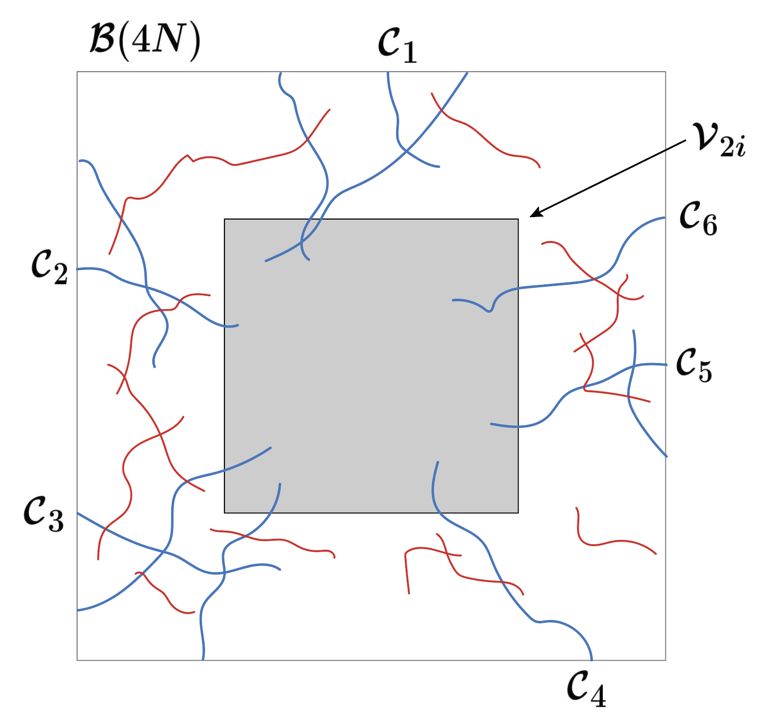
Figure 3. An example of $\mathfrak{U}_{i}$ : in this example, there are six clusters in $\mathfrak{C}$ , called $\mathcal{C}_{1},\mathcal{C}_{2},...,\mathcal{C}_{6}$ (colored in blue). The red lines represent the edge set $\mathcal{W}_{j}\setminus\mathcal{FI}^{u,T}$ . As shown in the picture, clusters $\mathcal{C}_{1}$ , $\mathcal{C}_{2}$ and $\mathcal{C}_{3}$ are connected by $\mathcal{W}_{j}$ , so they are contained in the same class of $\mathfrak{U}_{i}$ . In the same way, there are also two other classes in $\mathfrak{U}_{i}$ : $\left\{\mathcal{C}_{4}\right\}$ and $\left\{\mathcal{C}_{5},\mathcal{C}_{6}\right\}$ .

(9)

Recall the notation $\mu(\cdot)$ below (1.8). Let $n_{0}=\min\{n\mathrel{\mathop{\mathchar 58\relax}}L_{n}\geq\mu(10N)\}$ . Define the event

(5.22)

A\mathrel{\mathop{\mathchar 58\relax}}=\bigcap_{x\in\mathbb{Z}^{d}\mathrel{\mathop{\mathchar 58\relax}}B_{x}(L_{n_{0}})\subset B(4N)}\left\{B_{x}(L_{n_{0}})\xleftrightarrow{\mathcal{FI}^{u,T}}\partial B(6N)\right\}.

For the proof of Proposition 5.5, we need the following lemma similar to Lemma 4.2 in [10].

Lemma 5.6.

For any $\epsilon>0$ , there exists constant $c_{3}(\epsilon)>0$ such that for all $u\geq\widetilde{u}+2\epsilon$ , integers $N\geq 1$ , $a\in[4,N^{1/4}]$ and $0\leq i\leq\lceil\sqrt{N}\rceil-a$ ,

(5.23)

P\left[A\cap\{U_{i+a}>1\vee\frac{2U_{i}}{a}\}\right]\leq\exp(-c_3N^{1/4}).

Next we prove Proposition 5.5 given Lemma 5.6.

Proof of Proposition 5.5.

Fix $\epsilon>0$ and arbitrarily take $u\geq\widetilde{u}+2\epsilon$ . Note that

(5.24)

A^{c}\subset\bigcup_{y\in B(4N)}\left\{B_{y}(L_{n_{0}})\overset{\mathcal{FI}^{u,T}}{\nleftrightarrow}\partial B(6N)\right\}\subset\bigcup_{y\in B(4N)}\left\{B_{y}(\mu(10N))\overset{\mathcal{FI}^{u,T}}{\nleftrightarrow}\partial B_{y}(10N)\right\}.

By (5.24), we have

(5.25)

P\left[A^{c}\right]\leq(8N+1)^{d}\cdot P\left[B(\mu(10N))\overset{\mathcal{FI}^{u,T}}{\nleftrightarrow}\partial B(10N)\right].

Since $A\cap\{U_{\lfloor\sqrt{N}\rfloor}=1\}\subset\xi(N,u,u+\epsilon)$ , we have

(5.26)

\begin{split}P\left[\xi(N,u,u+\epsilon)^{c}\right]\leq&P\left[A^{c}\right]+P\left[A\cap\{U_{\lfloor\sqrt{N}\rfloor}>1\}\right].\end{split}

Note that there exists constant $C>0$ such that

(5.27)

|\mathfrak{C}|\leq|\partial B(4N)|\leq CN^{d-1}.

For an integer $a\in\left[4,N^{\frac{1}{4}}\right]$ , arbitrarily select an integer $M$ satifying $aM\leq\lceil\sqrt{N}\rceil$ and $\left(\frac{2}{a}\right)^{M}CN^{d-1}<1$ . If the event $\bigcap_{0\leq k<M}\left\{U_{(k+1)a}\leq 1\vee\frac{2U_{ka}}{a}\right\}$ happens, then either

(5.28)

U_{\lceil\sqrt{N}\rceil}\leq U_{Ma}\leq\frac{2}{a}U_{(M-1)a}\leq...\leq\left(\frac{2}{a}\right)^{M}U_{0}=\left(\frac{2}{a}\right)^{M}|\mathfrak{C}|\leq\left(\frac{2}{a}\right)^{M}CN^{d-1}<1,

or for some $0\leq k<M$ , $U_{(k+1)a}\leq 1$ and thus $U_{\lceil\sqrt{N}\rceil}\leq U_{(k+1)a}\leq 1$ .

Therefore, we have

(5.29)

\bigcap_{0\leq k<M}\left\{U_{(k+1)a}\leq 1\vee\frac{2U_{ka}}{a}\right\}\subset\left\{U_{\lceil\sqrt{N}\rceil}\leq 1\right\},

which implies that

(5.30)

A\cap\left\{U_{\lceil\sqrt{N}\rceil}>1\right\}\subset\bigcup_{0\leq k<M}\left\{A\cap\left\{U_{(k+1)a}>1\vee\frac{2U_{ka}}{a}\right\}\right\}.

By Lemma 5.6 and (5.30),

(5.31)

P\left[A\cap\left\{U_{\lceil\sqrt{N}\rceil}>1\right\}\right]\leq M\cdot P\left[A\cap\left\{U_{(k+1)a}>1\vee\frac{2U_{ka}}{a}\right\}\right]\leq M\cdot\exp(-c_3N^{1/4}).

Recall the definition of $\widetilde{u}$ in Section 1.1. Combining (5.25), (5.26), (5.31) and the fact that $\liminf\limits_{N\to\infty}(a_{N}+b_{N})\leq\limsup\limits_{N\to\infty}a_{N}+\liminf\limits_{N\to\infty}b_{N}$ , we conclude Proposition 5.5:

(5.32)

\begin{split}&\limsup\limits_{N\to\infty}\inf_{u\geq\widetilde{u}+2\epsilon}P\left[\xi(N,u,u+\epsilon)\right]\\ \geq&\limsup\limits_{N\to\infty}\left\{1-\sup_{u\geq\widetilde{u}+2\epsilon}P\left[A\cap\left\{U_{\lceil\sqrt{N}\rceil}>1\right\}\right]-\sup_{u\geq\widetilde{u}+2\epsilon}P\left[A^{c}\right]\right\}\\ \geq&1-\limsup_{N\to\infty}\left\{M\cdot\exp(-c_3N^{1/4})\right\}-\liminf_{N\to\infty}\left\{(8N+1)^{d}\cdot P\left[B(\mu(10N))\overset{\mathcal{FI}^{\widetilde{u}+2\epsilon,T}}{\nleftrightarrow}\partial B(10N)\right]\right\}\\ =&1.\end{split}

∎

Thus, in order to prove Proposition 5.5, it is sufficient to prove Lemma 5.6, where some additional notations need to be specified in advance:

(1)

For $0\leq i\leq\lceil\sqrt{N}\rceil$ , $k\in\{0,\frac{1}{2}\}$ and edge set $\mathcal{W}$ containing $\mathcal{FI}^{u,T}$ , let

(5.33)

\mathfrak{U}_{i+k,i+1}(\mathcal{W})\mathrel{\mathop{\mathchar 58\relax}}=\left\{class\ \mathscr{C}\in\mathfrak{U}_{i}(\mathcal{W})\mathrel{\mathop{\mathchar 58\relax}}\left(\cup\mathscr{C}\right)\cap\mathcal{V}_{2(i+1)}=\emptyset,\left(\cup\mathscr{C}\right)\cap\mathcal{V}_{2(i+k)}\neq\emptyset\right\},

(5.34)

U_{i,i+1}(\mathcal{W})\mathrel{\mathop{\mathchar 58\relax}}=|\mathfrak{U}_{i,i+1}(\mathcal{W})|.

(2)

Consider the following mapping $\psi_{i}\mathrel{\mathop{\mathchar 58\relax}}\mathfrak{U}_{i}(\mathcal{W})\setminus\mathfrak{U}_{i,i+1}(\mathcal{W})\to\mathfrak{U}_{i+1}(\mathcal{W})$ ,

(5.35)

\psi_{i}(\mathscr{C})=\mathscr{C}\setminus\{\mathcal{C}\in\mathscr{C}\mathrel{\mathop{\mathchar 58\relax}}\mathcal{C}\cap\mathcal{V}_{2(i+1)}=\emptyset\}.

Remark.

Note that $\psi_{i}$ is a bijection and thus

(5.36)

U_{i}(\mathcal{W})=U_{i+1}(\mathcal{W})+U_{i,i+1}(\mathcal{W}).

By (5.36), one has

(5.37)

U_{i+a}(\mathcal{W}_{i})+\sum_{j\mathrel{\mathop{\mathchar 58\relax}}i\leq j<i+a}U_{j,j+1}(\mathcal{W}_{i})=U_{i}(\mathcal{W}_{i})=U_{i}.

(3)

For $0\leq j<\lceil\sqrt{N}\rceil$ , define a set of equivalence classes $\widetilde{\mathfrak{U}}_{j}$ and an edge set $\mathcal{A}_{j}$ as follows: if $\mathfrak{U}_{j+\frac{1}{2},j+1}(\mathcal{W}_{j})=\emptyset$ , let $\mathcal{A}_{j}=\mathcal{V}_{2j+1}\setminus\mathcal{V}_{2j+2}$ and $\widetilde{\mathfrak{U}}_{j}=\mathfrak{U}_{j}(\mathcal{W}_{j})\setminus\mathfrak{U}_{j,j+1}(\mathcal{W}_{j})$ ; otherwise, define $\mathcal{A}_{j}=\mathcal{V}_{2j}\setminus\mathcal{V}_{2j+1}$ and $\widetilde{\mathfrak{U}}_{j}\mathrel{\mathop{\mathchar 58\relax}}=\mathfrak{U}_{j}(\mathcal{W}_{j})\setminus\mathfrak{U}_{j,j+1}(\mathcal{W}_{j})\cup\{\widetilde{\mathscr{C}}\}$ , where $\widetilde{\mathscr{C}}\mathrel{\mathop{\mathchar 58\relax}}=\{\mathcal{C}\mathrel{\mathop{\mathchar 58\relax}}there\ exists\ \mathscr{C}\in\mathfrak{U}_{j,j+1}(\mathcal{W}_{j})\ such\ that\ \mathcal{C}\in\mathscr{C}\}$ .

We hereby cite the following combinatorial lemma on $\widetilde{\mathfrak{U}}_{j}$ , which will play an important role in proving Lemma 5.6. The proof of this lemma can be totally found in the proof of Lemma 4.2 in [10].

Lemma 5.7.

For integers $0\leq j\leq\lceil\sqrt{N}\rceil$ and $4\leq a\leq\lfloor N^{\frac{1}{4}}\rfloor$ , given that the event $E_{j}\mathrel{\mathop{\mathchar 58\relax}}=A\cap\left\{U_{j+1}>1\vee\left(\frac{U_{j}}{a}+U_{j,j+1}(\mathcal{W}_{j})\right)\right\}$ happens, $\widetilde{\mathfrak{U}}_{j}$ has following properties with probability one:

(1)

for each $\mathscr{C}\in\widetilde{\mathfrak{U}}_{j}$ , $\cup\mathscr{C}$ crosses $\mathcal{A}_{j}$ and $\bigcup_{\mathscr{C}\in\widetilde{\mathfrak{U}}_{j}}\left(\cup\mathscr{C}\right)$ intersects all the boxes with radius $L_{n_{0}}$ contained in $V(\mathcal{A}_{j})$ ;
(2)

there exists a non-trivial partition $\widetilde{\mathfrak{U}}_{j}=\widetilde{\mathfrak{U}}_{j}^{1}\cup\widetilde{\mathfrak{U}}_{j}^{2}$ such that $1\leq|\widetilde{\mathfrak{U}}_{j}^{1}|\leq a$ and $\widetilde{\mathcal{C}}_{j}^{1}\overset{\mathcal{W}_{j+1}}{\not\leftrightarrow}\widetilde{\mathcal{C}}_{j}^{2}$ , where $\widetilde{\mathcal{C}}_{j}^{i}=\bigcup_{\mathscr{C}\in\widetilde{\mathfrak{U}}_{j}^{i}}\left(\cup\mathscr{C}\right)$ , $i\in\{1,2\}$ .

With Lemma 5.7, we are ready to conclude the proof of Lemma 5.6 and Proposition 5.5. See Figure 4 for an illustration of the main step in the proof of Lemma 5.6.

Proof of Lemma 5.6.

By (5.37), there must exist an integer $j\in\left[i,i+a\right)$ such that $U_{j,j+1}(\mathcal{W}_{j})\leq\frac{U_{i}}{a}$ . When the event in (5.23) occurs (we denote it by $E$ ), we have

(5.38)

U_{j}\geq U_{i+a}>\frac{2U_{i}}{a}=\frac{U_{i}}{a}+\frac{U_{i}}{a}\geq\frac{U_{j}}{a}+U_{j,j+1}(\mathcal{W}_{j}),

which implies that

(5.39)

E\subset\bigcup_{0\leq j<\lceil\sqrt{N}\rceil}E_{j}.

For any $0\leq j\leq\lceil\sqrt{N}\rceil$ , given the event $E_{j}$ , for any $\widetilde{\mathfrak{U}}_{j}^{0}$ , which is a possible realization of $\widetilde{\mathfrak{U}}_{j}^{0}$ , by Lemma 5.7 there exists a partition $\widetilde{\mathfrak{U}}_{j}^{0}=\widetilde{\mathfrak{U}}^{1,0}_{j}\cup\widetilde{\mathfrak{U}}_{j}^{2,0}$ such that $|\widetilde{\mathfrak{U}}^{1,0}_{j}|\leq a$ and $\widetilde{\mathcal{C}}_{j}^{1,0}\overset{\mathcal{W}_{j+1}}{\not\leftrightarrow}\widetilde{\mathcal{C}}_{j}^{2,0}$ , where $\widetilde{\mathcal{C}}_{j}^{i,0}=\bigcup_{\mathscr{C}\in\widetilde{\mathfrak{U}}_{j}^{i,0}}\left(\cup\mathscr{C}\right)$ , $i\in\{1,2\}$ .

Recall the definition of $n_{0}$ above (5.22) and the event $E_{j}$ in Lemma 5.7. We claim that given the event $E_{j}$ , there exist $k=\lfloor\frac{\sqrt{N}}{100\kappa L_{n_{0}}}\rfloor$ disjoint boxes $B_{x_{1}}(10\kappa L_{n_{0}})$ ,…, $B_{x_{k}}(10\kappa L_{n_{0}})$ contained in $V(\mathcal{A}_{j})$ with $x_{i}\in\mathbb{L}_{n_{0}}$ such that for all $1\leq l\leq k$ , $\widetilde{\mathcal{C}}_{j}^{1,0}$ and $\widetilde{\mathcal{C}}_{j}^{2,0}$ both intersect $B_{x_{l}}(8\kappa L_{n_{0}})$ . In fact, for $1\leq l\leq k$ , consider $T_{l}\mathrel{\mathop{\mathchar 58\relax}}=\left\{z\in\mathbb{Z}^{d}\mathrel{\mathop{\mathchar 58\relax}}|z|=b_{j}+50\kappa L_{n_{0}}+(l-1)80\kappa L{n_{0}}\right\}$ , where $b_{j}=\lfloor 4N-(2j+1)\sqrt{N}\rfloor$ if $\mathcal{A}_{j}=\mathcal{V}_{2j}\setminus\mathcal{V}_{2(j+1)}$ and $b_{j}=\lfloor 4N-(2j+2)\sqrt{N}\rfloor$ if $\mathcal{A}_{j}=\mathcal{V}_{2j+1}\setminus\mathcal{V}_{2(j+1)}$ . Note that for any $l_{1}\neq l_{2}$ and $y_{1}\in T_{l_{1}},y_{2}\in T_{l_{2}}$ , the boxes $B_{y_{1}}(20\kappa L_{n_{0}})$ and $B_{y_{2}}(20\kappa L_{n_{0}})$ are both contained in $V(\mathcal{A}_{j})$ and disjoint from each other. For any $x\in T_{l}$ , color it in black if $\widetilde{\mathcal{C}}_{1}^{0}$ intersects $B_{x}(L_{n_{0}})$ and in red if $\widetilde{\mathcal{C}}_{2}^{0}$ intersects $B_{x}(L_{n_{0}})$ . Note that for each $x\in T_{l}$ , $x$ must be colored for at least once (but possibly twice). Since both $\widetilde{\mathcal{C}}_{j}^{1,0}$ and $\widetilde{\mathcal{C}}_{j}^{2,0}$ cross $T_{l}$ , there must exist $x^{\prime}_{l},x^{\prime\prime}_{l}\in T_{l}$ such that $|x^{\prime}_{l}-x^{\prime\prime}_{l}|_{\infty}=1$ , and that $x^{\prime}_{l}$ , $x^{\prime\prime}_{l}$ are colored in black (or both black and red) and in red (or both black and red) respectively. Let $x_{l}$ be the closest vertex in $\mathbb{L}_{n_{0}}$ to $\frac{x^{\prime}+x^{\prime\prime}}{2}$ (if there are more than one such vertices, let $x_{l}$ be the lexicographically-smallest one of them). Then $\{B_{x_{l}}(10\kappa L_{n_{0}})\}_{1\leq l\leq k}$ are disjoint, and for all $1\leq l\leq k$ , both $\widetilde{\mathcal{C}}_{j}^{1,0}$ and $\widetilde{\mathcal{C}}_{j}^{2,0}$ intersect $B_{x_{l}}(8\kappa L_{n_{0}})$ . Hence,

(5.40)

\begin{split}P[E_{j}]\leq\sum_{\widetilde{\mathfrak{U}}_{j}^{0}}P\left[\widetilde{\mathfrak{U}}_{j}=\widetilde{\mathfrak{U}}_{j}^{0}\right]\cdot\sum_{\widetilde{\mathfrak{U}}_{j}^{1,0}\subset\widetilde{\mathfrak{U}}_{j}^{0}\mathrel{\mathop{\mathchar 58\relax}}|\widetilde{\mathfrak{U}}_{j}^{1,0}|\leq a}P\left[\bigcap\limits_{1\leq l\leq k}\{\widetilde{\mathcal{C}}_{j}^{1,0}\xleftrightarrow[B_{x_{l}}(10\kappa L_{n_{0}})]{\mathcal{FI}^{u+\epsilon,T}}\widetilde{\mathcal{C}}_{j}^{2,0}\}^{c}\bigg|\widetilde{\mathfrak{U}}_{j}=\widetilde{\mathfrak{U}}_{j}^{0}\right].\end{split}

For $i\in\{1,2\}$ , let $\mathcal{S}_{i}^{l}\mathrel{\mathop{\mathchar 58\relax}}=\mathcal{B}_{x_{l}}(10\kappa L_{n_{0}})\cap\left(\widetilde{\mathcal{C}}_{j}^{i,0}\cup\partial_{e}^{out}\widetilde{\mathcal{C}}_{j}^{i,0}\right)$ . When the event $\mathcal{S}_{1}^{l}\xleftrightarrow[B_{x_{l}}(10\kappa L_{n_{0}})]{\mathcal{FI}^{u+\epsilon,T}}\mathcal{S}_{2}^{l}$ occurs, there exists edge set $\{e^{l}_{1},e^{l}_{2}\}$ such that $e^{l}_{i}\in\partial_{e}^{out}\widetilde{\mathcal{C}}_{j}^{i,0}\cap\mathcal{B}_{x_{l}}(10\kappa L_{n_{0}})$ for $i\in\{1,2\}$ and $e_{1}^{l}\xleftrightarrow[B_{x_{l}}(10\kappa L_{n_{0}})]{\mathcal{FI}^{u+\epsilon,T}}e_{2}^{l}$ . We denote by $\{e^{l,0}_{1},e^{l,0}_{2}\}$ the lexicographically-smallest one among all edge sets $\{e^{l}_{1},e^{l}_{2}\}$ . Note that $\mathcal{A}_{j}\cap\left(\mathcal{B}(4N)\setminus\mathcal{V}_{2j}\right)=\emptyset$ and that the event $\widetilde{\mathfrak{U}}_{j}=\widetilde{\mathfrak{U}}_{j}^{0}$ only depends on

(5.41)

\sum_{(a_{i},\eta_{i})\in\mathcal{FI}^{T}}\delta_{\eta}\cdot\left(\mathbbm{1}_{0<a_{i}\leq u,\eta_{i}\cap\mathcal{B}(4N)\neq\emptyset}+\mathbbm{1}_{u<a_{i}\leq u+\epsilon,\eta_{i}\cap(\mathcal{B}(4N)\setminus\mathcal{V}_{2j})\neq\emptyset}\right),

which is independent to $\underline{\mathcal{FI}}^{\epsilon,T}_{1}\cap\mathcal{A}_{j}$ , where $\underline{\mathcal{FI}}^{\epsilon,T}_{1}\mathrel{\mathop{\mathchar 58\relax}}=\sum_{(a_{i},\eta_{i})\in\mathcal{FI}^{T}}\delta_{\eta}\cdot\mathbbm{1}_{u<a_{i}\leq u+\epsilon,|\eta_{i}|=1}$ .

By $\bigcap\limits_{i\in\{1,2\}}\{e^{l,0}_{i}\in\underline{\mathcal{FI}}^{\epsilon,T}_{1}\}\cap\left\{\mathcal{S}_{1}^{l}\xleftrightarrow[B_{x_{l}}(10\kappa L_{n_{0}})]{\mathcal{FI}^{u+\epsilon,T}}\mathcal{S}_{2}^{l}\right\}\subset\left\{\widetilde{\mathcal{C}}_{j}^{1,0}\xleftrightarrow[B_{x_{l}}(10\kappa L_{n_{0}})]{\mathcal{FI}^{u+\epsilon,T}}\widetilde{\mathcal{C}}_{j}^{2,0}\right\}$ , for any $1\leq l\leq k$ ,

(5.42)

\begin{split}&P\left[\{\widetilde{\mathcal{C}}_{j}^{1,0}\xleftrightarrow[B_{x_{l}}(10\kappa L_{n_{0}})]{\mathcal{FI}^{u+\epsilon,T}}\widetilde{\mathcal{C}}_{j}^{2,0}\}^{c}\bigg|\widetilde{\mathfrak{U}}_{j}=\widetilde{\mathfrak{U}}_{j}^{0},\bigcap_{1\leq m<l}\{\widetilde{\mathcal{C}}_{j}^{1,0}\xleftrightarrow[B_{x_{m}}(10\kappa L_{n_{0}})]{\mathcal{FI}^{u+\epsilon,T}}\widetilde{\mathcal{C}}_{j}^{2,0}\}^{c}\right]\\ \leq&P\left[\{\mathcal{S}_{1}^{l}\xleftrightarrow[B_{x_{l}}(10\kappa L_{n_{0}})]{\mathcal{FI}^{u+\epsilon,T}}\mathcal{S}_{2}^{l}\}^{c}\bigg|\widetilde{\mathfrak{U}}_{j}=\widetilde{\mathfrak{U}}_{j}^{0},\bigcap_{1\leq m<l}\{\widetilde{\mathcal{C}}_{j}^{1,0}\xleftrightarrow[B_{x_{m}}(10\kappa L_{n_{0}})]{\mathcal{FI}^{u+\epsilon,T}}\widetilde{\mathcal{C}}_{j}^{2,0}\}^{c}\right]\\ &+P\left[\mathcal{S}_{1}^{l}\xleftrightarrow[B_{x_{l}}(10\kappa L_{n_{0}})]{\mathcal{FI}^{u+\epsilon,T}}\mathcal{S}_{2}^{l}\bigg|\widetilde{\mathfrak{U}}_{j}=\widetilde{\mathfrak{U}}_{j}^{0},\bigcap_{1\leq m<l}\{\widetilde{\mathcal{C}}_{j}^{1,0}\xleftrightarrow[B_{x_{m}}(10\kappa L_{n_{0}})]{\mathcal{FI}^{u+\epsilon,T}}\widetilde{\mathcal{C}}_{j}^{2,0}\}^{c}\right]\\ &\ \ \ \cdot P\left[\bigcup\limits_{i=1,2}\{e^{l,0}_{i}\notin\underline{\mathcal{FI}}^{\epsilon,T}_{1}\}\bigg|\mathcal{S}_{1}^{l}\xleftrightarrow[B_{x_{l}}(10\kappa L_{n_{0}})]{\mathcal{FI}^{u+\epsilon,T}}\mathcal{S}_{2}^{l},\widetilde{\mathfrak{U}}_{j}=\widetilde{\mathfrak{U}}_{j}^{0},\bigcap_{1\leq m<l}\{\widetilde{\mathcal{C}}_{j}^{1,0}\xleftrightarrow[B_{x_{m}}(10\kappa L_{n_{0}})]{\mathcal{FI}^{u+\epsilon,T}}\widetilde{\mathcal{C}}_{j}^{2,0}\}^{c}\right]\\ =&1-c(\epsilon)\cdot P\left[\mathcal{S}_{1}^{l}\xleftrightarrow[B_{x_{l}}(10\kappa L_{n_{0}})]{\mathcal{FI}^{u+\epsilon,T}}\mathcal{S}_{2}^{l}\bigg|\widetilde{\mathfrak{U}}_{j}=\widetilde{\mathfrak{U}}_{j}^{0},\bigcap_{1\leq m<l}\{\widetilde{\mathcal{C}}_{j}^{1,0}\xleftrightarrow[B_{x_{m}}(10\kappa L_{n_{0}})]{\mathcal{FI}^{u+\epsilon,T}}\widetilde{\mathcal{C}}_{j}^{2,0}\}^{c}\right].\end{split}

We claim that for any $1\leq j\leq\lceil\sqrt{N}\rceil$ and $1\leq l\leq k$ , the event $\widetilde{\mathfrak{U}}_{j}=\widetilde{\mathfrak{U}}_{j}^{0}$ is measurable w.r.t. the following $\sigma$ -field:

(5.43)

\mathcal{F}_{l}\mathrel{\mathop{\mathchar 58\relax}}=\sigma\left(\sum_{(a_{i},\eta_{i})\in\mathcal{FI}^{T}}\delta_{(a_{i},\eta_{i})}\cdot\mathbbm{1}_{0<a_{i}\leq u+\epsilon,\eta\cap(\mathcal{S}_{1}^{l}\cup\mathcal{S}_{2}^{l}\cup\mathcal{B}^{c}_{x_{l}}(10\kappa L_{n_{0}}))\cap\mathcal{B}(4N)\neq\emptyset}\right).

Since $\widetilde{\mathfrak{U}}_{j}=\widetilde{\mathfrak{U}}_{j}^{0}$ is measurable w.r.t. $\sum_{(a_{i},\eta_{i})\in\mathcal{FI}}\delta_{(a_{i},\eta_{i})}\cdot\mathbbm{1}_{0<a_{i}\leq u+\epsilon,\eta\cap\mathcal{B}(4N)\neq\emptyset}$ , it is sufficient to confirm that $\widetilde{\mathfrak{U}}_{j}=\widetilde{\mathfrak{U}}_{j}^{0}$ is independent to $\sum_{(a_{i},\eta_{i})\in\mathcal{FI}}\delta_{(a_{i},\eta_{i})}\cdot\mathbbm{1}_{0<a_{i}\leq u+\epsilon,\eta\subset\mathcal{B}_{x_{l}}(10\kappa L_{n_{0}})\setminus(\mathcal{S}_{1}^{l}\cup\mathcal{S}_{2}^{l})}$ . For each given $\widetilde{\mathfrak{U}}_{j}^{0}$ , we enumerate the clusters in $\cup_{\mathscr{C}\in\widetilde{\mathfrak{U}}_{j}^{0}}\mathscr{C}$ by $\left\{\mathcal{C}_{1},...,\mathcal{C}_{n}\right\}$ . To ensure the event $\widetilde{\mathfrak{U}}_{j}=\widetilde{\mathfrak{U}}_{j}^{0}$ happens, it is sufficient to have that for any $1\leq i\leq n$ , $\left(\mathcal{C}_{i}\cup\partial_{e}^{out}\mathcal{C}\right)\cap\mathcal{FI}^{u,T}=\mathcal{C}_{i}$ and that $W_{j}$ , $W_{j+1}$ group $\left\{\mathcal{C}_{1},...,\mathcal{C}_{n}\right\}$ following the way given in $\widetilde{\mathfrak{U}}_{j}^{0}$ . Since each path in $\mathcal{FI}^{u+\epsilon,T}$ that totally contained in $\mathcal{B}_{x_{l}}(10\kappa L_{n_{0}})\setminus(\mathcal{S}_{1}^{l}\cup\mathcal{S}_{2}^{l})$ does not intersect any $\mathcal{C}_{i}$ , it will not have any impact on $\left(\mathcal{C}_{i}\cup\partial_{e}^{out}\mathcal{C}\right)\cap\mathcal{FI}^{u,T}$ and the way how $\left\{\mathcal{C}_{1},...,\mathcal{C}_{n}\right\}$ are grouped. In conclusion, $\widetilde{\mathfrak{U}}_{j}=\widetilde{\mathfrak{U}}_{j}^{0}$ is measurable w.r.t. $\mathcal{F}_{l}$ .

For each $1\leq l\leq k$ , noting that $\widetilde{\mathfrak{U}}_{j}=\widetilde{\mathfrak{U}}_{j}^{0}$ , $\bigcap_{1\leq m<l}\{\widetilde{\mathcal{C}}_{j}^{1,0}\xleftrightarrow[B_{x_{m}}(10\kappa L_{n_{0}})]{\mathcal{FI}^{u+\epsilon,T}}\widetilde{\mathcal{C}}_{j}^{2,0}\}^{c}$ are both measurable w.r.t. $\mathcal{F}_{l}$ , by Lemma 5.3 we have

(5.44)

\begin{split}P\left[\mathcal{S}_{1}^{l}\xleftrightarrow[B_{x_{l}}(10\kappa L_{n_{0}})]{\mathcal{FI}^{u+\epsilon,T}}\mathcal{S}_{2}^{l}\bigg|\widetilde{\mathfrak{U}}_{j}=\widetilde{\mathfrak{U}}_{j}^{0},\bigcap_{1\leq m<l}\{\widetilde{\mathcal{C}}_{j}^{1,0}\xleftrightarrow[B_{x_{m}}(10\kappa L_{n_{0}})]{\mathcal{FI}^{u+\epsilon,T}}\widetilde{\mathcal{C}}_{j}^{2,0}\}^{c}\right]\geq e^{-C_{4}(\log(L_{n_0}))^{2}}.\end{split}

Since $|\widetilde{\mathfrak{U}}_{j}^{0}|\leq CN^{d-1}$ , there are no more than $(CN^{d-1})^{a}$ subsets of $\widetilde{\mathfrak{U}}_{j}^{0}$ , whose cardinalities are not larger than $a$ . By (5.40), (5.42) and (5.44), we have

(5.45)

\begin{split}P[E_{j}]\leq&\sum_{\widetilde{\mathfrak{U}}_{j}^{0}}P\left[\widetilde{\mathfrak{U}}_{j}=\widetilde{\mathfrak{U}}_{j}^{0}\right]\sum_{\widetilde{\mathfrak{U}}_{j}^{1,0}\subset\widetilde{\mathfrak{U}}_{j}^{0}\mathrel{\mathop{\mathchar 58\relax}}|\widetilde{\mathfrak{U}}_{j}^{1,0}|\leq a}\prod_{l=1}^{k}P\bigg[\{\widetilde{\mathcal{C}}_{j}^{1,0}\xleftrightarrow[B_{x_{l}}(10\kappa L_{n_{0}})]{\mathcal{FI}^{u+\epsilon,T}}\widetilde{\mathcal{C}}_{j}^{2,0}\}^{c}\bigg|\widetilde{\mathfrak{U}}_{j}=\widetilde{\mathfrak{U}}_{j}^{0},\\ &\ \ \ \ \ \ \ \ \ \ \ \ \ \ \ \ \ \ \ \ \ \ \ \ \ \ \ \ \ \ \ \ \ \ \ \ \ \ \ \ \ \ \ \ \ \bigcap_{1\leq m<l}\{\widetilde{\mathcal{C}}_{j}^{1,0}\xleftrightarrow[B_{x_{m}}(10\kappa L_{n_{0}})]{\mathcal{FI}^{u+\epsilon,T}}\widetilde{\mathcal{C}}_{j}^{2,0}\}^{c}\bigg]\\ \leq&\sum_{\widetilde{\mathfrak{U}}^{0}_{j}}P\left[\widetilde{\mathfrak{U}}_{j}=\widetilde{\mathfrak{U}}_{j}^{0}\right]\cdot(CN^{d-1})^{a}\left[1-c\cdot e^{-C_{4}(\log(L_{n_0}))^{2}}\right]^{k}\\ =&(CN^{d-1})^{a}\left[1-c\cdot e^{-C_{4}(\log(L_{n_0}))^{2}}\right]^{k}.\end{split}

Recalling the definition of $n_{0}$ , we have $\mu(10N)\leq L_{n_{0}}\leq l_{0}\cdot\mu(10N)$ . Hence, one has $k\geq c^{\prime}\sqrt{N}/\mu(10N)$ and $1-e^{-C_{4}(\log(L_{n_0}))^{2}}\leq 1-e^{-C^{\prime}(\log(\mu(10N)))^{2}}$ .

Since $a\leq N^{1/4}$ and $\log(1-x)\leq-x$ ( $x>0$ ), we have: for each $c^{\prime}(\epsilon)>0$ , there exists integer $N_{0}(\epsilon)>0$ such that for all $N\geq N_{0}$ ,

(5.46)

\begin{split}P[E]\leq\sum_{j=0}^{\lceil\sqrt{N}\rceil}P[E_{j}]\leq&\lceil\sqrt{N}\rceil\cdot(CN^{d-1})^{a}\cdot\left[1-e^{-C_{4}(\log(L_{n_0}))^{2}}\right]^{k}\\ \leq&\lceil\sqrt{N}\rceil\cdot(CN^{d-1})^{N^{1/4}}\cdot\left[1-e^{-C^{\prime}(\log(\mu(10N)))^{2}}\right]^{c^{\prime}\sqrt{N}/\mu(10N)}\\ \leq&\exp(\log(N)+N^{1/4}\log(CN^{d-1})-\frac{c'\sqrt{N}}{\mu(10N)}\cdot e^{-C''(\log(10N))^{2/3}})\\ \leq&\exp(-c''N^{1/4}).\end{split}

From (5.46), we finally get (5.23). ∎

5.3. Renomalization

We define the following events: for $x\in\mathbb{L}_{0}$ , let

(5.47)

F^{(1)}_{x}=\left\{B_{x}(2L_{0}+1)\xleftrightarrow{\mathcal{FI}_{L_{0}}^{u-3\epsilon,T}}\partial B_{x}(6(2L_{0}+1))\right\},

(5.48)

\begin{split}F^{(2)}_{x}=\{&all\ clusters\ in\ \mathcal{FI}_{L_{0}}^{u-\frac{5\epsilon}{3},T}\cap\mathcal{B}_{x}(4(2L_{0}+1))\ crossing\ B_{x}(4(2L_{0}+1))\setminus B_{x}(2(2L_{0}+1))\\ &\ \ \ are\ connected\ by\ \mathcal{FI}_{L_{0}}^{u-\frac{4\epsilon}{3},T}\cap\mathcal{B}_{x}(4(2L_{0}+1))\},\end{split}

and

(5.49)

F_{0,x}\mathrel{\mathop{\mathchar 58\relax}}=F^{(1)}_{x}\cap F^{(2)}_{x}.

Fix a constant $\epsilon>0$ . For $x\in\mathbb{L}_{0}$ , we say that a box $B_{x}(L_{0})$ is $(u,L_{0})$ -good if the event $F_{0,x}$ occurs. Furthermore, we also say a cluster $A\subset\mathbb{Z}^{d}$ is a $(u,L_{0})$ -good cluster if $A$ is a union of some $(u,L_{0})$ -good boxes.

Similar to Proposition 4 in [10], we are to show that in a given box $B(N)$ , with a high probability there exists a sufficiently large $(u,L_{0})$ -good cluster intersecting all big connected subsets of $B(N)$ .

Proposition 5.8.

For any $\epsilon>0$ and $u\geq\widetilde{u}+6\epsilon$ , there exist $\rho(u,\epsilon)$ , $L_{0}(u,\epsilon)$ and $c_{4}(u,\epsilon)>0$ such that for all integers $N\geq 1$ ,

(5.50)

\begin{split}P[&there\ exists\ (u,L_{0})-good\ \ cluster\ J_{N}\subset B(2N)\ intersecting\ every\ cluster\ \\ &\ \ \mathcal{S}\subset\mathcal{B}(N)\ with\ diameter\geq N^{\frac{1}{2}}]\geq 1-\exp(-c_4N^\rho).\end{split}

Proof.

Recall the definition of the event $\xi(\cdot,\cdot,\cdot)$ in (5.19) and let $\xi_{x}\mathrel{\mathop{\mathchar 58\relax}}=x+\xi$ . Moreover, one may note that

(5.51)

\xi_{x}(2L_{0}+1,u-4\epsilon,u-3\epsilon)\cap\left\{\mathcal{B}_{x}(6(2L_{0}+1))\cap\left(\mathcal{FI}^{u-3\epsilon}-\mathcal{FI}_{L_{0}}^{u-3\epsilon}\right)=\emptyset\right\}\subset F^{(1)}_{x},

(5.52)

\xi_{x}(2L_{0}+1,u-\frac{14}{9}\epsilon,u-\frac{13}{9}\epsilon)\cap\left\{\mathcal{B}_{x}(6(2L_{0}+1))\cap\left(\mathcal{FI}^{u-\frac{13}{9}\epsilon}-\mathcal{FI}_{L_{0}}^{u-\frac{13}{9}\epsilon}\right)=\emptyset\right\}\subset F^{(2)}_{x}.

By (5.10), for any $u^{\prime}>0$ , we have

(5.53)

\begin{split}&P\left[\mathcal{B}_{x}(6(2L_{0}+1))\cap\left(\mathcal{FI}^{u^{\prime}}-\mathcal{FI}_{L_{0}}^{u^{\prime}}\right)\neq\emptyset\right]\leq C(u^{\prime})e^{-c(u^{\prime})L_{0}}.\end{split}

By (5.51), (5.52) and (5.53), for any $u\geq\widetilde{u}+6\epsilon$ and $x\in\mathbb{L}_{0}$ , we have

(5.54)

\begin{split}&P[F^{c}_{0,x}]\\ \leq&P\left[\xi^{c}_{x}\left(2L_{0}+1,u-\frac{14}{9}\epsilon,u-\frac{13}{9}\epsilon\right)\right]+P\left[\xi^{c}_{x}\left(2L_{0}+1,u-\frac{14}{9}\epsilon,u-\frac{13}{9}\epsilon\right)\right]+C(u)e^{-c(u)L_{0}}.\end{split}

Combine Proposition 5.5 and (5.54),

(5.55)

\limsup\limits_{L_{0}\to\infty}P[F_{0,x}]=1.

Note that it is sufficient to prove (5.50) in the case when $N\geq(L_{1})^{2}$ . Let $n=\max\{k\in\mathbb{N}\mathrel{\mathop{\mathchar 58\relax}}L_{k+1}\leq\sqrt{N}\}$ . Then we have

(5.56)

\frac{\sqrt{N}}{l_{0}^{2}}<L_{n}\leq\frac{\sqrt{N}}{l_{0}}.

For any $m\geq 0$ and a subset $A\subset\mathbb{L}_{m}$ , we say $A$ is $L_{m}$ -connected if the set of vertices $\{\frac{z}{2L_{m}+1}\mathrel{\mathop{\mathchar 58\relax}}z\in A\}$ is connected in $\mathbb{Z}^{d}$ .

For each $x\in\mathbb{L}_{n}$ , let $Comp(x)$ be the largest $L_{0}$ -connected component (in the sense of diameter) consisting of vertices $y\in\mathbb{L}_{0}\cap B_{x}(4\kappa L_{n})$ such that the event $F_{0,y}$ happens (if there are more than one “largest clusters”, let $Comp(x)$ be the lexicographically-smallest one of them). Define the following $(u,L_{0})$ -good cluster:

(5.57)

J_{N}=\bigcup_{x\in\mathbb{L}_{n}\cap B(N)}\bigcup_{y\in Comp(x)}B_{y}(L_{0}).

Note that $J_{N}\subset B(N+4\kappa L_{n}+L_{0})\subset B(2N)$ .

Recall the event $\mathscr{G}_{n}^{0}$ in (5.1) and define $\mathscr{G}_{n,x}^{0}=x+\mathscr{G}_{n}^{0}$ . Let $G_{N}=\bigcap_{x\in\mathbb{L}_{n}\cap B(N)}\mathscr{G}_{n,x}^{0}$ . Then we try to confirm that when $G_{N}$ happens, $J_{N}$ satisfies the condition in (5.50):

We first check that given the event $G_{N}$ , $J_{N}$ is $L_{0}$ -connected: for any $x,y\in\mathbb{L}_{n}\cap B(N)$ such that $|x-y|_{1}=2L_{n}+1$ , since each pair of oppsite faces of $B_{x}(\kappa L_{n})$ are both subsets of $B_{x}(10\kappa L_{n})$ with diameters larger than $\kappa L_{n}$ (in other words, they are both $0$ -admissible), there must exist a $0$ -bridge $\mathfrak{B}^{0}$ with $(u,L_{0})$ -boxes connecting both of the two opposite faces. Since the diameter of $\{z\mathrel{\mathop{\mathchar 58\relax}}B_{z}(L_{0})\in\mathfrak{B}^{0}\}$ must be larger than $\kappa L_{n}$ and $Comp(x)$ is the largest, we have that $\mathcal{S}_{x}\mathrel{\mathop{\mathchar 58\relax}}=\bigcup_{z\in Comp(x)}\mathcal{B}_{z}(L_{0})$ is $0$ -admissible in both $\mathcal{B}_{x}(10\kappa L_{n})$ and $\mathcal{B}_{y}(10\kappa L_{n})$ . In the same way, $\mathcal{S}_{y}$ is $0$ -admissible in both $\mathcal{B}_{x}(10\kappa L_{n})$ and $\mathcal{B}_{y}(10\kappa L_{n})$ as well. By the definition of $G_{N}$ , we have that

(5.58)

\mathcal{S}_{x}\cap\mathcal{S}_{y}\neq\emptyset,

which implies that $J_{N}$ is connected.

Meanwhile, for any connected subset $\mathcal{S}\subset\mathcal{B}(N)$ with diameter at least $\sqrt{N}$ , we have $\text{diam}(S)\geq\sqrt{N}\geq 10\kappa L_{n}$ . Arbitrarily choose a vertex $x\in\mathbb{L}_{n}\cap B(N)$ such that $\mathcal{S}\cap\mathcal{B}_{x}(L_{n})\neq\emptyset$ . Then $\mathcal{S}\cap\mathcal{B}_{x}(4\kappa L_{n})$ contains a cluster with diameter at least $\kappa L_{n}$ . Sicne the event $G_{N}$ occurs, there must exist a $0$ -bridge $\mathfrak{B}^{0}$ with $(u,L_{0})$ -boxes intersctig both $\mathcal{S}$ and $\mathcal{S}_{x}$ . Therefore, we have that $\mathcal{S}\cap\mathcal{S}_{x}\neq\emptyset$ . In conclusion, if we denote the event in (5.50) by $D$ , then

(5.59)

P\left[D\right]\geq P[G_{N}].

Note that there exists a large enough $L_{0}$ such that events $\{F_{0,x}\}_{x\in\mathbb{L}_{0}}$ defined in (5.49) satisfy all the conditions in Lemma 5.1. In fact, since $F_{0,x}$ only depends on $\sum_{\eta\in\mathcal{FI}^{u,T}_{L_{0}}}\delta_{\eta}\cdot\mathbbm{1}_{\eta(0)\in B_{x}(20L_{0})}$ and $\kappa\geq 100$ , the first condition for $F_{0,x}$ in Lemma 5.1 holds; meanwhile, by (5.55), we can choose a sufficient large $L_{0}$ such that $P[F_{0,x}]\leq c_{1}$ for all $x\in\mathbb{L}_{0}$ .

By (5.55) and Lemma 5.1, there exists a sufficient large $L_{0}$ such that

(5.60)

P\left[D\right]\geq P[G_{N}]\geq 1-2^{-2^{n}}=1-\exp(-c'N^\rho).

∎

5.4. Proving SQ3

With Proposition 5.8, we are ready to hereby finish the proof of SQ3.

We first note that it suffices to prove that for any $u>\widetilde{u}$ , there exists $c(u)>0$ , $\rho(u)>0$ such that for all integer $N\geq 1$ ,

(5.61)

P\left[\text{Exist}(N,\mathcal{FI}^{u,T})^{c}\right]\leq\exp(-cN^\rho),

(5.62)

P\left[\text{Unique}(N,\mathcal{FI}^{u,T})^{c}\right]\leq\exp(-cN^\rho).

For any $u>\widetilde{u}$ , let $\epsilon\mathrel{\mathop{\mathchar 58\relax}}=\frac{u-\widetilde{u}}{10}$ . By defintion we have $u\geq\widetilde{u}+6\epsilon$ .

For the first part, when the event in (5.50) occurs, there exists at least one $(u,L_{0})$ -good cluster satisfying the condition of $J_{N}$ in (5.50). We denote the lexicographically-smallest one of them by $J_{N}^{0}$ . Note that $\text{diam}(J_{N}^{0})\geq 2N-2\sqrt{N}$ . Recalling the definition of “ $(u,L_{0})$ -good” below (5.49), there exists a connected cluster $\mathcal{J}_{N}^{0}\subset\mathcal{FI}^{u-\epsilon,T}$ intersecting every $(u,L_{0})$ -box in $J_{N}^{0}$ . Therefore, (5.61) holds by Proposition 5.8.

For the second part, we denote the event in (5.50) by $A$ . For any $x\in B(N)$ , let $\mathcal{C}(x)$ be the connected cluster in $\mathcal{FI}^{u,T}\cap\mathcal{B}(N)$ containing $x$ (if such cluster does not exist, set $\mathcal{C}(x)\mathrel{\mathop{\mathchar 58\relax}}=\emptyset$ ).

If $\text{Unique}(N,\mathcal{FI}^{u,T})$ does not happen, there must exist two clusters $\mathcal{L}_{1}$ and $\mathcal{L}_{2}$ with diameters $\geq\frac{R}{10}$ in $\mathcal{FI}^{u,T}\cap\mathcal{B}(N)$ , which are not connected within $\mathcal{FI}^{u,T}\cap\mathcal{B}(2N)$ . Since $\mathcal{J}_{N}^{0}\subset\mathcal{FI}^{u-\epsilon,T}$ , there must exist one cluster in $\{\mathcal{L}_{1},\mathcal{L}_{2}\}$ such that $V(\mathcal{L}_{i})\cap V(\mathcal{J}_{N}^{0})=\emptyset$ . By Proposition 5.8,

(5.63)

\begin{split}&P\left[\text{Unique}(N,\mathcal{FI}^{u,T})^{c}\right]\\ \leq&P\left[A^{c}\right]+P\left[\text{Unique}(N,\mathcal{FI}^{u,T})^{c}\cap A\right]\\ \leq&\exp(-cN^\rho)+P\left[\text{Unique}(N,\mathcal{FI}^{u,T})^{c}\cap A\right]\\ \leq&\exp(-cN^\rho)+\sum_{x\in B(N)}P\left[A,\text{diam}(\mathcal{C}(x))\geq N/10,V(\mathcal{C}(x))\cap V(\mathcal{J}_{N}^{0})=\emptyset\right].\end{split}

It is sufficient to prove: there exist $c^{\prime}(u),\rho^{\prime}(u)>0$ such that for any $N\geq 1$ and $x\in B(N)$ ,

(5.64)

P\left[A,\text{diam}(\mathcal{C}(x))\geq N/10,V(\mathcal{C}(x))\cap V(\mathcal{J}_{N}^{0})=\emptyset\right]\leq\exp(-c'N^{\rho'}).

For any $L\in\mathbb{N}^{+}$ , consider the following point measure

(5.65)

\underline{\mathcal{FI}}^{\epsilon,T}_{L}\mathrel{\mathop{\mathchar 58\relax}}=\sum_{(a_{n},\eta_{n})\in\mathcal{FI}^{T}}\delta_{\eta_{n}}\cdot\mathbbm{1}_{u-\epsilon<a_{n}\leq u,|\eta_{n}|=L}

and the $\sigma$ -filed $\mathcal{F}\mathrel{\mathop{\mathchar 58\relax}}=\sigma\left(\left(\mathcal{FI}^{u,T}-\underline{\mathcal{FI}}^{\epsilon,T}_{1}\right)\cap\mathcal{B}(2N)\right)$ . Note that $\underline{\mathcal{FI}}^{\epsilon,T}_{1}$ has the same distribution as a Bernoulli bond percolation. We denote the law of $\underline{\mathcal{FI}}^{\epsilon,T}_{1}$ by $P_{1}$ .

Since the event $A$ is measurable w.r.t. $\mathcal{F}$ , we have

(5.66)

\begin{split}&P\left[A,\text{diam}(\mathcal{C}(x))\geq N/10,V(\mathcal{C}(x))\cap V(\mathcal{J}_{N}^{0})=\emptyset\right]\\ =&E\left[\mathbbm{1}_{A}\cdot P_{1}\left[\text{diam}(\mathcal{C}(x))\geq N/10,V(\mathcal{C}(x))\cap V(\mathcal{J}_{N}^{0})=\emptyset\big|\mathcal{F}\right]\right].\end{split}

For each $x\in B(N)$ , denote the connected component in $(\mathcal{FI}^{u,T}-\underline{\mathcal{FI}}^{\epsilon,T}_{1})\cap\mathcal{B}(2N)$ containing $x$ by $\widetilde{\mathcal{C}}(x)$ (we also set $\widetilde{\mathcal{C}}(x)=\emptyset$ if there is no such a cluster). Note that conditioned on $\mathcal{F}$ , the edge sets $J_{N}^{0}$ , $\mathcal{J}^{0}_{N}$ and $\widetilde{\mathcal{C}}(x)$ are all deterministic.

For $x\in B(N)$ , similar to the proof of Proposition 1.5 in [10], we run a random algorithm $\mathfrak{T}_{x}$ under the following laws:

(1)

Initially, set $\widetilde{\mathcal{C}}_{0}(x)\mathrel{\mathop{\mathchar 58\relax}}=\widetilde{\mathcal{C}}(x)$ , $\text{Open}_{0}=\emptyset$ , $\text{Close}_{0}\mathrel{\mathop{\mathchar 58\relax}}=\emptyset$ and $D_{0}\mathrel{\mathop{\mathchar 58\relax}}=J_{N}^{0}$ .
(2)
For step $i$ , we already have $\widetilde{\mathcal{C}}_{i}(x)$ , $\text{Open}_{i}$ , $\text{Close}_{i}$ and $\mathcal{D}_{i}$ . If $\partial_{e}^{out}\widetilde{\mathcal{C}}_{i}(x)\setminus\text{Close}_{i}\subset\partial_{e}^{out}\mathcal{B}(2N)$ or $\widetilde{\mathcal{C}}_{i}(x)$ intersects $V(\mathcal{J}_{N}^{0})$ , stop the process. Otherwise, we denote the lexicographically-smallest edge in $\partial_{e}^{out}\widetilde{\mathcal{C}}_{i}(x)$ by $e_{i+1}$ .
1. (a)
  
  If $e_{i+1}\in\underline{\mathcal{FI}}^{\epsilon,T}_{1}$ and $e_{i+1}$ does not interset $D_{i}$ , let $\text{Open}_{i+1}=\text{Open}_{i}\cup\{e_{i+1}\}$ , $\text{Close}_{i+1}=\text{Close}_{i}$ , $D_{i+1}=D_{i}$ and let $\widetilde{\mathcal{C}}_{i+1}(x)$ the connected cluster in $[(\mathcal{FI}^{u,T}-\underline{\mathcal{FI}}^{\epsilon,T}_{1})\cap\mathcal{B}(2N)]\cup\text{Open}_{i+1}$ containing $x$ ;
2. (b)
  
  If $e_{i+1}\in\underline{\mathcal{FI}}^{\epsilon,T}_{1}$ and $e_{i+1}$ intersets $D_{i}$ at the boundary of a $0$ -vertex-box $B_{x_{i+1}}(L_{0})$ , sample the configuration of $\underline{\mathcal{FI}}^{\epsilon,T}_{1}\cap\mathcal{B}_{x_{i+1}}(L_{0})\setminus\left(\text{Open}_{i}\cup\text{Close}_{i}\right)$ . Then denote the sets of open and closed edges in it by $\mathcal{OP}_{i+1}$ and $\mathcal{CL}_{i+1}$ respectively. Let $\text{Open}_{i+1}=\text{Open}_{i}\cup\mathcal{OP}_{i+1}$ , $\text{Close}_{i+1}=\text{Close}_{i}\cup\mathcal{CL}_{i+1}$ , $D_{i+1}=D_{i}\setminus B_{x_{i+1}}(L_{0})$ and let $\widetilde{\mathcal{C}}_{i+1}(x)$ be the connected cluster in $[(\mathcal{FI}^{u,T}-\underline{\mathcal{FI}}^{\epsilon,T}_{1})\cap\mathcal{B}(2N)]\cup\text{Open}_{i+1}$ containing $x$ ;
3. (c)
  
  If $e_{i+1}\notin\underline{\mathcal{FI}}^{\epsilon,T}_{1}$ , let $\widetilde{\mathcal{C}}_{i+1}(x)=\widetilde{\mathcal{C}}_{i}(x)$ , $\text{Open}_{i+1}=\text{Open}_{i}$ , $D_{i+1}=D_{i}$ and $\text{Close}_{i+1}=\text{Close}_{i}\cup\{e_{i+1}\}$ .

Given configuration of $\mathcal{F}$ , we denote by $N_{1}$ the number of steps that the condition in (b) holds before the random algorithm terminates. When event $A$ and $V(\mathcal{C}(x))\cap V(\mathcal{J}_{N}^{0})=\emptyset$ happen, by property of $J_{N}^{0}$ (see (5.50)), we have

(5.67)

\text{diam}(\mathcal{C}(x))\leq 10\sqrt{N}\cdot N_{1}.

Therefore, on the event $A$ , we have

(5.68)

\begin{split}&P_{1}\left[\text{diam}(\mathcal{C}(x))\geq N/10,V(\mathcal{C}(x))\cap V(\mathcal{J}_{N}^{0})=\emptyset\big|\mathcal{F}\right]\\ \leq&P_{1}\left[N_{1}\geq\lfloor\frac{\sqrt{N}}{100}\rfloor,V(\mathcal{C}(x))\cap V(\mathcal{J}_{N}^{0})=\emptyset\bigg|\mathcal{F}\right].\end{split}

Note that all the $0$ -vertex-boxes $B_{x_{i+1}}(L_{0})$ (recall step (b) in the random algorithm $\mathfrak{T}_{x}$ ) are disjoint to each other by definition of $D_{i}$ . Each time when the condition in (b) holds, $\widetilde{\mathcal{C}}_{i+1}(x)$ will intersect $\mathcal{J}_{N}^{0}$ with at least $c^{\prime\prime}(L_{0},\epsilon)\in(0,1)$ probability (if $\mathcal{B}_{x_{i}}(2L_{0}+1)\subset\underline{\mathcal{FI}}^{\epsilon,T}_{1}$ , then $\widetilde{\mathcal{C}}_{i+1}(x)\cap\mathcal{J}_{N}^{0}\neq\emptyset$ ). Hence,

(5.69)

P_{1}\left[N_{1}\geq\lfloor\frac{\sqrt{N}}{100}\rfloor,V(\mathcal{C}(x))\cap V(\mathcal{J}_{N}^{0})=\emptyset\bigg|\mathcal{F}\right]\leq(1-c^{\prime\prime})^{\lfloor\frac{\sqrt{N}}{100}\rfloor}.

By (5.63), (5.64), (5.66), (5.68) and (5.69), we get (5.62) and finish the proof of SQ3. ∎

6. Proof of SQ4

In this section, we will first prove the equality of critical values for restricted model $\mathcal{FI}^{u,T}_{L}$ . And then we will prove an important inequality to estimate the influence of remaining part $\mathcal{FI}^{u,T}-\mathcal{FI}^{u,T}_{L}$ on the probability of an crossing event. Applying these two results, we finally conclude SQ4 by contradiction.

Like in Section 5, we also fix $d\geq 3$ and $T>0$ in this section.

6.1. Equality for Critical Values of $\mathcal{FI}_{L}^{u,T}$

We hereby recall the definition of $\mathcal{FI}_{L}^{u,T}$ and define critical values of this restricted system,

(1)

$u_{*}^{L}=\sup\left\{u>0\mathrel{\mathop{\mathchar 58\relax}}P\left[0\xleftrightarrow{\mathcal{FI}_{L}^{u,T}}\infty\right]=0\right\}$ ;
(2)

$u_{**}^{L}=\sup\left\{u>0\mathrel{\mathop{\mathchar 58\relax}}\inf\limits_{R\in\mathbb{N}^{+}}P\left[B(R)\xleftrightarrow{\mathcal{FI}_{L}^{u,T}}\partial B(2R)\right]=0\right\}$ ;
(3)

$\widetilde{u}^{L}=\inf\left\{u>0\mathrel{\mathop{\mathchar 58\relax}}\inf\limits_{R\in\mathbb{N}}R^{d}P\left[B(\mu(R))\stackrel{{\scriptstyle\mathcal{FI}_{L}^{u,T}}}{{\nleftrightarrow}}\partial B(R)\right]=0\right\}$ , where $\mu(R)=\lfloor e^{(\log(R))^{1/3}}\rfloor$ .

Like Proposition 1.3 in [10], we show that these critical values are equivalent to each other.

Proposition 6.1.

For any $L\in\mathbb{N}^{+}$ , $u_{*}^{L}=u_{**}^{L}=\widetilde{u}^{L}$ .

Before proving Proposition 6.1, we first state several basic properties of $\mathcal{FI}_{L}^{u,T}$ .

Lemma 6.2.

$\mathcal{FI}_{L}^{u,T}$ has the following properties:

(a)

Lattice Symmetry: Assume that $\phi$ is either a shift, reflection w.r.t. hyperplanes spanned by the base vectors or rotation by $\frac{k\pi}{2}$ ( $k\in\mathbb{Z}$ ) of $\mathbb{Z}^{d}$ . Then $\phi(\mathcal{FI}_{L}^{u,T})$ has the same distribution as $\mathcal{FI}_{L}^{u,T}$ .

(b)

Positive Association: The FKG inequality holds. I.e., if $f$ and $g$ are both increasing functions (or both decreasing functions) on $\{0,1\}^{\mathbb{L}^{d}}$ such that $E[f^{2}],E[g^{2}]<\infty$ , then

(6.1)

E\left[f(\mathcal{FI}_{L}^{u,T})g(\mathcal{FI}_{L}^{u,T})\right]\geq E\left[f(\mathcal{FI}_{L}^{u,T})\right]E\left[g(\mathcal{FI}_{L}^{u,T})\right].

(c)

Uniform Finite-energy: For any $u>0$ , there exists $c_{UF}(u)\in(0,1)$ such that for any edge set $\mathcal{K}$ , event $E\in\sigma\left(\mathcal{K}\cap\mathcal{FI}_{L}^{u,T}\right)$ and edge $e\in\mathbb{L}^{d}\setminus\mathcal{K}$ ,

(6.2) $1-c_{UF}\leq P\left[e\notin\mathcal{FI}_{L}^{u,T}\big|E\right]\leq c_{UF}.$
(d)

Bounded-range i.i.d. Coding: For $x\in\mathbb{Z}^{d}$ and $L\in\mathbb{N}^{+}$ , denote

(6.3) $\mathcal{FI}_{L}^{u,T}(x)=\sum_{\eta\in\mathcal{FI}^{u,T}}\delta_{\eta}\cdot\mathbbm{1}_{\eta(0)=x,|\eta|\leq L}.$

Then for any $e\in\mathbb{L}^{d}$ , $\mathbbm{1}_{e\in\mathcal{FI}_{L}^{u,T}}$ only depends on $\left\{\mathcal{FI}_{L}^{u,T}(x)\mathrel{\mathop{\mathchar 58\relax}}d_{1}(x,e)\leq L-1\right\}$ .
(e)

Sprikling Property: For any $u>u^{\prime}\geq 0$ , there exists $\epsilon>0$ s.t. $\mathcal{FI}^{u,T}_{L}$ stochastically dominates $\mathcal{FI}^{u^{\prime},T}_{L}\cup\zeta_{\epsilon}$ , where $\zeta_{\epsilon}$ is a Bernoulli bond percolation on $\mathbb{L}^{d}$ with parameter $\epsilon$ .
(f)

Uniform Embeddability: For any $u>0$ , there exists $c_{UE}(u)>0$ such that for any $e\in\mathbb{L}^{d}$ , subset $K\subsetneqq\{z\in\mathbb{Z}^{d}\mathrel{\mathop{\mathchar 58\relax}}d(e,\{z\})\leq L-1\}$ and configuration $\omega$ of $\left\{\mathcal{FI}_{L}^{u,T}(x)\mathrel{\mathop{\mathchar 58\relax}}x\in K\right\}$ ,

(6.4) $P[e\in\mathcal{FI}_{L}^{u,T}|\omega]>c_{UE}.$

Proof of Lemma 6.2.

Property (a) and (d) are immediate. For property (b), see Proposition A.3. Since $\mathcal{FI}_{1}^{u-u^{\prime}}$ has the same distribution as a Bernoulli bond percolation, property (e) also holds. Hence, it is sufficient to check property (c) and (f).

First consider the first inequality of (6.2). Note that events $E$ and $\{e=\{x,y\}\notin\mathcal{FI}_{L}^{u,T}\}$ are both measurable w.r.t. $\mathscr{A}\mathrel{\mathop{\mathchar 58\relax}}=\sum_{(u_{i},\eta_{i})\in\mathcal{FI}}\delta_{\eta_{i}}\cdot\mathbbm{1}_{0<u_{i}\leq u,\eta_{i}\cap(\mathcal{K}\cap\{e\})\neq\emptyset}$ . For any configuration $\omega$ of $\mathscr{A}$ such that the event $E\cap\{e=\{x,y\}\notin\mathcal{FI}_{L}^{u,T}\}$ happens, there exists no path $\eta$ in $\mathcal{FI}_{L}^{u,T}$ such that $\eta(0)=x$ and $\eta(1)=y$ . Thus, let $\eta_{0}=(x,y)$ , then the configuration $\omega+\delta_{\eta_{0}}\in E\cap\{e\in\mathcal{FI}_{L}^{u,T}\}$ . Note that for $N_{u,T}\sim\text{Pois}(\frac{2du}{T+1})$ ,

(6.5)

\frac{P[\omega]}{P[\omega+\delta_{\eta_{0}}]}=\frac{P[N_{u,T}=0]}{P[N_{u,T}=1]\cdot P_{x}^{(T)}(\eta_{0})}\mathrel{\mathop{\mathchar 58\relax}}=c\in(0,1).

By (6.5), we have

(6.6)

P[E\cap\{e=\{x,y\}\notin\mathcal{FI}_{L}^{u,T}\}]\leq c\cdot P[E\cap\{e=\{x,y\}\in\mathcal{FI}_{L}^{u,T}\}],

which implies

(6.7)

P[\{e=\{x,y\}\notin\mathcal{FI}_{L}^{u,T}\}|E]\leq\frac{c}{1+c}<1.

Now consider the second inequality of (6.2). For $\mathcal{K}\subset\mathbb{L}^{d}$ and $e=\{x,y\}$ , denote that

(6.8)

K_{0}=\left\{z\in\mathbb{Z}^{d}\mathrel{\mathop{\mathchar 58\relax}}d_{1}(z,\mathcal{K})\leq L-1,d_{1}(z,e)\leq L-1\right\}.

For any $z\in\mathbb{Z}^{d}$ , since the number of paths with starting point $z$ and length $\leq L$ is finite, the number of $\omega$ , configurations of $\{\mathcal{FI}_{L}^{u,T}(z)\mathrel{\mathop{\mathchar 58\relax}}z\in K_{0}\}$ , such that for any $\eta_{1},\eta_{2}\in\omega,\eta_{1}\neq\eta_{2}$ is also finite. We can define

(6.9)

c^{\prime}\mathrel{\mathop{\mathchar 58\relax}}=\min_{\begin{subarray}{c}\omega\mathrel{\mathop{\mathchar 58\relax}}\text{configuration of}\ \{\mathcal{FI}_{L}^{u,T}(z)\mathrel{\mathop{\mathchar 58\relax}}z\in K_{0}\}\\ \text{such that for any}\ \eta_{1},\eta_{2}\in\omega,\ \eta_{1}\neq\eta_{2}\end{subarray}}P[\omega]\in(0,1).

We introduce four mappings, $\phi_{1}$ , $\phi_{2}$ , $\phi_{3}$ and $\phi$ as follows:

$\phi_{1}$ :

for any path $\eta=(\eta(0),...,\eta(n))\in W^{\left[0,\infty\right)}$ , if $\eta$ does not intersect $K_{0}$ , define $\phi_{1}(\eta)=\emptyset$ ; otherwise, let $m_{0}\mathrel{\mathop{\mathchar 58\relax}}=\inf\left\{0\leq i\leq n\mathrel{\mathop{\mathchar 58\relax}}\eta(i)\in K_{0}\right\}$ and then define $\phi_{1}(\eta)=(\eta(m_{0}),...,\eta(n))$ ;

\phi_{2}

for any path $\eta=(\eta(0),...,\eta(n))\in W^{\left[0,\infty\right)}$ , if $\eta\cap e=\emptyset$ , define $\phi_{2}(\eta)=\{\eta\}$ ; otherwise, we denote all integers $i$ such that $\{\eta(i),\eta(i+1)\}=e$ by $\{i_{1},...,i_{k}\}$ , where $0\leq i_{1}\leq...\leq i_{k}\leq n-1$ , and then define

(6.10)

\begin{split}\phi_{2}(\eta)=&\left\{(\eta(i_{j}+1),...,\eta(i_{j+1}))\mathrel{\mathop{\mathchar 58\relax}}1\leq j\leq k-1\right\}\\ &\cup\left\{(\eta(0),...,\eta(i_{1})),(\eta(i_{k}+1),...,\eta(n))\right\}.\end{split}

$\phi_{3}$ :

for any point measure $\omega$ on $W^{\left[0,\infty\right)}$ containing finitely many paths, we denote all the diffierent paths in $\omega$ by $\{\eta_{1},...,\eta_{n}\}$ . Then we define $\phi_{3}(\omega)=\sum_{i=1}^{n}\delta_{\eta_{i}}$ .

\phi

for any point measure $\omega$ on $W^{\left[0,\infty\right)}$ containing finitely many paths, we also define that

(6.11)

\phi(\omega)\mathrel{\mathop{\mathchar 58\relax}}=\phi_{3}\left(\sum_{\eta\in\omega}\sum_{\zeta\in\phi_{2}(\eta)}\delta_{\phi_{1}(\zeta)}\right).

We claim that for any configuration $\omega$ of $\{\mathcal{FI}_{L}^{u,T}(z)\mathrel{\mathop{\mathchar 58\relax}}z\in K_{0}\}$ , $\phi(\omega)$ must be one of the configurations mentioned in (6.9) and satisfies $\phi(\omega)\cap\mathcal{K}=\omega\cap\mathcal{K}$ . In fact, for each path in $\omega$ , the mapping $\phi_{2}$ will cut off all steps traversing the edge $e$ while still visits exactly the same set of edges. Then for each sub-path, the mapping $\phi_{1}$ only keep the part of it after first intersecting $K_{0}$ . Thus, compared with $\omega$ , $\sum_{\eta\in\omega}\sum_{\zeta\in\phi_{2}(\eta)}\delta_{\phi_{1}(\zeta)}$ does not traverse $e$ and visits the same edges in $\mathcal{K}$ as $\omega$ does. Finally, the mapping $\phi_{3}$ eliminates those repetitive paths in $\sum_{\eta\in\omega}\sum_{\zeta\in\phi_{2}(\eta)}\delta_{\phi_{1}(\zeta)}$ and maps it to one of the configurations in (6.9).

Let $K_{1}\mathrel{\mathop{\mathchar 58\relax}}=\left\{z\in\mathbb{Z}^{d}\mathrel{\mathop{\mathchar 58\relax}}d(z,\mathcal{K})\leq L-1\right\}$ and note that $K_{0}\subsetneqq K_{1}$ . For any configuration $\omega^{1}$ of $\{\mathcal{FI}_{L}^{u,T}(z)\mathrel{\mathop{\mathchar 58\relax}}z\in K_{1}\}$ , let $\omega^{1}_{|K_{0}}=\sum_{\eta\in\omega^{1}}\delta_{\eta}\cdot\mathbbm{1}_{\eta(0)\in K_{0}}$ and $\widetilde{\omega}^{1}=\sum_{\eta\in\omega^{1}}\delta_{\eta}\cdot\mathbbm{1}_{\eta(0)\in K_{1}\setminus K_{0}}+\phi(\omega^{1}_{|K_{0}})$ . By definition of $c^{\prime}$ in (6.9),

(6.12)

\begin{split}\frac{P[\omega^{1}]}{P[\widetilde{\omega}^{1}]}=\frac{P[\omega^{1}_{|K_{0}}]}{P[\phi(\omega^{1}_{|K_{0}})]}\leq\frac{1}{c^{\prime}}.\end{split}

Note that $\widetilde{\omega}^{1}\in E\cap\{e\notin\mathcal{FI}_{L}^{u,T}\}$ . By (6.12) we have

(6.13)

P[E\cap\{e\in\mathcal{FI}_{L}^{u,T}\}]\leq(c^{\prime})^{-1}P[E\cap\{e\notin\mathcal{FI}_{L}^{u,T}\}],

which implies

(6.14)

P[e\notin\mathcal{FI}_{L}^{u,T}|E]\geq\frac{c^{\prime}}{c^{\prime}+1}>0.

By (6.7) and (6.14), we show that property (c) holds.

For property (f), choose $z_{0}\in\{z\in\mathbb{Z}^{d}\mathrel{\mathop{\mathchar 58\relax}}d(e,z)\leq L-1\}\setminus K$ and a path $\eta$ such that $\eta(0)=z_{0}$ , $e\in\eta$ and $|\eta|\leq L$ . Since the event $\{\eta\in\mathcal{FI}^{u,T}_{L}\}$ is measurable w.r.t. $\mathcal{FI}^{u,T}_{L}(z_{0})$ and $z_{0}\notin K$ , we have

(6.15)

P\left[e\in\mathcal{FI}_{L}^{u,T}\big|\omega\right]\geq P\left[\eta\in\mathcal{FI}^{u,T}_{L}\big|\omega\right]=P\left[\eta\in\mathcal{FI}^{u,T}_{L}\right]>c^{\prime\prime}\in(0,1).

∎

We will prove Proposition 6.1 in the following two steps:

Step 1:

$\widetilde{u}^{L}\leq u_{*}^{L}$ ;
Step 2:

$u_{*}^{L}=u_{**}^{L}\leq\widetilde{u}^{L}$ .

For Step 1, we hereby cite a result (see (6.7) in [10]), which shows that for a specific class of models ( $\mathcal{FI}_{L}^{u,T}$ is one of them), there exists an infinite cluster inside a sufficiently thick slab in the supercritical phase. This is a version of Grimmett, Marstrand’s theorem [15] for this class of models.

Lemma 6.3.

Assume that $\mathcal{H}^{u}$ is a random subset of $\mathbb{L}^{d}$ which is increasing w.r.t. parameter $u$ and satisfies property (a)-(f) in Lemma 6.2. Define $u_{*}(\mathcal{H})\mathrel{\mathop{\mathchar 58\relax}}=\sup\left\{u>0\mathrel{\mathop{\mathchar 58\relax}}P\left[0\xleftrightarrow{\mathcal{H}^{u}}\infty\right]=0\right\}$ . Then for any $u>u_{*}(\mathcal{H})$ , there exists an integer $M>0$ such that

(6.16)

P\left[0\xleftrightarrow[\mathbb{S}(M)]{\mathcal{H}^{u}}\infty\right]>0,

where $\mathbb{S}(M)\mathrel{\mathop{\mathchar 58\relax}}=\mathbb{Z}^{2}\times\{-M,...,-1,0,1,...,M\}^{d-2}$ .

Note that $\mathcal{FI}_{L}^{u,T}$ satisfies all the requirements for $\mathcal{H}^{u}$ . By Lemma 6.3, for any $u>u^{L}_{*}$ , there exists $M(u)\in\mathbb{N}^{+}$ such that

(6.17)

c\mathrel{\mathop{\mathchar 58\relax}}=P\left[0\xleftrightarrow[\mathbb{S}(M)]{\mathcal{FI}_{L}^{u,T}}\infty\right]\in(0,1).

For any integer $R$ s.t. $\mu(R)>100(M+L)$ and integer $0\leq i\leq\left\lfloor\frac{\mu(R)-M}{5(M+L)}\right\rfloor$ , let $x_{i}=(0,0,...,0,5(M+L)i)\in\mathbb{Z}^{d}$ . Note that for any $0\leq i<j\leq\left\lfloor\frac{\mu(R)-M}{5(M+L)}\right\rfloor$ , the distance between slabs $x_{i}+\mathbb{S}(M)$ and $x_{j}+\mathbb{S}(M)$ is greater than $2L$ . Thus, the events $\left\{x_{i}\xleftrightarrow[x_{i}+\mathbb{S}(M)]{\mathcal{FI}^{u,T}_{L}}\infty\right\}^{c}$ , for $0\leq i\leq\lfloor\frac{\mu(R)-M}{5(M+L)}\rfloor$ are independent. Therefore, by (6.17), for any $u>u^{L}_{*}$ and ingeter $R>0$ s.t. $\mu(R)>100(M+L)$ , we have

(6.18)

\begin{split}P\left[B(\mu(R))\overset{\mathcal{FI}^{u,T}_{L}}{\not\leftrightarrow}B(R)\right]\leq&P\left[\bigcap_{i=0}^{\lfloor\frac{\mu(R)-M}{5(M+L)}\rfloor}\left\{x_{i}\xleftrightarrow[x_{i}+\mathbb{S}(M)]{\mathcal{FI}^{u,T}_{L}}\infty\right\}^{c}\right]\\ =&\prod_{i=1}^{\lfloor\frac{\mu(R)-M}{5(M+L)}\rfloor}P\left[\left\{x_{i}\xleftrightarrow[x_{i}+\mathbb{S}(M)]{\mathcal{FI}^{u,T}_{L}}\infty\right\}^{c}\right]=(1-c)^{\lfloor\frac{\mu(R)-M}{5(M+L)}\rfloor}\end{split}

which implies that $u\geq\widetilde{u}^{L}$ . In conclusion, $\widetilde{u}^{L}\leq u_{*}^{L}$ .

For Step 2, it is sufficient to prove: for any $u<u_{*}^{L}$ , there exists $c^{\prime}(u)>0$ s.t. for any $R\in\mathbb{N}^{+}$ ,

(6.19)

P\left[0\xleftrightarrow{\mathcal{FI}^{u,T}_{L}}\partial B(R)\right]\leq e^{-c^{\prime}R}.

In fact, by

P[B(R)\xleftrightarrow{\mathcal{FI}^{u,T}_{L}}\partial B(2R)]\leq\sum_{x\in\partial B(R)}P[x\xleftrightarrow{\mathcal{FI}^{u,T}_{L}}\partial B_{x}(R)],

P[B(\mu(R))\xleftrightarrow{\mathcal{FI}^{u,T}_{L}}\partial B(R)]\leq\sum_{x\in\partial B(\mu(R))}P[x\xleftrightarrow{\mathcal{FI}^{u,T}_{L}}\partial B_{x}(0.5R)],

and (6.19), we have $u_{*}^{L}\leq u_{**}^{L}$ and $u_{*}^{L}\leq\widetilde{u}^{L}$ . Using the same arguments as in the proof of SQ1, we also have $u_{*}^{L}\geq u_{**}^{L}$ . Hence, (6.19) implies $u_{*}^{L}=u_{**}^{L}\leq\widetilde{u}^{L}$ .

For any $u<u_{*}^{L}$ , define event $\gamma_{\epsilon}(u)=\mathcal{FI}^{u,T}_{L}\cup\zeta_{\epsilon}$ (recalling that $\zeta_{\epsilon}$ is a Bernoulli bond percolation with parameter $\epsilon$ ). Let $\epsilon_{c}(u)\in[0,1]$ be the critical value of the model $\left\{\gamma_{\epsilon}\mathrel{\mathop{\mathchar 58\relax}}\epsilon\in[0,1]\right\}$ . Precisely,

(6.20)

\epsilon_{c}(u)\mathrel{\mathop{\mathchar 58\relax}}=\sup\left\{\epsilon\in[0,1]\mathrel{\mathop{\mathchar 58\relax}}P\left[0\xleftrightarrow{\gamma_{\epsilon}}\infty\right]=0\right\}.

For $u<u_{*}^{L}$ , let $u^{\prime}=\frac{u+u_{*}^{L}}{2}$ . By property (e), there exists $\epsilon^{\prime}>0$ such that $\mathcal{FI}_{L}^{u^{\prime},T}$ stochastically dominates $\mathcal{FI}_{L}^{u,T}\cup\zeta_{\epsilon^{\prime}}$ . Since $\mathcal{FI}^{u^{\prime},T}$ does not percolate, we have $\epsilon_{c}(u)\geq\epsilon^{\prime}>0$ for all $u<u_{*}^{L}$ .

In order to get (6.19), it is sufficient to prove: for any $0\leq\epsilon<\epsilon_{c}$ , there exists $c^{\prime\prime}(u,\epsilon)>0$ such that for all integer $R\geq 1$ ,

(6.21)

\theta_{R}(\epsilon)\mathrel{\mathop{\mathchar 58\relax}}=P\left[0\xleftrightarrow{\gamma_{\epsilon}}\partial B(R)\right]\leq e^{-c^{\prime\prime}R}.

In fact, we prove here a moderately stronger result since (6.19) is the special case of (6.21) when $\epsilon=0$ .

We fix $u<u_{*}^{L}$ and define $\xi_{R}\mathrel{\mathop{\mathchar 58\relax}}=\{0\xleftrightarrow{\gamma_{\epsilon}(u)}\partial B(R)\}$ . We denote $\mathscr{V}\mathrel{\mathop{\mathchar 58\relax}}=\left\{\mathcal{FI}_{L}^{u,T}(x)\mathrel{\mathop{\mathchar 58\relax}}x\in B(R+L)\right\}$ and $\mathscr{E}\mathrel{\mathop{\mathchar 58\relax}}=\left\{\zeta_{\epsilon}(e)\mathrel{\mathop{\mathchar 58\relax}}e\in\mathcal{B}(R)\right\}$ . Note that $\mathbbm{1}_{\xi_{R}}$ is a function of $\mathscr{V}$ and $\mathscr{E}$ . For each $x\in\mathbb{Z}^{d}$ and $e\in\mathbb{L}^{d}$ , we also write $\mathscr{V}_{x}\mathrel{\mathop{\mathchar 58\relax}}=\mathcal{FI}_{L}^{u,T}(x)$ and $\mathscr{E}_{e}\mathrel{\mathop{\mathchar 58\relax}}=\zeta_{\epsilon}(e)$ .

Like in [11] and [17], we define the following probabilities to discribe the influence when the configurations of $\mathscr{V}$ (or $\mathscr{E}$ ) at each single vertex (or edge) is resampled:

•

Assume that $\widetilde{\mathscr{V}}$ is an independent copy of $\mathscr{V}$ . For any $x\in\mathbb{Z}^{d}$ , we denote that $\widehat{\mathscr{V}}_{|x}\mathrel{\mathop{\mathchar 58\relax}}=\left\{\mathscr{V}_{y}\mathrel{\mathop{\mathchar 58\relax}}y\in\mathbb{Z}^{d}\setminus\{x\}\right\}\cup\{\widetilde{\mathscr{V}}_{x}\}$ and then define

(6.22)

\bm{Inf}_{\mathscr{V}_{x}}\mathrel{\mathop{\mathchar 58\relax}}=P\left[\mathbbm{1}_{\xi_{R}(\mathscr{V},\mathscr{E})}\neq\mathbbm{1}_{\xi_{R}(\widehat{\mathscr{V}}_{|x},\mathscr{E})}\right].

•

Similarly, we write $\widetilde{\mathscr{E}}$ for an independent copy of $\mathscr{E}$ . For each $e\in\mathbb{L}^{d}$ , we also denote $\widehat{\mathscr{E}}_{|e}\mathrel{\mathop{\mathchar 58\relax}}=\left\{\mathscr{E}_{e^{\prime}}\mathrel{\mathop{\mathchar 58\relax}}e^{\prime}\in\mathbb{L}^{d}\setminus\{e^{\prime}\}\right\}\cup\{\widetilde{\mathscr{E}}_{e}\}$ and define

(6.23)

\bm{Inf}_{\mathscr{E}(e)}\mathrel{\mathop{\mathchar 58\relax}}=P\left[\mathbbm{1}_{\xi_{R}(\mathscr{V},\mathscr{E})}\neq\mathbbm{1}_{\xi_{R}(\mathscr{V},\widehat{\mathscr{E}}_{|e})}\right].

Remark.

Although the notation “ $\bm{Inf}$ ” (abbreviation of the word “influence”) may cause confusion with infimum “ $inf$ ”, we keep this notation in order to be consistent with previous works such as [10, 11, 17].

Lemma 6.4.

For any $R\in\mathbb{N}^{+}$ and $\epsilon\in(0,1)$ ,

(6.24)

\frac{d\theta_{R}}{d\epsilon}\geq\alpha(\epsilon)\cdot\left(\sum_{x\in B(R+L)}\bm{Inf}_{\mathscr{V}(x)}+\sum_{e\in\mathcal{B}(R)}\bm{Inf}_{\mathscr{E}(e)}\right),

where $\alpha(\epsilon)=0.5\cdot\min\left\{\left(\epsilon(1-\epsilon)(1-c_{UF})\right)^{c_{5}(d)L^{d}}(2L+2)^{-d},1\right\}$ .

Proof of Lemma 6.4.

Using the standard Russo’s formula (see Section 2.4 in [14]) for the Bernoulli percolation, we have

(6.25)

\frac{d\theta_{R}}{d\epsilon}=\sum_{e\in\mathcal{B}(R)}P\left[\bm{Piv}_{e}(\xi_{R},\gamma_{\epsilon}),e\notin\mathcal{FI}^{u,T}_{L}\right],

where $\bm{Piv}_{e}(\xi_{R},\gamma_{\epsilon})\mathrel{\mathop{\mathchar 58\relax}}=\{0\xleftrightarrow{\gamma_{\epsilon}\cup\{e\}}\partial B(R),0\xleftrightarrow{\gamma_{\epsilon}\setminus\{e\}}\partial B(R)\}$ . By definition, one may immediately have $P\left[\bm{Piv}_{e}(\xi_{R},\gamma_{\epsilon}),e\notin\mathcal{FI}^{u,T}_{L}\right]\geq\bm{Inf}_{\mathscr{E}(e)}$ . Hence,

(6.26)

\frac{d\theta_{R}}{d\epsilon}\geq\sum_{e\in\mathcal{B}(R)}\bm{Inf}_{\mathscr{E}(e)}.

Define that $\bm{Piv}_{\mathcal{B}_{x}(L)}(\xi_{R},\gamma_{\epsilon})\mathrel{\mathop{\mathchar 58\relax}}=\{0\xleftrightarrow{\gamma_{\epsilon}\cup\mathcal{B}_{x}(L)}\partial B(R),0\xleftrightarrow{\gamma_{\epsilon}\setminus\mathcal{B}_{x}(L)}\partial B(R)\}$ . Noting that $\mathcal{FI}^{u,T}_{L}(x)$ only influences the values of $\mathbbm{1}_{e\in\mathcal{FI}^{u,T}_{L}}$ for $e\in\mathcal{B}_{x}(L)$ , we have: for any $x\in\mathbb{Z}^{d}$ ,

(6.27)

P\left[\bm{Piv}_{\mathcal{B}_{x}(L)}(\xi_{R},\gamma_{\epsilon})\right]\geq\bm{Inf}_{\mathscr{V}_{x}}.

By property (c), we have

(6.28)

P\left[\bm{Piv}_{\mathcal{B}_{x}(L)}(\xi_{R},\gamma_{\epsilon})\right]\leq(1-c_{UF})^{-cL^{d}}P\left[\bm{Piv}_{\mathcal{B}_{x}(L)}(\xi_{R},\gamma_{\epsilon}),\mathcal{B}_{x}(L)\cap\mathcal{FI}^{u,T}_{L}=\emptyset\right].

Note that the event on the RHS of (6.28) is measurable w.r.t. $\sigma(\mathscr{V},\left\{\mathscr{E}_{e}\mathrel{\mathop{\mathchar 58\relax}}e\in\mathcal{B}(R)\setminus\mathcal{B}_{x}(L)\right\})$ .

For any $(\mathscr{V}^{0},\hat{\mathscr{E}}^{0})$ , configuration of $(\mathscr{V},\left\{\mathscr{E}_{e}\mathrel{\mathop{\mathchar 58\relax}}e\in\mathcal{B}(R)\setminus\mathcal{B}_{x}(L)\right\})$ such that the event in (6.28), $\left\{\bm{Piv}_{\mathcal{B}_{x}(L)}(\xi_{R},\gamma_{\epsilon}),\mathcal{B}_{x}(L)\cap\mathcal{FI}^{u,T}_{L}=\emptyset\right\}$ happens, we can label edges in $\mathcal{B}_{x}(L)\cap\mathcal{B}(R)$ in an arbitrary but deterministic way, and open them one by one in this given order. Then the event $\xi_{R}$ will occur for the first time at a certain step. At the first time $\xi_{R}$ happens, suppose the edges opened are $(e_{1},e_{2},...,e_{m})$ ( $m\geq 1$ ). Let $\mathscr{E}^{0}(\mathscr{V}^{0},\hat{\mathscr{E}}^{0})$ be the configuration of $\left\{\mathscr{E}_{e}\mathrel{\mathop{\mathchar 58\relax}}e\in\mathcal{B}(R)\right\}$ such that for all $e\in\mathcal{B}(R)\setminus\mathcal{B}_{x}(L)$ , $\mathscr{E}^{0}_{e}=\hat{\mathscr{E}}^{0}_{e}$ and for all $e\in\mathcal{B}(R)\cap\mathcal{B}_{x}(L)$ , $\mathscr{E}^{0}_{e}=\mathbbm{1}_{e\in\{e_{1},e_{2},...,e_{m-1}\}}$ . Then we have

(6.29)

\left(\mathscr{V}^{0},\mathscr{E}^{0}\right)\in\left\{\bm{Piv}_{e_{m}}(\xi_{R},\gamma_{\epsilon}),e_{m}\notin\mathcal{FI}^{u,T}_{L}\right\}.

Noting that $e_{m}\in\mathcal{B}_{x}(L)\cap\mathcal{B}(R)$ , $m\leq|\mathcal{B}_{x}(L)|\leq cL^{d}$ , (6.29) and by property (c), we have

(6.30)

\begin{split}&\left(\epsilon(1-\epsilon)\right)^{cL^{d}}P\left[\bm{Piv}_{\mathcal{B}_{x}(L)}(\xi_{R},\gamma_{\epsilon}),\mathcal{B}_{x}(L)\cap\mathcal{FI}^{u,T}_{L}=\emptyset\right]\\ =&\sum_{(\mathscr{V}^{0},\hat{\mathscr{E}}^{0})\ s.t.\ \bm{Piv}_{\mathcal{B}_{x}(L)}(\xi_{R},\gamma_{\epsilon}),\mathcal{B}_{x}(L)\cap\mathcal{FI}^{u,T}_{L}=\emptyset}\left(\epsilon(1-\epsilon)\right)^{cL^{d}}P\left[\mathscr{V}=\mathscr{V}^{0},\left\{\mathscr{E}_{e}\mathrel{\mathop{\mathchar 58\relax}}e\in\mathcal{B}(R)\setminus\mathcal{B}_{x}(L)\right\}=\hat{\mathscr{E}}^{0}\right]\\ \leq&\sum_{(\mathscr{V}^{0},\hat{\mathscr{E}}^{0})\ s.t.\ \bm{Piv}_{\mathcal{B}_{x}(L)}(\xi_{R},\gamma_{\epsilon}),\mathcal{B}_{x}(L)\cap\mathcal{FI}^{u,T}_{L}=\emptyset}P\left[\mathscr{V}=\mathscr{V}^{0},\left\{\mathscr{E}_{e}\mathrel{\mathop{\mathchar 58\relax}}e\in\mathcal{B}(R)\setminus\mathcal{B}_{x}(L)\right\}=\hat{\mathscr{E}}^{0},\mathscr{E}=\mathscr{E}^{0}\right]\\ \leq&\sum_{e\in\mathcal{B}_{x}(L)\cap\mathcal{B}(R)}P\left[\bm{Piv}_{e}(\xi_{R},\gamma_{\epsilon}),e\notin\mathcal{FI}^{u,T}_{L}\right],\end{split}

where the last inequality of (6.30) is based on the observation that all events in the summation, $\left\{\mathscr{V}=\mathscr{V}^{0},\left\{\mathscr{E}_{e}\mathrel{\mathop{\mathchar 58\relax}}e\in\mathcal{B}(R)\setminus\mathcal{B}_{x}(L)\right\}=\hat{\mathscr{E}}^{0},\mathscr{E}=\mathscr{E}^{0}\right\}$ are contained in $\left\{\bm{Piv}_{e_{m}}(\xi_{R},\gamma_{\epsilon}),e_{m}\notin\mathcal{FI}^{u,T}_{L}\right\}$ and disjoint to each other.

Combining (6.27),(6.28) and (6.30),

(6.31)

\sum_{x\in B(R+L)}\bm{Inf}_{\mathscr{V}_{x}}\leq\left[\epsilon(1-\epsilon)(1-c_{UF})\right]^{-cL^{d}}\sum_{x\in B(R+L)}\sum_{e\in\mathcal{B}_{x}(L)\cap\mathcal{B}(R)}P\left[\bm{Piv}_{e}(\xi_{R},\gamma_{\epsilon}),e\notin\mathcal{FI}^{u,T}_{L}\right].

For any $e\in\mathcal{B}(R)$ , there exist at most $(2L+2)^{d}$ points $x$ such that $e\in\mathcal{B}_{x}(L)$ . Thus for each edge $e$ in the inner summation of (6.31), it can only be summed for at most $(2L+2)^{d}$ times. Hence, by (6.25) and (6.31) we have

(6.32)

\begin{split}\sum_{x\in B(R+L)}\bm{Inf}_{\mathscr{V}_{x}}\leq&\left[\epsilon(1-\epsilon)(1-c_{UF})\right]^{-cL^{d}}(2L+2)^{d}\cdot\sum_{e\in\mathcal{B}(R)}P\left[\bm{Piv}_{e}(\xi_{R},\gamma_{\epsilon}),e\notin\mathcal{FI}^{u,T}_{L}\right]\\ =&\left[\epsilon(1-\epsilon)(1-c_{UF})\right]^{-cL^{d}}(2L+2)^{d}\cdot\frac{d\theta_{R}}{d\epsilon}.\end{split}

By (6.26) and (6.32), (6.24) follows. ∎

Inspired by Definition 6.3 in [10] and Section 3 in [11], we want to introduce the following randomized algorithm T. This algorithm provides an approach to sample the random variable $\mathbbm{1}_{\xi_{j}}$ , where $j\sim U\{1,R\}$ , $R\in\mathbb{N}^{+}$ (i.e. for any $1\leq i\leq R$ , $P[j=i]=\frac{1}{R}$ ).

Definition 6.5 (Algorithm T).

First, uniformly choose $j\in\{1,2,...,R\}$ . Initially, set $\mathcal{E}_{0}=\mathcal{B}(j)$ , $P_{0}=\emptyset$ and $\mathcal{C}_{0}=\emptyset$ . Then we construct the algorithm T by induction.

For $t\geq 1$ , assume that we already have $\mathcal{E}_{t-1}$ , $P_{t-1}$ and $\mathcal{C}_{t-1}$ ,

•
If $\partial_{e}^{out}\mathcal{C}_{t-1}\cap\mathcal{E}_{t-1}\neq\emptyset$ (we set $\partial_{e}^{out}\emptyset=\mathbb{L}^{d}$ and denote the lexicographically-smallest edge in $\partial_{e}^{out}\mathcal{C}_{t-1}\cap\mathcal{E}_{t-1}$ by $e_{t}$ ) and $\mathscr{E}_{e_{t}}$ has not been sampled, there are two different cases:
- –
  
  If $e_{t}\in\cup_{y\in P_{t-1}}\mathscr{V}_{y}$ , let $\mathcal{E}_{t}=\mathcal{E}_{t-1}\setminus\{e_{t}\}$ , $P_{t}=P_{t-1}$ and $\mathcal{C}_{t}=\mathcal{C}_{t-1}\cup\{e_{t}\}$ .
- –
  
  If $e_{t}\notin\cup_{y\in P_{t-1}}\mathscr{V}_{y}$ , sample $\mathscr{E}_{e_{t}}$ . Then if $\mathscr{E}_{e_{t}}=1$ , let $\mathcal{E}_{t}=\mathcal{E}_{t-1}\setminus\{e_{t}\}$ , $P_{t}=P_{t-1}$ and $\mathcal{C}_{t}=\mathcal{C}_{t-1}\cup\{e_{t}\}$ ; if $\mathscr{E}_{e_{t}}=0$ and $\left\{y\mathrel{\mathop{\mathchar 58\relax}}d(y,e_{t})\leq L-1\right\}\setminus P_{t-1}=\emptyset$ , let $\mathcal{E}_{t}=\mathcal{E}_{t-1}\setminus\{e_{t}\}$ , $P_{t}=P_{t-1}$ and $\mathcal{C}_{t}=\mathcal{C}_{t-1}$ ; in the other cases, let $\mathcal{E}_{t}=\mathcal{E}_{t-1}$ , $P_{t}=P_{t-1}$ and $\mathcal{C}_{t}=\mathcal{C}_{t-1}$ .
•
If $\partial_{e}^{out}\mathcal{C}_{t-1}\cap\mathcal{E}_{t-1}\neq\emptyset$ and $\mathscr{E}_{e_{t}}$ has been sampled, there are also two different cases:
- –
  
  If $\left\{y\mathrel{\mathop{\mathchar 58\relax}}d(y,e_{t})\leq L-1\right\}\setminus P_{t-1}$ contains more than one elements, we denote the lexicographically-smallest point in it by $x_{t}$ and sample $\mathscr{V}_{x_{t}}$ . If $e_{t}\in\mathscr{V}_{x_{t}}$ , let $\mathcal{E}_{t}=\mathcal{E}_{t-1}\setminus\{e_{t}\}$ , $P_{t}=P_{t-1}\cup\{x_{t}\}$ and $\mathcal{C}_{t}=\mathcal{C}_{t-1}\cup\{e_{t}\}$ ; otherwise, let $\mathcal{E}_{t}=\mathcal{E}_{t-1}$ , $P_{t}=P_{t-1}\cup\{x_{t}\}$ and $\mathcal{C}_{t}=\mathcal{C}_{t-1}$ .
- –
  
  If $\left\{y\mathrel{\mathop{\mathchar 58\relax}}d(y,e_{t})\leq L-1\right\}\setminus P_{t-1}$ contains only one point $x_{t}$ , sample $\mathscr{V}_{x_{t}}$ . If $e_{t}\in\mathscr{V}_{x_{t}}$ , $\mathcal{E}_{t}=\mathcal{E}_{t-1}\setminus\{e_{t}\}$ , $P_{t}=P_{t-1}\cup\{x_{t}\}$ and $\mathcal{C}_{t}=\mathcal{C}_{t-1}\cup\{e_{t}\}$ ; otherwise, let $\mathcal{E}_{t}=\mathcal{E}_{t-1}\setminus\{e_{t}\}$ , $P_{t}=P_{t-1}\cup\{x_{t}\}$ and $\mathcal{C}_{t}=\mathcal{C}_{t-1}$ .
•

If $\partial_{e}^{out}\mathcal{C}_{t-1}\cap\mathcal{E}_{t-1}=\emptyset$ , stop the algorithm.

Let $\rho_{\mathscr{V}}(x)\mathrel{\mathop{\mathchar 58\relax}}=P\left[\mathscr{V}_{x}\ is\ sampled\ in\ \textbf{T}\right]$ and $\rho_{\mathscr{E}}(e)\mathrel{\mathop{\mathchar 58\relax}}=P\left[\mathscr{E}_{e}\ is\ sampled\ in\ \textbf{T}\right]$ . By OSSS inequality (see Theorem 3.1 in [17]), we have: for any $R\in\mathbb{N}^{+}$ ,

(6.33)

Var[\mathbbm{1}_{\xi_{R}}]=\theta_{R}(1-\theta_{R})\leq\sum_{x\in B(R+L)}\rho_{\mathscr{V}}(x)\cdot\bm{Inf}_{\mathscr{V}_{x}}+\sum_{e\in\mathcal{B}(R)}\rho_{\mathscr{E}}(e)\cdot\bm{Inf}_{\mathscr{E}_{e}}.

Lemma 6.6.

For an integer $R\geq 1$ , we denote $\Sigma_{R}=\sum_{r=0}^{R-1}\theta_{r}$ (for convenience, we set $\theta_{0}=1$ ) and let $\beta(\epsilon)=\alpha(\epsilon)\cdot\left[2(2L+1)^{d}\right]^{-1}$ (recalling the function $\alpha(\epsilon)$ in Lemma 6.4). Then for any $R\in\mathbb{N}^{+}$ and $\epsilon\in(0,1)$ ,

(6.34)

\frac{d\theta_{R}}{d\epsilon}\geq\beta\cdot\frac{R}{\Sigma_{R}}\cdot\theta_{R}(1-\theta_{R}).

Proof of Lemma 6.6.

We first claim that if $\mathscr{V}_{x}$ is sampled in the Algorithm T, then the event $\{\partial B(j_{0})\xleftrightarrow{\gamma_{\epsilon}}B_{x}(L)\cap B(R)\}$ must happen. In fact, if $j=j_{0}$ and $\mathscr{V}_{x}$ is sampled in the $k$ -th step for some $k\in\mathbb{N}^{+}$ , by Definition 6.5 we have $d_{1}(e_{k},\{x\})\leq L-1$ (recalling that $e_{k}$ is the lexicographically-smallest edge in $\partial_{e}^{out}\mathcal{C}_{k-1}\cap\mathcal{E}_{k-1}$ ). If $k=1$ , recalling that $\mathcal{C}_{k-1}=\emptyset$ and $\mathcal{E}_{k-1}=\mathcal{B}(j_{0})$ , we have $B_{x}(L)\cap B(j_{0})\neq\emptyset$ and thus the event $\{\partial B(j_{0})\xleftrightarrow{\gamma_{\epsilon}}B_{x}(L)\cap B(R)\}$ happens. If $k\geq 2$ , since the edge set $\mathcal{C}_{k-1}$ is contained in $\gamma_{\epsilon}\cap\mathcal{B}(j_{0})$ and intersects $\partial B(j_{0})$ , we have that $d_{1}(\gamma_{\epsilon}\cap\mathcal{B}(j_{0}),\{x\})\leq L$ and thus $\{\partial B(j_{0})\xleftrightarrow{\gamma_{\epsilon}}B_{x}(L)\cap B(R)\}$ also happens. Hence, we have

(6.35)

\rho_{\mathscr{V}}(x)\leq\frac{1}{R}\sum_{j=1}^{R}P\left[\partial B(j)\xleftrightarrow{\gamma_{\epsilon}}B_{x}(L)\cap B(R)\right]\leq\frac{1}{R}\sum_{j=1}^{R}\sum_{y\in B_{x}(L)\cap B(R)}P\left[y\xleftrightarrow{\gamma_{\epsilon}}\partial B(j)\right].

For any $y\in B(R)$ , if $y\in\partial B(l)$ , $l\in[0,R]$ , then for all $1\leq j\leq R$ , $P\left[y\xleftrightarrow{\gamma_{\epsilon}}\partial B(j)\right]\leq\theta_{|j-l|}$ . Therefore, we have

(6.36)

\begin{split}&\sum_{j=1}^{R}\sum_{y\in B_{x}(L)\cap B(R)}P\left[y\xleftrightarrow{\gamma_{\epsilon}}\partial B(j)\right]\\ =&\sum_{y\in B_{x}(L)\cap B(R)}\left(\sum_{j=1}^{l}P\left[y\xleftrightarrow{\gamma_{\epsilon}}\partial B(j)\right]+\sum_{j=l+1}^{R}P\left[y\xleftrightarrow{\gamma_{\epsilon}}\partial B(j)\right]\right)\\ \leq&\sum_{y\in B_{x}(L)\cap B(R)}\left(\sum_{j=1}^{l}\theta_{|j-l|}+\sum_{j=l+1}^{R}\theta_{|j-l|}\right)\\ \leq&\sum_{y\in B_{x}(L)\cap B(R)}2\Sigma_{R}\leq 2(2L+1)^{d}\cdot\Sigma_{R}.\end{split}

Combine (6.35) and (6.36),

(6.37)

\rho_{\mathscr{V}}(x)\leq 2(2L+1)^{d}\cdot\frac{\Sigma_{R}}{R}.

Similarly, for any $e=\{x,y\}\in\mathcal{B}(R)$ we have

(6.38)

\rho_{\mathscr{E}}(e)\leq\frac{1}{R}\sum_{j=1}^{R}\left(P\left[x\xleftrightarrow{\gamma_{\epsilon}}\partial B(j)\right]+P\left[y\xleftrightarrow{\gamma_{\epsilon}}\partial B(j)\right]\right)\leq 4\cdot\frac{\Sigma_{R}}{R}\leq 2(2L+1)^{d}\cdot\frac{\Sigma_{R}}{R}.

By (6.24), (6.33), (6.35), (6.37) and (6.38), we have

(6.39)

\begin{split}\theta_{R}(1-\theta_{R})\leq 2(2L+1)^{d}\cdot\frac{\Sigma_{R}}{R}\cdot\left[\sum_{x\in B(R+L)}\bm{Inf}_{\mathscr{V}_{x}}+\sum_{e\in\mathcal{B}(R)}\bm{Inf}_{\mathscr{E}_{e}}\right]\leq\beta^{-1}\cdot\frac{\Sigma_{R}}{R}\cdot\frac{d\theta_{R}}{d\epsilon}.\end{split}

From (6.39), we finally get (6.34). ∎

Now we are able to prove (6.21) by adapting the proof of Lemma 3.1 in [11].

Proof of (6.21).

Let $\epsilon_{1}=\inf\left\{\epsilon\in[0,1]\mathrel{\mathop{\mathchar 58\relax}}\limsup\limits_{R\to\infty}\frac{\log(\Sigma_R)}{\log(R)}\geq 1\right\}$ . Noting that when $\epsilon>p_{c}(d)$ ( $p_{c}(d)\in(0,1)$ is the critial parameter of Bernoulli bond percolation on $\mathbb{L}^{d}$ ), for any integer $n\geq 0$ , we have

(6.40)

\theta_{n}\geq P\left[0\xleftrightarrow{\zeta_{\epsilon}}\partial B(n)\right]\geq P\left[0\xleftrightarrow{\zeta_{\epsilon}}\infty\right]\mathrel{\mathop{\mathchar 58\relax}}=c(\epsilon)>0.

By (6.40),

(6.41)

\limsup\limits_{R\to\infty}\frac{\log(\Sigma_R)}{\log(R)}\geq\limsup\limits_{R\to\infty}\frac{\log(c(\epsilon)R)}{\log(R)}=1,

which implies that $\epsilon_{1}\leq p_{c}(d)<1$ .

We then show that for any $\epsilon\in(\epsilon_{1},1)$ ,

(6.42)

\theta_{\infty}(\epsilon)\mathrel{\mathop{\mathchar 58\relax}}=\lim\limits_{R\to\infty}\theta_{R}(\epsilon)>0.

In order to get (6.42), we first note the following fact: for $T_{n}(\epsilon)=\frac{1}{\log(n)}\sum_{i=1}^{n}\frac{\theta_{i}}{i}$ , then

(6.43)

\lim\limits_{n\to\infty}T_{n}(\epsilon)=\theta_{\infty}(\epsilon).

To verify (6.43), consider $\widetilde{T}_{n}=\frac{\sum_{i=1}^{n}\frac{\theta_{i}}{i}}{\sum_{i=1}^{n}\frac{1}{i}}$ . Since $\lim\limits_{i\to\infty}\theta_{i}=\theta_{\infty}$ , for any $\delta>0$ , there exists some $M>0$ such that for all $i\geq M$ , $|\theta_{i}-\theta_{\infty}|<0.5\delta$ . Hence,

(6.44)

\begin{split}|\widetilde{T}_{n}-\theta_{\infty}|\leq&\left|\frac{\sum_{i=1}^{M-1}\frac{1}{i}(\theta_{i}-\theta_{\infty})}{\sum_{i=1}^{n}\frac{1}{i}}\right|+\left|\frac{\sum_{i=M}^{n}\frac{1}{i}(\theta_{i}-\theta_{\infty})}{\sum_{i=1}^{n}\frac{1}{i}}\right|\\ \leq&\frac{\sum_{i=1}^{M-1}\frac{1}{i}}{\sum_{i=1}^{n}\frac{1}{i}}+0.5\delta.\end{split}

Note that $\frac{\sum_{i=1}^{M-1}\frac{1}{i}}{\sum_{i=1}^{n}\frac{1}{i}}<0.5\delta$ holds for all sufficiently large $n$ . So that we have $\lim\limits_{n\to\infty}\widetilde{T}_{n}=\theta_{\infty}$ and then (6.43) follows because of $\lim\limits_{n\to\infty}\frac{\sum_{i=1}^{n}\frac{1}{i}}{\log(n)}=1$ .

For convenience, we write $\frac{d\theta_{i}}{d\epsilon}$ as $\theta_{i}^{\prime}$ . By Lemma 6.6 and $\theta_{i}\leq\theta_{1}$ ,

(6.45)

\frac{\theta_{i}^{\prime}}{\theta_{i}}\geq\beta(1-\theta_{i})\cdot\frac{i}{\Sigma_{i}}\geq\beta(1-\theta_{1})\cdot\frac{i}{\Sigma_{i}}\mathrel{\mathop{\mathchar 58\relax}}=\widetilde{\beta}\cdot\frac{i}{\Sigma_{i}}.

By (6.45), we have

(6.46)

T_{n}^{\prime}(\epsilon)=\frac{1}{\log(n)}\sum_{i=1}^{n}\frac{\theta_{i}^{\prime}}{i}\geq\frac{\widetilde{\beta}}{\log(n)}\sum_{i=1}^{n}\frac{\theta_{i}}{\Sigma_{i}}.

Since $\theta_{i}=\Sigma_{i+1}-\Sigma_{i}\geq 0$ for all $i\in\mathbb{N}^{+}$ ,

(6.47)

\frac{\theta_{i}}{\Sigma_{i}}\geq\int_{\Sigma_{i}}^{\Sigma_{i+1}}\frac{1}{t}dt=\log(\Sigma_{i+1})-\log(\Sigma_{i}).

Combine (6.46), (6.47) and $\Sigma_{1}=\theta_{0}=1$ ,

(6.48)

T_{n}^{\prime}\geq\frac{\widetilde{\beta}}{\log(n)}\sum_{i=1}^{n}\left(\log(\Sigma_{i+1})-\log(\Sigma_{i})\right)=\frac{\widetilde{\beta}}{\log(n)}*\log(\Sigma_{n+1}).

For any $1>\epsilon>\epsilon^{\prime}>\epsilon_{1}$ , by (6.48) we have

(6.49)

\begin{split}T_{n}(\epsilon)-T_{n}(\epsilon^{\prime})=\int_{\epsilon^{\prime}}^{\epsilon}T_{n}^{\prime}(s)ds\geq&\frac{1}{\log(n)}\int_{\epsilon^{\prime}}^{\epsilon}\widetilde{\beta}(s)\log(\Sigma_{n}(s))ds\\ \geq&\frac{\log(\Sigma_{n+1}(\epsilon'))}{\log(n)}c^{\prime}(\epsilon,\epsilon^{\prime})\left(\epsilon-\epsilon^{\prime}\right),\end{split}

where $c^{\prime}(\epsilon,\epsilon^{\prime})\mathrel{\mathop{\mathchar 58\relax}}=\inf\{\widetilde{\beta}(s)\mathrel{\mathop{\mathchar 58\relax}}s\in[\epsilon^{\prime},\epsilon]\}>0$ . Recall that $\lim\limits_{n\to\infty}T_{n}=\theta_{\infty}$ . Taking upper limits in both two sides of (6.49), since $\limsup\limits_{n\to\infty}\frac{\log(\Sigma_{n}(\epsilon'))}{\log(n)}\geq 1$ , we have (6.42) since that

(6.50)

\theta_{\infty}(\epsilon)\geq c(\epsilon,\epsilon^{\prime})\left(\epsilon-\epsilon^{\prime}\right)+\theta_{\infty}(\epsilon^{\prime})>0.

Recalling the definition of $\epsilon_{c}$ in (6.20), by (6.50) we have:

(6.51)

\epsilon_{1}\geq\epsilon_{c}>0.

On the other hand, for any $0<\epsilon<\epsilon_{1}$ , there exist $\nu(\epsilon)>0$ and $M(\epsilon)\in\mathbb{N}^{+}$ such that for any $R\geq M$ , $\Sigma_{R}\leq R^{1-\nu}$ . By (6.45),

(6.52)

\frac{\theta_{R}^{\prime}}{\theta_{R}}\geq\widetilde{\beta}(\epsilon)R^{\nu}.

For any $0<\epsilon^{\prime}<\epsilon$ , by (6.52) we have,

(6.53)

\ln(\theta_R(\epsilon))-\ln(\theta_R(\epsilon'))=\int_{\epsilon^{\prime}}^{\epsilon}\frac{\theta_{R}^{\prime}}{\theta_{R}}ds\geq\int_{\epsilon^{\prime}}^{\epsilon}\widetilde{\beta}(s)R^{\nu}ds\geq c^{\prime\prime}(\epsilon^{\prime},\epsilon)R^{\nu}(\epsilon-\epsilon^{\prime}),

where $c^{\prime\prime}(\epsilon^{\prime},\epsilon)\mathrel{\mathop{\mathchar 58\relax}}=\inf\{\widetilde{\beta}(s)\mathrel{\mathop{\mathchar 58\relax}}\epsilon^{\prime}\leq s\leq\epsilon\}>0$ . From (6.53), we have: for all $R\geq M$ ,

(6.54)

\theta_{R}(\epsilon^{\prime})\leq\exp(\ln(\theta_R(\epsilon))-c''(\epsilon',\epsilon)R^\alpha(\epsilon-\epsilon'))\leq e^{-c^{\prime\prime}(\epsilon^{\prime},\epsilon)(\epsilon-\epsilon^{\prime})R^{\nu}}

and thus $\Sigma\mathrel{\mathop{\mathchar 58\relax}}=\sum_{R=0}^{\infty}\theta_{R}(\epsilon^{\prime})\leq M+\sum_{R=M}^{\infty}e^{-c(\epsilon^{\prime},\epsilon)(\epsilon-\epsilon^{\prime})R^{\nu}}<\infty$ . Hence, for any $0<\epsilon^{\prime\prime}<\epsilon^{\prime}$ , $s\in[\epsilon^{\prime\prime},\epsilon^{\prime}]$ and $R\geq 1$ ,

(6.55)

\Sigma_{R}(s)\leq\Sigma_{R}(\epsilon^{\prime})\leq\Sigma<\infty.

Combining (6.45) and (6.55), we have: for $s\in[\epsilon^{\prime\prime},\epsilon^{\prime}]$ ,

(6.56)

\frac{\theta_{R}^{\prime}}{\theta_{R}}(s)\geq\frac{\widetilde{\beta}(s)R}{\Sigma}.

Taking integration from $\epsilon^{\prime\prime}$ to $\epsilon^{\prime}$ on both sides of (6.56),

(6.57)

\ln(\theta_R(\epsilon'))-\ln(\theta_R(\epsilon''))=\int_{\epsilon^{\prime\prime}}^{\epsilon^{\prime}}\frac{\theta_{R}^{\prime}}{\theta_{R}}ds\geq\frac{R}{\Sigma}\int_{\epsilon^{\prime\prime}}^{\epsilon^{\prime}}\widetilde{\beta}(s)ds\geq c^{\prime\prime\prime}(\epsilon^{\prime\prime},\epsilon^{\prime})\frac{R}{\Sigma}(\epsilon^{\prime}-\epsilon^{\prime\prime}),

where $c^{\prime\prime\prime}(\epsilon^{\prime\prime},\epsilon^{\prime})\mathrel{\mathop{\mathchar 58\relax}}=\inf\{\widetilde{\beta}(s)\mathrel{\mathop{\mathchar 58\relax}}\epsilon^{\prime\prime}\leq s\leq\epsilon^{\prime}\}>0$ . Thus $\theta_{R}(\epsilon^{\prime\prime})\leq e^{-c^{\prime\prime\prime}(\epsilon^{\prime\prime},\epsilon^{\prime})(\epsilon^{\prime}-\epsilon^{\prime\prime})\Sigma^{-1}R}$ .

To summarize, we have: for any $0\leq\epsilon<\epsilon_{1}$ , there exists $\widetilde{c}(\epsilon)>0$ such that for any integer $R\geq 1$ ,

(6.58)

\theta_{R}(\epsilon)\leq e^{-\widetilde{c}R},

which implies that $\epsilon_{1}\leq\epsilon_{c}$ . Recalling (6.51), we get $\epsilon_{1}=\epsilon_{c}$ and then the proof of (6.21) is completed. ∎

In conclusion, we have finished the proof of Proposition 6.1. ∎

6.2. From $\mathcal{FI}_{L}^{u,T}$ to $\mathcal{FI}^{u,T}$

Recall the notation $L_{n}$ at the beginning of Section 5.1. Similar to (5.4) in [10], we define a function $\psi(t,u,R)$ : for $R\in\mathbb{N}^{+}$ , if $t\in\mathbb{N}^{+}$ ,

(6.59)

\psi(t,u,R)\mathrel{\mathop{\mathchar 58\relax}}=P\left(B(R)\xleftrightarrow{\mathcal{FI}_{L_{n}}^{u,T}}\partial B(2R)\right);

otherwise, let $n=\lfloor t\rfloor$ and $\chi_{t}\mathrel{\mathop{\mathchar 58\relax}}=\mathcal{FI}_{L_{n}}^{u,T}+\left(\mathcal{FI}_{L_{n+1}}^{u(t-n),T}-\mathcal{FI}_{L_{n}}^{u(t-n),T}\right)$ ,

(6.60)

\psi(t,u,R)=P\left(B(R)\xleftrightarrow{\chi_{t}}\partial B(2R)\right).

We first note that for any $n\in\mathbb{N}^{+}$ and $t\in(n,n+1)$ , $\psi(t,u,R)$ is an analytic function w.r.t. $(t,u)$ . To confirm this fact, we consider an equivalence “ $\sim$ ” between point measures on $W^{\left[0,\infty\right)}$ : for point measures $\omega_{1},\omega_{2}$ on $W^{\left[0,\infty\right)}$ , say $\omega_{1}\sim\omega_{2}$ if $\left\{\eta\in W^{\left[0,\infty\right)}\mathrel{\mathop{\mathchar 58\relax}}\omega_{1}(\eta)>0\right\}=\left\{\eta\in W^{\left[0,\infty\right)}\mathrel{\mathop{\mathchar 58\relax}}\omega_{2}(\eta)>0\right\}$ . In fact, the event $\left\{B(R)\xleftrightarrow{\chi_{t}}\partial B(2R)\right\}$ is measurable w.r.t. $\mathcal{F}\mathrel{\mathop{\mathchar 58\relax}}=\sigma\left(\sum_{(a_{i},\eta_{i})\in\mathcal{FI}^{T}}\delta_{\eta}\cdot\left(\mathbbm{1}_{|\eta|\leq L_{n},\eta(0)\in B(2R+L_{n})}+\mathbbm{1}_{L_{n}<|\eta|\leq L_{n+1},\eta(0)\in B(2R+L_{n+1})}\right)\right)$ . Under the equivalence “ $\sim$ ”, there are only finitely many classes of configurations in $\mathcal{F}$ . Then it is sufficient to show that the summed probability of any class is analytic w.r.t. $(u,t)$ . For any given paths $\{\eta_{1},...,\eta_{m}\}\subset W^{\left[0,\infty\right)}$ with lengths $\leq L_{n+1}$ and equivalent class $\{\omega\mathrel{\mathop{\mathchar 58\relax}}\text{for any }1\leq i\leq m,\omega(\eta_{i})>0\}$ , the summed probability of this class under the law of $\chi_{t}$ is $\prod_{i=1}^{m}P[\omega(\eta_{i})\geq 1]$ , where each term is analytic because $\omega(\eta_{i})$ is a Poisson random variable with parameter $\frac{2du}{T+1}P^{(T)}_{\eta_{i}(0)}(\eta_{i})$ or $\frac{2du(t-n)}{T+1}P^{(T)}_{\eta_{i}(0)}(\eta_{i})$ . In conclusion, $\psi(t,u,R)$ is an analytic function w.r.t. $(t,u)$ .

Inspired by [7], we can calculate partial derivatives of $\psi(t,u,R)$ .

Proposition 6.7.

(Russo’s formula) For any $n\in\mathbb{N}^{+}$ , $t\in(n,n+1)$ , $u>0$ and $R\in\mathbb{N}^{+}$ ,

(6.61)

\begin{split}\frac{\partial}{\partial u}\psi(t,u,R)=&\frac{2d}{T+1}\sum_{\eta\in W^{\left[0,\infty\right)}\mathrel{\mathop{\mathchar 58\relax}}|\eta|\leq L_{n}}Q^{(T)}(\eta)\cdot P\left(\bm{Piv}(\chi_{t},\eta)\right)\\ &+\frac{2d(t-n)}{T+1}\sum_{\eta\in W^{\left[0,\infty\right)}\mathrel{\mathop{\mathchar 58\relax}}L_{n}<|\eta|\leq L_{n+1}}Q^{(T)}(\eta)\cdot P\left(\bm{Piv}(\chi_{t},\eta)\right)\end{split}

and

(6.62)

\begin{split}\frac{\partial}{\partial t}\psi(t,u,R)=\frac{2du}{T+1}\sum_{\eta\in W^{\left[0,\infty\right)}\mathrel{\mathop{\mathchar 58\relax}}L_{n}<|\eta|\leq L_{n+1}}Q^{(T)}(\eta)\cdot P\left(\bm{Piv}(\chi_{t},\eta)\right),\end{split}

where $Q^{(T)}\mathrel{\mathop{\mathchar 58\relax}}=\sum_{x\in\mathbb{Z}^{d}}P^{(T)}_{x}$ and $\bm{Piv}(\chi_{t},\eta)\mathrel{\mathop{\mathchar 58\relax}}=\left\{B(R)\xleftrightarrow{\chi_{t}\cup\eta}\partial B(2R)\right\}\cap\left\{B(R)\overset{\chi_{t}}{\nleftrightarrow}\partial B(2R)\right\}$ .

Proof.

Recalling that $\psi(t,u,R)$ is an analytic function of $(t,u)$ , we have

(6.63)

\frac{\partial}{\partial u}\psi(t,u,R)=\lim\limits_{\delta\to 0+}\frac{1}{\delta}\left[\psi(t,u+\delta,R)-\psi(t,u,R)\right].

Therefore, it is sufficient to calculate the limit in (6.63). For any $\delta>0$ , we denote by $\hat{N}^{(1)}_{x}(\delta)$ the number of paths in $\mathcal{FI}^{u+\delta,T}-\mathcal{FI}^{u,T}$ with starting point $x$ and length $\in\left[0,L_{n}\right]$ , and by $\hat{N}^{(2)}_{x}(\delta)$ the number of paths in $\mathcal{FI}^{(u+\delta)(t-n),T}-\mathcal{FI}^{u(t-n),T}$ with starting point $x$ and length $\in\left(L_{n},L_{n+1}\right]$ . By definition of FRI , we have that $\left\{\hat{N}^{(1)}_{x}\right\}_{x\in\mathbb{Z}^{d}}$ and $\left\{\hat{N}^{(2)}_{x}\right\}_{x\in\mathbb{Z}^{d}}$ are sequences of Poisson random variables with parameters $\frac{2d\delta}{T+1}P_{0}^{(T)}\left(|\eta|\leq L_{n}\right)$ and $\frac{2d\delta(t-n)}{T+1}P_{0}^{(T)}\left(L_{n}<|\eta|\leq L_{n+1}\right)$ respectively. Meanwhile, by property of Poisson point process (see Section 2.9.1 in [25]), we also know that $\left\{\hat{N}^{(1)}_{x}\right\}_{x\in\mathbb{Z}^{d}}$ , $\left\{\hat{N}^{(2)}_{x}\right\}_{x\in\mathbb{Z}^{d}}$ and $\chi_{t}$ are all independent to each other. Thus,

(6.64)

\begin{split}&\psi(t,u+\delta,R)-\psi(t,u,R)\\ =&P\left[B(R)\overset{\chi_{t}(t,u)}{\nleftrightarrow}\partial B(2R),B(R)\xleftrightarrow{\chi_{t}(t,u+\delta)}\partial B(2R)\right]\\ \geq&P\left[B(R)\overset{\chi_{t}(t,u)}{\nleftrightarrow}\partial B(2R),B(R)\xleftrightarrow{\chi_{t}(t,u+\delta)}\partial B(2R),\sum_{x\in B(2R+L_{n})}\hat{N}^{(1)}_{x}=1,\sum_{x\in B(2R+L_{n+1})}\hat{N}^{(2)}_{x}=0\right]\\ &+P\left[B(R)\overset{\chi_{t}(t,u)}{\nleftrightarrow}\partial B(2R),B(R)\xleftrightarrow{\chi_{t}(t,u+\delta)}\partial B(2R),\sum_{x\in B(2R+L_{n})}\hat{N}^{(1)}_{x}=0,\sum_{x\in B(2R+L_{n+1})}\hat{N}^{(2)}_{x}=1\right]\\ =&P\left[\sum_{x\in B(2R+L_{n+1})}\hat{N}^{(2)}_{x}=0\right]\frac{P\left[\sum\limits_{x\in B(2R+L_{n})}\hat{N}^{(1)}_{x}=1\right]}{\sum\limits_{x\in B(2R+L_{n})}P_{x}^{(T)}(|\eta|\leq L_{n})}\sum_{\eta\in W^{\left[0,\infty\right)}\mathrel{\mathop{\mathchar 58\relax}}|\eta|\leq L_{n}}Q^{(T)}(\eta)P\left[\bm{Piv}(\chi_{t},\eta)\right]\\ +&\left(P\left[\sum_{x\in B(2R+L_{n})}\hat{N}^{(1)}_{x}=0]\right]\cdot\frac{P\left[\sum\limits_{x\in B(2R+L_{n+1})}\hat{N}^{(2)}_{x}=1\right]}{\sum\limits_{x\in B(2R+L_{n+1})}P_{x}^{(T)}(L_{n}<|\eta|\leq L_{n+1})}\right)\\ &\cdot\left(\sum_{\eta\in W^{\left[0,\infty\right)}\mathrel{\mathop{\mathchar 58\relax}}L_{n}<|\eta|\leq L_{n+1}}Q^{(T)}(\eta)P\left[\bm{Piv}(\chi_{t},\eta)\right]\right).\end{split}

Recalling that $\hat{N}^{(1)}_{x}\sim Pois(\frac{2d\delta}{T+1}P_{0}^{(T)}\left(|\eta|\leq L_{n}\right))$ and $\hat{N}^{(2)}_{x}\sim Pois(\frac{2d\delta(t-n)}{T+1}P_{0}^{(T)}\left(L_{n}<|\eta|\leq L_{n+1}\right))$ for all $x\in\mathbb{Z}^{d}$ , we have

(6.65)

\lim\limits_{\delta\to 0+}\frac{P[\sum_{x\in B(2R+L_{n+1})}\hat{N}^{(2)}_{x}=1]}{\delta*\sum_{x\in B(2R+L_{n+1})}P_{x}^{(T)}(L_{n}<|\eta|\leq L_{n+1})}=\frac{2d}{T+1},

(6.66)

\lim\limits_{\delta\to 0+}\frac{P[\sum_{x\in B(2R+L_{n+1})}\hat{N}^{(2)}_{x}=1]}{\delta*\sum_{x\in B(2R+L_{n+1})}P_{x}^{(T)}(L_{n}<|\eta|\leq L_{n+1})}=\frac{2d(t-n)}{T+1},

and

(6.67)

\lim\limits_{\delta\to 0+}P[\sum_{x\in B(2R+L_{n})}\hat{N}^{(1)}_{x}=0]=\lim\limits_{\delta\to 0+}P[\sum_{x\in B(2R+L_{n+1})}\hat{N}^{(2)}_{x}=0]=1.

Combine (6.64)-(6.67),

(6.68)

\begin{split}&\liminf\limits_{\delta\to 0+}\frac{1}{\delta}\left[\psi(t,u+\delta,R)-\psi(t,u,R)\right]\\ \geq&\frac{2d}{T+1}\sum_{\eta\in W^{\left[0,\infty\right)}\mathrel{\mathop{\mathchar 58\relax}}|\eta|\leq L_{n}}Q^{(T)}(\eta)P[\bm{Piv}(\chi_{t},\eta)]+\frac{2d(t-n)}{T+1}\sum_{\eta\in W^{\left[0,\infty\right)}\mathrel{\mathop{\mathchar 58\relax}}L_{n}<|\eta|\leq L_{n+1}}Q^{(T)}(\eta)P[\bm{Piv}(\chi_{t},\eta)].\end{split}

On the other hand, we also have

(6.69)

\begin{split}&\theta(t,u+\delta,R)-\theta(t,u,R)\\ \leq&P\left[B(R)\overset{\chi_{t}(t,u)}{\nleftrightarrow}\partial B(2R),B(R)\xleftrightarrow{\chi_{t}(t,u+\delta)}\partial B(2R),\sum_{x\in B(2R+L_{n})}\hat{N}^{(1)}_{x}=1,\sum_{x\in B(2R+L_{n+1})}\hat{N}^{(2)}_{x}=0\right]\\ +&P\left[B(R)\overset{\chi_{t}(t,u)}{\nleftrightarrow}\partial B(2R),B(R)\xleftrightarrow{\chi_{t}(t,u+\delta)}\partial B(2R),\sum_{x\in B(2R+L_{n})}\hat{N}^{(1)}_{x}=0,\sum_{x\in B(2R+L_{n+1})}\hat{N}^{(2)}_{x}=1\right]\\ &+P\left[\sum_{x\in B(2R+L_{n})}\hat{N}^{(1)}_{x}=1\right]\cdot P\left[\sum_{x\in B(2R+L_{n+1})}\hat{N}^{(2)}_{x}=1\right]+P\left[\sum_{x\in B(2R+L_{n})}\hat{N}^{(1)}_{x}\geq 2\right]\\ &+P\left[\sum_{x\in B(2R+L_{n+1})}\hat{N}^{(2)}_{x}\geq 2\right].\end{split}

Note that we have $P\left[\sum_{x\in B(2R+L_{n})}\hat{N}^{(1)}_{x}\geq 2\right]=o(\delta)$ , $P\left[\sum_{x\in B(2R+L_{n+1})}\hat{N}^{(2)}_{x}\geq 2\right]=o(\delta)$ , $P\left[\sum_{x\in B(2R+L_{n})}\hat{N}^{(1)}_{x}=1\right]=O(\delta)$ and $P\left[\sum_{x\in B(2R+L_{n+1})}\hat{N}^{(2)}_{x}=1\right]=O(\delta)$ . Hence,

(6.70)

\begin{split}&\limsup\limits_{\delta\to 0+}\frac{1}{\delta}\left[\theta(t,u+\delta,R)-\theta(t,u,R)\right]\\ \leq&\frac{2d}{T+1}\sum_{\eta\in W^{\left[0,\infty\right)}\mathrel{\mathop{\mathchar 58\relax}}|\eta|\leq L_{n}}Q^{(T)}(\eta)P[\bm{Piv}(\chi_{t},\eta)]+\frac{2d(t-n)}{T+1}\sum_{\eta\in W^{\left[0,\infty\right)}\mathrel{\mathop{\mathchar 58\relax}}L_{n}<|\eta|\leq L_{n+1}}Q^{(T)}(\eta)P[\bm{Piv}(\chi_{t},\eta)].\end{split}

Combining (6.68) and (6.70), we get (6.61). The proof of (6.62) is parallel to (6.61), which is therefore omitted. ∎

Lemma 6.8.

For any $\epsilon>0$ and $U_{0}>u_{**}+\epsilon$ , there exist $c_{5}(U_{0},\epsilon),c_{6}(U_{0}),C_{6}(U_{0},\epsilon),C_{7}(U_{0})>0$ such that for all $n\in\mathbb{N}^{+}$ , $n<t<n+1$ , $u_{**}+\epsilon\leq u\leq U_{0}$ , $L_{0}\geq C_{6}$ and $R\geq C_{7}$ ,

(6.71)

\frac{\partial}{\partial t}\psi(t,u,R)\leq e^{-c_{5}L_{n}}\cdot\frac{\partial}{\partial u}\psi(t,u,R)+e^{-t}\cdot e^{-c_{6}R}.

Proof.

Let $n_{1}=\inf\{m\mathrel{\mathop{\mathchar 58\relax}}L_{m+1}\geq 0.5R\}$ .

Case 1: If $n\geq n_{1}$ , by (6.62), there exists $R_{0}(U_{0})>0$ such that for any $R\geq R_{0}(U_{0})$ ,

(6.72)

\begin{split}\frac{\partial}{\partial t}\psi(t,u,R)=&\frac{2du}{T+1}\sum_{\eta\in W^{\left[0,\infty\right)}\mathrel{\mathop{\mathchar 58\relax}}L_{n}<|\eta|\leq L_{n+1}}Q^{(T)}(\eta)P\left(\bm{Piv}(\chi_{t},\eta)\right)\\ \leq&\frac{2du}{T+1}\sum_{\eta\in W^{\left[0,\infty\right)}\mathrel{\mathop{\mathchar 58\relax}}\eta(0)\in B(2R+L_{n+1}),L_{n}<|\eta|\leq L_{n+1}}Q^{(T)}(\eta)\\ =&\frac{2du}{T+1}\sum_{x\in B(2R+L_{n+1})}P_{x}^{(T)}(L_{n}<|\eta|\leq L_{n+1})\\ \leq&\frac{2dU_{0}}{T+1}\cdot\left(4R+2L_{n+1}+1\right)^{d}\cdot\left(\frac{T}{T+1}\right)^{L_{n}+1}\\ \leq&e^{-2cL_{n}}=e^{-cL_{n}}\cdot e^{-cL_{n}}\leq e^{-\frac{cR}{2l_{0}}}\cdot e^{-t}.\end{split}

Case 2: If $0\leq n<n_{1}$ , for any cluster $\mathcal{A}\subset\mathcal{B}(2R)$ , denote by $\mathfrak{C}(\mathcal{A})$ be the collection of all clusters in $\chi_{t}\cap\left(\mathcal{B}(2R)\setminus\mathcal{B}(R)\right)$ intersecting $\mathcal{A}$ . Then we define $\mathcal{C}_{\mathcal{A}}\mathrel{\mathop{\mathchar 58\relax}}=\mathcal{A}\cup\bigcup\limits_{\mathcal{C}\in\mathfrak{C}(\mathcal{A})}\mathcal{C}$ . Note that $\mathcal{C}_{\mathcal{A}}$ is always connected. We also define $\mathcal{E}(R)\mathrel{\mathop{\mathchar 58\relax}}=(\mathcal{B}(2R)\setminus\mathcal{B}(R))\cup\partial_{e}\mathcal{B}(R)$ .

For any disjoint clusters $\mathcal{C}_{1},\mathcal{C}_{2}\subset\mathcal{E}(R)$ such that $\partial_{e}\mathcal{B}(R)\subset\mathcal{C}_{1}$ and $\partial_{e}\mathcal{B}(2R)\subset\mathcal{C}_{2}$ , define the event $C(\mathcal{C}_{1},\mathcal{C}_{2})=\{\mathcal{C}_{\mathcal{B}(R)}=\mathcal{C}_{1},\mathcal{C}_{\partial_{e}\mathcal{B}(2R)}=\mathcal{C}_{2}\}$ . Note that the event $C(\mathcal{C}_{1},\mathcal{C}_{2})$ is measurable with respect to $\chi_{t}\cap(\bar{\mathcal{C}}_{1}\cup\bar{\mathcal{C}}_{2})$ , where $\bar{\mathcal{C}}\mathrel{\mathop{\mathchar 58\relax}}=\left(\mathcal{C}\cup\partial_{e}^{out}\mathcal{C}\right)\cap\mathcal{E}(R)$ .

Arbitrarily fix a path $\eta\in W^{\left[0,\infty\right)}$ such that $\eta\cap\mathcal{E}(R)\neq\emptyset$ and that $L_{n}<|\eta|\leq L_{n+1}$ . Then denote $\Lambda_{n+1}^{\eta}\mathrel{\mathop{\mathchar 58\relax}}=\mathcal{B}_{\eta(0)}(10\kappa L_{n+1})$ . For each $\mathcal{C}_{1},\mathcal{C}_{2}$ s.t. $C(\mathcal{C}_{1},\mathcal{C}_{2})\subset Piv(\chi_{t},\eta)$ , since $u\geq u_{**}+\epsilon$ and $C(\mathcal{C}_{1},\mathcal{C}_{2})\in\sigma\left(\sum_{(a_{i},\eta_{i})}\delta_{(a_{i},\eta_{i})}\cdot\mathbbm{1}_{0<u_{i}\leq u,\eta\cap(\bar{\mathcal{C}}_{1}\cup\bar{\mathcal{C}}_{2}\cup(\Lambda_{n+1}^{\eta})^{c})\neq\emptyset}\right)$ , we can use the same approach in Lemma 5.3 to prove

(6.73)

P\left[\bar{\mathcal{C}}_{1}\xleftrightarrow[\Lambda_{n+1}^{\eta}]{\chi_{t}}\bar{\mathcal{C}}_{2}\bigg|C(\mathcal{C}_{1},\mathcal{C}_{2})\right]\geq e^{-C(\epsilon,L_{0})(\log(L_{n+1}))^{2}}.

If $(\bar{\mathcal{C}}_{1}\cap\bar{\mathcal{C}}_{2})\cap\Lambda_{n+1}^{\eta}\neq\emptyset$ , then there exists an edge $e_{0}$ in $\Lambda_{n+1}^{\eta}$ such that $\mathcal{C}_{1}$ and $\mathcal{C}_{2}$ are connected by $e_{0}$ . Hence, we have

(6.74)

P[\bar{\mathcal{C}}_{1}\xleftrightarrow[\Lambda_{n+1}^{\eta}]{\chi_{t}}\bar{\mathcal{C}}_{2},C(\mathcal{C}_{1},\mathcal{C}_{2})]\leq\sum_{e_{0}\in\Lambda_{n+1}^{\eta}}P\left[\bm{Piv}(\chi_{t},e_{0}),C(\mathcal{C}_{1},\mathcal{C}_{2})\right].

If $(\bar{\mathcal{C}}_{1}\cap\bar{\mathcal{C}}_{2})\cap\Lambda_{n+1}^{\eta}=\emptyset$ , and when event $\bar{\mathcal{C}}_{1}\xleftrightarrow[\Lambda_{n+1}^{\eta}]{\chi_{t}}\bar{\mathcal{C}}_{2}$ happens, there exist two different edges $e_{i}=\{y_{i},z_{i}\}\in\Lambda_{n+1}^{\eta}$ ( $i=1,2$ ) such that $z_{1}\xleftrightarrow[\Lambda_{n+1}^{\eta}]{\chi_{t}}z_{2}$ , $y_{1}\xleftrightarrow{\chi_{t}}\partial B(R)$ , $y_{2}\xleftrightarrow{\chi_{t}}\partial B(2R)$ and $\{e_{1},e_{2}\}\cap\chi_{t}=\emptyset$ . Recalling (6.6), we have

(6.75)

\begin{split}&P\left[\bar{\mathcal{C}}_{1}\xleftrightarrow[\Lambda_{n+1}^{\eta}]{\chi_{t}}\bar{\mathcal{C}}_{2},C(\mathcal{C}_{1},\mathcal{C}_{2})\right]\\ \leq&\sum_{e_{2}\in\Lambda_{n+1}^{\eta}}\sum_{e_{1}\in\Lambda_{n+1}^{\eta}\setminus\{e_{2}\}}P\left[z_{1}\xleftrightarrow[\Lambda_{n+1}^{\eta}]{\chi_{t}}z_{2},y_{1}\xleftrightarrow{\chi_{t}}\partial B(R),y_{2}\xleftrightarrow{\chi_{t}}\partial B(2R),C(\mathcal{C}_{1},\mathcal{C}_{2}),e_{1}\notin\chi_{t},e_{2}\notin\chi_{t}\right]\\ \leq&C^{\prime}(\epsilon)\sum_{e_{2}\in\Lambda_{n+1}^{\eta}}\sum_{e_{1}\in\Lambda_{n+1}^{\eta}\setminus\{e_{2}\}}P\left[z_{1}\xleftrightarrow[\Lambda_{n+1}^{\eta}]{\chi_{t}}z_{2},y_{1}\xleftrightarrow{\chi_{t}}\partial B(R),y_{2}\xleftrightarrow{\chi_{t}}\partial B(2R),C(\mathcal{C}_{1},\mathcal{C}_{2}),e_{1}\in\chi_{t},e_{2}\notin\chi_{t}\right].\end{split}

Recall the event $\bm{Piv}(\chi_{t},\cdot)$ in Proposition 6.7. For each $e_{2}\in\Lambda_{n+1}^{\eta}$ , noting that each event on the RHS of (6.75) implies $\bm{Piv}(\chi_{t},e_{2})$ , we have

(6.76)

\begin{split}&\sum_{e_{1}\in\Lambda_{n+1}^{\eta}\setminus\{e_{2}\}}P\left[z_{1}\xleftrightarrow[\Lambda_{n+1}^{\eta}]{\chi_{t}}z_{2},y_{1}\xleftrightarrow{\chi_{t}}\partial B(R),y_{2}\xleftrightarrow{\chi_{t}}\partial B(2R),C(\mathcal{C}_{1},\mathcal{C}_{2}),e_{1}\in\chi_{t},e_{2}\notin\chi_{t}\right]\\ \leq&\sum_{e_{1}\in\Lambda_{n+1}^{\eta}\setminus\{e_{2}\}}P\left[\bm{Piv}(\chi_{t},e_{2}),C(\mathcal{C}_{1},\mathcal{C}_{2})\right]\\ \leq&C^{\prime\prime}(d)(L_{n+1})^{d}\cdot\sum_{e_{1}\in\Lambda_{n+1}^{\eta}\setminus\{e_{2}\}}P\left[\bm{Piv}(\chi_{t},e_{2}),C(\mathcal{C}_{1},\mathcal{C}_{2})\right].\end{split}

Combining (6.73)-(6.76), we have: there exists $M_{1}(\epsilon)>0$ such that for all $L_{0}\geq M_{1}$ ,

(6.77)

\begin{split}P[\bm{Piv}(\chi_{t},\eta)]\leq&e^{C(\log(L_{n+1}))^{2}}\sum_{\mathcal{C}_{1},\mathcal{C}_{2}\mathrel{\mathop{\mathchar 58\relax}}C(\mathcal{C}_{1},\mathcal{C}_{2})\subset Piv(\chi_{t},\eta)}P\left[\bar{\mathcal{C}}_{1}\xleftrightarrow[\Lambda_{n+1}^{\eta}]{\chi_{t}}\bar{\mathcal{C}}_{2},C(\mathcal{C}_{1},\mathcal{C}_{2})\right]\\ \leq&\max\{C^{\prime}C^{\prime\prime}(L_{n+1})^{d},1\}e^{C(\log(L_{n+1}))^{2}}\cdot\sum_{e\in\Lambda_{n+1}^{\eta}}P\left[\bm{Piv}(\chi_{t},e)\right]\\ \leq&e^{2C(\log(L_{n+1}))^{2}}\cdot\sum_{e\in\Lambda_{n+1}^{\eta}}P\left[\bm{Piv}(\chi_{t},e)\right].\end{split}

By Proposition 6.7 and (6.77), there exists $M_{2}(\epsilon,U_{0})>M_{1}$ such that for any $L_{0}\geq M_{2}$ ,

(6.78)

\begin{split}\frac{\partial}{\partial t}\psi(t,u,R)=&\frac{2du}{T+1}\sum_{\eta\in W^{\left[0,\infty\right)}\mathrel{\mathop{\mathchar 58\relax}}L_{n}<|\eta|\leq L_{n+1}}Q^{(T)}(\eta)P\left(\bm{Piv}(\chi_{t},\eta)\right)\\ \leq&\frac{2dU_{0}}{T+1}e^{2C(\log(L_{n+1}))^{2}}\sum_{\eta\in W^{\left[0,\infty\right)}\mathrel{\mathop{\mathchar 58\relax}}L_{n}<|\eta|\leq L_{n+1}}Q^{(T)}(\eta)\sum_{e\in\Lambda_{n+1}^{\eta}}P\left[\bm{Piv}(\chi_{t},e)\right]\\ \leq&\frac{2dU_{0}}{T+1}e^{2C(\log(L_{n+1}))^{2}}\sum_{e\in\mathcal{B}(R)}P\left[\bm{Piv}(\chi_{t},e)\right]\sum_{\eta\in W^{\left[0,\infty\right)}\mathrel{\mathop{\mathchar 58\relax}}L_{n}<|\eta|\leq L_{n+1},d(e,\eta(0))\leq 10\kappa L_{n+1}}Q^{(T)}(\eta)\\ \leq&\frac{2dU_{0}}{T+1}e^{2C(\log(L_{n+1}))^{2}}\sum_{e\in\mathcal{B}(R)}P\left[\bm{Piv}(\chi_{t},e)\right]\sum_{z\in\mathbb{Z}^{d}\mathrel{\mathop{\mathchar 58\relax}}d(e,z)\leq 10\kappa L_{n+1}}P_{z}^{(T)}(L_{n}<|\eta|\leq L_{n+1})\\ \leq&\frac{2dU_{0}}{T+1}e^{2C(\log(L_{n+1}))^{2}}(20\kappa L_{n+1}+2)^{d}\left(\frac{T}{T+1}\right)^{L_{n}+1}\sum_{e\in\mathcal{B}(R)}P\left[\bm{Piv}(\chi_{t},e)\right]\\ \leq&e^{-c^{\prime}L_{n}}\frac{2d}{T+1}\sum_{e=\{x,y\}\in\mathcal{B}(R)}\left(Q^{(T)}[\eta=(x,y)]+Q^{(T)}[\eta=(y,x)]\right)P\left[\bm{Piv}(\chi_{t},e)\right]\\ \leq&e^{-c^{\prime}L_{n}}\frac{\partial}{\partial u}\psi(t,u,R).\end{split}

Combining (6.72) and (6.78), we get (6.71). ∎

6.3. Proving SQ4

Before concluding the proof of SQ4, we prove the following corollary of Lemma 6.8:

Lemma 6.9.

For any $\epsilon>0$ and $u\geq u_{**}+\epsilon$ , there exist integers $L_{0}(u,\epsilon)$ and $m(u,\epsilon)>0$ such that for any $R\geq C_{8}(u)$ ,

(6.79)

P\left[B(R)\xleftrightarrow{\mathcal{FI}_{L_{m}}^{u,T}}B(2R)\right]\leq P\left[B(R)\xleftrightarrow{\mathcal{FI}^{u,T}}B(2R)\right]\leq P\left[B(R)\xleftrightarrow{\mathcal{FI}_{L_{m}}^{u+\epsilon,T}}B(2R)\right]+e^{-c_{6}R}.

Proof.

The left inequality in (6.79) is a direct corollary of the fact that $\mathcal{FI}_{L_{m}}^{u,T}\subset\mathcal{FI}^{u,T}$ .

Consider a function $f(t,u,R)\mathrel{\mathop{\mathchar 58\relax}}=\psi(t,u+e^{-t},R)$ . Note that for any $t>0$ , $u+e^{-t}<u+1$ . By Lemma 6.8, for any $n\in\mathbb{N}^{+}$ , $t\in(n,n+1)$ , $L_{0}\geq C_{6}$ and $R\geq C_{7}$ ,

(6.80)

\begin{split}\frac{\partial}{\partial t}f(t,u,R)=&\frac{\partial}{\partial t}\psi(t,u+e^{-t},R)-e^{-t}\frac{\partial}{\partial u}\psi(t,u+e^{-t},R)\\ \leq&(e^{-c_{5}L_{n}}-e^{-n})\frac{\partial}{\partial u}\psi(t,u+e^{-t},r,t)+e^{-c_{6}R}\cdot e^{-t}.\end{split}

Recalling that $L_{n}=L_{n}\cdot l_{0}^{n}$ , there exists $m_{0}$ such that for all $n=\lfloor t\rfloor\geq m_{0}$ , $e^{-c_{5}L_{n}}-e^{-n}\leq 0$ . Then for all $t\geq m_{0}$ ,

(6.81)

\begin{split}\frac{\partial}{\partial t}f(t,u,R)\leq e^{-c_{6}R}\cdot e^{-t}.\end{split}

Therefore, for all $n\geq m_{0}$ ,

(6.82)

\begin{split}&\psi(n+1,u+e^{-(n+1)},R)-\psi(n,u+e^{-n},R)\\ =&\int_{n}^{n+1}\frac{\partial}{\partial t}f(t,u,R)dt\\ \leq&\int_{n}^{n+1}e^{-c_{6}\sqrt{R}}\cdot e^{-t}dt=e^{-c_{6}\sqrt{R}}(e^{-n}-e^{-(n+1)}).\end{split}

By (6.82) and $\lim\limits_{t\to\infty}\theta(t,u+e^{-t},R)=P\left[B(R)\xleftrightarrow{\mathcal{FI}^{u,T}}\partial B(2R)\right]$ , for any $m\geq m_{0}$ , we have

(6.83)

\begin{split}&P\left[B(R)\xleftrightarrow{\mathcal{FI}^{u,T}}\partial B(2R)\right]-\psi(m,u+e^{-m},R)\\ =&\sum_{n=m}^{\infty}\left[\psi(n+1,u+e^{-(n+1)},R)-\psi(n,u+e^{-n},R)\right]\\ \leq&e^{-c_{6}\sqrt{R}}\sum_{n=m}^{\infty}\left(e^{-n}-e^{-(n+1)}\right)=e^{-c_{6}\sqrt{R}}\cdot e^{-m}.\end{split}

Hence, for all $m\geq m_{0}$ ,

(6.84)

\begin{split}P\left[B(R)\xleftrightarrow{\mathcal{FI}^{u,T}}\partial B(2R)\right]\leq P\left[B(R)\xleftrightarrow{\mathcal{FI}_{L_{m}}^{u+e^{-m},T}}\partial B(2R)\right]+e^{-c_{6}\sqrt{R}}.\end{split}

Choose integer $m\geq m_{0}$ such that $e^{-m}<\epsilon$ in (6.84), then we get (6.79). ∎

With Lemma 6.9, we are ready to conclude the proof of SQ4.

Proof of SQ4.

By contradiction, suppose that $u_{**}<\widetilde{u}$ . Take $u_{0}>0$ and $\epsilon>0$ such that $u_{**}<u_{0}-2\epsilon<u_{0}<u_{0}+2\epsilon<\widetilde{u}$ . And note that for any $L\in\mathbb{N}^{+}$ , $\widetilde{u}\leq\widetilde{u}^{L}=u_{**}^{L}$ .

By Lemma 6.9 and the fact that $u_{**}<u_{0}<u_{0}+\epsilon<u_{**}^{L_{m}}$ , there exist integers $L_{0}$ and $m$ such that

(6.85)

0<\limsup\limits_{R\to\infty}P\left[B(R)\xleftrightarrow{\mathcal{FI}^{u_{0},T}}\partial B(2R)\right]\leq\limsup\limits_{R\to\infty}\left\{P\left[B(R)\xleftrightarrow{\mathcal{FI}^{u_{0}+\epsilon,T}_{L_{m}}}\partial B(2R)\right]+e^{-c_{6}R}\right\}=0,

which is a contradiction. In conclusion, we finish the proof of SQ4. ∎

7. Proof of Corollaries

In Section 7, we give the proofs for Corollary 1-2.

7.1. Proof of Corollary 1

To prove Corollary 1, we need a more detailed version of the renormalization arguement in [24]. Here we need some notations introduced in [18]:

•

Fix a constant $b\in\left(1,2\right]$ and a positive integer $J_{1}\geq 100$ .
•

For any $k\geq 1$ , let $J_{k+1}=2\left(1+\frac{1}{(k+5)^{b}}\right)J_{k}$ and $\mathbb{J}_{k}=J_{k}\cdot\mathbb{Z}^{d}$ ; by (7.3) in [18], we have: for any $k\in\mathbb{N}^{+}$ ,

(7.1) $J_{1}2^{k-1}\leq J_{k}\leq e^{\zeta(b)}J_{1}2^{k-1},$

where $\zeta(b)\mathrel{\mathop{\mathchar 58\relax}}=\sum_{j=1}^{\infty}\frac{1}{(j+5)^{b}}$ .
•

For $x\in\mathbb{Z}^{d}$ and $k\in\mathbb{N}^{+}$ , let $C_{x}^{k}=\left[0,J_{k}\right)^{d}\cap\mathbb{Z}^{d}+x$ and $D_{x}^{k}=\left[-J_{k},2J_{k}\right)^{d}\cap\mathbb{Z}^{d}+x$ ; we also write that $\mathcal{C}_{x}^{k}\mathrel{\mathop{\mathchar 58\relax}}=\left\{e=\{x,y\}\in\mathbb{L}^{d}\mathrel{\mathop{\mathchar 58\relax}}x,y\in C_{x}^{k}\right\}$ and $\mathcal{D}_{x}^{k}\mathrel{\mathop{\mathchar 58\relax}}=\left\{e=\{x,y\}\in\mathbb{L}^{d}\mathrel{\mathop{\mathchar 58\relax}}x,y\in D_{x}^{k}\right\}$ .
•

For $x\in\mathbb{Z}^{d}$ , $k\in\mathbb{N}^{+}$ and $u>0$ , define the event $A_{x}^{k}(u)\mathrel{\mathop{\mathchar 58\relax}}=\left\{C_{x}^{k}\xleftrightarrow{\mathcal{FI}^{u,T}}\mathbb{Z}^{d}\setminus D_{x}^{k}\right\}$ .
•
For $k\in\mathbb{N}^{+}$ , consider two collections of vertices $\{x_{i}^{k}\}_{i=1}^{3^{d}}$ and $\{y_{i}^{k}\}_{j=1}^{2d*7^{d-1}}$ as follows:
- –
  
  $\{x_{i}^{k}\}_{i=1}^{3^{d}}\subset\mathbb{J}_{k}$ satisfies that $C_{0}^{k+1}=\bigcup_{i=1}^{3^{d}}C_{x_{i}^{k}}^{k}$ ;
- –
  
  $\{y_{i}^{k}\}_{j=1}^{2d*7^{d-1}}$ satisfies that $\bigcup_{j=1}^{2d*7^{d-1}}C_{y_{j}^{k}}^{k}$ is disjoint from $D_{0}^{k+1}$ and contains $\partial\left(\mathbb{Z}^{d}\setminus D_{0}^{k+1}\right)$ .
By (7.8) of [18], we have

(7.2) $A_{0}^{k+1}\subset\bigcup_{i\leq 3^{d},j\leq 2d*7^{d-1}}\left(A^{k}_{x_{i}^{k}}\cap A^{k}_{y_{j}^{k}}\right).$

See Figure 5 for an illustration of this renormalization scheme.
Figure 5. An illustration of the renormalization scheme.

•

For $x\in\mathbb{Z}^{d}$ and $k\in\mathbb{N}^{+}$ , let $E_{x}^{k}\mathrel{\mathop{\mathchar 58\relax}}=\{z\in\mathbb{Z}^{d}\mathrel{\mathop{\mathchar 58\relax}}d(z,D_{x}^{k})\leq\frac{J_{k}}{(k+5)^{b}}\}$ . Then we define the restricted FRI $\widehat{\mathcal{FI}}^{u,T}_{x,k}\mathrel{\mathop{\mathchar 58\relax}}=\sum_{\eta_{i}\in\mathcal{FI}^{u,T}}\delta_{\eta_{i}}\cdot\mathbbm{1}_{\eta_{i}(0)\in E_{x}^{k}}$ and consider the following restriction of the event $A_{x}^{k}$ :

(7.3)

\widehat{A}_{x}^{k}(u)\mathrel{\mathop{\mathchar 58\relax}}=\left\{C_{x}^{k}\xleftrightarrow{\widehat{\mathcal{FI}}^{u,T}_{x,k}}\mathbb{Z}^{d}\setminus D_{x}^{k}\right\}.

Before proving Corollary 1, we first introduce the following estimate about the diameter of geometrically killed random walks, similar to Lemma 5.1 in [5].

Lemma 7.1.

For $d\geq 3$ and $T>0$ , assume that $\left\{X_{i}^{(T)}\right\}$ is a geometrically killed random walks with law $P_{x}^{(T)}$ . Then there exist constants $C_{9}(d,T)$ , $c_{7}(d,T)>0$ such that for all $n\in\mathbb{N}^{+}$ ,

(7.4)

P_{0}^{(T)}\left[\max\left\{\left|X_{i}^{(T)}\right|\right\}\geq n\right]\leq C_{9}e^{-c_{7}n^{\frac{4}{3}}}.

Proof.

We denote the length of $\left\{X_{i}^{(T)}\right\}$ by $\hat{N}^{(T)}$ . Note that $\hat{N}^{(T)}\sim Geo(\frac{T}{T+1})$ . Since $\left\{\max\limits_{0\leq i\leq\hat{N}^{(T)}}\left\{\left|X_{i}^{(T)}\right|\right\}\geq n\right\}\subset\left\{\hat{N}^{(T)}\geq n\right\}$ , we have: for any $\delta>0$ ,

(7.5)

\begin{split}&P_{0}^{(T)}\left[\max\limits_{0\leq i\leq\hat{N}^{(T)}}\left\{\left|X_{i}^{(T)}\right|\right\}\geq n\right]\\ \leq&P_{0}^{(T)}\left[\hat{N}^{(T)}\geq n^{2-\delta}\right]+P_{0}^{(T)}\left[n\leq\hat{N}^{(T)}<n^{2-\delta},\max\limits_{0\leq i\leq\hat{N}^{(T)}}\left\{\left|X_{i}^{(T)}\right|\right\}\geq n\right]\\ \leq&\left(\frac{T}{T+1}\right)^{n^{2-\delta}}+P_{0}^{(T)}\left[n\leq\hat{N}^{(T)}<n^{2-\delta}\right]\cdot P\left[\max\limits_{0\leq i\leq n^{2-\delta}}\left\{\left|X_{i}\right|\right\}\geq n\right],\end{split}

where $\left\{X_{i}\right\}_{i=0}^{\infty}$ is a simple random walk on $\mathbb{Z}^{d}$ with starting point $0$ .

By Theorem 1.5.1 in [16], there exists $c(d)>0$ such that for all $n\in\mathbb{N}^{+}$ ,

(7.6)

P\left[\max\limits_{0\leq i\leq n^{2-\delta}}\left\{\left|X_{i}\right|\right\}\geq n\right]\leq c\cdot e^{-n^{\frac{\delta}{2}}}.

Combine (7.5) and (7.6),

(7.7)

\begin{split}P_{0}^{(T)}\left[\max\limits_{0\leq i\leq\hat{N}^{(T)}}\left\{\left|X_{i}^{(T)}\right|\right\}\geq n\right]\leq e^{-c^{\prime}(T)n^{2-\delta}}+c\cdot e^{-c^{\prime}(T)n}\cdot e^{-n^{\frac{\delta}{2}}}.\end{split}

Taking $\delta=\frac{2}{3}$ in (7.7), then we get (7.4). ∎

Now we are ready to give the proof of Corollary 1:

Proof of Corollary 1.

For any $k\geq 1$ , by (7.2) we have

(7.8)

P\left(A_{0}^{k+1}(u)\right)\leq\sum_{1\leq i\leq 3^{d},1\leq j\leq 2d*7^{d-1}}P\left(A^{k}_{x_{i}^{k}}(u)\cap A^{k}_{y_{j}^{k}}(u)\right).

For any $x\in\mathbb{Z}^{d}$ and integer $k\geq 0$ , we denote by $F_{x}^{k}$ the event that all paths in $\mathcal{FI}^{u,T}-\widehat{\mathcal{FI}}^{u,T}_{x,k}$ do not intersect $D_{x}^{k}$ . By Lemma 7.1, we have the following estimate for probability of $F_{x}^{k}$ :

(7.9)

\begin{split}P\left[\left(F_{x}^{k}\right)^{c}\right]=&1-\exp(-\frac{2du}{T+1}\sum_{z\in(E_x^k)^c}P_z^{(T)}\left[ \left\lbrace X_i^{(T)} \right\rbrace\ \text{intersects}\ D_x^k\right] )\\ \leq&\frac{2du}{T+1}\sum_{z\in(E_{x}^{k})^{c}}P_{z}^{(T)}\left[\left\{X_{i}^{(T)}\right\}\ \text{intersects}\ D_{x}^{k}\right]\\ \leq&\frac{2du}{T+1}\sum_{m=\lceil\frac{J_{k}}{(k+5)^{b}}\rceil}^{\infty}C(d)\left(m+\frac{3}{2}J_{k}\right)^{d-1}P_{z}^{(T)}\left[\max\limits_{0\leq i\leq\hat{N}^{(T)}}\left\{\left|X_{i}^{(T)}\right|\right\}\geq m\right]\\ \leq&\frac{2du}{T+1}\sum_{m=\lceil\frac{J_{k}}{(k+5)^{b}}\rceil}^{\infty}C(d)\left(m+\frac{3}{2}J_{k}\right)^{d-1}C_{9}e^{-c_{7}m^{\frac{4}{3}}}\\ \leq&C^{\prime}(d,u,T)\sum_{m=\lceil\frac{J_{k}}{(k+5)^{b}}\rceil}^{2J_{k}}(4J_{k})^{d-1}e^{-c_{7}m^{\frac{4}{3}}}+C^{\prime}(d,u,T)\sum_{m=2J_{k}}^{\infty}(2m)^{d-1}e^{-c_{7}m^{\frac{4}{3}}}.\end{split}

For the first term in the RHS of (7.9), by (7.1) there exists integer $M_{1}$ such that for all $J_{1}\geq M_{1}$ and $k\geq 1$ ,

(7.10)

\begin{split}C^{\prime}\sum_{m=\lceil\frac{J_{k}}{(k+5)^{b}}\rceil}^{2J_{k}}(4J_{k})^{d-1}e^{-c_{7}m^{\frac{4}{3}}}\leq C^{\prime}(4J_{k})^{d-1}e^{-c_{7}\left(\lceil\frac{J_{k}}{(k+5)^{b}}\rceil\right)^{\frac{4}{3}}}\sum_{m=0}^{2J_{k}-\lceil\frac{J_{k}}{(k+5)^{b}}\rceil}e^{-c_{7}m^{\frac{4}{3}}}\leq\frac{1}{2}e^{-J_{1}2^{k}}.\end{split}

For the second term, by (7.1) there exists integer $M_{2}$ such that for all $J_{1}\geq M_{2}$ and $k\geq 1$ ,

(7.11)

\begin{split}C^{\prime}\sum_{m=2J_{k}}^{\infty}(2m)^{d-1}e^{-c_{7}m^{\frac{4}{3}}}=&C^{\prime}e^{-c_{7}(2J_{k})^{\frac{4}{3}}}\sum_{m=0}^{\infty}(2m+4J_{k})^{d-1}e^{-c_{7}m^{\frac{4}{3}}}\\ \leq&C^{\prime}(4J_{k})^{d-1}e^{-c_{7}(2J_{k})^{\frac{4}{3}}}\sum_{m=0}^{\infty}(m+1)^{d-1}e^{-c_{7}m^{\frac{4}{3}}}\leq\frac{1}{2}e^{-J_{1}2^{k}}.\end{split}

Combining (7.9), (7.10) and (7.11), we have: for $J_{1}\geq M_{3}\mathrel{\mathop{\mathchar 58\relax}}=\max\{M_{1},M_{2}\}$ and $k\geq 1$ ,

(7.12)

P\left[\left(F_{x}^{k}\right)^{c}\right]\leq e^{-\frac{c2^{k}J_{1}}{4(k+5)^{b}}}.

For any $1\leq i\leq 3^{d}$ and $1\leq j\leq 2d*7^{d-1}$ , since $E^{k}_{x_{i}^{k}}\cap E^{k}_{y_{j}^{k}}=\emptyset$ , $\widehat{\mathcal{FI}}^{u,T}_{x_{i},k}$ and $\widehat{\mathcal{FI}}^{u,T}_{y_{j},k}$ are independent. By (7.12), $\widehat{A}_{x}^{k}\subset A_{x}^{k}$ and $A_{x}^{k}\cap F_{x}^{k}\subset\widehat{A}_{x}^{k}$ , for each term in the RHS of (7.8),

(7.13)

\begin{split}&P\left(A^{k}_{x_{i}^{k}}(u)\cap A^{k}_{y_{j}^{k}}(u)\right)\\ \leq&P\left(A^{k}_{x_{i}^{k}}(u)\cap A^{k}_{y_{j}^{k}}(u)\cap F_{x_{i}^{k}}^{k}\cap F_{y_{j}^{k}}^{k}\right)+P\left[\left(F_{x_{i}^{k}}^{k}\right)^{c}\right]+P\left[\left(F_{y_{j}^{k}}^{k}\right)^{c}\right]\\ \leq&P\left(\widehat{A}^{k}_{x_{i}^{k}}(u)\cap\widehat{A}^{k}_{y_{j}^{k}}(u)\right)+2e^{-J_{1}2^{k}}\\ =&P\left(\widehat{A}^{k}_{x_{i}^{k}}(u)\right)P\left(\widehat{A}^{k}_{y_{j}^{k}}(u)\right)+2e^{-J_{1}2^{k}}\\ \leq&P\left(A^{k}_{x_{i}^{k}}(u)\right)P\left(A^{k}_{y_{j}^{k}}(u)\right)+2e^{-J_{1}2^{k}}.\end{split}

Combine (7.8) and (7.13),

(7.14)

\begin{split}&P\left(A_{0}^{k+1}(u)\right)+2e^{-J_{1}2^{k}}\\ \leq&\sum_{1\leq i\leq 3^{d},1\leq j\leq 2d*7^{d-1}}\left[P\left(A^{k}_{x_{i}^{k}}(u)\right)P\left(A^{k}_{y_{j}^{k}}(u)\right)+4e^{-J_{1}2^{k}}\right]\\ \leq&\sum_{1\leq i\leq 3^{d},1\leq j\leq 2d*7^{d-1}}\left[P\left(A^{k}_{x_{i}^{k}}(u)\right)+2e^{-J_{1}2^{k-1}}\right]\cdot\left[P\left(A^{k}_{y_{j}^{k}}(u)\right)+2e^{-J_{1}2^{k-1}}\right].\end{split}

By (7.14) and induction, we have: for all $k\in\mathbb{N}^{+}$ ,

(7.15)

P\left(A_{0}^{k+1}(u)\right)\leq P\left(A_{0}^{k+1}(u)\right)+2e^{-J_{1}2^{k}}\leq(3^{d}\cdot 2d\cdot 7^{d-1})^{2^{k+1}}\left(P\left(A^{1}_{0}(u)\right)+2e^{-J_{1}}\right)^{2^{k}}.

Let $\widetilde{J}_{1}\mathrel{\mathop{\mathchar 58\relax}}=\lfloor\frac{J_{1}}{2}\rfloor$ and $z_{0}=(\widetilde{J}_{1},\widetilde{J}_{1},...,\widetilde{J}_{1})\in\mathbb{Z}^{d}$ . Since $C_{0}^{1}\subset B_{z_{0}}(\widetilde{J}_{1}+1)$ and $B_{z_{0}}(2\widetilde{J}_{1}+2)\subset D_{0}^{1}$ , we have $P\left(A^{1}_{0}(u)\right)\leq P\left(B_{z_{0}}(\widetilde{J}_{1}+1)\xleftrightarrow{\mathcal{FI}^{u,T}}\partial B_{z_{0}}(2\widetilde{J}_{1}+2)\right)$ . For any $u<u_{*}=u_{**}$ , recalling that $\inf_{R\in\mathbb{N}^{+}}P\left(B(R)\xleftrightarrow{\mathcal{FI}^{u,T}}\partial B(2R)\right)=0$ , there must exist a certain $J_{1}\geq M_{3}$ such that

(7.16)

\begin{split}&\left(3^{d}\cdot 2d\cdot 7^{d-1}\right)^{2}\cdot\left(P\left(A^{1}_{0}(u)\right)+2^{-J_{1}}\right)\\ \leq&\left(3^{d}\cdot 2d\cdot 7^{d-1}\right)^{2}\cdot\left(P\left(B_{z_{0}}(\widetilde{J}_{1}+1)\xleftrightarrow{\mathcal{FI}^{u,T}}\partial B_{z_{0}}(2\widetilde{J}_{1}+2)\right)+2^{-J_{1}}\right)<\frac{1}{2}.\end{split}

We arbitrarily take a $J_{1}$ such that (7.16) holds. By (7.15) and (7.16), we have: for all $k\in\mathbb{N}^{+}$ ,

(7.17)

P\left(A_{0}^{k+1}(u)\right)\leq 2^{-2^{k}}.

For each integer $N>J_{2}$ , assume that $N\in\left[J_{k_{0}+1},J_{k_{0}+2}\right)$ , $k_{0}\in\mathbb{N}^{+}$ . Noting that for all $z\in\{0,-1\}^{d}$ , $D_{J_{k_{0}}z}^{k_{0}}\subset B(N)$ , by (7.1), (7.17) and $N<J_{k_{0}+2}\leq 9J_{k_{0}}$ , we have

(7.18)

\begin{split}P\left(0\xleftrightarrow{\mathcal{FI}^{u,T}}B(N)\right)\leq\sum_{z\in\{0,-1\}^{d}}P\left(C_{J_{k_{0}}x}^{k_{0}}\xleftrightarrow{\mathcal{FI}^{u,T}}\mathbb{Z}^{d}\setminus D_{J_{k_{0}}x}^{k_{0}}\right)\leq 2^{d}\cdot 2^{-2^{k_{0}}}\leq 2^{d}\cdot 2^{-\frac{2N}{9J_{1}e^{\zeta(b)}}}.\end{split}

From (7.18), we finish the proof of Corollary 1. ∎

7.2. Proof of Corollary 2

Proof of Corollary 2.

Recalling the definition of $T_{*}^{+}(u)$ in (2.3), by Theorem 2 we know that $\mathcal{FI}^{u,T}$ strongly percolates for all $T>T_{*}^{+}(u)$ . Hence, it is sufficient to show that for any $d\geq 3$ , $u>0$ , $T_{*}(u)^{+}\in(0,\infty)$ .

By Theorem 2 of [21], there exists $T_{0}>0$ such that for all $T<T_{0}$ , $\mathcal{FI}^{u,T}$ does not percolate. Thus we have $T_{*}^{+}(u)\geq T_{0}>0$ .

On the other hand, if $T_{*}^{+}(u_{0})=+\infty$ for a certain $u_{0}>0$ , there must exist an increasing sequence $\{T_{n}\}_{n=1}^{\infty}$ such that $T_{n}\to\infty$ and that for all $n\geq 1$ , $u_{0}=u_{*}(T_{n})$ . By (v) of Theorem 3 in [5], we have: there exists $C,C^{\prime},c>0$ such that for all $T\geq C$ , $u_{*}(T)\leq C^{\prime}T^{-c}$ . Therefore, for all large enough $n$ , $u_{*}(T_{n})\leq C^{\prime}T_{n}^{-c}$ , which is contradictory to $u_{0}=u_{*}(T_{n})$ .

In conclusion, $0<T_{*}^{+}(u)<\infty$ for all $u>0$ . ∎

Appendix A FKG Inequality for $\mathcal{FI}^{u,T}$ and $\mathcal{FI}_{L}^{u,T}$

In this section, we prove FKG Inequality for both $\mathcal{FI}^{u,T}$ and $\mathcal{FI}_{L}^{u,T}$ by using the approach in Section 2.2, [14].

Proposition A.1 (FKG Inequality for $\mathcal{FI}^{u,T}$ ).

If $f$ and $g$ are both increasing functions (or both decreasing functions) on $\{0,1\}^{\mathbb{L}^{d}}$ such that $Ef^{2},Eg^{2}<\infty$ , then

(A.1)

E\left[f(\mathcal{FI}^{u,T})g(\mathcal{FI}^{u,T})\right]\geq E\left[f(\mathcal{FI}^{u,T})\right]E\left[g(\mathcal{FI}^{u,T})\right].

Remark.

Especially, for two increasing events (or two decreasing events) $A$ and $B$ , $\mathbbm{1}_{A}$ and $\mathbbm{1}_{B}$ are both increasing events (or decreasing events). Hence, by Proposition A.1 we have

(A.2)

P[A\cap B]\geq P[A]P[B].

To prove Lemma A.1, we need the following lemma as preparation:

Lemma A.2.

Enumerate all elements in $W^{\left[0,\infty\right)}$ by $\{\eta_{i}\}_{i=1}^{\infty}$ . For $\omega\in\mathscr{W}$ , define countable 0-1 valued random variable $\{\psi_{i}\}_{i=1}^{\infty}$ , where $\psi_{i}(\omega)=1$ if and only if $\omega(\eta_{i})\geq 1$ . Then for any $n\geq 1$ ,

(A.3)

P^{u,T}[\psi_{1}=...=\psi_{n}=0]=\prod_{i=1}^{n}P^{u,T}[\psi_{i}=0].

As a result, $\{\psi_{i}\}_{i=1}^{\infty}$ are independent.

Proof of Lemma A.2.

Let $(i_{0},...,i_{m})$ be the unique integer array satisfying $1=i_{0}<i_{1}<...<i_{m}=n$ and following properties: $i_{1}\mathrel{\mathop{\mathchar 58\relax}}=\max\{j_{0}\in[1,n]\mathrel{\mathop{\mathchar 58\relax}}for\ all\ i_{0}\leq j\leq j_{0},\eta_{j}(0)=\eta_{1}(0)\}$ ; for any $k\geq 1$ , $i_{k+1}\mathrel{\mathop{\mathchar 58\relax}}=\max\{j_{0}\in[i_{k}+1,n]\mathrel{\mathop{\mathchar 58\relax}}for\ all\ i_{k}+1\leq j\leq j_{0},\eta_{j}(0)=\eta_{i_{k}+1}(0)\}$ .

Since paths in $\mathcal{FI}^{u,T}$ with different starting points are independent, we have

(A.4)

P^{u,T}[\psi_{1}=...=\psi_{n}=0]=P^{u,T}[\psi_{1}=...=\psi_{i_{1}}=0]\cdot\prod_{k=1}^{m-1}P^{u,T}[\psi_{i_{k}+1}=...=\psi_{i_{k+1}}=0].

In each term in the RHS of (A.4), all related paths have the same starting point, so it is sufficient to prove (A.3) in the case $\eta_{1}(0)=...=\eta_{n}(0)$ . Since for any $x\in\mathbb{Z}^{d}$ , the number of paths in $\mathcal{FI}^{u,T}$ starting from $x$ is a Poisson random variable with parameter $\frac{2du}{T+1}$ , we have

(A.5)

\begin{split}&P^{u,T}[\psi_{1}=...=\psi_{n}=0]\\ =&\sum_{q=0}^{\infty}\exp(-\frac{2du}{T+1})\cdot\frac{\left(\frac{2du}{T+1}\right)^{q}}{q!}\cdot\left(P^{(T)}\left(\text{for all}\ 1\leq i\leq n,\eta\neq\eta_{i}\right)\right)^{q}\\ =&\sum_{q=0}^{\infty}\exp(-\frac{2du}{T+1})\cdot\frac{\left(\frac{2du}{T+1}\right)^{q}}{q!}\cdot\left(1-\sum_{i=1}^{n}P^{(T)}\left(\eta=\eta_{i}\right)\right)^{q}\\ =&\exp(-\frac{2du}{T+1}\cdot\sum_{i=1}^{n}P^{(T)}\left(\eta= \eta_i \right))\\ =&\prod_{i=1}^{n}\exp(-\frac{2du}{T+1}\cdot P^{(T)}\left(\eta= \eta_i \right))=\prod_{i=1}^{n}P^{u,T}[\psi_{i}=0].\end{split}

Combining (A.4) and (A.5), we get Lemma A.2. ∎

Now we are ready to show the proof of Proposition A.1:

Proof.

Without loss of generality, we only prove Proposition A.1 in the case when $f$ and $g$ are both increasing functions.

First, note that $f$ and $g$ are both measurable w.r.t. $\sigma\left(\psi_{i},i\geq 1\right)$ . For any integer $n\geq 1$ , define that $f_{n}\mathrel{\mathop{\mathchar 58\relax}}=E[f|\psi_{1},...,\psi_{n}]$ and $g_{n}\mathrel{\mathop{\mathchar 58\relax}}=E[g|\psi_{1},...,\psi_{n}]$ . By Theorem 4.6.8 in [13], we have $f_{n}$ and $g_{n}$ almost surely converge to $f$ and $g$ respectively, as $n\to\infty$ .

We claim that for any $n\geq 1$ , $f_{n}$ and $g_{n}$ are both increasing functions on $\{0,1\}^{n}$ (i.e. for any sequences $(\psi_{1}^{\prime},...,\psi_{n}^{\prime}),(\psi_{1}^{\prime\prime},...,\psi_{n}^{\prime\prime})\in\{0,1\}^{n}$ such that $\psi_{i}^{\prime}\geq\psi_{i}^{\prime\prime}$ for all $1\leq i\leq n$ , one has $f_{n}(\psi_{1}^{\prime},...,\psi_{n}^{\prime})\geq f_{n}(\psi_{1}^{\prime\prime},...,\psi_{n}^{\prime\prime})$ and $g_{n}(\psi_{1}^{\prime},...,\psi_{n}^{\prime})\geq g_{n}(\psi_{1}^{\prime\prime},...,\psi_{n}^{\prime\prime})$ ). Without loss of generality, we only check it for $f$ : since that $f$ is increasing and that $\sigma(\psi_{1},...,\psi_{n})$ is independent with $\sigma(\psi_{n+1},\psi_{n+2},...)$ , we have

(A.6)

\begin{split}f_{n}\left(\psi_{1}^{\prime},...,\psi_{n}^{\prime}\right)-f_{n}\left(\psi_{1}^{\prime\prime},...,\psi_{n}^{\prime\prime}\right)=E\left[f\left(\psi_{1}^{\prime},...,\psi_{n}^{\prime},\psi_{n+1},...\right)-f\left(\psi_{1}^{\prime\prime},...,\psi_{n}^{\prime\prime},\psi_{n+1},...\right)\right]\geq 0.\end{split}

Now we are going to prove that for any $n\geq 1$ and increasing functions $h_{1},h_{2}$ on $\{0,1\}^{n}$ ,

(A.7)

E\left[h_{1}(\psi_{1},...,\psi_{n})h_{2}(\psi_{1},...,\psi_{n})\right]\geq E\left[h_{1}(\psi_{1},...,\psi_{n})\right]E\left[h_{2}(\psi_{1},...,\psi_{n})\right].

We prove (A.7) by induction. When $n=1$ , denote that $p_{m}=P[\psi_{m}=1]$ for all $m\geq 1$ . Then we have

(A.8)

\begin{split}&E\left[h_{1}(\psi_{1})h_{2}(\psi_{1})\right]-E\left[h_{1}(\psi_{1})\right]E\left[h_{2}(\psi_{1})\right]\\ =&p_{1}h_{1}(1)h_{2}(1)+(1-p_{1})h_{1}(0)h_{2}(0)-\left[p_{1}h_{1}(1)+(1-p_{1})h_{1}(0)\right]\cdot\left[p_{1}h_{2}(1)+(1-p_{1})h_{2}(0)\right]\\ =&p_{1}(1-p_{1})\left(h_{1}(1)-h_{1}(0)\right)\left(h_{2}(1)-h_{2}(0)\right)\geq 0.\end{split}

For $n\geq 2$ , using inductive hypothesis and Lemma A.2,

(A.9)

\begin{split}&E\left[h_{1}(\psi_{1},...,1)h_{2}(\psi_{1},...,\psi_{n})\right]-E\left[h_{1}(\psi_{1},...,\psi_{n})\right]E\left[h_{2}(\psi_{1},...,\psi_{n})\right]\\ =&p_{n}E\left[h_{1}(\psi_{1},...,1)h_{2}(\psi_{1},...,1)\right]+(1-p_{n})E\left[h_{1}(\psi_{1},...,0)h_{2}(\psi_{1},...,0)\right]\\ &-\left\{p_{n}E\left[h_{1}(\psi_{1},...,1)\right]+(1-p_{n})E[h_{1}(\psi_{1},...,0)]\right\}\\ &\ \ \ \ \cdot\left\{p_{n}E\left[h_{2}(\psi_{1},...,1)\right]+(1-p_{n})E\left[h_{2}(\psi_{1},...,0)\right]\right\}\\ \geq&p_{n}E\left[h_{1}(\psi_{1},...,1)\right]E\left[h_{2}(\psi_{1},...,1)\right]+(1-p_{n})E\left[h_{1}(\psi_{1},...,0)\right]E\left[h_{2}(\psi_{1},...,0)\right]\\ &-\left\{p_{n}E\left[h_{1}(\psi_{1},...,1)\right]+(1-p_{n})E\left[h_{1}(\psi_{1},...,0)\right]\right\}\\ &\ \ \ \ \cdot\left\{p_{n}E\left[h_{2}(\psi_{1},...,1)\right]+(1-p_{n})E\left[h_{2}(\psi_{1},...,0)\right]\right\}\\ =&p_{n}(1-p_{n})\left\{E\left[h_{1}(\psi_{1},...,1)\right]-E\left[h_{1}(\psi_{1},...,0)\right]\right\}\left\{E\left[h_{2}(\psi_{1},...,1)\right]-E\left[h_{2}(\psi_{1},...,0)\right]\right\}\geq 0.\end{split}

In conclusion, we finish the induction and get (A.7).

For any $n\geq 1$ , let $h_{1}=f_{n}$ and $h_{2}=g_{n}$ in (A.7). Then we have

(A.10)

E\left[f_{n}(\mathcal{FI}^{u,T})g_{n}(\mathcal{FI}^{u,T})\right]\geq E\left[f_{n}(\mathcal{FI}^{u,T})\right]E\left[g_{n}(\mathcal{FI}^{u,T})\right].

Taking limits in both sides of (A.10), then we complete the proof of Proposition A.1. ∎

For $\mathcal{FI}^{u,T}_{L}$ , proof of FKG inequality is parallel. So we just leave it here and omit its proof.

Proposition A.3 (FKG Inequality for $\mathcal{FI}_{L}^{u,T}$ ).

Assume that $f$ and $g$ are both increasing functions (or both decreasing functions) on $\{0,1\}^{\mathbb{L}^{d}}$ such that $Ef^{2},Eg^{2}<\infty$ , then for any $L\in\mathbb{N}^{+}$ ,

(A.11)

E\left[f(\mathcal{FI}_{L}^{u,T})g(\mathcal{FI}_{L}^{u,T})\right]\geq E\left[f(\mathcal{FI}_{L}^{u,T})\right]E\left[g(\mathcal{FI}_{L}^{u,T})\right].

References

[1] M. Aizenman and D. J. Barsky. Sharpness of the phase transition in percolation models. Communications in Mathematical Physics, 108(3):489–526, 1987.
[2] L. Bowen. Finitary random interlacements and the gaboriau–lyons problem. Geometric and Functional Analysis, 29(3):659–689, 2019.
[3] Z. Cai, X. Han, J. Ye, and Y. Zhang. On chemical distance and local uniqueness of a sufficiently supercritical finitary random interlacement. arXiv preprint arXiv:2009.04044, 2020.
[4] Z. Cai, Y. Xiong, and Y. Zhang. On (non-) monotonicity and phase diagram of finitary random interlacement. Entropy, 23(1):69, 2021.
[5] Z. Cai and Y. Zhang. Some rigorous results on the phase transition of finitary random interlacements. Electronic Communications in Probability, 26(none):1 – 11, 2021.
[6] J. Černỳ and S. Popov. On the internal distance in the interlacement set. Electronic Journal of Probability, 17:1–25, 2012.
[7] D. F. de Bernardini and S. Popov. Russo’s formula for random interlacements. Journal of statistical physics, 160(2):321–335, 2015.
[8] A. Drewitz, B. Ráth, and A. Sapozhnikov. An introduction to random interlacements. Springer, 2014.
[9] A. Drewitz, B. Ráth, and A. Sapozhnikov. On chemical distances and shape theorems in percolation models with long-range correlations. Journal of Mathematical Physics, 55(8):083307, 2014.
[10] H. Duminil-Copin, S. Goswami, P. F. Rodriguez, and F. Severo. Equality of critical parameters for percolation of gaussian free field level-sets. arXiv preprint arXiv:2002.07735, 2020.
[11] H. Duminil-Copin, A. Raoufi, and V. Tassion. Sharp phase transition for the random-cluster and potts models via decision trees. Annals of Mathematics, 189(1):75–99, 2019.
[12] H. Duminil-Copin and V. Tassion. A new proof of the sharpness of the phase transition for bernoulli percolation and the ising model. Communications in Mathematical Physics, 343(2):725–745, 2016.
[13] R. Durrett. Probability: theory and examples, volume 49. Cambridge university press, 2019.
[14] G. Grimmett. What is percolation? In Percolation, pages 1–31. Springer, 1999.
[15] G. R. Grimmett and J. M. Marstrand. The supercritical phase of percolation is well behaved. Proceedings of the Royal Society of London. Series A: Mathematical and Physical Sciences, 430(1879):439–457, 1990.
[16] G. F. Lawler. Intersections of random walks. Springer Science & Business Media, 2013.
[17] R. O’Donnell, M. Saks, O. Schramm, and R. Servedio. Every decision tree has an influential variable. In 46th Annual IEEE Symposium on Foundations of Computer Science (FOCS’05), pages 31–39. IEEE, 2005.
[18] S. Popov and A. Teixeira. Soft local times and decoupling of random interlacements. Journal of the European Mathematical Society, 17(10):2545–2593, 2015.
[19] A. Prévost. Percolation for the Gaussian free field and random interlacements via the cable system. PhD thesis, Universität zu Köln, 2020.
[20] E. B. Procaccia, R. Rosenthal, and A. Sapozhnikov. Quenched invariance principle for simple random walk on clusters in correlated percolation models. Probability theory and related fields, 166(3):619–657, 2016.
[21] E. B. Procaccia, J. Ye, and Y. Zhang. Percolation for the finitary random interlacements. ALEA, 18:265–287, 2021.
[22] B. Ráth and A. Sapozhnikov. The effect of small quenched noise on connectivity properties of random interlacements. Electronic Journal of Probability, 18:1–20, 2013.
[23] P. F. Rodriguez. A 0–1 law for the massive gaussian free field. Probability Theory and Related Fields, 169(3):901–930, 2017.
[24] P. F. Rodriguez and A. S. Sznitman. Phase transition and level-set percolation for the gaussian free field. Communications in Mathematical Physics, 320(2):571–601, 2013.
[25] R. L. Streit. Poisson point processes: imaging, tracking, and sensing. Springer Science & Business Media, 2010.
[26] A. S. Sznitman. Decoupling inequalities and interlacement percolation on g $\times$ z. Inventiones mathematicae, 187(3):645–706, 2012.
[27] A. Teixeira and J. Tykesson. Random interlacements and amenability. The Annals of Applied Probability, 23(3):923–956, 2013.
[28] W. Werner and E. Powell. Lecture notes on the gaussian free field. arXiv preprint arXiv:2004.04720, 2020.

Continuity and uniqueness of percolation critical parameters in Finitary Random Interlacements

Abstract.

1. Introduction

1.1. Notations and Preliminaries

Definition 1.1.

Definition 1.2.

2. Statements of Results

Theorem 1.

Theorem 2.

Corollary 1.

Corollary 2.

3. Proof of Theorem 1

Proof of Theorem 1.

Remark.

4. Proof outline of Theorem 2

Proof of SQ1.

Proof of SQ2.

5. Proof of SQ3

5.1. Bridging Lemmas

Lemma 5.1.

Definition 5.2.

Lemma 5.3.

Lemma 5.4.

Proof of Lemma 5.4.

Proof of Lemma 5.3.

5.2. From Connection to a Weak Version of Strong Percolation

Proposition 5.5.

Lemma 5.6.

Proof of Proposition 5.5.

Remark.

Lemma 5.7.

Proof of Lemma 5.6.

5.3. Renomalization

Proposition 5.8.

Proof.

5.4. Proving SQ3

6. Proof of SQ4

6.1. Equality for Critical Values of ℱ​ℐLu,T\mathcal{FI}_{L}^{u,T}

Proposition 6.1.

Lemma 6.2.

Proof of Lemma 6.2.

Lemma 6.3.

Remark.

Lemma 6.4.

Proof of Lemma 6.4.

Definition 6.5 (Algorithm T).

Lemma 6.6.

Proof of Lemma 6.6.

Proof of (6.21).

6.2. From ℱ​ℐLu,T\mathcal{FI}_{L}^{u,T} to ℱ​ℐu,T\mathcal{FI}^{u,T}

Proposition 6.7.

Proof.

Lemma 6.8.

Proof.

6.3. Proving SQ4

Lemma 6.9.

Proof.

Proof of SQ4.

7. Proof of Corollaries

7.1. Proof of Corollary 1

Lemma 7.1.

Proof.

Proof of Corollary 1.

7.2. Proof of Corollary 2

Proof of Corollary 2.

Appendix A FKG Inequality for ℱ​ℐu,T\mathcal{FI}^{u,T} and ℱ​ℐLu,T\mathcal{FI}_{L}^{u,T}

Proposition A.1 (FKG Inequality for ℱ​ℐu,T\mathcal{FI}^{u,T}).

Remark.

Lemma A.2.

Proof of Lemma A.2.

Proof.

Proposition A.3 (FKG Inequality for ℱ​ℐLu,T\mathcal{FI}_{L}^{u,T}).

References

6.1. Equality for Critical Values of $\mathcal{FI}_{L}^{u,T}$

6.2. From $\mathcal{FI}_{L}^{u,T}$ to $\mathcal{FI}^{u,T}$

Appendix A FKG Inequality for $\mathcal{FI}^{u,T}$ and $\mathcal{FI}_{L}^{u,T}$

Proposition A.1 (FKG Inequality for $\mathcal{FI}^{u,T}$ ).

Proposition A.3 (FKG Inequality for $\mathcal{FI}_{L}^{u,T}$ ).