A first order dark phase transition with vector dark matter
in the light of NANOGrav 12.5 yr data
Abstract
We study a dark gauge extension of the standard model (SM) with the possibility of a strong first order phase transition (FOPT) taking place below the electroweak scale in the light of NANOGrav 12.5 yr data. As pointed out recently by the NANOGrav collaboration, gravitational waves (GW) from such a FOPT with appropriate strength and nucleation temperature can explain their 12.5 yr data. We impose a classical conformal invariance on the scalar potential of sector involving only a complex scalar doublet with negligible couplings with the SM Higgs. While a FOPT at sub-GeV temperatures can give rise to stochastic GW around nano-Hz frequencies being in agreement with NANOGrav findings, the vector bosons which acquire masses as a result of the FOPT in dark sector, can also serve as dark matter (DM) in the universe. The relic abundance of such vector DM can be generated in a non-thermal manner from the SM bath via scalar portal mixing. We also discuss future sensitivity of gravitational wave experiments to the model parameter space.
Introduction: The NANOGrav collaboration has recently searched for a gravitational wave (GW) signal produced from a first order phase transition (FOPT) in 45 pulsars data set spanning over 12.5 yr Arzoumanian et al. 2021. According to their analysis, the 12.5 yr data can be interpreted in terms of a FOPT occurring at a temperature below the electroweak (EW) scale. It should however be noted that similar effects at the NANOGrav experiment can also be caused by signals generated by supermassive black hole binary (SMBHB) mergers. In 2020, the NANOGrav collaboration also reported that they have found strong evidence of a stochastic process, modeled as a power-law spectrum having frequencies around the nano-Hz regime, with common amplitude and spectral slope across pulsars, in their 12.5 yr data Arzoumanian et al. 2020. Although the statistical significance for a stochastic GW background discovery claim was low, it still led to several interesting new physics explanations like cosmic string origins Blasi et al. 2021; Ellis and Lewicki 2021; Bian et al. 2021, FOPT origins Ratzinger and Schwaller 2021; Addazi et al. 2020; Nakai et al. 2021; Bian et al. 2021; Zhou et al. 2021; Borah et al. 2021, inflationary origin Vagnozzi 2021 etc. While more data are required to settle these issues, the pulsar timing arrays (PTAs) like NANOGrav sensitive to GW of extremely low frequencies do offer a complementary probe of GW background to future space-based interferometers like eLISA Caprini et al. 2016; Caprini et al. 2019. Future data have the potential to probe many of the above-mentioned new physics explanations for such low frequency GW background. As pointed out recently, even different experiments like GAIA and its future upgrades have the potential to probe NANOGrav results Garcia-Bellido et al. 2021. Interestingly, the recent results from the PPTA collaboration, another PTA based GW experiment, have also indicated similar findings consistent with NANOGrav observations Goncharov et al. 2021.
Motivated by the recent results from NANOGrav collaboration explained in terms of a FOPT characterized by the preferred ranges for strength as well as the phase transition temperature as shown in Arzoumanian et al. 2021, we study a simple model to achieve such a strong FOPT below electroweak scale. The idea of such strong FOPT at low scale has been explored within the context of Abelian gauge extended models with or without additional dark matter (DM) fields charged under the same gauge symmetry. More specifically, in our recent work Borah et al. 2021, a complex scalar singlet charged under such Abelian gauge symmetry while simultaneously obeying classical conformal invariance led to a strong FOPT at bubble nucleation temperature much below electroweak scale. For earlier works on FOPT within such Abelian gauge extended scenarios, please refer to Jinno and Takimoto 2017a; Mohamadnejad 2020; Kim et al. 2019; Hasegawa et al. 2019; Marzo et al. 2019; Hashino et al. 2018; Chiang and Senaha 2017 and references therein. In this work, we consider the possibility of realising such a low scale FOPT within a dark non-Abelian gauge model, particularly focusing on a gauge extension. Several earlier works on such dark FOPT with non-Abelian gauge symmetries have already studied the consequences for GW at eLISA type experiments Schwaller 2015; Baldes and Garcia-Cely 2019; Prokopec et al. 2019. On the other hand, in this work we focus on the possibility of having a FOPT within such non-Abelian dark sectors at sub-EW scale such that the resulting stochastic GWs can have frequencies typically within the NANOGrav or other present as well as future PTA type experiments.
While such dark strong FOPT and resulting GWs have been investigated earlier as well, we study this possibility within a dark non-Abelian gauge sector for the first time after NANOGrav collaboration analysed their 12.5 year data in the context of GWs from the FOPT at a sub-EW scale Arzoumanian et al. 2021. Another motivation for such dark gauge symmetries like , as discussed in earlier work Borah et al. 2021, is that it can also be motivated from DM point of view where a singlet field charged under this gauge symmetry plays the role of DM. On the other hand, a dark non-Abelian gauge symmetry like , as we adopt in this work, naturally contains a DM candidate in the form of the massive vector boson11
1
Note that vector boson can also be made a viable DM candidate by tuning the kinetic mixing and of standard model, making it cosmologically long-lived.. We consider such a minimal scenario of gauge symmetry with a complex scalar field responsible for symmetry breaking and constrain the parameter space from the requirement of providing one possible explanation of NANOGrav observations along with observed DM relic density from Planck Aghanim et al. 2018. We also show the future sensitivity of GW experiments Schmitz 2020 like SKA Weltman et al. 2020, IPTA Hobbs et al. 2010 to the model parameter space.
The Model: As demonstrated above, we study a extension of the standard model (SM). The newly introduced field in this model is a complex scalar doublet required for spontaneous breaking of gauge symmetry. All the SM fields are neutral under this new gauge symmetry. The zero-temperature scalar potential at tree level is given by
| (1) |
where is the SM Higgs doublet. As we impose classical conformal invariance, the scalar potential remains free from bare mass terms. The kinetic terms for the sector fields can be written as
| (2) |
where is the field strength tensor for and is the covariant derivative. The dark scalar doublet can be written in component form as
| (3) |
The vacuum expectation value (VEV) of the dark scalar doublet, , acquired via the running of the quartic coupling breaks the gauge symmetry leading to a massive gauge boson . In order to realize the EW vacuum, the coupling needs to be suppressed. Therefore, in our analysis we neglect the coupling . This assumption is for simplicity and also to make sure that the SM Higgs VEV does not affect the light singlet scalar mass. As we will see later, this assumption also helps in ensuring non-thermal production of light vector boson DM via scalar portal. Therefore, the suppressed coupling of sector particles with the SM guarantees the latter’s contribution to be negligible as to suppress its role in the renormalisation group evolution (RGE) of the singlet scalar quartic coupling.
The total effective potential is schematically composed of the following three terms:
| (4) |
where and denote the tree level scalar potential, the one-loop Coleman-Weinberg potential, and the thermal effective potential, respectively. In finite-temperature field theory, the effective potential, and , are calculated by using the standard background field method Dolan and Jackiw 1974; Quiros 1999. While we assume Landau gauge in our analysis, issues related to gauge dependence in such conformal models can be found in Chiang and Senaha 2017. Denoting the dark scalar doublet as above, the zero temperature effective potential is given as
| (5) |
where and is given by
| (6) |
Here is the spin with the index runs over gauge boson and scalars. Their field dependent masses are
| (7) |
In the expression for , the constant for gauge bosons and otherwise. The renormalisation scale is denoted by .
The gauge coupling and quartic coupling at renormalisation scale can be calculated by solving the corresponding RGE equations. In terms of and , the RGEs are
| (8) |
| (9) |
where and, . For gauge group, , , and . Taking the renormalisation scale to be , the condition leads us to the relation,
| (10) |
from which is determined in terms of . Using the analytic solutions of the above RGEs, the scalar potential can be written as Jinno and Takimoto 2017a
| (11) |
where
| (12) | ||||
| (13) |
and the coefficient is determined by Eq. (10).
The thermal effective potential has two parts. Firstly, the usual thermal contributions to the effective potential are given by
| (14) |
where is the temperature, and denotes the degrees of freedom (dof) of the bosonic particles. In general, there exists a fermionic contribution too, but in our model only bosonic contributions exist. In the above expression, the function is defined as follows:
| (15) |
While calculating the thermal potential, we also include a contribution from the daisy diagrams, which constitute the second term in . Inclusion of such diagrams improves the perturbative expansion during the phase transition as discussed in earlier works Fendley 1987; Parwani 1992; Arnold and Espinosa 1993. There exist two prescriptions to find the daisy improved effective potential by inserting thermal masses into the zero-temperature field dependent masses. In one of these resummation prescriptions, known as the Parwani method Parwani 1992, thermal corrected field dependent masses are used. In the other prescription, known as the Arnold-Espinosa method Arnold and Espinosa 1993, the effect of the daisy diagram is included only for Matsubara zero-modes inside function defined above. As we ignore the dark scalar doublet coupling to the SM Higgs, we calculate the field dependent and thermal masses as well as the daisy diagram contributions for vector bosons only.
As there are two scales of evolution namely, the field itself and temperature of the universe, we consider the renormalisation scale parameter instead of as
| (16) |
where represents the typical scale of the theory. Now, the one-loop level effective potential is given as:
| (17) |
where
| (18) | ||||
wherein, is the thermal correction and is the daisy subtraction Fendley 1987; Parwani 1992; Arnold and Espinosa 1993. Denoting , the relevant thermal masses can be written as Cline et al. 2008
| (19) |
The parameter for respectively.

First order phase transition: As discussed before, we study the possibility of phase transition to be of first order. Such transitions proceed via tunnelling with the corresponding spherical symmetric field configurations known as bubbles being nucleated followed by expansion and coalescence. Recent reviews of cosmological phase transitions can be found in Mazumdar and White 2019; Hindmarsh et al. 2021. The tunnelling rate per unit time per unit volume is given as Linde 1983
| (20) |
where and are determined by the dimensional analysis and by the classical configurations, called bounce, respectively. At finite temperature, the symmetric bounce solution Linde 1981 corresponds to the solution of the differential equation given as follows,
| (21) |
This equation can be solved by using the boundary conditions given by
| (22) |
where denotes the position of the false vacuum. Using governed by the above equation and boundary conditions, the bounce action can be written as
| (23) |
The temperature corresponding to bubble nucleation is known as the nucleation temperature which is calculated by comparing the tunnelling rate to the Hubble expansion rate as
| (24) |
Considering a radiation dominated universe, the Hubble parameter is given by with being the dof of the radiation component. The critical temperature corresponds to the temperature where the two minima of the potential are degenerate. Now, if we have where is the dark scalar VEV at the critical temperature , the corresponding phase transition is conventionally called a strong first order phase transition (SFOPT). Sometimes, this criteria is also referred to as , where is the dark scalar VEV at the nucleation temperature, . We consider in our work which usually guarantees the validity of the latter.
The free energy difference between the true and the false vacuum is given by
| (25) |
As a result of the bubble nucleation, the amount of vacuum energy released by the phase transition, in the units of radiation energy density of the universe, , is given by
| (26) |
with
| (27) |
which is also related to the change in the trace of the energy-momentum tensor across the bubble wall Caprini et al. 2019; Borah et al. 2020.
In Fig. 1, we show the shape of the potential in terms of at critical and nucleation temperatures. For illustrative purpose, we choose the relevant benchmark values as MeV, , and MeV. The red coloured curve corresponds to the potential at , while the one in blue colour corresponds to . Clearly, becomes a false vacuum below the critical temperature . Also, from the shape of the potential at , it can be clearly seen that there exists a potential barrier between the two vacua, an indication of a SFOPT. This eventually triggers bubble production and subsequent production of GW.
The SFOPT discussed above gets completed via the percolation of the growing bubbles. In order to determine the epoch of completion of the phase transition, one needs to estimate the percolation temperature at which significant volume of the universe is converted from the symmetric phase (false vacuum) to the broken phase (true vacuum). Adopting the prescription given in Ellis et al. 2018; Ellis et al. 2020, the percolation temperature is obtained from the probability of finding a point still in the false vacuum given by
where
| (28) |
The percolation temperature is then calculated by using Ellis et al. 2018 (implying that at least of the comoving volume is occupied by the true vacuum). It is important to ensure that the physical volume of the false vacuum gets decreased around percolation for successful completion of the phase transition. This requirement gives rise to the following condition Ellis et al. 2018; Ellis et al. 2020
| (29) |
ensuring which, at the percolation temperature , can confirm the successful completion of the phase transition. For some chosen benchmark values, including the one shown in Fig. 1, we have confirmed the validity of the above condition at the percolation temperature , as summarised in table 1.
Gravitational wave: A SFOPT can lead to the generation of stochastic GW background primarily due to three mechanisms namely, the bubble collisions Turner and Wilczek 1990; Kosowsky et al. 1992a; Kosowsky et al. 1992b; Kosowsky and Turner 1993; Turner et al. 1992, the sound wave of the plasma Hindmarsh et al. 2014; Giblin and Mertens 2014; Hindmarsh et al. 2015; Hindmarsh et al. 2017 and the turbulence of the plasma Kamionkowski et al. 1994; Kosowsky et al. 2002; Caprini and Durrer 2006; Gogoberidze et al. 2007; Caprini et al. 2009; Niksa et al. 2018.
The amplitudes of such GW signal depend upon the the amount of vacuum energy released by the phase transition in comparison to the radiation energy density of the universe, , given by defined in Eq. (26). The amplitude of GW also depends upon the duration of the FOPT, denoted by the parameter , defined as Caprini et al. 2016
| (30) |
Here, and are evaluated at the nucleation temperature . While can be evaluated using Eq. (23), the effective potential at sufficiently low temperatures i.e., , can be safely approximated as
| (31) | ||||
With such approximation, the action can be written as Linde 1983; Jinno and Takimoto 2017a
| (32) |
While estimating the GW amplitude we have used the expressions given by Eq. (31) and Eq. (32) to , and the percolation temperature . We have cross-checked the validity of the approximated analytical expression for mentioned above for the benchmark points mentioned in table 1 using numerical packages SimpleBounceSato 2021 and BubbleProfiler Athron et al. 2019 and found that the results from numerical analysis and those from the approximated expression differ by up to 10 .
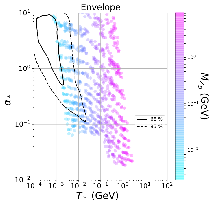
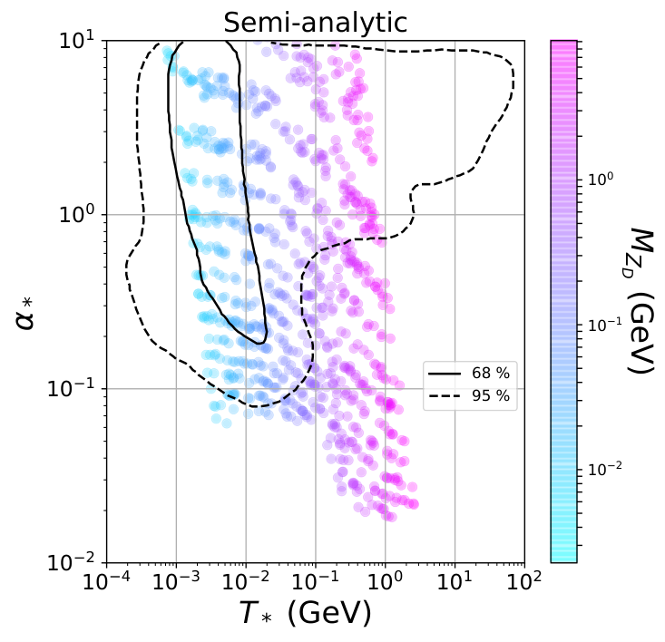
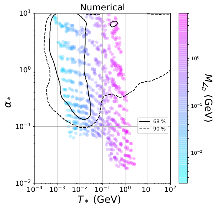
The NANOGrav collaboration, in their analysis Arzoumanian et al. 2021, has estimated the required FOPT parameters using thin shell approximation for bubble walls (envelope approximation) Jinno and Takimoto 2017b, semi-analytic approximation Lewicki and Vaskonen 2020 as well as full lattice results. Here, we present the predictions of our model (coloured points) against the backdrop of their estimates in Fig. 2. In the analysis, the gauge coupling is varied in a range corresponding to , while the gauge boson masses are shown in the colour bar. The solid ( dashed) contour corresponds to the allowed region at confidence level obtained in Arzoumanian et al. 2021 by using envelope approximation (top left panel), semi-analytic approximation (top right panel), and numerical results (bottom panel). Clearly, predictions based on light gauge boson with masses in sub-GeV regime are in better agreement with the NANOGrav findings. In order to see the strength of the FOPT in terms of parameters, we plot with respect to along with whose values are varied as shown in colour bar in Fig. 3. As can be seen from the colour bar, the strength of the phase transition increases slightly by a numerical factor when is decreased by a similar factor keeping fixed.
As mentioned above, there are three sources of GW production during a FOPT: bubble collisions, sound wave of the plasma, and turbulence of the plasma Jinno and Takimoto 2017b; Caprini et al. 2009; Hindmarsh et al. 2017; Binetruy et al. 2012; Hindmarsh et al. 2015; Caprini et al. 2016. Therefore, following Arzoumanian et al. 2021, the resultant GW power spectrum can be written as
| (33) |
In general, each contribution can be characterised by its own peak frequency and each GW spectrum can be parametrised, following Arzoumanian et al. 2021, as
| (34) |
where the pre-factor takes in account the red-shift of the GW energy density, parametrises the shape of the spectrum and is the normalization factor which depends on the bubble wall velocity . The Hubble parameter at the nucleation temperature is denoted by . Finally the peak frequency today, , is related to the value of the peak frequency at the time of emission, , as follows
| (35) |
where denotes the number of relativistic dof at the time of the FOPT. The values of the peak frequency at the time of emission, the normalisation factor, the spectral shape, and the exponents and are given in Table I of Arzoumanian et al. 2021. The efficiency factors namely, is discussed in Jinno and Takimoto 2017a; Ellis et al. 2020 and is taken from Espinosa et al. 2010; Borah et al. 2020. On the other hand, the remaining efficiency factor is taken to be approximately Arzoumanian et al. 2021. The details of bubble wall velocities and their values can be found in Steinhardt 1982; Huber and Sopena 2013; Leitao and Megevand 2015; Dorsch et al. 2018; Cline and Kainulainen 2020; Azatov and Vanvlasselaer 2021.
| 0.45 | 143 | 1.8 MeV | 0.887 | 8.23 MeV | GeV |
| 0.36 | 151 | 190 keV | 0.872 | 817 keV | GeV |
Using the above-mentioned prescription for estimating GW spectrum from a strong FOPT and by choosing a benchmark values of model
as well as FOPT parameters shown in table 1 consistent with NANOGrav data at CL, we calculate
the individual contributions to GW energy density spectrum from bubble collisions, sound wave of the plasma, and turbulence of the plasma as well as the total contribution to .
In Fig. 4,
the red, orange, cyan and black curves correspond to
the individual contribution from turbulence of the plasma, sound wave of the plasma, bubble collisions, and the total contribution to , respectively.
Due to the small value of FOPT strength parameter , as anticipated
from earlier studies Bodeker and Moore 2017; Ellis et al. 2019,
the contribution from bubble collision remains suppressed compared to the other two contributions as can be seen in Fig. 4. In Fig. 5, we show the GW spectrum for two benchmark points shown in table 1. The sensitivities of different PTA based experiments Schmitz 2020 like NANOGrav McLaughlin 2013; Arzoumanian et al. 2021; Arzoumanian et al. 2020 , SKA Weltman et al. 2020, IPTA Hobbs et al. 2010, PPTA Manchester et al. 2013, EPTA Kramer and Champion 2013 are also shown in Fig. 5. Clearly, heavier leads to shift in the peak frequency towards larger values, as expected. While the benchmark point with heavier remains barely within NANOGrav reach, the future experiments are sensitive to both the benchmark points over a much wider range of frequencies.
Dark matter: Origin of particle DM has been a longstanding puzzle. Ordinary or visible matter contributes only one-fifth to the total matter content of the present universe. The rest of the matter remain in the form of a mysterious, non-luminous, non-baryonic component, often referred to as DM. While there have been astrophysical evidences for such non-baryonic matter for several decades Zwicky 1933; Rubin and Ford 1970; Clowe et al. 2006, precision measurements of the cosmic microwave background (CMB) anisotropies at cosmology experiments like WMAP, Planck have confirmed its existence in a convincing way. The present abundance of DM is often quantified in terms of a dimensionless quantity as Aghanim et al. 2018:
| (36) |
at 68% confidence level (CL). Here is the density parameter of DM and is a dimensionless parameter of order unity. is the critical density while is the Hubble parameter. Among different particle DM proposals in the literature, the weakly interacting massive particle (WIMP) paradigm is the most appealing one. In such a scenario, a stable or sufficiently long-lived DM particle having mass and interaction strength typically around the electroweak corner can get produced thermally from the SM bath in early universe, followed by freeze-out from the bath, leaving a relic similar to the observed DM abundance Kolb and Turner 1990. Apart from this remarkable coincidence referred to as the WIMP Miracle, such DM can be probed at direct detection experiments by virtue of their sizeable interactions with SM particles like quarks Arcadi et al. 2017. However, due to absence of any such signals, alternatives to WIMP have also been discussed in recent times. One such appealing alternative is the non-thermal origin of DM, known as the feebly interacting (or freeze-in) massive particle (FIMP) DM Hall et al. 2010; Bernal et al. 2017. In such a scenario, DM has so feeble interactions with the SM particles that it never reaches thermal equilibrium, but gets produced non-thermally due to decay or scattering of SM bath particles.
As mentioned before, here we consider the vector bosons as DM candidates. This has been explored in several earlier works Diaz-Cruz and Ma 2011; Fraser et al. 2015; Bhattacharya et al. 2012; Barman et al. 2017; Barman et al. 2018; Baldes and Garcia-Cely 2019; Barman et al. 2020; Abe et al. 2020; Nomura et al. 2021; Chowdhury and Saad 2021. While most of these works considered thermal vector boson DM, the non-thermal or FIMP possibility was discussed in Barman et al. 2020. The scenario in our present model is much more simpler as SM-DM interactions occur only via the Higgs portal. As we had assumed tiny Higgs portal coupling between dark scalar and SM Higgs doublet while discussing the FOPT details, it naturally provides the freeze-in portal. Additionally, constraints from CMB measurements disfavour light sub-GeV thermal DM production in the early universe through s-channel annihilations into SM fermions Aghanim et al. 2018. Therefore, we stick to the non-thermal DM scenario here.
In general, the Boltzmann equation for comoving DM density in FIMP scenarios can be written as
| (37) |
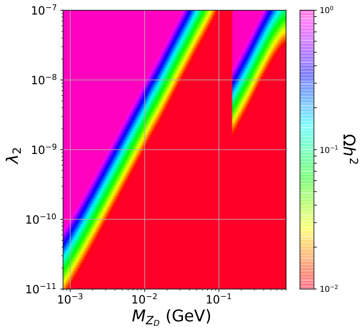
with and being the entropy density. In the above equation, we consider the freeze-in DM production from SM bath via scatterings of the type with thermal averaged cross-section denoted by . Such a scattering is mediated by scalars via mixing. In Fig. 6 (left panel), we show the evolution of comoving DM density as a function of temperature for a benchmark choice of DM mass MeV, , and . While dark gauge coupling is of order one, the smallness of leads to a tiny scalar portal mixing required for realising FIMP scenario. It should be noted that the DM abundance rises sharply around a temperature close to its mass. This is because the scalar portal mixing arises dynamically only after the symmetry breaking at a scale . On the right panel of Fig. 6, we show the parameter space in plane with DM relic as shown in the colour bar. The parameter space consistent with correct DM relic abundance shows a linear relation between and . This can be understood as follows. Since as well as quartic coupling are fixed, larger implies larger VEV of and hence larger scalar mass mediating SM-DM interactions. To compensate for this larger mediator mass, a larger mixing (and hence a larger ) is required to generate the correct DM relic. The sharp discontinuity after DM mass crosses muon mass threshold arises as it corresponds to the FOPT occurring at temperatures above the muon mass threshold, allowing muon in the radiation bath to also contribute enhancing the contribution to DM freeze-in.
Conclusion: We have studied a minimal gauge extension of the SM with the possibility of a strong first order phase transition within the dark sector, specially at a low temperature below the EW scale such that resulting stochastic GWs can be observed at PTA based experiments like NANOGrav. Motivated by the recent results from the NANOGrav 12.5 yr data providing hints of such a cosmological phase transition at sub-EW scale, we constrain our model parameters from the requirement of fitting NANOGrav data. A SFOPT occurring at sub-GeV scale can explain the NANOGrav data very well while also being sensitive to future experiments to be operating in this low frequency regime of GWs. The non-Abelian nature of our dark gauge symmetry also provides a natural vector boson DM candidate which is naturally stable due to the absence of any kinetic mixing with of the standard model at renormalisable level. Such light vector boson DM can be produced via freeze-in mechanism in the early universe. While such freeze-in mechanism is naturally realised due to tiny scalar portal couplings required to realise dark SFOPT without disturbing the EW vacuum and vice versa, it also helps in avoiding stringent CMB bounds on such light DM, if its production happens thermally. Depending upon the size of scalar portal couplings, we can have more non-trivial FOPT as well DM phenomenology which we leave for future studies.
Acknowledgements.
DB acknowledges the support from Early Career Research Award from DST-SERB, Government of India (reference number: ECR/2017/001873). AD and SKK are supported in part by the National Research Foundation (NRF) grants NRF-2019R1A2C1088953.References
- Arzoumanian et al. (2021) Z. Arzoumanian et al. (2021), eprint 2104.13930.
- Arzoumanian et al. (2020) Z. Arzoumanian et al. (NANOGrav), Astrophys. J. Lett. 905, L34 (2020), eprint 2009.04496.
- Blasi et al. (2021) S. Blasi, V. Brdar, and K. Schmitz, Phys. Rev. Lett. 126, 041305 (2021), eprint 2009.06607.
- Ellis and Lewicki (2021) J. Ellis and M. Lewicki, Phys. Rev. Lett. 126, 041304 (2021), eprint 2009.06555.
- Bian et al. (2021) L. Bian, R.-G. Cai, J. Liu, X.-Y. Yang, and R. Zhou, Phys. Rev. D 103, L081301 (2021), eprint 2009.13893.
- Ratzinger and Schwaller (2021) W. Ratzinger and P. Schwaller, SciPost Phys. 10, 047 (2021), eprint 2009.11875.
- Addazi et al. (2020) A. Addazi, Y.-F. Cai, Q. Gan, A. Marciano, and K. Zeng (2020), eprint 2009.10327.
- Nakai et al. (2021) Y. Nakai, M. Suzuki, F. Takahashi, and M. Yamada, Phys. Lett. B 816, 136238 (2021), eprint 2009.09754.
- Zhou et al. (2021) R. Zhou, L. Bian, and J. Shu (2021), eprint 2104.03519.
- Borah et al. (2021) D. Borah, A. Dasgupta, and S. K. Kang (2021), eprint 2105.01007.
- Vagnozzi (2021) S. Vagnozzi, Mon. Not. Roy. Astron. Soc. 502, L11 (2021), eprint 2009.13432.
- Caprini et al. (2016) C. Caprini et al., JCAP 1604, 001 (2016), eprint 1512.06239.
- Caprini et al. (2019) C. Caprini et al. (2019), eprint 1910.13125.
- Garcia-Bellido et al. (2021) J. Garcia-Bellido, H. Murayama, and G. White (2021), eprint 2104.04778.
- Goncharov et al. (2021) B. Goncharov et al. (2021), eprint 2107.12112.
- Jinno and Takimoto (2017a) R. Jinno and M. Takimoto, Phys. Rev. D 95, 015020 (2017a), eprint 1604.05035.
- Mohamadnejad (2020) A. Mohamadnejad, Eur. Phys. J. C 80, 197 (2020), eprint 1907.08899.
- Kim et al. (2019) Y. G. Kim, K. Y. Lee, and S.-H. Nam, Phys. Rev. D 100, 075038 (2019), eprint 1906.03390.
- Hasegawa et al. (2019) T. Hasegawa, N. Okada, and O. Seto, Phys. Rev. D 99, 095039 (2019), eprint 1904.03020.
- Marzo et al. (2019) C. Marzo, L. Marzola, and V. Vaskonen, Eur. Phys. J. C 79, 601 (2019), eprint 1811.11169.
- Hashino et al. (2018) K. Hashino, M. Kakizaki, S. Kanemura, P. Ko, and T. Matsui, JHEP 06, 088 (2018), eprint 1802.02947.
- Chiang and Senaha (2017) C.-W. Chiang and E. Senaha, Phys. Lett. B 774, 489 (2017), eprint 1707.06765.
- Schwaller (2015) P. Schwaller, Phys. Rev. Lett. 115, 181101 (2015), eprint 1504.07263.
- Baldes and Garcia-Cely (2019) I. Baldes and C. Garcia-Cely, JHEP 05, 190 (2019), eprint 1809.01198.
- Prokopec et al. (2019) T. Prokopec, J. Rezacek, and B. Świeżewska, JCAP 02, 009 (2019), eprint 1809.11129.
- Aghanim et al. (2018) N. Aghanim et al. (Planck) (2018), eprint 1807.06209.
- Schmitz (2020) K. Schmitz (2020), eprint 2002.04615.
- Weltman et al. (2020) A. Weltman et al., Publ. Astron. Soc. Austral. 37, e002 (2020), eprint 1810.02680.
- Hobbs et al. (2010) G. Hobbs, A. Archibald, Z. Arzoumanian, D. Backer, M. Bailes, N. D. R. Bhat, M. Burgay, S. Burke-Spolaor, D. Champion, I. Cognard, et al., Classical and Quantum Gravity 27, 084013 (2010), ISSN 1361-6382, URL http://dx.doi.org/10.1088/0264-9381/27/8/084013.
- Dolan and Jackiw (1974) L. Dolan and R. Jackiw, Phys. Rev. D9, 3320 (1974).
- Quiros (1999) M. Quiros, in Proceedings, Summer School in High-energy physics and cosmology: Trieste, Italy, June 29-July 17, 1998 (1999), pp. 187–259, eprint hep-ph/9901312.
- Fendley (1987) P. Fendley, Phys. Lett. B196, 175 (1987).
- Parwani (1992) R. R. Parwani, Phys. Rev. D45, 4695 (1992), [Erratum: Phys. Rev.D48,5965(1993)], eprint hep-ph/9204216.
- Arnold and Espinosa (1993) P. B. Arnold and O. Espinosa, Phys. Rev. D47, 3546 (1993), [Erratum: Phys. Rev.D50,6662(1994)], eprint hep-ph/9212235.
- Cline et al. (2008) J. M. Cline, M. Jarvinen, and F. Sannino, Phys. Rev. D 78, 075027 (2008), eprint 0808.1512.
- Mazumdar and White (2019) A. Mazumdar and G. White, Rept. Prog. Phys. 82, 076901 (2019), eprint 1811.01948.
- Hindmarsh et al. (2021) M. B. Hindmarsh, M. Lüben, J. Lumma, and M. Pauly, SciPost Phys. Lect. Notes 24, 1 (2021), eprint 2008.09136.
- Linde (1983) A. D. Linde, Nucl. Phys. B 216, 421 (1983), [Erratum: Nucl.Phys.B 223, 544 (1983)].
- Linde (1981) A. D. Linde, Phys. Lett. 100B, 37 (1981).
- Borah et al. (2020) D. Borah, A. Dasgupta, K. Fujikura, S. K. Kang, and D. Mahanta, JCAP 08, 046 (2020), eprint 2003.02276.
- Ellis et al. (2018) J. Ellis, M. Lewicki, and J. M. No (2018), [JCAP1904,003(2019)], eprint 1809.08242.
- Ellis et al. (2020) J. Ellis, M. Lewicki, and V. Vaskonen, JCAP 11, 020 (2020), eprint 2007.15586.
- Turner and Wilczek (1990) M. S. Turner and F. Wilczek, Phys. Rev. Lett. 65, 3080 (1990).
- Kosowsky et al. (1992a) A. Kosowsky, M. S. Turner, and R. Watkins, Phys. Rev. D45, 4514 (1992a).
- Kosowsky et al. (1992b) A. Kosowsky, M. S. Turner, and R. Watkins, Phys. Rev. Lett. 69, 2026 (1992b).
- Kosowsky and Turner (1993) A. Kosowsky and M. S. Turner, Phys. Rev. D47, 4372 (1993), eprint astro-ph/9211004.
- Turner et al. (1992) M. S. Turner, E. J. Weinberg, and L. M. Widrow, Phys. Rev. D46, 2384 (1992).
- Hindmarsh et al. (2014) M. Hindmarsh, S. J. Huber, K. Rummukainen, and D. J. Weir, Phys. Rev. Lett. 112, 041301 (2014), eprint 1304.2433.
- Giblin and Mertens (2014) J. T. Giblin and J. B. Mertens, Phys. Rev. D90, 023532 (2014), eprint 1405.4005.
- Hindmarsh et al. (2015) M. Hindmarsh, S. J. Huber, K. Rummukainen, and D. J. Weir, Phys. Rev. D92, 123009 (2015), eprint 1504.03291.
- Hindmarsh et al. (2017) M. Hindmarsh, S. J. Huber, K. Rummukainen, and D. J. Weir, Phys. Rev. D96, 103520 (2017), eprint 1704.05871.
- Kamionkowski et al. (1994) M. Kamionkowski, A. Kosowsky, and M. S. Turner, Phys. Rev. D49, 2837 (1994), eprint astro-ph/9310044.
- Kosowsky et al. (2002) A. Kosowsky, A. Mack, and T. Kahniashvili, Phys. Rev. D66, 024030 (2002), eprint astro-ph/0111483.
- Caprini and Durrer (2006) C. Caprini and R. Durrer, Phys. Rev. D74, 063521 (2006), eprint astro-ph/0603476.
- Gogoberidze et al. (2007) G. Gogoberidze, T. Kahniashvili, and A. Kosowsky, Phys. Rev. D76, 083002 (2007), eprint 0705.1733.
- Caprini et al. (2009) C. Caprini, R. Durrer, and G. Servant, JCAP 0912, 024 (2009), eprint 0909.0622.
- Niksa et al. (2018) P. Niksa, M. Schlederer, and G. Sigl, Class. Quant. Grav. 35, 144001 (2018), eprint 1803.02271.
- Sato (2021) R. Sato, Comput. Phys. Commun. 258, 107566 (2021), eprint 1908.10868.
- Athron et al. (2019) P. Athron, C. Balázs, M. Bardsley, A. Fowlie, D. Harries, and G. White, Comput. Phys. Commun. 244, 448 (2019), eprint 1901.03714.
- Jinno and Takimoto (2017b) R. Jinno and M. Takimoto, Phys. Rev. D 95, 024009 (2017b), eprint 1605.01403.
- Lewicki and Vaskonen (2020) M. Lewicki and V. Vaskonen (2020), eprint 2012.07826.
- Binetruy et al. (2012) P. Binetruy, A. Bohe, C. Caprini, and J.-F. Dufaux, JCAP 1206, 027 (2012), eprint 1201.0983.
- Espinosa et al. (2010) J. R. Espinosa, T. Konstandin, J. M. No, and G. Servant, JCAP 06, 028 (2010), eprint 1004.4187.
- Steinhardt (1982) P. J. Steinhardt, Phys. Rev. D25, 2074 (1982).
- Huber and Sopena (2013) S. J. Huber and M. Sopena (2013), eprint 1302.1044.
- Leitao and Megevand (2015) L. Leitao and A. Megevand, Nucl. Phys. B891, 159 (2015), eprint 1410.3875.
- Dorsch et al. (2018) G. C. Dorsch, S. J. Huber, and T. Konstandin, JCAP 1812, 034 (2018), eprint 1809.04907.
- Cline and Kainulainen (2020) J. M. Cline and K. Kainulainen (2020), eprint 2001.00568.
- Azatov and Vanvlasselaer (2021) A. Azatov and M. Vanvlasselaer, JCAP 01, 058 (2021), eprint 2010.02590.
- Bodeker and Moore (2017) D. Bodeker and G. D. Moore, JCAP 1705, 025 (2017), eprint 1703.08215.
- Ellis et al. (2019) J. Ellis, M. Lewicki, J. M. No, and V. Vaskonen, JCAP 1906, 024 (2019), eprint 1903.09642.
- McLaughlin (2013) M. A. McLaughlin, Class. Quant. Grav. 30, 224008 (2013), eprint 1310.0758.
- Manchester et al. (2013) R. N. Manchester, G. Hobbs, M. Bailes, W. A. Coles, W. van Straten, M. J. Keith, R. M. Shannon, N. D. R. Bhat, A. Brown, S. G. Burke-Spolaor, et al., Publications of the Astronomical Society of Australia 30 (2013), ISSN 1448-6083, URL http://dx.doi.org/10.1017/pasa.2012.017.
- Kramer and Champion (2013) M. Kramer and D. J. Champion, Classical and Quantum Gravity 30, 224009 (2013), URL https://doi.org/10.1088/0264-9381/30/22/224009.
- Zwicky (1933) F. Zwicky, Helv. Phys. Acta 6, 110 (1933), [Gen. Rel. Grav.41,207(2009)].
- Rubin and Ford (1970) V. C. Rubin and W. K. Ford, Jr., Astrophys. J. 159, 379 (1970).
- Clowe et al. (2006) D. Clowe, M. Bradac, A. H. Gonzalez, M. Markevitch, S. W. Randall, C. Jones, and D. Zaritsky, Astrophys. J. 648, L109 (2006), eprint astro-ph/0608407.
- Kolb and Turner (1990) E. W. Kolb and M. S. Turner, Front. Phys. 69, 1 (1990).
- Arcadi et al. (2017) G. Arcadi, M. Dutra, P. Ghosh, M. Lindner, Y. Mambrini, M. Pierre, S. Profumo, and F. S. Queiroz (2017), eprint 1703.07364.
- Hall et al. (2010) L. J. Hall, K. Jedamzik, J. March-Russell, and S. M. West, JHEP 03, 080 (2010), eprint 0911.1120.
- Bernal et al. (2017) N. Bernal, M. Heikinheimo, T. Tenkanen, K. Tuominen, and V. Vaskonen, Int. J. Mod. Phys. A32, 1730023 (2017), eprint 1706.07442.
- Diaz-Cruz and Ma (2011) J. L. Diaz-Cruz and E. Ma, Phys. Lett. B 695, 264 (2011), eprint 1007.2631.
- Fraser et al. (2015) S. Fraser, E. Ma, and M. Zakeri, Int. J. Mod. Phys. A 30, 1550018 (2015), eprint 1409.1162.
- Bhattacharya et al. (2012) S. Bhattacharya, J. L. Diaz-Cruz, E. Ma, and D. Wegman, Phys. Rev. D 85, 055008 (2012), eprint 1107.2093.
- Barman et al. (2017) B. Barman, S. Bhattacharya, S. K. Patra, and J. Chakrabortty, JCAP 12, 021 (2017), eprint 1704.04945.
- Barman et al. (2018) B. Barman, S. Bhattacharya, and M. Zakeri, JCAP 09, 023 (2018), eprint 1806.01129.
- Barman et al. (2020) B. Barman, S. Bhattacharya, and M. Zakeri, JCAP 02, 029 (2020), eprint 1905.07236.
- Abe et al. (2020) T. Abe, M. Fujiwara, J. Hisano, and K. Matsushita, JHEP 07, 136 (2020), eprint 2004.00884.
- Nomura et al. (2021) T. Nomura, H. Okada, and S. Yun, JHEP 06, 122 (2021), eprint 2012.11377.
- Chowdhury and Saad (2021) T. A. Chowdhury and S. Saad (2021), eprint 2107.11863.