Surface chemistry models for GaAs epitaxial growth and hydride cracking using reacting flow simulationsPreprint: AIP/123-QED

The configuration simulated in this work (see illustration in Fig. 1) is from experimental studies by Schulte et al. 2018 that used a Dynamic-Hydride Vapor phase epitaxy (D-HVPE) reactor where growth rates with uncracked arsine were also reported. These experiments were conducted with a Dynamic-Hydride Vapor phase epitaxy (D-HVPE) reactor Young et al. 2013 which addresses manufacturing challenges posed by HVPE. Highly efficient thin-film solar cells typically consist of several layers, each one made of a different III-V compound Biefeld, Koleske, and Cederberg 2015. When the growth rate of the solar cell is low enough and the reactor equilibrates quickly, the substrate can be kept idle in the same chamber while different external gas are injected over time. With a higher growth rate and large residence time of gases - such as in HVPE deposition reactors - this strategy can lead to non-abrupt interfaces between the layers, which is detrimental to solar cell efficiency. In the D-HVPE, the aforementioned issue is avoided by physically moving the substrate to a different chamber each time a new layer needs to be grown. In order to prevent inter-chamber flow contamination, the chambers are separated by vertical gas curtains created by a flow of H2 (see illustration in Fig. 1).

The D-HVPE reactor considered here has been experimentally Metaferia et al. 2019; Schulte et al. 2018; Schulte et al. 2019 and numerically McClure et al. 2020; Schulte et al. 2019 shown to provide high growth rate and efficiency, while potentially enabling in-line manufacturing.

The metal-halide is generated in-situ by injecting HCl into a boat/reservoir of liquid Ga. The boat is externally heated at $1073.15$ K to drive the kinetics of the HCl + Ga${}\mathrel{\mathop{\makebox[0.0pt]{\rightarrow\displaystyle}}\limits}{}$GaCl reaction. The boat conversion efficiency was previously estimated to be 90% Schulte et al. 2016. It outputs a mixture of gaseous gallium chloride GaCl and residual HCl that were not converted. A center port (called inlet A in Schulte et al. 2018) introduces a mixture of $\text{AsH}{\vphantom{\text{X}}}_{\smash[t]{\text{3}}}$ and $\text{H}{\vphantom{\text{X}}}_{\smash[t]{\text{2}}}$ in the chamber. The reactants are then deposited on a substrate externally heated at $923.15$ K. In Fig. 1, the external heating is represented by the red and blue dashed boxes.

The dataset used for validation of our model is that presented in Schulte et al. 2018 where growth rates at the center of the substrate were measured under a variety of flow conditions. The volume flow rates at standard pressure and temperature for all the cases considered are shown in Tab. 1. The experiments were conducted at a pressure of $0.829$ atm and with external gas injected at ambient temperature.

An important observation from the experiment was the near-zero growth of GaAs when $\text{AsH}{\vphantom{\text{X}}}_{\smash[t]{\text{3}}}$ was recirculated into the reactor (through inlet B in Fig. 1) similar to GaCl rather than direct injection through the center port (inlet A in Fig. 1). The larger residence time of $\text{AsH}{\vphantom{\text{X}}}_{\smash[t]{\text{3}}}$ in this case led to increased cracking at the reactor walls before reaching the substrate. This hypothesis is further bolstered by the success of growth rate models that considered a deposition pathway only via cracked arsine Schulte et al. 2019. Under the conditions where all the arsine has cracked and in the range of operating conditions investigated, an equilibrium kinetic model Schulte et al. 2016 indeed predicts growth rates of at most $2$ $\mu$m/h (Fig. 2) which is at least one order of magnitude lower than growth rates measured in Schulte et al. 2018. Here, the $\text{As}{\vphantom{\text{X}}}_{\smash[t]{\text{4}}}$ pathway is inhibited by the low residence time of external gas sources and the low substrate temperature. Therefore, the growth rate available in Schulte et al. 2018 is particularly suited to deduce a kinetic model for the $\text{AsH}{\vphantom{\text{X}}}_{\smash[t]{\text{3}}}$-pathway for epitaxial growth.

The surface reaction is modeled as an irreversible forward reaction

The assumption of irreversibility is justified by its large equilibrium constant which suggests that the backward reaction is unlikely McClure et al. 2020; Grüter et al. 1989. A finite rate chemistry model is developed hereafter for the forward reaction. An infinitely fast model is also constructed and the results are reported in App. F.

The finite rate chemistry model for the reaction at the substrate is constructed by assuming the Arrhenius form $K_{reac}=A_{reac}T^{\beta_{reac}}exp(-Ea_{reac}/R_{u}T)$, where $A_{reac}$, $\beta_{reac}$ are kinetic constants and $Ea_{reac}$ is the activation energy. In the experiments conducted in Schulte et al. 2018, it was found that for the temperature range $[873-953~K]$, the dependence of the epitaxial growth rate with temperature was negligible. Therefore, $K_{reac}$ is assumed to be independent of temperature over similar temperature ranges studied in this work.

The objective of this section is to find a value of $K_{reac}$. The CFD model is used to simulate the D-HVPE reactor with different values of $K_{reac}$. The resulting growth rates are obtained by computing the molar flux of $\text{AsH}{\vphantom{\text{X}}}_{\smash[t]{\text{3}}}$ at the substrate, which is equal to the number of moles of GaAs produced. The density of GaAs(s) is then used to compute the growth rate obtained via CFD, which is then compared to the ones reported in the Schulte et al. 2018. The growth rates are measured at the center of the substrate.

Eleven values of $K_{reac}$ are chosen within the range [$45$ m.s^-1,$310$ m.s^-1]. For each value of $K_{reac}$, the seven cases shown in Tab. 1 are simulated. In absence of uncertainty, a total of $77$ numerical simulations would be needed for calibration. In the present case, the optimal value of $K_{reac}$ depends on the value of $A_{cracking}$ obtained by fitting the cracking model. To account for uncertainty in the value of $A_{cracking}$, the calibration procedure is conducted for ten values of $A_{cracking}$ chosen in the range [$6.5\times 10^{5}$ m.s^-1,$8.5\times 10^{5}$ m.s^-1], which span the support of its posterior distribution. The function that related $K_{reac}$ and $A_{cracking}$ is then convolved with the posterior distribution of $A_{cracking}$ to deduce the PDF of $K_{reac}$. The overall procedure is illustrated in Fig. 5 and requires a total of $770$ runs.

Due to the large number of simulations required, the calibration is done with the coarse grid ($0.5$ million computational cells). The fine mesh ($1$ million computational cells) is used afterwards to verify grid convergence for the estimated values of $K_{reac}$.

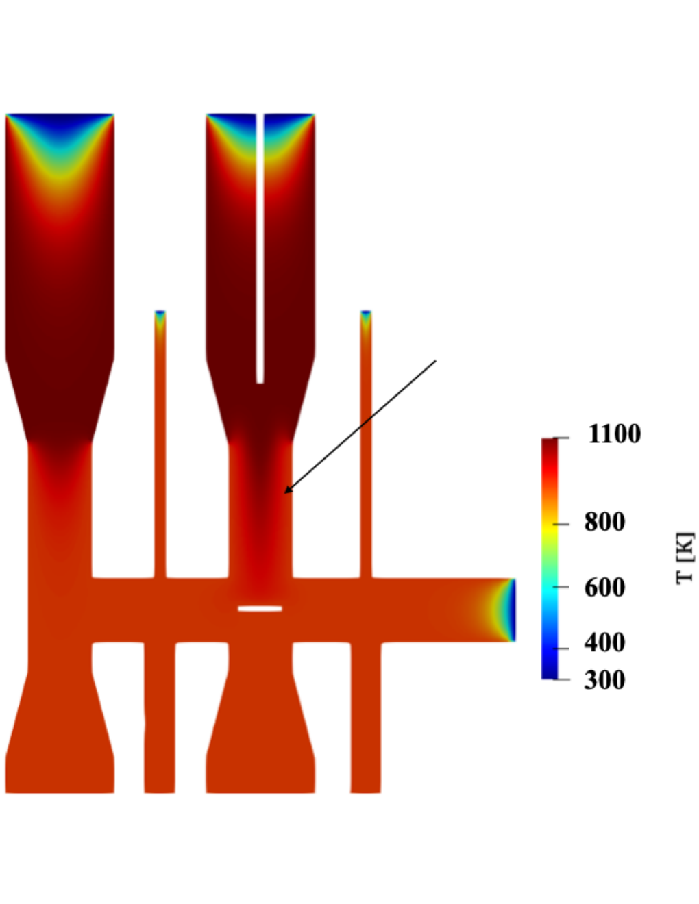
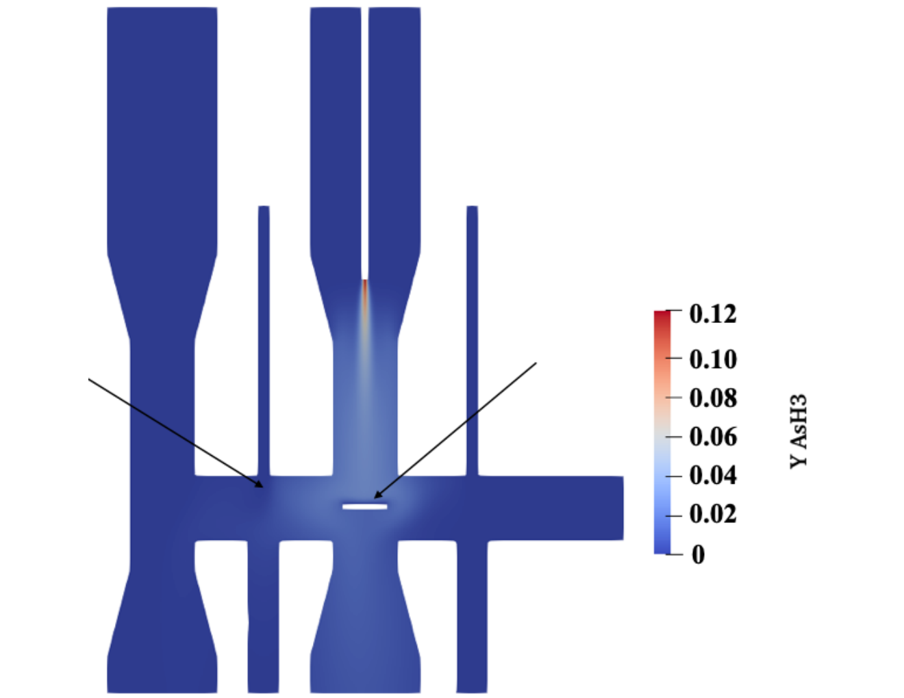
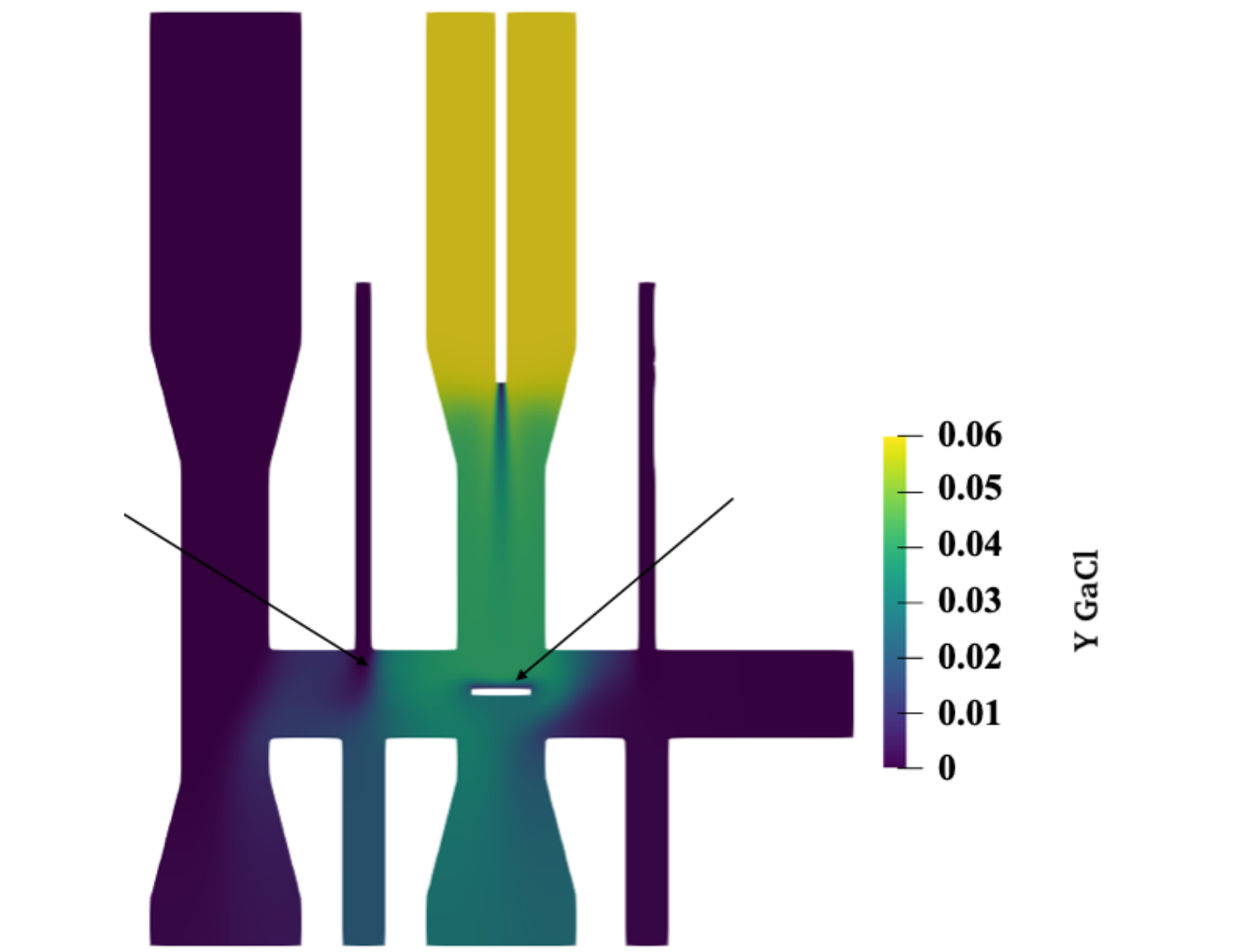
The steady-state distribution of temperature and arsine mass fraction for case 3 (Tab. 1) with $K_{reac}=222.8$ m.s^-1 and $A_{cracking}=8.5\times 10^{5}$ m.s^-1 is illustrated in Fig. 6. It can be seen that since the flow inside the center port is heated to a temperature close to $1073.15$ K, the center port injects a hot flow at the substrate (indicated by the arrow). The contour of $\text{AsH}{\vphantom{\text{X}}}_{\smash[t]{\text{3}}}$ (bottom) shows the effect of the flow curtain which avoids contamination of the adjacent chamber with arsine (left arrow). At the substrate, $\text{AsH}{\vphantom{\text{X}}}_{\smash[t]{\text{3}}}$ is consumed, which results in a non-zero normal gradient (right arrow). Similar features can be observed for GaCl.

For each $(K_{reac},A_{cracking})$ sample pair, the average error in growth rate $\langle\varepsilon\rangle$ over the seven cases considered is computed. The results are shown in Fig. 7. It can be seen that there exists an optimal value of $K_{reac}$ which leads to the best match of the growth rates. In the particular case considered ($A_{cracking}=8.5\times 10^{5}$ m.s^-1), $K_{reac}=222.8$ m.s^-1 minimizes $\langle\varepsilon\rangle$. To improve the estimate of the value of $K_{reac}$ that minimizes the error, interpolation between data points is done with radial basis functions, where hyperparameters are optimized using the Scikit-Learn library Pedregosa et al. 2011. An example of the interpolation result is shown in Fig. 7.

Over the range chosen $K_{reac}$, it can be observed from Fig. 7 that there exists a value that can serve, at least, as a global minimizer of the discrepancy with experimental results. It is shown here, that the local minimum is likely a global minimum. We first argue that the relationship between the rate of growth $R_{G}$ and the kinetic coefficient $K_{reac}$ is monotonic and increasing. Physically, this assertion is justified by the fact that increasing the kinetic rate should increase the rate of production of GaAs. We also propose a numerical argument by plotting the difference between the rate of growth obtained in the simulations ($R_{G,sim}$) and in experiments ($R_{G,exp}$) for all $A_{cracking}$ and all $K_{reac}$ values. The results are shown in Fig. 8 (top). As expected, the rate of growth is monotonically increasing with $K_{reac}$ for all $A_{cracking}$ values. Next, we record the minimum and maximum error over all the cases for each $A_{cracking}$ and $K_{reac}$. Because of the monotonically increasing relation between $K_{reac}$ and $R_{G}$, if the maximum error $R_{G,sim}-R_{G,exp}$ at the lowest $K_{reac}$ value is negative, then $\forall K_{reac}<45$ m.s^-1, $\langle\varepsilon\rangle$ would be larger than for $K_{reac}=45$ m.s^-1 . In Fig. 8 (right), it can be seen that the maximum absolute value of the error is almost negative for all $A_{cracking}$ at $K_{reac}=45$ m.s^-1. The same argument can be invoked for the minimum error at $K_{reac}=310$ m.s^-1 which is positive. We therefore argue that the minimum shown is likely a global minimum.

The growth rates computed with $K_{reac}=222.8$ m.s^-1 and $A_{cracking}=8.5\times 10^{5}$ m.s^-1 are plotted against experimental values in Fig. 9. A reasonable agreement with experiments can be observed. Furthermore, the trends are consistent with the experiments and physical intuition. As the volume flow rate of $\text{H}{\vphantom{\text{X}}}_{\smash[t]{\text{2}}}$, $Q_{a}$ through the center port increases (left), less $\text{AsH}{\vphantom{\text{X}}}_{\smash[t]{\text{3}}}$ cracks which leads to larger reaction rates. The exponential dependence of the amount of cracked $\text{AsH}{\vphantom{\text{X}}}_{\smash[t]{\text{3}}}$ with the velocity (Eq. 17) should result in a super-linear increase of growth rate with the flow rate of arsine through the center port. This is the trend observed in the experiments and the simulations. This observation is in sharp contrast with the linear increase of the growth rate with increasing concentration of GaCl (bottom). To ensure that the calibrated $K_{reac}$ is only minimally affected by the numerical errors, the fine grid (1 million computational cells) is used to verify that the results are grid converged. The fine and coarse grids predict similar growth rates and therefore the baseline grid is sufficient for accurate predictions.

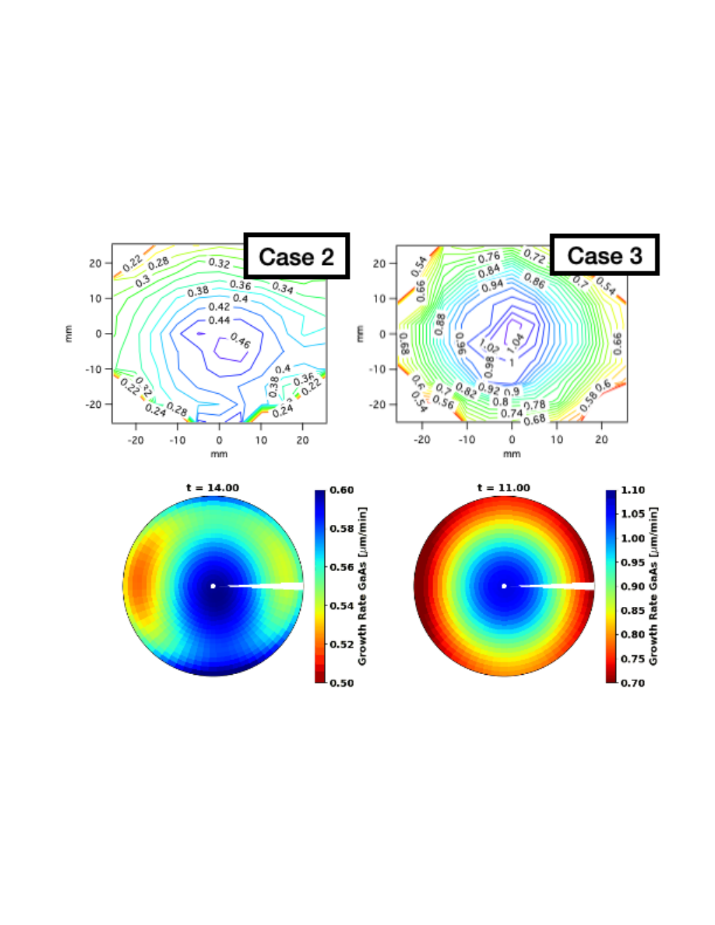
The spatial distribution of the growth rate at the substrate is compared to experimental data in Fig. 10. A reasonable agreement can be observed for case 3 (strong flow through the center port). A breakdown of the axial symmetry can be observed for case 2 (weaker flow through the center port) both in simulation and experimental data. The apparent breakdown of symmetry typically appears at low center port velocity, such as the one of Case 2. The flow near the substrate is influenced by a vertical component that originates from the center port, and by a horizontal component, the crossflow that connects the two deposition chambers. The horizontal flow can be observed in Fig. 6 (middle and bottom). When lower center port velocities are used, the relative effect of the horizontal crossflow may increase and disturb the boundary layer near the substrate, thereby leading to a breakdown of growth symmetry. Interestingly, the same symmetry breakdown seems to occur in the experimental results, albeit to a smaller extent. The discrepancy may be due to a slightly earlier center port jet breakdown in the simulations due to either numerical diffusion, or errors in the center jet exit boundary conditions. Finally, we note that in other experiments reported for the same reactor Schulte et al. 2019, a similar breakdown of symmetry may appear at different conditions. This result suggests that the model can be used not only to assess the overall growth rate of the substrate but also its spatial uniformity, which is critical for the efficiency of solar cells.

As explained in Sec. V.2, the calibration procedure is repeated for ten different values of $A_{cracking}$ which span the support of its posterior distribution obtained in Sec. IV. As a result, one obtains the response curve of the optimal $K_{reac}$ as a function of $A_{cracking}$, which is shown in Fig. 11 (top). As $A_{cracking}$ increases, the amount of $\text{AsH}{\vphantom{\text{X}}}_{\smash[t]{\text{3}}}$ that reaches the substrate decreases. Therefore, to keep constant the growth rates, the optimal $K_{reac}$ is a monotonically increasing function of $A_{cracking}$. This trend can be observed in Fig. 11. It can however be seen that the increase occurs by steps which is a consequence of the discretization of $A_{cracking}$. Given the dependence of $K_{reac}$ with $A_{cracking}$, one can sample $A_{cracking}$ using a Markov-chain Monte Carlo (MCMC) approach and construct a PDF of $K_{reac}$. The results are shown in Fig. 11 (bottom). The standard deviation of the PDF of $K_{reac}$ can then be used to extract uncertainty bounds on the calibrated value of the kinetic parameter. We found $K_{reac}=205\pm 5$ m.s^-1

References

- King et al. (2006) R. R. King, C. M. Fetzer, D. C. Law, K. M. Edmondson, H. Yoon, G. S. Kinsey, D. D. Krut, J. H. Ermer, P. Hebert, B. T. Cavicchi, et al., “Advanced III-V multijunction cells for space,” in 2006 IEEE 4th World Conference on Photovoltaic Energy Conference, Vol. 2 (IEEE, 2006) pp. 1757–1762.
- Hoheisel, Philipps, and Bett (2010) R. Hoheisel, S. Philipps, and A. Bett, “Long-term energy production of III–V triple-junction solar cells on the Martian surface,” Progress in Photovoltaics: Research and Applications 18, 90–99 (2010).
- Simon et al. (2019) J. Simon, K. L. Schulte, K. A. Horowitz, T. Remo, D. L. Young, and A. J. Ptak, “III-V-based optoelectronics with low-cost dynamic hydride vapor phase epitaxy,” Crystals 9, 3 (2019).
- McClure et al. (2020) E. L. McClure, K. L. Schulte, J. Simon, W. Metaferia, and A. J. Ptak, “Gaas growth rates of 528 m/h using dynamic-hydride vapor phase epitaxy with a nitrogen carrier gas,” Applied Physics Letters 116, 182102 (2020).
- Metaferia et al. (2019) W. Metaferia, K. L. Schulte, J. Simon, S. Johnston, and A. J. Ptak, “Gallium arsenide solar cells grown at rates exceeding 300 m/h by hydride vapor phase epitaxy,” Nature communications 10, 1–8 (2019).
- Horowitz et al. (2018) K. A. Horowitz, T. W. Remo, B. Smith, and A. J. Ptak, “A techno-economic analysis and cost reduction roadmap for III-V solar cells,” Tech. Rep. (National Renewable Energy Lab.(NREL), Golden, CO (United States), 2018).
- Schulte et al. (2018) K. L. Schulte, A. Braun, J. Simon, and A. J. Ptak, “High growth rate hydride vapor phase epitaxy at low temperature through use of uncracked hydrides,” Applied Physics Letters 112, 042101 (2018).
- Hollan and Durand (1979) L. Hollan and J. Durand, “Fast growth in GaAs VPE at low temperature and high partial pressures,” Journal of Crystal Growth 46, 665–670 (1979).
- DenBaars et al. (1986) S. DenBaars, B. Maa, P. Dapkus, A. Danner, and H. C. Lee, “Homogeneous and heterogeneous thermal decomposition rates of trimethylgallium and arsine and their relevance to the growth of gaas by mocvd,” Journal of Crystal Growth 77, 188–193 (1986).
- Shaw (1975) D. W. Shaw, “Kinetic aspects in the vapour phase epitaxy of III–V compounds,” Journal of crystal growth 31, 130–141 (1975).
- Kangawa et al. (2002) Y. Kangawa, T. Ito, Y. Hiraoka, A. Taguchi, K. Shiraishi, and T. Ohachi, “Theoretical approach to influence of As2 pressure on GaAs growth kinetics,” Surface science 507, 285–289 (2002).
- Young et al. (2013) D. L. Young, A. J. Ptak, T. F. Kuech, K. Schulte, and J. D. Simon, “High throughput semiconductor deposition system,” (2013), uS Patent App. 13/895,190.
- Biefeld, Koleske, and Cederberg (2015) R. M. Biefeld, D. D. Koleske, and J. G. Cederberg, “The Science and Practice of Metal-Organic Vapor Phase Epitaxy (MOVPE),” in Handbook of Crystal Growth (Elsevier, 2015) pp. 95–160.
- Schulte et al. (2019) K. L. Schulte, W. Metaferia, J. Simon, and A. J. Ptak, “Uniformity of GaAs solar cells grown in a kinetically-limited regime by dynamic hydride vapor phase epitaxy,” Solar Energy Materials and Solar Cells 197, 84–92 (2019).
- Schulte et al. (2016) K. L. Schulte, J. Simon, N. Jain, D. L. Young, and A. J. Ptak, “A kinetic model for GaAs growth by hydride vapor phase epitaxy,” in 2016 IEEE 43rd Photovoltaic Specialists Conference (PVSC) (IEEE, 2016) pp. 1930–1933.
- Harrous et al. (1988) M. Harrous, L. Chaput, A. Bendraoui, M. Cadoret, C. Pariset, and R. Cadoret, “Phosphine and arsine decomposition in CVD reactors for InP and InGaAs growth,” Journal of Crystal Growth 92, 423–431 (1988).
- Braman, Oliver, and Raman (2013) K. Braman, T. A. Oliver, and V. Raman, “Bayesian analysis of syngas chemistry models,” Combustion Theory and Modelling 17, 858–887 (2013).
- Bell et al. (2019) J. Bell, M. Day, J. Goodman, R. Grout, and M. Morzfeld, “A bayesian approach to calibrating hydrogen flame kinetics using many experiments and parameters,” Combustion and Flame 205, 305–315 (2019).
- Grüter et al. (1989) K. Grüter, M. Deschler, H. Jürgensen, R. Beccard, and P. Balk, “Deposition of high quality GaAs films at fast rates in the LP-CVD system,” Journal of crystal growth 94, 607–612 (1989).
- Pedregosa et al. (2011) F. Pedregosa, G. Varoquaux, A. Gramfort, V. Michel, B. Thirion, O. Grisel, M. Blondel, P. Prettenhofer, R. Weiss, V. Dubourg, J. Vanderplas, A. Passos, D. Cournapeau, M. Brucher, M. Perrot, and E. Duchesnay, “Scikit-learn: Machine Learning in Python,” Journal of Machine Learning Research 12, 2825–2830 (2011).
- Hassanaly et al. (2018) M. Hassanaly, H. Koo, C. F. Lietz, S. T. Chong, and V. Raman, “A minimally-dissipative low-Mach number solver for complex reacting flows in OpenFOAM,” Computers & Fluids 162, 11–25 (2018).
- Hassanaly et al. (2020) M. Hassanaly, Y. Tang, S. Barwey, and V. Raman, “Data-driven Analysis of Relight variability of Jet Fuels induced by Turbulence,” Combustion and Flame 225, 453–467 (2020).
- Tang and Raman (2021) Y. Tang and V. Raman, “Large eddy simulation of premixed turbulent combustion using a non-adiabatic, strain-sensitive flamelet approach,” Combustion and Flame 234, 111655 (2021).
- Koo et al. (2017) H. Koo, M. Hassanaly, V. Raman, M. E. Mueller, and K. Peter Geigle, “Large-eddy simulation of soot formation in a model gas turbine combustor,” Journal of Engineering for Gas Turbines and Power 139 (2017).
- Sitaraman et al. (2021) H. Sitaraman, S. Yellapantula, M. T. H. de Frahan, B. Perry, J. Rood, R. Grout, and M. Day, “Adaptive mesh based combustion simulations of direct fuel injection effects in a supersonic cavity flame-holder,” Combustion and Flame 232, 111531 (2021).
- Smagorinsky (1963) J. Smagorinsky, “General circulation experiments with the primitive equations: I. The basic experiment,” Monthly weather review 91, 99–164 (1963).
- Tang et al. (2019) Y. Tang, M. Hassanaly, V. Raman, B. Sforzo, and J. Seitzman, “A comprehensive modeling procedure for estimating statistical properties of forced ignition,” Combustion and Flame 206, 158–176 (2019).
- Maestri and Cuoci (2013) M. Maestri and A. Cuoci, “Coupling CFD with detailed microkinetic modeling in heterogeneous catalysis,” Chemical Engineering Science 96, 106–117 (2013).
- Strang (1968) G. Strang, “On the construction and comparison of difference schemes,” SIAM journal on numerical analysis 5, 506–517 (1968).
- Heye, Raman, and Masri (2013) C. Heye, V. Raman, and A. R. Masri, “LES/probability density function approach for the simulation of an ethanol spray flame,” Proceedings of the Combustion Institute 34, 1633–1641 (2013).
- Chong et al. (2018) S. T. Chong, M. Hassanaly, H. Koo, M. E. Mueller, V. Raman, and K.-P. Geigle, “Large eddy simulation of pressure and dilution-jet effects on soot formation in a model aircraft swirl combustor,” Combustion and Flame 192, 452–472 (2018).
- Oehlschlaeger et al. (2009) M. A. Oehlschlaeger, J. Steinberg, C. K. Westbrook, and W. J. Pitz, “The autoignition of iso-cetane at high to moderate temperatures and elevated pressures: Shock tube experiments and kinetic modeling,” Combustion and flame 156, 2165–2172 (2009).
- Kee et al. (1999) R. Kee, G. Dixon-Lewis, J. Warnatz, M. Coltrin, J. Miller, and H. Moffat, “Transport: a software package for the evaluation of gas-phase, multicomponent transport properties,” Chemkin Collection (1999).
- Bergman et al. (2011) T. L. Bergman, F. P. Incropera, D. P. DeWitt, and A. S. Lavine, Fundamentals of heat and mass transfer (John Wiley & Sons, 2011).