Dynamic Mixture of Experts Models for Online Prediction
Abstract
A mixture of experts models the conditional density of a response variable using a mixture of regression models with covariate-dependent mixture weights. We extend the finite mixture of experts model by allowing the parameters in both the mixture components and the weights to evolve in time by following random walk processes. Inference for time-varying parameters in richly parameterized mixture of experts models is challenging. We propose a sequential Monte Carlo algorithm for online inference and based on a tailored proposal distribution built on ideas from linear Bayes methods and the EM algorithm. The method gives a unified treatment for mixtures with time-varying parameters, including the special case of static parameters. We assess the properties of the method on simulated data and on industrial data where the aim is to predict software faults in a continuously upgraded large-scale software project.
Keywords: Bayesian sequential inference, Linear Bayes, Particle filtering, Mixture models, Sequential Monte Carlo.
1 Introduction
A mixture of experts (ME) model (Jordan and Jacobs 1994) provides a flexible framework for expressing the distribution of a response variable conditional on a set of covariates. It models continuous or discrete response variables using a finite mixture model with covariate-dependent component models and mixture weights. The component models are commonly referred to as the experts and the mixture weights models as gates. Generally, the experts are regression models with the response’s conditional density from the exponential family; see Gormley and Frühwirth-Schnatter 2018 for a concise introduction to ME models and Yuksel et al. 2012 for an extensive list of application areas.
ME models have been extended in many ways. Hunter and Young 2012 relax the parametric assumption of the component models and propose a semi-parametric inference methodology for mixtures of linear regression models. Villani et al. 2012 extend the component models to density functions outside the exponential family and use Bayesian variable selection in all parts of the model. Jacobs et al. 1997 propose a Bayesian hierarchical model in which the conditional density of the response is expressed as a mixture of ME components. Rasmussen and Ghahramani 2002 propose an infinite mixture of Gaussian process experts. Zeevi et al. 1996 and Carvalho and Tanner 2005a; Carvalho and Tanner 2005b extend the ME model framework to autoregressive time series data where the covariates may include lagged values of the response and they study the properties of the maximum likelihood estimator. Wood et al. 2002 propose a Bayesian inference methodology for ME models and allow smoothing spline components. In longitudinal data applications, Muthén and Shedden 1999 consider fixed and random effect covariates in both components and mixture weights. Quiroz and Villani 2013 propose a ME model with static parameters for longitudinal data but where the subjects are allowed to dynamically change mixture components over time.
While many existing ME models discussed in the previous paragraph are very flexible, they are still too restrictive for many applications, in particular when: i) the data is an irregularly spaced time series or arrives in batches; ii) the conditional density of the response tends to change over time. Our application to predicting software faults, in Section 4, is one such typical example taken from industry. Software is generally upgraded at irregular times - a week may pass without any release followed by two or three releases in the next week - depending on the bugs reported in previous versions, the complexity of the added features in the release, or business related factors. Also, the distribution of the response variable naturally changes as the software matures: the developers in the project change over time, user behavior changes, and new technologies emerge which demand adaptation. All these issues make standard ME models for time series data impractical.
We extend the class of ME models to dynamic mixture of experts (DME) models to propose an online (real-time) predictive model with time-varying parameters. The new class is particularly suited for unstructured streaming data, but may also be used for equally spaced time series with time-varying distributions. The proposed DME models have the general form of varying-regression coefficient models (Hastie and Tibshirani 1993); the regression coefficients in both the mixture components and the mixture weights are allowed to vary over time through a latent process. The latent process can be modelled as a discrete first order Markov process with static (Liehr et al. 1999; Kohlmorgen et al. 2000) or time-varying (Wang et al. 2003) transition probabilities. Alternatively, it can be modelled through random walk processes (West et al. 1985; Fahrmeir et al. 2004; Fahrmeir and Kneib 2011) as in Section 2.1. The density for the response variable is modelled conditional on the value of the latent state. This allows the model to adapt locally to any abrupt changes through time (Fahrmeir et al. 2004). Also, it facilitates designing an adaptive online (real-time) Bayesian predictive inference in which the uncertainty is updated sequentially as new data arrive and predictions are computed based on the recently updated posterior density - the posterior; see Section 3.
Inference in mixture models is challenging. One challenge is the identifiability issue caused by the invariance of the likelihood under permutation of component labels and parameters. Constraints on the regression coefficients have been imposed to identify ME models, see (Jiang and Tanner 1999) and Appendix B. However, identifiability is of less importance in applications where prediction is the main objective as the predictive distribution is unaffected by label switching (Geweke 2007). Another important issue in mixture models is the number of components. One strand of the literature use nonparametric Bayes approaches with infinite mixtures typically modeled by stick-breaking processes (Hjort et al. 2010), or reversible jump MCMC (Richardson and Green 1997) to obtain the posterior over the number of mixture components. Another line of research uses model comparison methods to select the optimal number of components (Celeux et al. 2019; Geweke and Keane 2007). In addition to these issues, the structure of DME models brings additional challenges. DME are often richly parameterized with time-varying regression coefficients in both the components and the mixture weights. This leads to a high dimensional and complex target posterior that can only be properly explored by carefully designed numerical methods.
We propose online inference based on Sequential Monte Carlo (SMC) methods (Del Moral et al. 2006; Doucet et al. 2000) to address these issues. The performance of SMC methods depends on the proposal/importance distribution from which parameters are sampled. Given the complexity of DME models, off-the-shelf SMC methods based on commonly used proposal distributions such as the bootstrap filter will perform poorly. Our main contribution is a proposal distribution tailored to the class of DME models. The potentially high-dimensional regression coefficients influence the conditional density only through the low-dimensional linear predictors transformed by the link functions. This makes it possible to combine the linear Bayes method (West et al. 1985) and ideas from the expectation and maximization (EM) algorithm principle (Dempster et al. 1977) to build the proposal distribution efficiently. Our algorithm builds on the marginal particle filter algorithm (Klaas et al. 2005) for online (real-time) prediction; offline inference using SMC algorithms can be done following ideas in Munezero 2021, where the proposed methodology can be considered as an integrated part of the particle smoother.
Standard inference for mixture models requires posterior draws of component allocation indicators or, in the approach of Carvalho et al. 2010, to keep track of the number of allocations for each component and conditional sufficient statistics for the mixture component parameters. Our methodology expresses the likelihood in its marginal form, which does not require sampling component indicators, hence reducing considerably the dimension of the target posterior. The posterior’s dimension is reduced even further by using the discount factor approach (West et al. 1985) that recursively estimates the innovation variance of the states at a particular time point as a function of a discount factor and the filtered information from the most recent posterior. This means that the inference requires keeping track of only the regression coefficients through time.
The smoothness of the regression coefficients evolution is controlled via which allows building static and dynamic models in a unified way just by changing the value of . Liu and West 2001 suggest that models with are essentially static, and those with are dynamic, although this rule of thumb may vary depending on applications. Inference on the discount factor and the number of components is performed using the log predictive score, a marginal likelihood-based model comparison criteria (Geweke and Keane 2007; Villani et al. 2009).
The proposed methodology allows writing general computer code where a user can easily add a new model by supplying the first and second derivative of the component densities with respect to the linear predictors, which are the only key arguments of our procedure. Recent advances in automatic differentiation (Baydin et al. 2018) even removes the requirement of computing derivatives analytically.
The rest of the paper is organized as follows. Section 2 introduces the dynamic mixture of experts model and the prior process. Section 3 presents the SMC algorithm based on a proposal distribution from linear Bayes theory. Section 4 presents an industrial application to online prediction of faults in a large-scale software project, where allowing parameters to evolve over time considerably improves predictive performance. Section 5 explores the properties of the inference method on simulated data. The final section concludes.
2 Dynamic mixture of experts
Let represent data from a time dependent process observed at different time points , where denotes the univariate response variable and is a -dimensional covariate vector. The may contain only one observation as in standard time series applications, or it may be a data batch containing several observations as in the software upgrade process described in Section 4. We propose the dynamic mixture of experts model
| (2.1) |
for online (real time) prediction of given the value of the covariate ; and are subsets of of dimensions and respectively. The and , , are time-varying covariate-dependent parameter and mixture weight functions of the expert model respectively, and . The covariates in the mixture weights can be distinct from the covariates in the experts.
Here, the experts represent the component models in the mixture (2.1) and they depend on the structure of the response variable; they are typically density functions from the exponential family, e.g. Gaussian if is continuous, or Poisson, binomial or negative binomial for count data, or multinomial if is categorical. However, as in Villani et al. 2012, we allow the component models to be any well-behaved density functions, not necessarily limited to the exponential family, and the model parameter may be multidimensional with each of its components connected to the covariates through its own link function. By well-behaved densities we mean densities that are twice differentiable with respect to the parameters, and that satisfies the nondegeneracy condition in Jiang and Tanner 1999 so that the mixture of experts model is identified. Jiang and Tanner 1999 show that this condition is fulfilled for Poisson components and Section B in the Appendix give a similar result for generalized Poisson components, which do not belong to the exponential family and are used in the empirical application in Section 4.
The component model parameters , are connected to their linear predictors through a link function as
| (2.2) |
where and . For component models with more than one parameter, Eq. 2.1 can be extended by linking each parameter to its own linear predictor; see Villani et al. 2012. Furthermore, the mixture weights depend on the covariate , through the multinomial logit link function
| (2.3) |
with
| (2.4) |
where , and . Following standard practice we set for all in (2.3) to identify the model (Jiang and Tanner 1999, Remark 1). In the following, we refer to and as the regression coefficients in the component distributions and mixture weights, respectively, and to and as the model parameters.
Mixture models are well-known to suffer from label switching, i.e. invariance under permutations of the components. A common approach is to impose order restrictions on parameters of the mixture components Jiang and Tanner 1999, either before running MCMC or SMC to sample from the posterior, or by re-ordering the posterior draws after the sampling (Stephens 2000). Alternatively, in the Bayesian framework, the identifiability problem is addressed by designing informative priors (Malsiner-Walli et al. 2017). However, our interest here is on predictive inference, where label switching is not a concern (Geweke 2007).
2.1 Prior process
To simplify notation, we stack all the regression coefficients at time into one vector , where and , and the linear predictors for all components into . The prior for the is a random walk
| (2.5) |
with a predefined initial distribution , which allows it to vary over time. This prior process is commonly applied in dynamic models as a way of penalizing the regression coefficients from high fluctuations and avoiding overfitting (Fahrmeir and Kneib 2011; Fahrmeir et al. 2004). In some applications it is sufficient to set , which is a special case of (2.5). However, it is more useful for online inference to let change over time as it allows to update the prior with historic data recursively as more data batches are observed.
Fully Bayesian inference requires a prior for each . Common priors are: i) an inverse-Wishart density for a full matrix (Gamerman 1998), ii) an inverse-gamma density (Fahrmeir et al. 2004) or a random walk process (Lang et al. 2002) on the elements of a diagonal . An alternative to placing a prior on each is to approximate each recursively using the discount factor approach in West et al. 1985. Let denote the posterior covariance of and set for a given discount factor . A value of close to one shrinks towards zero, leading to very little variation in over time; a value of close to zero gives the regression parameters more flexibility and allows the model to adapt well to local fluctuations in the parameter; for instance, change points or level shifts in the parameter.
The discount factor approach has some advantages compared to a fully Bayesian approach. It is computationally much quicker as it avoids extra simulations from the posterior of . The discount factor conveniently controls the smoothness of the parameter evolution through time with a single parameter, and it allows building static and dynamic models in a unified way just by changing the value of . Following Liu and West 2001, models with are essentially static, and those with are dynamic. We use this approach in Sections 4 and 5.
Our inference methodology applies also to the case of a fully Bayesian approach where is estimated in an additional step using particle Markov chain Monte Carlo (Andrieu et al. 2010) and SMC2 (Chopin et al. 2013) methods which allow inference in models with both fixed and time-varying (latent) parameters. It can also be used in the online parameter learning methodology of Carvalho et al. 2010.
3 Inference, prediction and model comparison
The state space model in Section 2 enables us to exploit the vast literature (Gordon et al. 1993; Pitt and Shephard 1999; Doucet et al. 2000; Doucet et al. 2006; Doucet and Johansen 2009; Klaas et al. 2005) available on sequential Monte Carlo (SMC). SMC methods are particularly appropriate for sampling from the online posterior and real-time predictive distributions. The present model often has many parameters, and off-the-shelf SMC algorithms with simple proposal distributions like the bootstrap filter (Gordon et al. 1993) will therefore perform poorly. This section describes our proposed algorithm for sampling from the online posterior using a particle filter tailored specifically to the class of dynamic mixture of experts models. We also present the model comparison criteria used to select the number of mixture components and the discount factor.
3.1 The marginal particle filter approximation of the online posterior distribution
The target density is the online posterior updated sequentially in time using a prediction step
| (3.1) |
followed by a measurement update step using Bayes’ theorem
| (3.2) |
to make prior-to-posterior updates. The function is the response density defined in (2.1), denotes the data observed until time , and is the prior updated with all historic data observed before the data batch . Note that contrary to (2.1), now is parametrized in terms of only the regression coefficients ; this is because all quantities required in the inference methodology discussed later are expressed in terms of only.
We are interested in the online predictive distribution which only depends on the filtering density up to time (Doucet et al. 2000). However, the challenging part of the sequential inference in (3.1) - (3.2) is that the integral in (3.1) is only tractable for linear Gaussian models (West et al. 1985; Gordon et al. 1993). One way to sample from (3.2) is to use a particle filter algorithm. The particle filter is very attractive for real-time predictions; it allows to sample from intractable distributions and it does not require a scan of the full dataset every time a new observations becomes available.
We use the marginal particle filter of Klaas et al. 2005 to generate a set of particles associated with the importance weights . Given the particle sample, any posterior expectation
| (3.3) |
is approximated sequentially by
| (3.4) |
The estimator (3.4) converges to as under some weak assumptions stated in Geweke 1989; see Doucet et al. 2001, and Chopin 2004 for more results on the convergence of the particle filter.
The marginal particle filter proposes particles from the proposal distribution and computes the importance weights as
Notice that the importance weights in (3.5) depend on the likelihood expressed using the covariates and the regression coefficients rather than the model parameters as in (2.1); the inference requires keeping track of the regression coefficients only.
Clearly the proposal density plays an important role. A proposal density which is inconsistent with the target posterior may lead to the particle degeneracy: The importance weights of only a few particles tend to be substantially different from zero, leading to very few effective samples. To mitigate this degeneracy issue, particles with low weights are discarded and replaced by copies of the particles with high weights. Various strategies for resampling particles are available in the literature (Gordon et al. 1993; Liu and Chen 1998; Carpenter et al. 1999; Fearnhead and Clifford 2003) and Douc and Cappé 2005 compare some of these resampling schemes.
In the next section we use linear Bayes methods (West et al. 1985) to construct a proposal that is tailored to the true posterior, which is crucial for particle methods in high-dimensional parameter spaces.
3.2 A computationally fast proposal distribution for high-dimensional marginal particle filters
West et al. 1985 develop a linear Bayes method (Goldstein and Wooff 2007) for dynamic generalized linear models with recursions for the posterior mean and covariance over time, making no assumptions on the distributional form of the posterior. Ravines et al. 2007 use these recursive moments to design a multi-move proposal for MCMC targeting the joint smoothing posterior in dynamic generalized linear models. We combine the linear Bayes method in West et al. 1985 with ideas from the EM algorithm Bishop 2006 to design a proposal distribution targeting the filtering density in dynamic mixture of experts models. The proposed method allows general mixture components outside the exponential family with any twice differentiable link function.
Similar to Eq. (2.8) in West et al. 1985, we can write the joint posterior of the regression coefficients and the linear predictors as
| (3.7) |
where we recall that contains the linear predictors in all components and mixture weights. The second factor in (3.7) does not condition on since only enters the likelihood function through the scalar-valued linear predictors in each component, and for Our proposal is tailored to the posterior by using the following steps:
- 1.
Approximate the prior using a Gaussian with mean and covariance computed from particles at time .
- 2.
Obtain the second factor in (3.7) by conditioning on the linear restrictions .
- 3.
Propose from , where and are obtained from the law of iterated expectation and law of total variance on (3.7) using a Gaussian approximation of .
To give the details of the three steps, define , where and , where ; hence, we can compactly write where , and
We can use particles from time step to approximate , where
| (3.8) |
and then obtain the mean and covariance of the second factor of (3.7) by conditioning this distribution on the linear constraints (Rue and Held 2005, eq. 2.28-2.29) yielding
where , , , . Now, the proposal is with moments obtained from applying the law of iterated expectations and the law of total variance to (3.7),
| (3.9) | ||||
| (3.10) | ||||
It remains to compute and . A second order Taylor expansion of around leads to the following approximations (Doucet et al. 2000):
| (3.11) |
Letting , the gradient can be computed by direct calculation
where are the posterior probabilities of the observation coming from component (see Bishop 2006, ch. 9.3 for similar expressions for the EM algorithm). Similarly, the Hessian is,
Note that the component parameters and enter additively in ; therefore, their gradients can be computed separately.
If the batches contain several observations, then and can be computed by iterating the procedure described above over the observations in the batch; see Gamerman 1991 for a similar approach. Starting with the first observation, we proceed through the following iterations:
- 1.
- 2.
Set and .
- 3.
Return to step until the last observation in the batch.
3.3 Model comparison and prediction
Our model depends on the choice of the number of mixture components and the discount factor . We propose to infer those quantities using a sequential version of the marginal likelihood (Doucet et al. 2000)
| (3.12) |
where
| (3.13) |
Given a sample of particles and the corresponding importance weights , the predictive distribution (3.13) is approximated as
where are generated from the transition distribution . Different predictive scores are defined as functions of (3.12). One particular example is the log predictive score
where . The LPS is generally sensitive to the initial distribution of the parameters (Villani et al. 2009). We therefore use the last data batches to compute the LPS for the models in Section 4; i.e . We assume that the particle approximation to the marginal likelihood should be stable after . Computing the for different combinations of the number of mixture components and the discount factor makes it possible to select good values for these model specification parameters.
4 Predicting faults in large-scale software projects
Large-scale industrial software projects are continually upgraded to fix bugs and/or to add new features. The upgrades are generally at irregular times: in one week we may observe one release, and in the next, two or three releases depending on several factors such as the amount and severity of the bugs reported in previous versions, the complexity of the new features added to the software, and other business-related factors. Other key factors include the human interaction with the software and the technology evolution. The developers, the user behavior and technologies change over time. The dynamic mixture of experts model (2.1) is appropriate in this case. Different mixture components allow us to model the unknown variations/changes in the human interaction with the software and the time-varying parameters enable the model to adapt to the changes over time.
As the response variable is the number of faults reported on the upgrade created at time , we propose a dynamic mixture of Poisson experts. Here each expert is a Poisson regression model with a covariate vector selected from six code complexity metrics that measure changes made in the source code. The metrics include: i) The number of commits (NC) which represents the number of modifications done from the previous to the current version, ii) the number of changed modules (CM), iii) the number of faults corrected (NFC) per line of code which is the ratio of the total number of faults corrected and the total number of code lines excluding comments, iv) the proportion of files written in C++ (CF), v) the proportion of files written in Java (JF), and vi) the file complexity (FC). The latter is a score calculated based on the number of control flows in the code, e.g. if, for and while loop statements.
The aim is to build an online prediction model for the number of faults in a planned upgrade release. We use a software trouble reports data set from a large-scale project at a major telecom company; the dataset contains a history of upgrades that were created during a period of days (roughly months). All covariates, excluding the CF, JF and NFC are integers ranging from zero to a value up to six order of magnitude. Therefore, to reduce the scale variations, we apply the transformation to the integer complexity metrics; after this transformation the highest value is no greater than .
To make it tractable to deal with the irregular times of fault reports, we partition time into short contiguous intervals , where . The partition of time induces a partition of the original data into a sequence of batches which collect data for all upgrade packages created within the time interval . Batch contains data points, where is a vector of the response observations in the batch and is a vector of covariates for the data point . Figure 4.1 illustrates this data partition.
The time is partitioned into days-long intervals, which leads to intervals in total. Experimentation with intervals lengths of one week, two weeks and three months did not improve the LPS. We also assume the initial distribution , where is the unit diagonal matrix; see Appendix A.2 for details.
Table 1 compares different fitted models based on their LPS. The table displays various dynamic models, with discount factor , and their static versions, where . The models in the table have different variables in the component models and the number of commits (NC) as the only covariate in the mixture weights. To select , we fix the covariates in the component models to and, starting from , we eliminate variables in systematically based on the LPS.
| Component model | Type | Number of components | ||||
|---|---|---|---|---|---|---|
| 1 | 2 | 3 | 4 | |||
| CM | Dynamic | |||||
| Static | ||||||
| CM + FC | Dynamic | |||||
| Static | ||||||
| CM+FC+NC | Dynamic | |||||
| Static | ||||||
| CM+FC+NC+NFC | Dynamic | |||||
| Static | ||||||
| CM+FC+NC+NFC+JF | Dynamic | |||||
| Static | ||||||
| CM+FC+NC+NFC+JF+CF | Dynamic | |||||
| Static | ||||||
Table 1 shows that dynamic models outperform static models, with a difference in LPS more that for single component models and well above for several of the multicomponent models. Also, there is a very large jump in LPS when going from one to two components, in particular for the dynamic versions. While two components seem to be sufficient for the dynamic models, the static models require more components and covariates. The dynamic model CM+FC with two components seems to perform well in terms of LPS since adding more complexity gives no significant increase in LPS. This model is therefore selected for further analysis.
To illustrate that our algorithm can be used also for models outside the exponential family we fit a single component dynamic generalized Poisson model (Famoye and Singh 2006) using CM and FC as covariates in both the mean and dispersion functions; see Appendix A.3. Figure 4.2 displays the predictive distribution for the one and two-component versions of the selected CM+FC dynamic model, and the dynamic generalized Poisson model at three time points: , and . The predictive distribution at the time point is constructed using the posterior at the previous interval and the batch as test set.

It is clear from Figure 4.2 that the distribution of the number of faults varies over time; there is a very large shift of probability mass toward a smaller number of faults as time evolve. The two-component CM+FC dynamic model adapts well to the dynamic variations in the data and gives very impressive predictions on the test data, while the one-component version does not perform well, agreeing with the LPS in Table 1. The one-component dynamic generalized Poisson model behaves very similarly to the two-component dynamic Poisson; the LPS of the generalized Poisson model is .
To investigate the efficiency of the proposed SMC inference methodology, we fit the selected two-component CM+FC dynamic model using a particle filter with particles. This is at least an order of magnitude smaller than what can easily be afforded in real applications, but is used here to investigate how much the inferred predictive distribution varies over independent runs with different seeds. Figure 4.3 shows that this variability is small; the figure also includes the predictive distribution from a single run with particles to represent the ground truth. This shows that the proposed method is very efficient and even a small number of particles gives an adequate numerical precision for most applications.

5 Simulation study
We perform several simulation experiments to study the performance of the proposed inference methodology on data generated from both static and dynamic data generating processes (DGPs).
5.1 Simulation experiments
The simulation experiments simulate data from the five data generating processes summarized in Table 2. Models , , and all assume a batch data structure, which is common in industrial applications, where data are observed at irregular time points and aggregated into batches. The only source of time variation is in the parameter evolution; the parameter stays constant within a batch but may change across batches. Models and are mixtures of autoregressive experts (Carvalho and Tanner 2005b; Carvalho and Tanner 2007) with constant () and time-varying parameters (). The latter two models are pure time series models with one data point observed at equidistant times, and where the response depends on its lagged values. We follow Carvalho and Tanner 2007 and use as lagged values, and parametrizing the autoregressive parameter as , so that can vary freely while at the same time ensuring that the process is stationary for every parameter value.
For each DGP, datasets of observations are generated. For to , data are generated sequentially over time intervals, having observations within each interval. For and a time series of length is generated. The first half of the data is used for training and the last for validation; all model comparisons are based on LPS values computed on the test set - the last half of generated data.
| Model - Static Poisson regression |
| , |
| Model - Dynamic Poisson regression |
| , |
| , , |
| , |
| Model - Dynamic mixture of Poisson regression experts |
| , , |
| , , |
| , , |
| , , |
| , |
| Model - Static mixture of Poisson autoregressive experts |
| , |
| ), , |
| Model - Dynamic mixture of Poisson autoregressive experts |
| , |
| , |
| , , |
| ), , |
| , |
| , |
5.2 Inference of the number of mixture components and the discount factor
The number of mixture components/experts and the discount factor discussed in Section 2 are unknown. Inference of these quantities is a research area. Here, we use LPS to assess the performance of the proposed methodology on the inference of these quantities. Several models with Poisson components and are fitted to data generated from each of the , and DGPs, and LPS is used to select the best model. The aim is to see if the proposed inference methodology is able to identify the underlying data generating process. Figure 5.1 displays the selection frequency of and for all fitted models.

For and , the most frequently selected model is the single component Poisson model with , and respectively. While, for , it is the model with , and not the correct two components mixture model. This slight overestimation is not surprising as LPS is often observed to have a tendency to be generous with the number of components in a mixture without having a large impact on the final predictive density, see e.g. Villani et al. 2012.
5.3 Comparing static and dynamic models
The data generating process is generally unknown in real applications and the usual strategy in modeling the data is to fit static models. It is therefore interesting to evaluate how fitting a dynamic model would differ from its static version in the cases where the true data generating process is static or dynamic.
We first consider the , and data generating processes. Figure 5.2 compares the performance of the model i) with and , where and are the values chosen from LPS and ii) the corresponding static model with and . The figure shows boxplots of the difference in the LPS values in the validation set for both models. For the average LPS difference between the selected and the static models is around zero, which shows that the dynamic model does not overfit on static data. On the other hand, for the two dynamic data generating processes, and , the dynamic model selected in the validation step clearly outperforms the static model and the difference in LPS increases with the number of components.

Consider now the mixture of autoregressive Poisson experts model, and . Static models are fitted using the MCMC algorithm in Villani et al. 2012 with MCMC iterations and dynamic models are fitted using particles. We partition the data into batches when running our algorithm, which also allows us to investigate the effect of the chosen batch size. Three different batch sizes are compared: , and . The MCMC algorithm is also updated sequentially at each batch for comparability and for reducing computing times. The dynamic models are trained with different discount factors and the LPS is used to select the best model in the validation step.
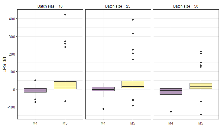
Figure 5.3 displays boxplots of the LPS difference of the selected dynamic model and the static model. The average LPS difference between the selected dynamic model and the static model is around zero, which again shows that the dynamic model does not overfit on static data. On the other hand, for the two dynamic data generating processes, the dynamic model clearly outperforms the static model. Also, one can note that the data partition has minimal effect as there is not much variation in the LPS differences for the different batch partitions.
5.4 Efficiency of the linear Bayes proposal
The efficiency of particle filter algorithms is generally assessed based on the effective sample size
where are the importance weights computed at interval .
To assess the performance of the linear Bayes proposal strategy, we compare it with the local linearisation proposal strategy (Doucet et al. 2000); the state-of-the-art method of constructing proposal densities which approximates the target density (3.2) by a linear Gaussian distribution obtained from a second order Taylor expansion of the target density with respect to the regression coefficients , for . The main difference between these two methods is that the local linearisation method approximates the target density by a Gaussian density without the intermediate step of updating the linear predictors.
Figure 5.4 compares the effective sample size per second generated by the two strategies as a way of comparing their efficiency and computation time. The results are based on data simulated from and a posterior distribution approximated by particles and . The figure shows that the linear Bayes proposal generates an effective sample size that is on average higher than the local linearisation. Both methods are quite fast; their computation time on a simple windows laptop with intel core processor is less than CPU minutes.

6 Conclusions
We introduce a general class of dynamic mixture of experts models for online predictions; the model allows the regression coefficients in each mixture component and weight to vary over time. The component models can be essentially any density function, not necessarily limited to the exponential family.
We propose an efficient SMC algorithm for sequential inference and online prediction that is tailored to handle the proposed model class with potentially high-dimensional parameter spaces. The algorithm handles models with static and dynamic parameters in a unified way.
The model is applied to online prediction of the number of faults in a continuously upgraded large-scale industrial software project. We show that allowing the parameters to evolve over time greatly improves the model’s predictive performance. A simulation study documents that the proposed model selection procedure is i) effective in reducing flexibility when data comes from a static single-component model, ii) able to fit data from multi-component models with time-varying parameters, and iii) it is fast and generates an effective sample size rate that is superior to the state-of-the-art particle filter which uses a proposal density designed via the local linearization of the target density.
References
- Andrieu et al. (2010) Andrieu, C., A. Doucet, and R. Holenstein (2010). Particle Markov chain Monte Carlo methods. Journal of the Royal Statistical Society: Series B (Statistical Methodology) 72(3), 269–342.
- Baydin et al. (2018) Baydin, A. G., B. A. Pearlmutter, A. A. Radul, and J. M. Siskind (2018). Automatic differentiation in machine learning: a survey. Journal of Marchine Learning Research 18, 1–43.
- Bishop (2006) Bishop, C. M. (2006). Pattern recognition and machine learning. Springer.
- Carpenter et al. (1999) Carpenter, J., P. Clifford, and P. Fearnhead (1999). Improved particle filter for nonlinear problems. IEE Proceedings-Radar, Sonar and Navigation 146(1), 2–7.
- Carvalho and Tanner (2005a) Carvalho, A. X. and M. A. Tanner (2005a). Mixtures-of-experts of autoregressive time series: asymptotic normality and model specification. IEEE Transactions on Neural Networks 16(1), 39–56.
- Carvalho and Tanner (2005b) Carvalho, A. X. and M. A. Tanner (2005b). Modeling nonlinear time series with local mixtures of generalized linear models. Canadian Journal of Statistics 33(1), 97–113.
- Carvalho and Tanner (2007) Carvalho, A. X. and M. A. Tanner (2007). Modelling nonlinear count time series with local mixtures of Poisson autoregressions. Computational statistics & data analysis 51(11), 5266–5294.
- Carvalho et al. (2010) Carvalho, C. M., H. F. Lopes, N. G. Polson, and M. A. Taddy (2010). Particle learning for general mixtures. Bayesian Analysis 5(4), 709–740.
- Celeux et al. (2019) Celeux, G., S. Frühwirth-Schnatter, and C. P. Robert (2019). Model selection for mixture models–perspectives and strategies. In Handbook of mixture analysis, pp. 117–154. Chapman and Hall/CRC.
- Chopin (2004) Chopin, N. (2004). Central limit theorem for sequential monte carlo methods and its application to bayesian inference. The Annals of Statistics 32(6), 2385–2411.
- Chopin et al. (2013) Chopin, N., P. E. Jacob, and O. Papaspiliopoulos (2013). SMC2: an efficient algorithm for sequential analysis of state space models. Journal of the Royal Statistical Society: Series B (Statistical Methodology) 75(3), 397–426.
- Del Moral et al. (2006) Del Moral, P., A. Doucet, and A. Jasra (2006). Sequential Monte Carlo samplers. Journal of the Royal Statistical Society: Series B (Statistical Methodology) 68(3), 411–436.
- Dempster et al. (1977) Dempster, A. P., N. M. Laird, and D. B. Rubin (1977). Maximum likelihood from incomplete data via the em algorithm. Journal of the Royal Statistical Society: Series B (Methodological) 39(1), 1–22.
- Douc and Cappé (2005) Douc, R. and O. Cappé (2005). Comparison of resampling schemes for particle filtering. In Image and Signal Processing and Analysis, 2005. ISPA 2005. Proceedings of the 4th International Symposium on, pp. 64–69. IEEE.
- Doucet et al. (2006) Doucet, A., M. Briers, and S. Sénécal (2006). Efficient block sampling strategies for sequential Monte Carlo methods. Journal of Computational and Graphical Statistics 15(3), 693–711.
- Doucet et al. (2001) Doucet, A., N. De Freitas, N. J. Gordon, et al. (2001). Sequential Monte Carlo methods in practice, Volume 1. Springer.
- Doucet et al. (2000) Doucet, A., S. Godsill, and C. Andrieu (2000). On sequential Monte Carlo sampling methods for Bayesian filtering. Statistics and computing 10(3), 197–208.
- Doucet and Johansen (2009) Doucet, A. and A. M. Johansen (2009). A tutorial on particle filtering and smoothing: Fifteen years later. Handbook of nonlinear filtering 12(656-704), 3.
- Fahrmeir and Kneib (2011) Fahrmeir, L. and T. Kneib (2011). Bayesian smoothing and regression for longitudinal, spatial and event history data. Oxford University Press.
- Fahrmeir et al. (2004) Fahrmeir, L., T. Kneib, and S. Lang (2004). Penalized structured additive regression for space-time data: a Bayesian perspective. Statistica Sinica, 731–761.
- Famoye and Singh (2006) Famoye, F. and K. P. Singh (2006). Zero-inflated generalized poisson regression model with an application to domestic violence data. Journal of Data Science 4(1), 117–130.
- Fearnhead and Clifford (2003) Fearnhead, P. and P. Clifford (2003). On-line inference for hidden Markov models via particle filters. Journal of the Royal Statistical Society: Series B (Statistical Methodology) 65(4), 887–899.
- Gamerman (1991) Gamerman, D. (1991). Dynamic Bayesian models for survival data. Journal of the Royal Statistical Society: Series C (Applied Statistics) 40(1), 63–79.
- Gamerman (1998) Gamerman, D. (1998). Markov chain Monte Carlo for dynamic generalised linear models. Biometrika 85(1), 215–227.
- Geweke (1989) Geweke, J. (1989). Bayesian inference in econometric models using monte carlo integration. Econometrica: Journal of the Econometric Society, 1317–1339.
- Geweke (2007) Geweke, J. (2007). Interpretation and inference in mixture models: Simple mcmc works. Computational Statistics & Data Analysis 51(7), 3529–3550.
- Geweke and Keane (2007) Geweke, J. and M. Keane (2007). Smoothly mixing regressions. Journal of Econometrics 138(1), 252–290.
- Goldstein and Wooff (2007) Goldstein, M. and D. Wooff (2007). Bayes linear statistics: Theory and methods, Volume 716. John Wiley & Sons.
- Gordon et al. (1993) Gordon, N. J., D. J. Salmond, and A. F. Smith (1993). Novel approach to nonlinear/non-gaussian Bayesian state estimation. In IEE Proceedings F (Radar and Signal Processing), Volume 140, pp. 107–113. IET.
- Gormley and Frühwirth-Schnatter (2018) Gormley, I. C. and S. Frühwirth-Schnatter (2018). Mixtures of experts models. arXiv preprint arXiv:1806.08200.
- Hastie and Tibshirani (1993) Hastie, T. and R. Tibshirani (1993). Varying-coefficient models. Journal of the Royal Statistical Society: Series B (Methodological) 55(4), 757–779.
- Hjort et al. (2010) Hjort, N. L., C. Holmes, P. Müller, and S. G. Walker (2010). Bayesian nonparametrics, Volume 28. Cambridge University Press.
- Hunter and Young (2012) Hunter, D. R. and D. S. Young (2012). Semiparametric mixtures of regressions. Journal of Nonparametric Statistics 24(1), 19–38.
- Jacobs et al. (1997) Jacobs, R. A., F. Peng, and M. A. Tanner (1997). A Bayesian approach to model selection in hierarchical mixtures-of-experts architectures. Neural Networks 10(2), 231–241.
- Jiang and Tanner (1999) Jiang, W. and M. A. Tanner (1999). On the identifiability of mixtures-of-experts. Neural Networks 12(9), 1253–1258.
- Jordan and Jacobs (1994) Jordan, M. I. and R. A. Jacobs (1994). Hierarchical mixtures of experts and the EM algorithm. Neural computation 6(2), 181–214.
- Klaas et al. (2005) Klaas, M., N. De Freitas, and A. Doucet (2005). Toward practical N2 Monte Carlo: The marginal particle filter. Proceedings of the Twenty-First Conference on Uncertainty in Artificial Intelligence (UAI2005).
- Kohlmorgen et al. (2000) Kohlmorgen, J., K.-R. Müller, J. Rittweger, and K. Pawelzik (2000). Identification of nonstationary dynamics in physiological recordings. Biological Cybernetics 83(1), 73–84.
- Lang et al. (2002) Lang, S., E.-M. Fronk, and L. Fahrmeir (2002). Function estimation with locally adaptive dynamic models. Computational Statistics 17, 479–499.
- Liehr et al. (1999) Liehr, S., K. Pawelzik, J. Kohlmorgen, and K. R. Müller (1999). Hidden markov mixtures of experts with an application to eeg recordings from sleep. Theory in Biosciences 118(3-4), 246–260.
- Liu and West (2001) Liu, J. and M. West (2001). Combined parameter and state estimation in simulation-based filtering. In Sequential Monte Carlo methods in practice, pp. 197–223. Springer.
- Liu and Chen (1998) Liu, J. S. and R. Chen (1998). Sequential Monte Carlo methods for dynamic systems. Journal of the American statistical association 93(443), 1032–1044.
- Malsiner-Walli et al. (2017) Malsiner-Walli, G., S. Frühwirth-Schnatter, and B. Grün (2017). Identifying mixtures of mixtures using bayesian estimation. Journal of Computational and Graphical Statistics 26(2), 285–295.
- Munezero (2021) Munezero, P. (2021). Efficient particle smoothing for bayesian inference in dynamic survival models. Computational Statistics, 1–20.
- Muthén and Shedden (1999) Muthén, B. and K. Shedden (1999). Finite mixture modeling with mixture outcomes using the EM algorithm. Biometrics 55(2), 463–469.
- Pitt and Shephard (1999) Pitt, M. K. and N. Shephard (1999). Filtering via simulation: Auxiliary particle filters. Journal of the American statistical association 94(446), 590–599.
- Quiroz and Villani (2013) Quiroz, M. and M. Villani (2013). Dynamic mixture-of-experts models for longitudinal and discrete-time survival data. Manuscript. https://github.com/mattiasvillani/Papers/raw/master/DynamicMixture.pdf.
- Rasmussen and Ghahramani (2002) Rasmussen, C. E. and Z. Ghahramani (2002). Infinite mixtures of Gaussian process experts. In Advances in neural information processing systems, pp. 881–888.
- Ravines et al. (2007) Ravines, R. R., H. S. Migon, and A. Schmidt (2007). An efficient sampling scheme for dynamic generalized models. Relatório Técnico 201, 2007.
- Richardson and Green (1997) Richardson, S. and P. J. Green (1997). On bayesian analysis of mixtures with an unknown number of components (with discussion). Journal of the Royal Statistical Society: series B (statistical methodology) 59(4), 731–792.
- Rue and Held (2005) Rue, H. and L. Held (2005). Gaussian Markov random fields: Theory and applications. CRC press.
- Stephens (2000) Stephens, M. (2000). Dealing with label switching in mixture models. Journal of the Royal Statistical Society: Series B (Statistical Methodology) 62(4), 795–809.
- Villani et al. (2009) Villani, M., R. Kohn, and P. Giordani (2009). Regression density estimation using smooth adaptive Gaussian mixtures. Journal of Econometrics 153(2), 155–173.
- Villani et al. (2012) Villani, M., R. Kohn, and D. J. Nott (2012). Generalized smooth finite mixtures. Journal of Econometrics 171(2), 121–133.
- Wang et al. (2003) Wang, X., P. Whigham, D. Deng, and M. Purvis (2003). Time-line hidden markov experts for time series prediction. In International Conference on Neural Networks and Signal Processing, 2003. Proceedings of the 2003, Volume 1, pp. 786–789. IEEE.
- West et al. (1985) West, M., P. J. Harrison, and H. S. Migon (1985). Dynamic generalized linear models and Bayesian forecasting. Journal of the American Statistical Association 80(389), 73–83.
- Wood et al. (2002) Wood, S. A., W. Jiang, and M. Tanner (2002). Bayesian mixture of splines for spatially adaptive nonparametric regression. Biometrika 89(3), 513–528.
- Yuksel et al. (2012) Yuksel, S. E., J. N. Wilson, and P. D. Gader (2012). Twenty years of mixture of experts. IEEE transactions on neural networks and learning systems 23(8), 1177–1193.
- Zeevi et al. (1996) Zeevi, A., R. Meir, and R. Adler (1996). Time series prediction using mixtures of experts. Advances in neural information processing systems 9.
Appendix A Gradient and Hessian for dynamic mixture of experts models
A.1 Gradient and Hessian for general dynamic mixture of experts models
This section provides details on the expressions of the gradient and the Hessian of the model (2.1) discussed in Section 3.2. Let as in Section 3.2, the gradient
since , we have
Hence,
The Hessian is
where
It can easily be shown that the first term in the expression above is zero; hence
A.2 Poisson experts
This appendix provides details on the mixture of experts model with Poisson components fitted to the software reports data. The mixture of experts model with Poisson components for the batch , , has the form
To compute the gradient and Hessian required in the proposal density, we define (omitting the index )
The first derivatives are
and the second derivatives are
A.3 Generalized Poisson experts
This section delineates the one-component dynamic generalized Poisson model fitted in Section 4. To simplify the notation we omit the batch index . The generalized Poisson model is of the form (Famoye and Singh 2006)
| (A.1) |
where is the mean and is the overdispersion parameter. The mean and the dispersion parameters are connected to covariates via a log links and respectively.
Let , the first derivatives are
and the second derivatives are
Appendix B Identifiability
Jiang and Tanner 1999 prove that mixtures of generalized linear model experts are identifiable if four conditions hold: i) the experts are irreducible, i.e. no pair of experts have identical parameters; ii) there is an ordering of the parameters to avoid so-called label switching of components; iii) the parameters in mixing functions are set to zero for one of the components; and iv) a certain nondegeneracy condition holds that precludes exact linear combinations of the expert densities. The first condition can be assumed to always hold, otherwise we can just collapse identical experts to a single one and reduce the number of mixture components (Jiang and Tanner 1999). Condition ii) is rarely explicitly imposed in mixture models since it complicates inference, and unrestricted inference will therefore returns one of the identical modes; this is acknowledged in Jiang and Tanner 1999 who recommend in Remark 1 to report the mode corresponding to the order restricted parameters for interpretation. Condition iii) is explicitly imposed in our models by zero restrictions, as is commonly done in mixture of experts models. Condition iv) is a technical condition that should be checked for each distributional family on a case by case basis, but is instead often silently assumed to hold. Jiang and Tanner 1999 prove that several commonly used distributions satisfy the nondegeneracy condition, including the Poisson. In fact, only for binomial experts with the number trials smaller than do Jiang and Tanner 1999 find that the nondegeneracy does not hold, and even then they conjecture that it will hold "for almost all parameters".
Jiang and Tanner 1999 prove their results for generalized linear regression (GLM) components, i.e. for densities in the one-parameter exponential family with a scalar dispersion parameter. However, their proofs only rely on properties of the translation and permutation groups acting on densities, and do not use specific properties of exponential families. Their results therefore also apply to a mixture of GLM-type experts with a single parameter depending covariates, but with a density that may be outside of the exponential family; an example of such a model is the generalized Poisson regression where the mean depends on covariates via a linear predictor through a link function, and the overdispersion parameter is a constant. We will now show that this model satisfies the nondegeneracy condition and a mixture of such experts is therefore identified. For the more general model used in Villani et al. 2012 and in Section 4, where the overdispersion parameter is also allowed to depend on covariates, the issue of identification is not yet resolved. We conjecture however that this model is also identified based on the discussion in the previous paragraph and on the empirical results in Villani et al. 2012 where no convergence issues were encountered when using that model.
To prove that a mixture of generalized Poisson regression experts satisfies the nondegeneracy condition we follow the same technique as in the proof of Lemma 3(a) in Jiang and Tanner 1999 for the identifiability of mixture of Poisson experts. The nondegeneracy condition (Condition 1 in Jiang and Tanner 1999) is that are linearly independent functions of for any distinct pairs , i.e. that
| (B.1) |
only for . Now, if then
| (B.2) |
We can write
| (B.3) |
where and . Now, as the expression in (B.3) behaves as where and . Similar to the proof of Lemma 3(a) in Jiang and Tanner 1999 we therefore have that as the decay/explosion rates of are different for each since the and/or are different. Hence since the equality in (B.1) needs to hold for all , this can only be true for . The mixture of generalized poisson experts therefore satifies the nondegeneracy condition.