Federated Feature Selection for Cyber-Physical Systems of Systems
Abstract
Autonomous vehicles (AVs) generate a massive amount of multi-modal data that once collected and processed through Machine Learning algorithms, enable AI-based services at the Edge. In fact, not all these data contain valuable, and informative content but only a subset of the relative attributes should be exploited at the Edge. Therefore, enabling AVs to locally extract such a subset is of utmost importance to limit computation and communication workloads. Achieving a consistent subset of data in a distributed manner imposes the AVs to cooperate in finding an agreement on what attributes should be sent to the Edge. In this work, we address such a problem by proposing a federated feature selection algorithm where all the AVs collaborate to filter out, iteratively, the redundant or irrelevant attributes in a distributed manner, without any exchange of raw data. This solution builds on two components: a Mutual-Information-based feature selection algorithm run by the AVs and a novel aggregation function based on the Bayes theorem executed on the Edge. Our federated feature selection algorithm provably converges to a solution in a finite number of steps. Such an algorithm has been tested on two reference datasets: MAV with images and inertial measurements of a monitored vehicle, WESAD with a collection of samples from biophysical sensors to monitor a relative passenger. The numerical results show that the fleet finds a consensus with both the datasets on the minimum achievable subset of features, i.e., 24 out of 2166 (99%) in MAV and 4 out of 8 (50%) in WESAD, preserving the informative content of data.
Index Terms:
Internet of Things, Autonomous System, Human State Monitoring, Feature Selection, Machine Learning, Federated Learning, Artificial Intelligence.I Introduction
Automation enables a CPSoS (CPSoS) to run with a minimum human assistance and evolves into autonomy when the human is taken out of the sensing, decision, and actuation loop. Automation can be used to operate a CPSoS comprising complex, dynamic, virtual and physical resources, such as telecommunication networks, computing units, software, sensors, and machines [1]. Humans can interact with an autonomous system either as passive end-users (such as passengers in autonomous transportation system) or rather as active co-operators in a mutual empowerment relationship towards a shared goal. Such cooperative, connected, and autonomous systems have the potential to be a game-changer in multiple domains if they will be capable of positively exploiting such an inescapable human factor. The increasing development of semi-ADS poses the challenge of taking the end-user, in the middle of the evolution process toward fully ADS. Aside from vehicle control, a CPSoS needs to monitor the comfort/discomfort of the passenger, as well, to improve its well-being and to acknowledges the degree of safety and satisfaction perceived about the ADS. AI (AI) is a fundamental technology for deploying the future CPSoS for ADS [2]. The stringent computational and memory requirements for ML (ML) algorithms will impose a significant rethinking of the underlying computing and communication system and will have to fit the constraints of the onboard units. Information extraction should follow as much as possible optimal criteria, cooperating with the inherently distributed nature of the automotive scenario.
Moreover, local processing of information can also be an advantage in specific scenarios with intermittent connectivity or when data privacy is a key issue [3]. Hence, reducing the transfer time needed of either raw data or the relative features is of the utmost importance in determining the performance of computation offloading. Intuitively, traditional data compression techniques [4] could reduce such a delay component, but will also degrade the relative classification performance [5], prolonging the training phases as well as degrading the inference performance.
Conversely, when information extraction algorithms produce massive streams of features, selecting the most relevant ones to feed a ML model becomes very convenient, both in terms of compression and accuracy preservation. Such an operation is known as FS (FS) [6] and allows for achieving simpler and, therefore, more efficient ML-based models [7].
This work focuses on feature selection efficiency within a fleet of AV, which collect, through their sensors, multi-modal raw measurements to be pre-processed and delivered to feed a remote edge server for inference tasks. Such a procedure can introduce information redundancy, which leads to a waste of computing and communication resources. The AV ensemble aims at limiting the transmission to the top relevant features only. However, just a subset of the top ones can be extracted from each local data collection in a distributed manner w.r.t. the whole set achievable from the union of the local datasets but in a centralized manner. In fact, the former case may lead to an inconsistent model w.r.t. to the latter. Therefore, the AV, shall participate to a collaborative FS process, in order to exploit the whole information in a federated manner. We tackle this problem, by proposing, for the first time, a FFS (FFS) algorithm, exploiting a distributed computing paradigm applied to AV. In FFS all AV collaborate to come up with the minimal set of features selected from their local datasets.

The proposed FFS system is made up of two components provided in Figure 1:
- •
- •
An aggregation algorithm executed on the ES (ES) that combines the local estimates received from the AV. The aggregation algorithm is based on a Bayesian approach to merge the local information into a global one.
The messages delivered by AV contain probability vectors where each element is the probability to select that feature. The ES returns the ”federated” probability vector which is derived by the aggregation of the vectors received by the AV, as detailed in the following, to replace each of the local ones. Note that, the proposed approach does not need to share any local raw data but only the estimates of the local most informative features. Moreover, it guarantees that all the AV reach a consensus on the subset of the most informative features, after a finite number of communication rounds, i.e., the messages exchanged between the AV and the ES.
As we show in the paper, the proposed algorithm (i) significantly limits the control messages exchanged during the FFS process and (ii) provably let the AV converge to a subset of top features, which effectively reduce the information stored and transmitted by the AV. Specifically, numerical results show that, on reference benchmarks, our solution limits data processing and transmission, by removing up the to 99% of redundant features from the selected datasets, without loss of accuracy on the learning model.
Summarising, the novel contributions of this paper are:
- •
A novel FFS algorithm based on the MI CE (client-side) on the AV and a Bayesian aggregation approach on the ES.
- •
The theoretical proof that such an algorithm converges to a stable solution in a fixed number of iterations.
- •
An extensive numerical evaluation tested on two real-world datasets that shows the efficiency of our solution.
The paper is organized as follows: related works are presented in Section II; the reference scenario and the system assumptions are presented in Section III; the theoretical background underlying the proposed feature selection approach is presented in Section IV; the federated version of the feature selection algorithm in presented in Section V; Section VI presents the experimental results of a study case with two real world datasets, belonging to different application domains; conclusions in Section VII.
II Related Works
II-A Feature Selection
Many FS procedures have been proposed in the literature. In [11, 12, 6] authors provide a comprehensive overview of the existing methods. Additionally, they consider the most important application domains and review comparative studies on feature selection therein, in order to investigate, which methods outperform for specific tasks. Authors highlight that FS is based on the identification of the relevance and redundancy provided by the features with respect to a class attribute function. The main approaches of FS fall into three categories: filtering, wrapping, and embedded methods. This categorisation is based on the interaction between the selected features and the learning model adopted to take a decision. The output of the wrapping and embedded methods is tightly connected to the learning model that uses the selection. Therefore, with these methods FS and model training cannot be uncoupled. Conversely, filtering methods are suitable for being used regardless the presence of a learning model to train.
As shown in [11, 12, 6], most of the well-known filtering algorithms use information-based metrics for FS, and can deal with samples of variable lengths, as presented in [13, 14]. A suitable information-based metric for the FS is the MI. MI has gained increasing popularity in data mining, for its ease to use, effectiveness, and strong theoretical foundation. mRMR [15] and HJMI [16] are some of the most used methods that exploit MI. These approaches rank the features according to the maximization of the MI and let the user to select a desired subset . Differently, the proposed algorithm automatically select a minimal subset of relevant features, also capturing the mutual dependencies. Note that the formulation of the underlying optimization problem is NP-Hard[8, 9], i.e., MI-based feature selection problem involves the integer programming or, in some cases, the quadratic integer programming. In [17, 18, 19] authors show how to adopt the CE approach to address such native computational complex problems, for different application scenarios. Beyond MI, other filtering methods can use different metrics, such as in [20] where the authors evaluate the variance of all the features to measure the impact that each of them has on the learning process. This method relies on the concept that the features with zero variance add no information, by considering the relation between the target variable and feature vectors.
To the best of our knowledge, all these algorithms are designed for being executed in a centralised setting, i.e., under the assumption that the whole dataset is available to the learning agent.
II-B Distributed Learning
Distributed learning is considered from several perspectives in the literature. A very consistent body of work deals with distributed learning based on the FL (FL) framework. FL is a distributed learning framework initially proposed by Google, where a large number of mobile or edge devices participate in a collective and distributed training of a shared model. [21, 22]. FL is an iterative procedure spanning over several communication rounds until the convergence is reached. Based on this paradigm, several modifications have been proposed concerning (i) new distributed optimisation algorithms [23, 24, 25, 26], and (ii) privacy-preserving methods for FL [27, 28]. Alternatively, other approaches do not rely on a centralised coordinating server. In [29, 30], authors propose a distributed and decentralised learning approach based on Hypothesis Transfer Learning. Similarly to the FL framework, authors assume that several devices hold a portion of a dataset to be analysed by some distributed machine learning algorithms. The aim of [29, 30] is to provide a learning procedure able to train, in a decentralised way, an accurate model while limiting the network traffic generated by the learning process. The vast majority of the distributed learning solutions, presented in the literature, focus on the model’s training, giving the feature engineering phase for granted. Until now, the idea of performing FS, directly, on edge devices remains unexplored.
In the literature only few approaches cope with FS in distributed settings. In [31], authors present a distributed algorithm for FS based on the Intermediate Representation, which aims at preserving the privacy of data, allowing the node to exchange each other the data they hold. Therefore, in this method FS is performed under the assumption that all data are available to the FS algorithm. Moreover, the method presented by the author depends from the specific learning model that uses the selected features.
In [32], the authors propose an information-theoretic FFS approach called Fed-FiS. Fed-FiS estimates feature-feature mutual information and feature-class mutual information to generate a local feature subset in each user device. Then a central server ranks each feature and generates a global dominant feature subset using a classification approach. This approach has some commonalities with ours, such as the adopted metric (MI) and the federated settings. However, differently from [32] (i) we provide directly the minimum set of relevant features instead of a ranking, (ii) we propose an aggregation based on Bayes’ theorem that does not rely on any Machine Learning scheme to finalise the selection (i.e., no regression or classification methods are adopted in our solution), resulting in a computationally more suitable approach for vehicular scenarios.
In light of this and to the best of our knowledge, this is the first paper that proposes a federated mechanism of feature selection explicitly designed to meet the requirements of the CPSoS context.
III System assumptions
In this section, we describe the reference scenario and the system assumptions considered in this paper. As shown in Figure 2, we consider a set of AV, implementing an ADS each, collecting data generated by the sensors integrated in a CPSoS and that collaborates with the others ADS to learn a minimal, and most informative set of features from their local datasets. To this end, the AV execute an in-network data filtering process through our FFS approach to reach a consensus in identifying the most informative feature subset. Finally, the globally shared feature set is used like a compression scheme before transmitting it to an ES. Note that, in this system the AV are only responsible for finding the best compression scheme applicable to the their local data in a collaborative way, based only on the control information they exchange with the ES. Moreover, the ES has a three-fold role: i) it acts as central coordinating entity in the FFS process whose purpose is to aggregate the partial control information sent by the AV; ii) it acts as final collector for the compressed data, once the FFS is completed and, iii) runs the AI services to extract knowledge from data but that is used only for performance evaluation in this paper. We target two different user cases to validate the performance of the proposed FFS method. The former refers to the localization of an AV in the environment based on images and inertial measurements, and the latter regards the physiological-state monitoring of a passenger in the automotive domain. We define two different sub-systems part of the same CPSoS: the ADS of above, and an HSMS (HSMS) to learn the feeling perceived from a passenger relatively to the ADS driving style. Therefore, we assume each AV to be equipped with a camera to capture images from the surrounding environment aside some inertial sensors for the former learning task, and a set of body sensors, such as, ECG (ECG), EDA (EDA), EMG (EMG), and RSP (RSP) for the latter.
Each AV is able to locally synchronize the multi-sensory data such that, for each image, it is possible to associate the corresponding inertial measurements leading to an enhanced Raw Input Datum (eRID). Note that for the scope of this paper it is not important the specific semantic of the labelling, but it is enough to assume a labelling process on the collected data. The AV are also equipped with a relatively small edge computing unit (e.g., a RaspeberryPi or, at most, an Nvidia Jetson Nano) able to cache data and execute the FS task, before transmitting the features. Additionally, the AV are endowed with a radio communication interface to communicate toward the ES. It must be noted that the task is not collecting images of the environment, or physiological parameters of the user but, conversely, retrieving the information associated to those images or to those physiological sensors, e,g., the position of the AV with respect to the surrounding or the user mood. In particular, the latter is labelled according to the classification scale provided by questionnaires like PANAS, SSSQ or SAM [33], which associates numerical labels to the physiological states.

IV Feature selection
In this section, we provide the theoretical background of the MI-based FS algorithm and the relative implementation based on the CE method.
IV-A Background feature selection based on Mutual Information
To make the paper self-contained, we report in this Section the necessary theoretical background needed to get an intuition about the internal details of the CE-based FS method presented in Section IV-B.
First, let us define the FS problem as follows:
Definition (FS Problem).
Given the input data matrix composed by samples of features (), and the target attributes’ (or labels) vector , the FS problem is to find a -dimensional subset with , by which we can characterize .
The method we adopt in the paper performs the FS measuring, through the Mutual Information metric, the amount of information that a subset of features (or attributes) expresses with respect to a specific target label .
| (1) |
where , and is the conditional entropy which measures the amount of information needed to describe , conditioned by the information carried by . Hence, represents the dependence between and , i.e., the greater the value of , the greater the information carried by on . We recall that the MI between two random variables and is strictly related to the entropy , which defines the amount of information held by the variables, i.e., the entropy of a random variable (i.e., ) and its probability are inversely proportional: the greater the entropy of a random variable , the greater its unpredictability and vice-versa. Hence, we can assert that the entropy measures the diversity of in terms of the uncertainty of its outcomes.
In MI-based FS the features to be selected are those that maximise Equation (1). These features are typically referred as EA (EA). By solving the following optimization problem we would obtain the optimal global solution to the FS problem defined in Definition:
| (2) | |||
Note that the problem (2) belongs to the class of Integer Programming (IP) optimization problems and finding its optimal solution is NP-hard [36], i.e., the optimal solution would be found among all combinations of feature indices of the native set .
The problem (2) becomes computationally tractable if approached through an iterative algorithm which selects and adds to the subset one feature at a time. Therefore, instead of solving 2, we address the problem defined in (3):
| (3) | |||
For the sake of clarity, we provide an intuitive example based on the relation between MI and the entropy. Considering Figure 3, the circles are the entropy of the random variables , and the grey regions are the information carried by the variable (or ) on . The dashed area shows the information redundancy of the variable (or ) given the already selected variables in . In this example, the variable should be added to the set since it is more informative than on , i.e., its grey area is larger than ’s, and it is less redundant than w.r.t. to .
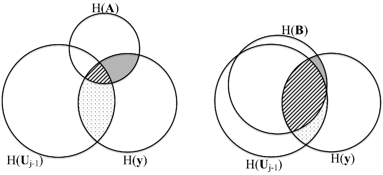
The main drawback of this approach is that it might end up with a sub-optimal solution because, by selecting the features one by one, the algorithm makes the implicit assumption that they are independent, which might not hold true. Theoretical foundations for the incremental version of the FS algorithms has been proven by the authors in [35, 34]. It is worth mentioning that a connected issue with problem (3) regards the efficient evaluation of the MI, which might become prohibitive even for datasets with a small number of samples. We overcome this problem by adopting the MIToolbox [37], a state-of-the-art tool for numerical optimization.
IV-B CE-based feature selection algorithm
In this section, we describe the CE-based algorithm that finds, in a finite number of steps, a solution that well approximates the one found by solving problem (2), while making negligible the assumption of independence among features introduced in problem (3). In other words, with CE-based FS, instead of selecting one EA at a time, we select a set of EA jointly.
The CE-based algorithm is based on the following intuition: if the set contains only EA, then , which implies that [35, 34]. Note that with our approach, we avoid the greedy research of the set among all the possible solutions which realizes . Instead, we adopt the stochastic approach. Precisely, we associate each -th feature with a random variable . The CE-based algorithm identifies which variables must have , so that the objective function gets close to . This is called ASP (ASP) [10]. In this way, we get the optimal distribution of the binary vector through which we identify the features to be selected, i.e. the -th feature is selected if . It is worth noting that searching for the solution of the optimization problem through the definition of the ASP has the advantage of addressing the native problem in (2) as a convex problem.11 1 More details are in Section 4 of [10].
We formulate the ASP as a minimization problem, as shown in Eq. 5. In the following we present the essential steps that brings to its formulation. Briefly, we need to find the probability distribution of the values in equal to that solves the equation:
| (4) |
where is the indicator function of the event , and is the minimum value for our objective function. Precisely, at step t is calculated as the percentile of the objective function calculated by using the samples drawn from the distribution at step t. Note that, the authors in [10] recommend to set in the range . The indicator function is equal to for all the possible configurations in that verify the event , and otherwise.
We estimate through the Likelihood Ratio (LR) estimator with reference parameter . Precisely, we apply the LR theory of estimation [10] to define the following optimization problem and to obtain the optimal value for the distribution.
| (5) |
where is a set of possible samples drawn from the distribution .
As stated above is a vector of independent Bernoulli random variables where takes value equal to with probability and with probability . Hence, can be written as:
| (6) |
Given that the objective function of problem (5) is concave22 2 The logarithm is a concave function, the indicator function is or so the weighted sum of concave functions gives still a concave function., we can solve it in closed form by imposing:
leading to:
| (7) |
In the CE-base algorithm the result in the equation (7) is used for updating the distribution as follows:
| (8) |
The mathematical analysis about the choice of the parameter is provided in the Appendix-A of this work. Further indications on the choice of can be found in [10, 38, 39]. The derivation of equations (5-7), as well as, the optimality of are proven in [10].
The solution of the problem defined in (5) is achieved through Algorithm 1: it starts with an initial guess of ; Bernoulli random samples of size each (line 4) are drawn at each step . For each sample , the values of the conditional entropy (line 7) are computed on the dataset where the only active features are those corresponding to the elements equal to one (line 6) in . The subset selection is shown in the procedure (lines 15-26). Then we compute (lines 9-10) as in Eq. (7) and finally we update the current estimate of the probability vector (line 11) as in Eq. (8).
V Federated Feature Selection
In this section we present how we exploit the CE-based FS algorithm presented in Section IV and summarised in Algorithm 1 to design our FFS algorithm FFS, described in Algorithms 2 and 3. They cover, respectively, the two functional blocks of FFS, i.e., Algorithm 2 is executed by the ES to coordinate the distributed FS and Algorithm 3 runs on the clients. The FFS is an iterative procedure. At the beginning, the ES sends to the clients involved in the process a vector where each element represents the probability that each feature has to be selected according to its importance (lines 8-10 of Alg.2). Each element of is initialized to , i.e., this is a common choice when using the CE algorithm. The vector represents a piece of global information that the ES shares with the client nodes. Each client uses to initialize its local copy of the probability vector, i.e., and runs the local FS procedure based on its local data (lines 2-3 of Alg. 3). At the end of the local FS, the -th client sends to the ES the locally updated probability vector and a control information regarding the cardinality of its local data whose purpose will become clear in the following. The ES computes the new global probability vector (line 13 of Alg. 2) by aggregating the ones received from the clients as expressed in Equation (9) and discussed later on. The updated vector is transmitted to the nodes that run Algorithm 3 by updating the local probability vector with the new global one. This procedure iterates until the distribution global probability vector converges to a stable one. In FFS we check convergence by comparing the distribution of the current global probability vector to the previous one using the Kolmogov-Smirnov statistical test for two one-dimensional samples (KS-test). The procedure stops when (i) the p-value of the KS-test is greater than a fixed threshold33 3 We empirically observed that the closer to one, the more accurate the solution. and, (ii) its variation from the previous one is less than (line 7 of Alg. 2).
The core point of Algorithm 2 regards the aggregation step (line 13 of Alg. 2) where the ES merges the local probability vectors into the global one which, in our solution, is defined as a weighted average. The main idea is to merge the local probability vectors by a weighted average where the weights (computed as in Eq. (10)) serve the twofold purpose of (i) considering more (or less) those vectors that are computed from larger local datasets and (ii) defining a common support among all the probability vectors. This second aspect is quite crucial for the consistency of the computation in Eq. (9).
Formally, we assume that each node acquires a number of i.i.d. records to perform the FS, and that the nodes share the same set of features . The global probability used for the FS can be written as follows:
| (9) |
where is the solution of problem (5) at node obtained by using Algorithm 1, and weights w.r.t. the other nodes, whose formal definition is:
| (10) |
As anticipated, according to equation (10), we weight the probability vector of node proportionally to the size of its local dataset compared to the whole amount of data present in the system. In this way, we can contrast situations where local datasets are heterogeneous w.r.t. the size.
In FFS, the updating scheme can be, at least in principle, both synchronous and asynchronous, provided that the set of nodes involved in the process does not change over time.44 4 Note that this condition does not imply that all nodes must be active during the entire process. In fact, as we will show in Section VI our system is robust to the presence of churning nodes. Precisely, we assume a system where the ES after having sent the updated global probability vector, expects the nodes to receive their local updates within a fixed time slot, after which, it begins the aggregation step using only the information received. Therefore, the number of updates used to compute the new global probability vector might change because a subset of nodes could not communicate their updates within the deadline set by the ES. Regardless of the number of nodes that contributed to the aggregation step during one round of communication, the ES broadcasts the new global probability vector to all nodes in the system. In this way, all nodes start the new round of local computation from the same starting point, and, consequently, we dramatically limit the potentially detrimental effects deriving from the aggregation of outdated local probability vectors. Moreover, as proved by the convergence analysis provided in Appendix-A and Appendix-B, independently from the updating scheme, FFS converges in a finite number of steps to the very same solution as running the CE in centralised settings i.e., with complete access to the entire dataset.
It’s worth noting that our solution is able to cope with feature redundancy in federated settings. Precisely, this represents an issue that might prevent the possibility of performing the FS in federated settings. In fact, running a standalone FS algorithm on different local datasets where there is redundancy between features, different FS might occur but with an equivalent information content across all the AVs. This aspect makes all the local selections completely useless regarding the communication efficiency, due to the consequent lack of agreement on the FS between the AVs. Conversely, since in FFS the AVs share at each communication round their local information, they may come up with a final agreement on the FS. Summarising, even if there is redundancy between features, the final selection is consistent among all the AVs and, according to results presented in Section VI, it is also accurate if compared to the centralized FS (i.e., when all the local raw data are transferred onto the ES).
VI Numerical evaluation
In this section, we present the numerical results of our compression method based on the FFS algorithm presented in Section V. Before going through the results, we introduce the datasets, the simulation settings, the methodology, and the metrics used to evaluate our solution’s performance.
VI-A Dataset description and simulation settings
We based the performance evaluation of FFS on two datasets, each one mapping one of the two use cases described in Section III. The first one called MAV55 5 dataset available at: https://tinyurl.com/mavmr01 is a publicly available dataset containing both 6464 images and IMU collected by a AV during a mission in a controlled environment. The second dataset called WEarable Stress and Affect Detection (WESAD) is a collection of data sampled from heterogeneous biophysical sensors: ECG, EDA, EMG, Temperature, Respiration and Inertial Measurements on the three axes.
MAV dataset
both images and inertial measurements are synchronised to obtain a set of eRIDs. We pre-process the raw images to extract more informative features as it is customary in the computer vision domain. Feature extraction eases the training of a machine learning model and, performs a preliminary step of data compression. In fact, a raw image is made of 4102 floats (6464 pixels + 6 IMU readings) while, after the feature extraction, it shrinks down to a vector of size 2166 floats. In our settings, we extract the HOG (HOG) features66 6 HOG is a standard feature extraction methodology used in computer vision and image processing to create an image descriptor that captures the spatial relations between different portions of it [40]. , and we assume that the feature extraction is accomplished directly on the AV, which might be possible if equipped with a board of the kind discussed in [40]. Note that the original dataset is unlabeled. Therefore we labelled it in a way compatible with the original context of positioning. To this end, we associated with each eRID a label corresponding to the corresponding voxel.77 7 A voxel represents a value on a regular grid in three-dimensional space. Table I shows the structure of an eRID for the MAV; the first 2160 feature are HOG while the last 6 are IMUs, i.e., acceleration (ACC) and angular velocity (AV).
| 0 | 1 | 2 | … | 2158 | … |
|---|---|---|---|---|---|
| HOG # | |||||
| 2160 | 2161 | 2162 | 2163 | 2164 | 2165 |
| ACCx | ACCy | ACCz | AVx | AVy | AVz |
The whole dataset contains 2911 labelled records. To simulate the federated data collection, we split it into disjoint partitions of size 291 records such that each partition is i.i.d. w.r.t. the entire dataset. Each subset represents a AV. The data collection is slotted; hence, the AV draw with replacement a random sample from their local dataset for each time slot. This sample is used to perform the local computation of the distributed algorithm followed by a communication round for synchronising the AV on the local FS. Each random draw’s size is accumulated to trace the cache necessary for storing data until the completion of the distributed FS.
WESAD dataset
it provides data in terms of features and labels already useful to perform the detection of stress and affection state of human subjects. The dataset contains readings from two devices, i.e., Respiban and Empatica E4, positioned i) on the chest and ii) on the wrist of human subjects. Each device is equipped with multiple sensors monitoring several physiological parameters. Since the two devices have different operating settings, we focused on the Respiban, whose collection rate is homogeneous for all its sensors. The dataset contains readings collected from 17 human subjects, which perform a predetermined protocol to induce the body in one of the following states: 0-baseline, 1-amusement, 2-stress, 3-meditation, 4-recovery. The data collected for each subject amounts to 3.6M records, equivalent to 220 MB. A complete description of the dataset is provided in [33]. Table II shows the structure of an eRID for the WESAD.
| 0 | 1 | 2 | 3 | 4 | 5 | 6 | 7 |
|---|---|---|---|---|---|---|---|
| ACCx | ACCy | ACCz | ECG | EMG | EDA | TEMP. | RSP |
Due to the huge size of the dataset we used the data from 5 out of 17 subjects, corresponding to 1.1 GB. The data is already partitioned according the subject ID, thus we keep the original partitions. In our simulated scenario, each partition corresponds to an edge device holding the data of only one subject, i.e., no artificial data re-distribution is performed. As for the previous scenario, each device executes FFS using only its own data.
We evaluate the performance of our methodology according to two metrics:
- •
accuracy: to assess the quality of the distributed FS
- •
network overhead (): to evaluate the impact in terms of network traffic generated by our methodology
Our target is to compress the data to be transmitted, without significantly degrading its informative content.
Accuracy metric
The quality assessment is a two-stage procedure. First, we set the baseline validating the quality of the features selected by CE executed in a centralised setting, i.e., we train a classifier using the set of selected features (CE-CFS) on the entire dataset, and we compare its prediction performance with that of a second classifier trained on the whole set of features (NO-FS). If the CE-CFS performance on a smaller group of features is comparable or equivalent with the one identified by NO-FS, we consider the FS valid. To strengthen this initial evaluation, we compare the centralised results of CE-CFS with other three reference FS algorithms: mRMR[15], HJMI[16] and ANOVA[20]. As we will show in the following, for all these benchmarks we have to specify the size of the features selection. Since we are interested in assessing the quality of the FS and for the sake of fairness, we set equal to the size of the FS obtained by CE-CFS (which finds such a number in a completely autonomous way).
Then, we repeat the same procedure training another classifier on the subset of features obtained from our FFS and we compare its performance with all the centralised methods. We split the dataset in train (80%) and test set (20%). The train set is used for both FS and model training, while the test is used for performance evaluation only. The accuracy is defined as the average of correctly classified records
| (11) |
where N is the size of the test set, is the indicator function, and are the -th predicted and true label, respectively. For the sake of statistical significance, the training is repeated ten times, changing the initialisation of the classifier and the composition of training and test set. The reported results are average values accompanied by confidence intervals at 95%.
Network Overhead
we measure the network traffic generated by our solution as follows. On the one hand, we compute the network overhead generated by the FFS network defined as:
| (12) |
where is the number of communication rounds before all the AV involved in the distributed FS converge to a solution, is the number of nonzero floating point numbers belonging to the probability vector in (9) exchanged between the AV during each round plus the weight in (10). The symbol is the size of the bit map used to reconstruct the position of the non-zero elements exchanged between the AV and the edge server. On the other hand, we compute the compression obtained through the FS as:
| (13) |
where is the selected set, and is the entire set of features.
VI-B Settings the baseline: FS in centralised settings
The following results regard the first stage of the validation, i.e., the accuracy of a classier trained using only the subset of features identified by the CE algorithm w.r.t the performance obtained by a classifier trained on the entire dataset. For this stage of validation, we train a Neural Network (NN). For MAV the NN is a multi-layer perceptron with two hidden layers of 300 and 100 neurons each. For WESAD, we used a deep NN with four hidden layers of 300,100,64,32 neurons each. The input layer’s size depends on the number of features selected, while the size output layer is 37 and 5 for MAV and WESAD, respectively. The activation function is ‘‘ReLU’’88 8 REctified Linear Unit and the optimizer is ‘‘Adam’’99 9 Stochastic Gradient Descent with ADAptive Momentum for both the models. These are very common settings which typically provides good performance [41].
| Dataset | Method | Size | FS | Accuracy | |
|---|---|---|---|---|---|
| (# record) | (#) | (%) | (%) | ||
| MAV | NO-FS | 2911 | 2166 (All) | - | 97.50.4 |
| CE | 2911 | 18 | 99 | 96.70.5 | |
| MRMR | 2911 | k=18 | 99 | 95.00.5 | |
| ANOVA | 2911 | k=18 | 99 | 95.00.4 | |
| HJMI | 2911 | k=18 | 99 | 96.30.7 | |
| WESAD | NO-FS | 15 | 8 (All) | - | 94.30.7 |
| CE | 15 | 4 | 50 | 94.60.8 | |
| MRMR | 15 | k=4 | 50 | 94.30.8 | |
| ANOVA | 15 | k=4 | 50 | 94.50.5 | |
| HJMI | 15 | k=4 | 50 | 90.21.6 |
Results in Table III show that CE algorithm executed on both datasets in centralised settings can autonomously identify a minimal set of features (i.e., 18 for MAV and 4 for WESAD) with the very same informative content of the whole feature set. The accuracy obtained by both the NN models trained on the CE’s FS is statistically equivalent to the one obtained on the whole set of features, inducing a quite impressive compression rate (): up to 99% and 50% of network traffic for MAV and WESAD, respectively. As a further confirmation of the CE results, we perform the FS using other three reference benchmarks, i.e., MRMR, ANOVA, HJMI. Note that all these approaches select a subset of features with the very same informative content of CE. However, we point out that for all of them we have to decide beforehand the number of features to be selected. This represent a major shortcoming that, instead, CE-based methods overcome by design, since the number of features to be selected is a byproduct of the CE algorithm. Finally, these results assess the suitability of the CE algorithm on both datasets, thus we can use them as a benchmark for the evaluation of our distributed FFS method.
VI-C Evaluation of Federated Feature Selection
We focus now on the analysis of our FFS method. We compare its performance to those obtained by CE executed in centralised settings (CE-CFS). We recall that, in federated (distributed) settings, each AV can process only the data it locally collects.
First we assess the performance of FFS in a static distributed scenario where the AV have collected all the data and, before sending them to the ES, they perform the distributed FS in order to transmit only the very necessary information.
| Dataset | Method | Size | FS | Accuracy | |
|---|---|---|---|---|---|
| (# obs.) | (#) | (%) | (%C.I.) | ||
| MAV | CE-CFS | 2911 | 18 | 99 | 96.70.5 |
| FFS | 291 | 24 | 99 | 96.70.4 | |
| WESAD | CE-CFS | 15M | 4 | 50 | 94.60.8 |
| FFS | 3M | 4 | 50 | 94.60.8 |
Table IV reveals that for MAV dataset, FFS finds a set of features that, although slightly larger than that found by CE-CFS (24 instead of 18), it has the very same informative content, i.e., the accuracy of the NN model trained on both subsets of features are statistically equivalent. As we can see, the results also hold for the WESAD dataset. Precisely, FFS selects the same number of features identified by CE-CFS. Specifically, FFS and CE-CFS select the same set, i.e., the features with indexes [1,2,5,6], explaining why the NN achieves the same prediction accuracy. We motivate such an exact correspondence between FFS and CE-CFS selection considering that the small size of the complete feature set of WESAD might prevent a high number of feature subset with equivalent informative content. Such an assumption also holds for the MAV dataset. In fact, as we can see in Figures 5a, 4b FFS and CE-CFS select the same subset of IMU features. Conversely, when the set of features is more redundant, as it is for the HOGs, there might exist several subsets holding the same informative content. The comparison in Figures 5a and 4a confirms such a claim because the two feature sets are overlapping but not equal, yet the overall accuracy is comparable.
This result provides a preliminary insight regarding the effectiveness of the Bayesian aggregation used to merge the information extracted by the AV from their local datasets. Precisely, Figure 6 shows the number of selected features at each communication round for the MAV case. As we can see, in the beginning, the cardinality of FS remains almost constant. In this phase, due to the partitioning of data in separated datasets, the CE algorithm has not yet enough knowledge to identify the most informative features. However, the number of features added to the selection starts increasing following an almost-linear trend in a few communication rounds (16). The process ends after 44 rounds, i.e. when the distribution of probabilities indicating the most informative features becomes stable.
| Dataset | Size | FS | Accuracy | Cache | |||
|---|---|---|---|---|---|---|---|
| (# obs) | (#) | (%C.I.) | (#) | (%) | (MB) | (MB) | |
| MAV | 291 | 24 | 96.70.4 | 44 | 99 | 16 | 217 |
| 203 | 26 | 96.50.3 | 37 | 99 | 13 | 128 | |
| 145 | 34 | 97.00.3 | 55 | 98 | 20 | 134 | |
| 87 | 59 | 97.20.3 | 43 | 97 | 15 | 63 | |
| 29 | 41 | 97.20.4 | 53 | 98 | 19 | 26 | |
| WESAD | 3 | 4 | 93.60.8 | 11 | 50 | 0.009 | 2 |
| 1 | 5 | 93.80.5 | 10 | 38 | 0.008 | 1 |
Our method’s capability to converge quickly to the final and most informative set of features directly affects the amount of network traffic generated upon the completion of the FFS. To confirm such a claim, we performed a set of simulation in which we run FFS varying the size of the local dataset available at the edge device. In this way, we want to analyse our method’s robustness when each edge device can access only a limited amount of data. In Table V we report the size of data used for each update (Size), the number of selected features (FS), the accuracy, the number of communication rounds upon convergence (), the compression obtainable with FFS (), the network overhead generated by FFS (), and the size of the cache needed to collect the data before starting the data transmission. Overall, we observe that, for both datasets, decreasing the size of data processed at each round does not affect significantly the number of communication rounds needed by FFS to converge to a solution, which results in limiting the network overhead generated during the process. Specifically, considering a dynamic data collection process as in the MAV-related use case, we see that the network overhead is always i) less than the storage needed to cache the data before starting the transmission and ii) negligible considering the compression achieved (i.e., up to 99%). Interestingly, the same holds also for the WESAD scenario. In this case, the network overhead can be considered negligible w.r.t. the size of the data processed (MB) if compared with the compression rate achieved by FFS (up to 50%).
| Dataset | FS | Accuracy | |||
|---|---|---|---|---|---|
| (#) | (%C.I.) | (#) | (%) | ||
| MAV | 0.2 | 48 | 97.00.4 | 37 | 98 |
| 0.3 | 80 | 97.20.3 | 35 | 96 | |
| WESAD | 0.2 | 4 | 94.50.4 | 9 | 50 |
| 0.3 | 3 | 67.40.4 | 7 | 63 |
| Dataset | Method | Local FS intersection |
|---|---|---|
| (%) | ||
| MAV (k=18) | MRMR | 0 |
| ANOVA | 0 | |
| HJMI | 0 | |
| WESAD (k=4) | MRMR | 100 |
| ANOVA | 100 | |
| HJMI | 100 |
In Table VII we show how the benchmark methods MRMR, ANOVA and HJMI behave when run in isolation on local dataset. Each method has been configured to select the optimal number of features found in a centralised setting. This is clearly an unrealistic situation that we use to demonstrate the limitations coming from running a non-FFS algorithm in federated settings (i.e., on partial datasets). Precisely, taking into account the MAV dataset, all the algorithms run in isolation on each AV, find a different subset of features (i.e., null pairwise intersection). No agreement between AVs on the subset of features means that all the local data must be transmitted to the ES, causing a non negligible waste of network resources. We motivate this behaviour with the fact that the original subset of features is redundant, as in MAV, running the FS in isolation on portions of data is not a winning strategy. Conversely, when the original subset of features is less noisy, as in WESAD, it is more likely that all the AVs find, completely by chance, the same subset of features, i.e., without a way to coordinate the features selection in a consistent and provable way, there are no guarantees for the AVs to identify a consistent and shared subset of features.
Finally we analyse the FFS performance in presence of faulty nodes, i.e., a node experiencing issues in transmitting successfully its updates to the ES. Note that, the causes preventing the updates’ transmission might relate to either communication-related (i.e, a noisy channel) or the presence of a power-saving policy regulating the duty cycle of AV switching off the network interface for a time corresponding to a communication round. The aim is assessing the robustness of FFS when few nodes cannot contribute to the distributed learning at each communication round. To this end, we simulate a scenario where, at each communication round, a random number of AV fail to communicate their updates to the ES. We model the fault of a AV performing a random draw from a Bernoulli distributed random variable, with parameter . At the beginning of the simulation we set and, for each communication round and for each node, we perform a random draw, where 0 means faulty and 1 means non-faulty. This means that the updates of a faulty AV are not considered for the execution of Algorithm 2. We consider a fault rate equal to 0.2 and 0.3, meaning that at each round there are, on average, 2 and 3 faulty AV out of 10, respectively. Such values can be reasonably assumed as upper bounds to evaluate the performance of the system. Higher rates would reveal that the scenario is not reasonably set up to run with any sort of reliability.
In Table VI we report the performance of FFS, for both datasets. For the MAV dataset, although FFS selects and more features than the case when all the AV contribute to the process (see TableIV), the compression rate deteriorates by 1% and 3%, respectively. The quality of the selection is confirmed by the accuracy that is statistically equivalent to the case without faulty AV. Regarding WESAD, we notice that for FFS performance is equivalent to the case with all non-faulty AV. Conversely, for FFS selects a smaller (i.e., 3 instead of 4) and less informative subset of features, as confirmed by the accuracy degradation. The reason is that the information collected by ES at each round is not enough to select, globally, the most informative features. A final comment is about the network overhead, which can be further reduced, limiting the number of contributing AV during a communication round. In fact, Table VI suggests that there is a trade-off between accuracy, compression rate, and number of contributing AV through which we might optimise both the compression and the resources spent to find it. Moreover, there is a limit below which saving resources becomes detrimental to the learning process. However, understanding the nature of such a trade-off is left to future works.
VII Conclusion and future directions
The increasing development of ADS can leverage AI to abstract both services and applications from the details of fast-flowing low-level data, such as sensor feeds. According to the Edge computing paradigm, a cyber physical system, namely AV, is deputed in collecting data from sensors and perform a lightweight round of computation, by extracting features from raw data and selecting those that maximise the knowledge on the learning task. Since the data gathering process is performed locally by each AV, the selected features might represent a partial subset of those that characterize the phenomenon and might be inconsistent to learn the model of the underlying process. We tackle this problem, by proposing a novel Federated Feature Selection (FFS) algorithm, exploiting a distributed computing paradigm applied to AV. In FFS, AV collaborate to iteratively come up with the minimal set of features selected from their local datasets, to be used as a compression schema for transmitting their data to the Edge Server. Feature selection is done by leveraging on the Mutual Information metric and the solution of the optimization problem is achieved through Cross-entropy method. The aggregation algorithm of the FFS solution is based on a Bayesian approach through which we merge the control information sent by the AV to the ES. To test the proposed FFS algorithm we presented two different learning tasks, by using real-world datasets: MAV and WESAD. The former was suitable to test FFS with images and inertial measurements, which characterize the position of an AV in the environment. The latter was suitable to characterize time series produced by human state monitoring systems, like ECG, EDA, EMG, etc. The results show that our FFS algorithm identifies a minimal subset of informative features without sharing any raw data between AVs in the process. FFS is robust to feature redundancy, i.e., in presence of high rates of redundant features, all the AV can reach a consensus on the FS achieving a compression rate up to 90x on the selected datasets. Finally, the quality of the feature selection is maintained, i.e., a learning model trained on the selected features is as accurate as a model trained on the whole feature set. Concluding, the proposed framework is general and modular, i.e., it can be applied to every incremental FS algorithm that associates a probability to each feature. We plan to investigate how to turn it into a framework to include more FS algorithms. Moreover, our solution is built on few simplifying assumptions: local datasets are iid and data are labelled. Therefore, for the future we plan to extend it to include non-iid data in possibly unsupervised or semi-supervised scenarios.
Acknowledgment
This work is partially supported by the MIUR PON project OK-INSAID (GA #ARS01_00917) and by the H2020 projects TEACHING (GA #871385), HumanAI-Net, (GA #952026), MARVEL (GA #957337), and SoBigData++ (GA #871042).
Appendices
-A Proof of convergence of the federated method
In this section, we analyze the probability that the distribution converges toward the optimal solution , when the Algorithm 1 is applied in a centralized way. Then, we extend this result for the proposed federated algorithm.
The convergence analysis is based on the results in [38, 39]: following that notation, we introduce some preliminary definitions. In the CE, the candidate solutions generated at iteration are iid with distribution .
We define as the subset of of the samples generated up to that do not provide the optimal solution . The probability that the optimal solution is not available until can be found as in the following:
| (14) |
The equation (14) comes from the statistical independence of identically distributed samples generated by the algorithm at iteration . The upper bound for the probability that the optimal solution was unavailable until is derived in [38, 39] as:
| (15) |
where
| (16) |
Note that due to the definition of its probability is .
The right side of the equation (17) is close to for , if , i.e., the sequence of the parameters are generated by the function , as proven by authors in [42] (section 3.7). Note that, equation (17) can be used to determine numerically a combination of parameter values that yields a desired minimum probability of generating the optimal solution within a time .
Therefore, Algorithm (1) definitely provides the optimal solution when applied in a centralized way. We extend this result for the federated approach as follows. The AV draw distinct samples independently from an identical distribution, as stated in the section V. This means that the node finds an optimal solution for its that differs for that obtained by the centralized algorithm. Hence, combining the local distributions into the global one as in equation (9), we need to prove that the local node can receive from the server a federated solution that is close to the solution provided by the centralized scenario, for .
Defining the Hamming’s distance between the sample at the time and the optimal solution , the set contains the samples generated up to time that differs for entries from the optimal solution .
As in (14), we can calculate the probability as follows:
| (18) |
Exploiting again the results in [38, 39], and the statistical independence of the identically distributed samples generated by the algorithm at a given iteration, the following equation holds for the conditional probability for the given node :
| (19) |
Note that, the result provided in equation (18) refers to the -th node. Hence, the global solution is obtained as the weighted average over all the local probabilities as:
| (20) |
where are computed as in equation (10).
The probability in (20) is close to , for , if . Note that, if the sum of products of is close to also the sum of products of is close to . The sequences of the parameters guarantee the convergence also in this case. Indeed, the parameters are generated locally by the node, using the function .
-B Analysis of the global probability computational effort
In this section, we analyze the probability distribution of the number of iterations needed to evaluate the global probability in (9). We address this issue by exploiting the result in (20), which describes the probability that the global solution obtained at the iteration differs by entries from the optimal one. Hence, the probability that the global solution is reached within can be written as follows:
| (21) |
We can exploit the following inequality to find the upper bound shown in the following:
| (22) |
The difference between exponentials in equation (22) goes to zero faster than the binomial coefficient goes to infinity, as increases, if the coefficient satisfies the conditions verified in the previous appendix. Thus equation (22) can be used to evaluate the probability distribution of the number of iterations required to converge to the optimal global solution. The numerical analysis shows an average value of iterations to converge by using the parameters presented in the section VI, which is affordable for many edge devices like Nvidia Jetson Nano or RaspberryPi.
References
- [1] A. Bondavalli, S. Bouchenak, and H. Kopetz, Cyber-physical systems of systems: foundations–a conceptual model and some derivations: the AMADEOS legacy. Springer, 2016, vol. 10099.
- [2] D. Bacciu, S. Akarmazyan, E. Armengaud, M. Bacco, G. Bravos, C. Calandra, E. Carlini, A. Carta, P. Cassarà, M. Coppola et al., “Teaching-trustworthy autonomous cyber-physical applications through human-centred intelligence,” in 2021 IEEE International Conference on Omni-Layer Intelligent Systems (COINS). IEEE, 2021, pp. 1–6.
- [3] J. E. Siegel, D. C. Erb, and S. E. Sarma, “A survey of the connected vehicle landscape—architectures, enabling technologies, applications, and development areas,” IEEE Transactions on Intelligent Transportation Systems, vol. 19, no. 8, pp. 2391–2406, 2017.
- [4] L. Qingqing, J. P. Queralta, T. N. Gia, H. Tenhunen, Z. Zou, and T. Westerlund, “Visual odometry offloading in internet of vehicles with compression at the edge of the network,” in 2019 Twelfth International Conference on Mobile Computing and Ubiquitous Network (ICMU). IEEE, 2019, pp. 1–2.
- [5] X. Xie and K. H. Kim, “Source compression with bounded dnn perception loss for iot edge computer vision,” in Int. Conf. ACM MobiCom, 2019, October, pp. 1–16.
- [6] Y. Saeys and P. Inza, I.and Larranaga, “A review of feature selection techniques in bioinformatics,” Journal Bioinformatics Review, vol. 23, no. 19, pp. 2507–2517, August 2007.
- [7] S. Egea, A. R. Manez, B. Carro, A. Sanchez-Esguevillas, and J. Lloret, “Intelligent iot traffic classification using novel search strategy for fast-based-correlation feature selection in industrial environments,” IEEE Internet of Things Journal, vol. 5, no. 3, pp. 1616–1624, June 2018.
- [8] G. Brown, “A new perspective for information theoretic feature selection,” in Int. Conf. on Artificial Intelligence and Statistics, Clearwater Beach, Fl, USA, April 2009.
- [9] X. Nguyen, J. Chan, S. Romano, and J. Bailey, “Effective Global Approaches for Mutual Information Based Feature Selection,” in Int. Conf. ACM on Knowledge Discovery and Data Mining, New York City, NY, USA, August 2014, pp. 1–10.
- [10] D. Rubinstein, R.Y. Kroese, The Cross-Entropy Method: a Unified Approach to Combinatorial Optimization, Monte-Carlo Simulation, Machine Learning. Springer, 2004.
- [11] K. Jović, A.and Brkić and N. Bogunović, “A review of feature selection methods with applications,” in Int. Conf. IEEE MIPRO. IEEE, 2015, October, pp. 1200–1205.
- [12] B. Venkatesh and J. Anuradha, “A Review of Feature Selection and Its Methods,” Journal Cybernetics and Information Technologies, vol. 19, no. 1, pp. 3–26, February 2019.
- [13] F. Chandrashekar, G. Sahin, “A Survey on Feature Selection Methods,” Computers and Electrical Engineering, vol. 40, no. 1, pp. 16 – 28, 2014.
- [14] L. Miao, J. Niu, “A Survey on Feature Selection,” in Int. Conf.Elsevier on Information Technology , Quantitative Management, Asan, South Korea, October 2016, pp. 919–926.
- [15] C. Ding and H. Peng, “Minimum redundancy feature selection from microarray gene expression data,” in Computational Systems Bioinformatics. CSB2003. Proceedings of the 2003 IEEE Bioinformatics Conference. CSB2003, 2003, pp. 523–528.
- [16] A. Gocht, C. Lehmann, and R. Schöne, “A new approach for automated feature selection,” in 2018 IEEE International Conference on Big Data (Big Data), 2018, pp. 4915–4920.
- [17] R. Petroccia, P. Cassarà, and K. Pelekanakis, “Optimizing Adaptive Communications in Underwater Acoustic Networks,” in Int. Conf. IEEE/MTS OCEANS. IEEE, 2019, October, pp. 1–7.
- [18] G. F. Anastasi, P. Cassarà, P. Dazzi, A. Gotta, M. Mordacchini, and A. Passarella, “A hybrid cross-entropy cognitive-based algorithm for resource allocation in cloud environments,” in Int. Conf. IEEE on Self-Adaptive and Self-Organizing Systems. IEEE, 2014, September, pp. 11–20.
- [19] F. Guarino, P. Cassarà, S. Longo, M. Cellura, and E. Ferro, “Load match optimisation of a residential building case study: A cross-entropy based electricity storage sizing algorithm,” Elsevier Journal of Applied Energy, vol. 154, pp. 380–391, 2015.
- [20] R. M. Heiberger and E. Neuwirth, “One-way anova,” in R through excel. Springer, 2009, pp. 165–191.
- [21] J. Konečný, B. McMahan, and D. Ramage, “Federated Optimization:Distributed Optimization Beyond the Datacenter,” arXiv Prepr. arXiv1511.03575, pp. 1–5, 2015.
- [22] H. B. McMahan, E. Moore, D. Ramage, S. Hampson, and B. A. y. Arcas, “Communication-Efficient Learning of Deep Networks from Decentralized Data,” in Int. Conf. AISTATS, 2017,April, pp. 248–257.
- [23] S. Wang, T. Tuor, T. Salonidis, K. K. Leung, C. Makaya, T. He, and K. Chan, “When Edge Meets Learning: Adaptive Control for Resource-Constrained Distributed Machine Learning,” in Int. Conf.IEEE INFOCOM, 2018,April, pp. 63–71.
- [24] M. M. Amiri and D. Gunduz, “Machine Learning at the Wireless Edge: Distributed Stochastic Gradient Descent Over-the-Air,” in Int. Conf. IEEE ISIT, 2019,July, pp. 1–12.
- [25] S. P. Karimireddy, S. Kale, M. Mohri, S. J. Reddi, S. U. Stich, and A. T. Suresh, “SCAFFOLD: Stochastic controlled averaging for on-device federated learning,” arXiv, pp. 1–30, 2019.
- [26] M. Mohri, G. Sivek, and A. T. Suresh, “Agnostic Federated Learning,” in Int. Conf. on Machine Learning, 2019, June, pp. 1–11.
- [27] Y. Mao, “Learning from Differentially Private Neural Activations with Edge Computing,” in Int. Conf. IEEE/ACM SEC, 2018, October, pp. 90–102.
- [28] V. Mothukuri, R. M. Parizi, S. Pouriyeh, Y. Huang, A. Dehghantanha, and G. Srivastava, “A survey on security and privacy of federated learning,” Elsevier Journal of Future Generation Computer Systems, vol. 115, pp. 619–640, 2021.
- [29] L. Valerio, A. Passarella, and M. Conti, “Hypothesis Transfer Learning for Efficient Data Computing in Smart Cities Environments,” in Int. Conf. SMARTCOMP, 2016, May.
- [30] ——, “A communication efficient distributed learning framework for smart environments,” Elsevier Journal on Pervasive and Mobile Computing, vol. 41, pp. 46–68, 2017.
- [31] X. Ye, H. Li, A. Imakura, and T. Sakurai, “Distributed Collaborative Feature Selection Based on Intermediate Representation,” in Int. Conf. IJCAI 2019, 2019,August, pp. 4242–4149.
- [32] S. Banerjee, E. Elmroth, and M. Bhuyan, “Fed-fis: a novel information-theoretic federated feature selection for learning stability,” in Neural Information Processing, T. Mantoro, M. Lee, M. A. Ayu, K. W. Wong, and A. N. Hidayanto, Eds. Cham: Springer International Publishing, 2021, pp. 480–487.
- [33] P. Schmidt, A. Reiss, R. Duerichen, C. Marberger, and K. Van Laerhoven, “Introducing WESAD, a multimodal dataset for Wearable Stress and Affect Detection,” in Int. Conf. ACM ICMI. ACM, 2019, October, pp. 1–9.
- [34] R. McEliece, In The Theory of Information and Coding: A Mathematical Framework for Communication, ser. Encyclopedia of Mathematics and Its Applications. MA, USA: Addison-Wesley Publishing Company: Reading, 1977, vol. Vol. 3.
- [35] J. Cover, T.M. Thomas, Elements of Information Theory. New York, NY, USA: John Wiley and Sons, Inc, 1991.
- [36] A. Chaovalitwongse, I. Androulakis, and P. Pardalos, “Quadratic Integer Programming: Complexity and Equivalent Form,” Springer Encyclopedia of Optimization, pp. 3153–3159, September 2009.
- [37] G. Brown, A. Pocock, M. Zhao, and M. Zheng, “Conditional likelihood maximisation: A unifying framework for information theoretic feature selection,” Springer Journal of Machine Learning Research, vol. 13, pp. 27–66, 2012.
- [38] A. Costa, O. D. Jones, and D. Kroese, “Convergence properties of the cross-entropy method for discrete optimization,” Elsevier Operation Research Letters, vol. 35, no. 7, pp. 573–580, September 2007.
- [39] Z. Wu and M. Kolonko, “Asymptotic properties of a generalized cross-entropy optimization algorithm,” IEEE Transactions on Evolutionary Computation, vol. 18, no. 5, pp. 658–673, 2014.
- [40] P. Chen, C. Huang, C. Lien, and Y. Tsai, “An efficient hardware implementation of hog feature extraction for human detection,” IEEE Transactions on Intelligent Transportation Systems, vol. 15, no. 2, pp. 656–662, 2014.
- [41] I. Goodfellow, Y. Bengio, and A. Courville, Deep Learning. The MIT Press, 2016.
- [42] K. Knopp, Infinite Sequences And Series. Dover Publications Inc., 1956.