On the Serrin problem for ring-shaped domains

Since the primary aim of the present work is classifying rotationally symmetric solutions to (1.1), both the connectedness of the boundary and the monotonicity of the solution should be regarded as much stronger conclusions than desired. Indeed, it is elementary to observe that, whenever $\Omega$ is bounded, rotationally symmetric solutions to (1.1) are completely described, up to translations and rescaling, by the following family of ring-shaped model solutions, with $0<R<1$:

where the inner radius $0<r_{i}(R)<R$ is the smallest positive zero of the function

It is evident (see Figure 1) that the functions $u_{R}$’s are not monotonically decreasing in $|x|$, and that $\partial\Omega_{R}$ is not connected. The parameter $R$, that we have chosen to describe the above family, will be referred to as the core radius of the ring-shaped model solution $(\Omega_{R},u_{R})$. It is a natural choice, since the maximum points of $u_{R}$ – here denoted by ${\rm MAX}(u_{R})$ – are precisely located at the circle of radius $R$. In particular, we have that

so that $\Omega_{R}\setminus{\rm MAX}(u_{R})\,=\,\Omega_{R,i}\sqcup\Omega_{R,o}\,,$ where

To complete the description of this fundamental family of solutions, let us observe that

where $\Gamma_{R,i}=\{|x|=r_{i}(R)\}$ and $\Gamma_{R,o}=\{|x|=1\}$ respectively denote the inner and the outer boundary of $\Omega_{R}$, so that $\partial\Omega_{R}=\Gamma_{R,i}\sqcup\Gamma_{R,o}$. Notice that Serrin’s solution can be recovered as the singular limit of the ring-shaped model solutions, as $R\to 0^{+}$. Indeed, it can be proven that the functions $u_{R}$’s converge smoothly to $u_{0}$ on the compact subsets of $B(0,1)\setminus\{0\}$, so that both the sets ${\rm MAX}(u_{R})$ and $\Gamma_{R,i}$ are collapsing onto the origin, as $R\to 0^{+}$ (see Figure 1).

Having this picture in mind, it would be tempting to guess that a Serrin-type characterisation of ring-shaped model solutions (1.4) holds, provided the overdetermining condition (1.3) is replaced by the requirement that

For the sake of exposition, we focus our attention on the case of ring-shaped domains, i.e., bounded domains whose boundary has precisely two connected components. To fix the notation, we agree that

where $\Gamma_{i}$ and $\Gamma_{o}$ denote the inner and the outer connected component of the boundary, respectively. If $(\Omega,u)$ is a solution to problem (1.1), we further agree that $\{u=0\}=\partial\Omega$ and, for future convenience we set

Our first main result states that, even for ring-shaped domains, condition (1.8) is not strong enough to force the rotational symmetry of $(\Omega,u)$.

The question arises whether it is possible to equip problem (1.1) with an overdetermining condition that is powerful enough to select all and only the rotationally symmetric solutions, avoiding on one hand the overkill caused by condition (1.3), and the multiplicity results allowed on the other hand by condition (1.8). Answering this question would then provide a complete and satisfactory characterisation of the ring-shaped model solutions (1.4): a result that, to the best of the authors’ knowledge, is so far missing in the literature. Such a gap might look surprising, if compared with the impressive amount of deep and beautiful works that have been inspired by Serrin’s original paper. Dropping any attempt to be complete, we just mention here [1, 6, 7, 8, 9, 12, 13, 15, 22, 29].

As a possible explanation, we observe that the analysis of the case under consideration cannot uniquely rely on the moving plane method, since, whenever applicable, it has the drawback of providing the solutions with an undesirable monotonicity. More precisely, a solution fitting into that framework would turn out to be nonincreasing in the radial direction, which is false for ring-shaped model solutions (1.4), as depicted in Figure 1. Consequently, only partial classification results can be obtained in the present context through the moving plane method, for example when the model configuration is represented by the sole outer part $(\Omega_{R,o},{u_{R}}_{|\Omega_{R,o}})$ of a ring-shaped model solution $(\Omega_{R},u_{R})$. This is the content of the following beautiful theorem, firstly proven by Reichel [26, Theorem 3] and then refined by Syrakov [30, Theorem 2], that also represents so far the most advanced result of the literature along the directions indicated by the present paper.

In contrast with the above result, we now state our second main theorem, in which a characterisation of the ring-shaped model solutions (1.4) on their entire domains is proposed, under the assumption that the set of maximum points of the solution is not finite. A somehow unexpected feature of our theorem is that condition (1.8) is not needed in its full strength, making the problem only partially overdetermined, in the sense of [14].

Let us mention that the above theorem has a natural fluid-dynamical interpretation. The physical context is the same as for Serrin’s result, up to consider a hollow cylindrical pipe with a ring-shaped $2$-dimensional cross section $\Omega$. In particular, our theorem says that “If the WSS is constant on some connected component of the pipe’s wall, then the velocity of the fluid may attain its maximal value only at finitely many streamlines, unless the hollow pipe itself consists of a couple of concentric cylindrical round tubes”.

As it is clear from the previous discussion, the proof of Theorem B lies out of the range of applicability of some of the most powerful nowadays existing techniques. This fact has pushed us to develop a new approach, based on the introduction of a comparison algorithm. The comparison is meant to produce a number of sharp and rigid a priori bounds (e.g., Theorem 3.1, Proposition 4.1, and Proposition 5.3), eventually leading to the desired classification. More concretely, given a solution $(\Omega,u)$ to problem (1.1), we compare relevant analytic and geometric quantities (such as the gradient of $u$, or the lengths of the boundary components $|\Gamma_{i}|$ and $|\Gamma_{o}|$) with their corresponding counterparts on a ring-shaped model solution $(\Omega_{R},u_{R})$ (namely with $|\nabla u_{R}|$, $|\Gamma_{R,i}|=2\pi r_{i}(R)$, and $|\Gamma_{R,o}|=2\pi$, to continue with the previous exemplification), bounding the former in terms of the latter.

In order to obtain sharp and rigid inequalities, it is crucial to take care of two important and intimately related aspects. The first one is the choice of an appropriate scale fixing. Indeed, since our problem is invariant by translations and rescaling (see (3.1)) and since we have already chosen a scale to describe the family of ring-shaped model solutions (1.4), it is convenient to normalise in a consistent fashion also the generic solution $(\Omega,u)$ that we aim to analyse. The second aspect is the selection of a good basis for comparison. In other words, since in the chosen normalisation each ring-shaped model solution is uniquely determined by the value of its core radius, we need to find a way to associate our generic solution with a number $0<R<1$. It actually turns out that the resolution of the latter problem also gives an answer to the scale fixing question. Indeed, once a core radius $0<R<1$ is selected, it is sufficient to rescale the solution according to (3.1) in such a way that

Let us focus then on the problem of finding the most convenient value of the parameter $0<R<1$. The heuristic idea, here, is to use a shooting paradigm to guess the value of the core radius from the slope of the solution at the boundary, i.e., from the measurement of its wall shear stress. A closer look shows that a more refined information is actually needed. Indeed, if two solutions are related to each other as in (3.1), the value of the expected core radius must coincide. It is then convenient to replace the wall shear stress of a boundary component with its scaling invariant version. Moreover, it is clear that, in the outlined scheme, every single boundary component might in principle give rise to a different guess for the core radius parameter. Let us take care of these two queries with a couple of definitions.

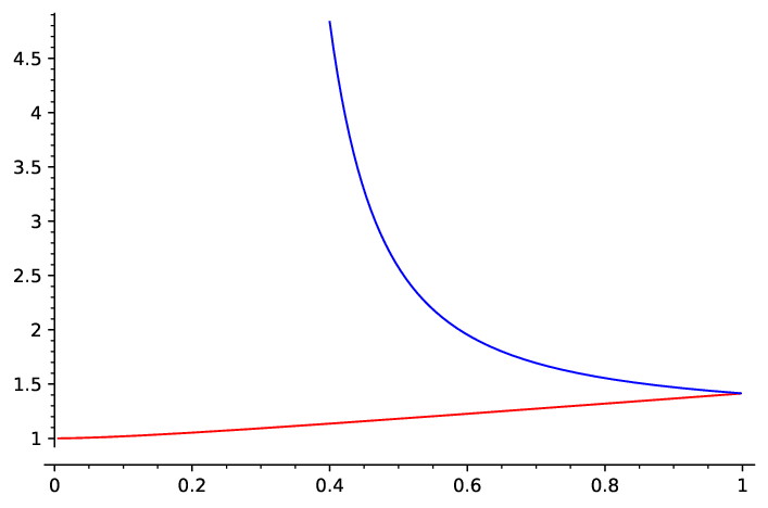
To introduce our second definition, it is important to observe that on ring-shaped model solutions the NWSS at either the inner or the outer boundary can be computed as a function of the core radius. More precisely, it is useful to consider the outer NWSS function $\overline{\tau}_{o}$ and the inner NWSS function $\overline{\tau}_{i}$, whose graphs are plotted in Figure 2 and which are defined as follows.

• •

  The outer NWSS function

  $$\overline{\tau}_{o}:[\,0,1)\longrightarrow[\,1,\sqrt{2}\,)$$

  (1.14)

  is defined by

  $$\hskip-42.67912pt\overline{\tau}_{o}(R)\,:=\,\frac{|\nabla u_{R}|}{\sqrt{2(u_{R})_{\rm max}}}\phantom{u\!\!}_{\big|_{\Gamma_{R,o}}}\!\!\!\!=\,\,\begin{cases}1,&\qquad\mbox{if }R=0,\\ \frac{1-R^{2}}{\sqrt{1-R^{2}+2R^{2}\log R}},&\qquad\mbox{if }0<R<1.\end{cases}$$

  (1.15)

  Observe that $\overline{\tau}_{o}$ is continuous, strictly increasing, and $\overline{\tau}_{o}(R)\to\sqrt{2}$, as $R\to 1^{-}$.

• •

  The inner NWSS function

  $$\overline{\tau}_{i}:(0,1\,]\longrightarrow[\,\sqrt{2},+\infty\,)$$

  (1.16)

  is defined by

  $$\,\,\,\overline{\tau}_{i}(R)\,:=\,\frac{|\nabla u_{R}|}{\sqrt{2(u_{R})_{\rm max}}}\phantom{u\!\!}_{\big|_{\Gamma_{R,i}}}\!\!\!\!\!\!=\,\,\begin{cases}\frac{R^{2}-r_{i}^{2}(R)}{r_{i}(R)\sqrt{1-R^{2}+2R^{2}\log R}},&\qquad\mbox{if }0<R<1,\\ \sqrt{2},&\qquad\mbox{if }R=1.\end{cases}$$

  (1.17)

  Observe that $\overline{\tau}_{i}$ is continuous, strictly decreasing, and $\overline{\tau}_{i}(R)\to+\infty$, as $R\to 0^{+}$.

As pointed out, the key feature of $\overline{\tau}_{o}$ and $\overline{\tau}_{i}$ is that they are invertible. Building on this property, we are now ready to introduce the notion of expected core radius. In analogy with the NWSS, this invariant can be associated to either a boundary component of $\partial\Omega$ or, more in general, to a connected component of $\Omega\setminus{\rm MAX}(u)$.

As it is immediate to check, the expected core radius of a boundary component of a ring-shaped model solution $(\Omega_{R},u_{R})$ coincides by construction with the value of its core radius parameter $R$. In other words we have

and the same is true for the expected core radius of either the outer or the inner region $R(\Omega_{R,o})=R=R(\Omega_{R,i})$. This picture also includes the extremal case of Serrin’s solution (1.2), where the expected core radius is actually equal to $0$.

It should be noticed that definition (1.18) differs from definition (1.20) in a subtle, though substantial way. In (1.18) the condition $1\leq\overline{\tau}(\Gamma)$ has to be imposed in order to get a number in the range of $\overline{\tau}_{o}$, that can be effectively used to define $R(\Gamma)$. Such a condition is not needed in (1.20), since it turns out to be always satisfied. In particular, the expected core radius $R(N)$ of a region $N\in\pi_{0}(\Omega\setminus{\rm MAX}(u))$ is always well defined, as such, it is obviously nonnegative and more remarkably it vanishes if and only if $(\Omega,u)$ is equivalent to Serrin’s solution (1.2). This fact is stated in the following theorem, where no assumption is made a priori on either the topology of $\Omega$, or the number its boundary components.

The above theorem can be regarded as a first instance of how effective the notion of expected core radius might be for classification purposes. A second instance is contained in the following theorem. It says in particular that if the expected core radius that is guessed at the outer boundary $R(\Gamma_{o})$ coincides with the one that is guessed at the inner boundary $R(\Gamma_{i})$, then the solution is rotationally symmetric and coincides up to scaling with $(\Omega_{R},u_{R})$, where $R(\Gamma_{o})=R=R(\Gamma_{i})$

It is important to observe that, in contrast with Theorem B, no constant Neumann data are imposed on $\partial\Omega$ in Theorem D. Concerning the condition $\overline{\tau}(\Gamma_{o})<\sqrt{2}$, it must be noticed that it is always satisfied on the model solutions, as ${\rm Im}(\overline{\tau}_{o})=[1,\sqrt{2})$. Building on this condition, we will deduce that

The first inequality implies that $R(\Gamma_{o})$ is well defined, whereas the second says that the NWSS at $\Gamma_{i}$ lies in the range of $\overline{\tau}_{i}$, as it is natural to expect in the model situation.

The results and techniques employed in this paper open the way to a number of natural questions and possibilities for further developments. In this subsection we select some of the ones that we consider more natural or stimulating.

Let us start with a basic, nonetheless fundamental, observation concerning our comparison algorithm. As it is clear from Subsection 1.3, in order to implement our method it is first crucial to select a rotationally symmetric solution to compare with. This is done by matching the NWSS of a region with the NWSS of the outer or inner region of a model solution. A common feature of all the rotationally symmetric solutions $(\Omega_{R},u_{R})$ is that the NWSS of the inner region $\Omega_{R,i}$ is greater than $\sqrt{2}$, whereas the NWSS of the outer region $\Omega_{R,o}$ is less than $\sqrt{2}$. It would be interesting to figure out whether this holds true for a general ring-shaped solution to (1.1), or whether there are counterexamples. In a broader sense, one would want to understand to what extent the fact that a region is outer or inner influences the NWSS of that region. In the following sections we will be able to answer this question in some special cases: for instance, we will show that, if the NWSS is constant on the boundary of our region, then the region has low NWSS if it is outer and high NWSS if it is inner, as expected (see Proposition 5.2). A complete answer to this question could potentially allow us to remove the hypothesis $\overline{\tau}(\Gamma_{o})<\sqrt{2}$ from Theorem D.

Another point that is worth commenting on is how the classical moving plane method compares with the method employed in this paper. As already mentioned in the discussion leading to Theorem 1.1, the moving plane method seems to be particularly effective in characterizing rotationally symmetric solutions that are monotonically decreasing along the radial coordinate. On the other hand, we will show that our comparison argument works well when dealing with monotonically increasing model solutions. It would then appear that the two methods are complementary. Indeed, the moving plane method will come to our aid when discussing the rigidity statement of Theorem B, as we will need to invoke Theorem 1.1 to deal with outer regions. It should however be stressed that, while the moving plane method has been extensively studied and its limitations are well understood (as well as its outstanding merits), our technique is essentially new, and the question is still open about whether and how far it is possible to extend its range of applicability. This point will be discussed in further details in the upcoming work [2], where it will be shown that our technique can be refined to deal with monotonically decreasing model solutions as well, albeit at some cost, such as more subtle arguments and slightly less general conclusions. It will be clear from [2] that the results in the present paper can all be proved relying solely on our comparison approach. Nevertheless, in this paper we preferred to exploit Theorem 1.1 in order to shorten and simplify the exposition.

Remaining on the topic of investigating the features of our technique, it would definitely be interesting to understand whether it can be employed to study other overdetermined problems. There are already some positive answers in this direction. For instance, similar comparison techniques have been used in [4, 5] to study static spacetimes with positive cosmological constant. Also, as it will be shown in an upcoming work, our strategy allows to study problem (1.1) in higher dimension as well. There are of course many other potential applications that deserve future investigation. For instance, a very natural direction would be the study of the problem $\Delta u=\delta_{o}$ inside a bounded domain containing the origin, since the rotationally symmetric solutions to this equation are very similar to the ones considered in this paper (namely, they are the same as (1.4) but with negative values of $R^{2}$). Another possible attempt would be to generalize the PDE considered in this paper, for instance considering the equation $\Delta u=f(u)$, for a suitable family of functions $f$.

It is also reasonable to expect that our comparison technique may find applications outside the realm of overdetermined boundary value problems. As a particularly relevant example, in [23] an estimate for the distance of the maximum points from the boundary is provided for solutions to (1.1). This is achieved through a comparison argument with Serrin’s solution (1.2) by means of a classical elliptic inequality (see the proof of [23, Lemma 2.2] for more details). One may wonder whether our comparison argument (more precisely the elliptic inequality and corresponding gradient estimate discussed in Subsection 3.2) can be exploited to prove similar results.

We conclude by mentioning a couple of other problems coming from physical models, that are somehow related to ours. Remaining in the realm of fluid-dynamics, similar symmetry results on annular domains have been recently discussed for the Euler equation in [17]. Another problem that is worth mentioning is the so called torsion problem, modeling the torsion of a bar with holes. From a mathematical viewpoint, this problem is very similar to the one discussed here, the only difference being the boundary condition in the inner boundary components. One of the main papers on this problem is the well known [25], where Schwarz symmetrization [27] is used to prove that the rotationally symmetric solutions to the torsion problem are characterized as the ones maximizing torsional rigidity. Among the recent progresses on this problem, we mention [24], based again on the moving plane method, and [11].

In the rest of the paper we will prove the results stated in this section. Section 2 is dedicated to the proof of Theorem C. This result is crucial as it grants us that Definition 2 is well posed, which in turn allows us to set up our comparison machinery. This is the topic of Section 3, where the important notion of pseudo-radial function is introduced and exploited to prove a sharp upper bound for the gradient of $u$. In Section 4 we will see that the gradient estimates lead to some curvature bounds for $\Gamma_{o}$, $\Gamma_{i}$, and ultimately to the proof of Theorem D. Such curvature bounds will also be used in Section 5, suitably coupled with the Pohozaev Identity, to obtain Theorem B. Finally, Section 6 is devoted to the proof of Theorem A.

This subsection is aimed at defining pseudo-radial functions, that is, a functions that mimic the behavior of the radial coordinate $|x|$ in the rotationally symmetric solutions (1.4). As above, let $N\in\pi_{0}(\Omega\setminus{\rm MAX}(u))$ and let $R=R(N)$ be its expected core radius. As in (1.4), we let $r_{i}=r_{i}(R)\in(0,R)$ be the smallest positive root of the function $\rho\mapsto 1-\rho^{2}+2R^{2}\log\rho$, and we define the function

A simple computation shows that $\partial F_{R}/\partial\psi=0$ if and only if $\psi=R$. As a consequence of the Implicit Function Theorem we have that there exist two smooth functions

such that $F_{R}(u,\psi_{-}(u))=0=F_{R}(u,\psi_{+}(u))$ for all $u\in[0,u_{{\rm max}}(m)]$. For future convenience, let us list some elementary properties of $\psi_{+}$ and $\psi_{-}$, that can be derived easily from their definition.

• •

  First of all, we can compute $\psi_{+}$, $\psi_{-}$ and their derivatives using the following formulæ

  $$u\,=\,\frac{1-\psi_{\pm}^{2}+2R^{2}\log\psi_{\pm}}{2}\,.$$

  (3.3)

  $$\dot{\psi}_{\pm}\,=\,-\frac{\psi_{\pm}}{\psi_{\pm}^{2}-R^{2}}\,,\qquad\ddot{\psi}_{\pm}\,=\,2\,\dot{\psi}_{\pm}^{3}+\frac{\dot{\psi}_{\pm}^{2}}{{\psi}_{\pm}}\,.$$

  (3.4)

• •

  The function $\psi_{-}$ takes values in $[r_{i}(R),R]$, hence $\psi_{-}^{2}\leq R^{2}$ and from (3.4) we deduce

  $$\dot{\psi}_{-}\,\geq\,0\,,\qquad\ddot{\psi}_{-}\,\geq\,0\,,\qquad\lim_{u\to(u_{R})_{\max}^{-}}\dot{\psi}_{-}\,=\,+\infty\,.$$

• •

  The function $\psi_{+}$ takes values in $[R,1]$, hence $\psi_{+}^{2}\geq R^{2}$ and from the first formula in (3.4) we deduce that $\dot{\psi}_{+}$ is nonpositive and diverges as $u$ approaches $(u_{R})_{\max}$. Moreover, the second formula in (3.4) can be rewritten as

  $$\ddot{\psi}_{+}\,=\,\dot{\psi}_{+}^{3}\left(1+R^{2}\psi_{+}^{-2}\right)\,,$$

  from which it follows $\ddot{\psi}_{+}\leq 0$. Summing up, we have

  $$\dot{\psi}_{+}\,\leq\,0\,,\qquad\ddot{\psi}_{+}\leq 0\,,\qquad\lim_{u\to(u_{R})_{\max}^{-}}\dot{\psi}_{+}\,=\,-\infty\,.$$

Coming back to our case of interest, we are now going to use the functions $\psi_{\pm}$ in order to define a pseudo-radial function on $N$. To this end, we distinguish the cases where the NWSS OF $N$ is either above or below the threshold value $\sqrt{2}$.

In analogy with (3.4) and for future convenience, we point out that the following relationships hold true between the derivatives of the pseudo-radial function $\Psi$ and the potential $u$.

From the definition of $\Psi$, given in (3.5), (3.6), we can also easily recover an explicit formula for the comparison function $W_{R}=|\nabla u_{R}|^{2}\circ\Psi$ as a function of the pseudo-radial function:

We are now ready to state the main result of this section, in which we prove that the function $W=|\nabla u|^{2}$ is bounded from above by $W_{R}=|\nabla u_{R}|^{2}\circ\Psi$, where $R=R(N)$ is the expected core radius of the region $N$, that we are considering.

References

- [1] B. Barrios, L. Montoro, and B. Sciunzi. On the moving plane method for nonlocal problems in bounded domains. Journal d’Analyse Mathématique, 135(1):37–57, 2018.
- [2] S. Borghini. Symmetry results for Serrin-type problems in doubly connected domains. In preparation.
- [3] S. Borghini, P. T. Chruściel, and L. Mazzieri. On the uniqueness of Schwarzschild-de Sitter spacetime. ArXiv Preprint Server https://arxiv.org/abs/1909.05941, 2019.
- [4] S. Borghini and L. Mazzieri. On the mass of static metrics with positive cosmological constant: I. Classical Quantum Gravity, 35(12):125001, 43, 2018.
- [5] S. Borghini and L. Mazzieri. On the mass of static metrics with positive cosmological constant: II. Comm. Math. Phys., 377(3):2079–2158, 2020.
- [6] B. Brandolini, C. Nitsch, P. Salani, and C. Trombetti. On the stability of the Serrin problem. Journal of Differential Equations, 245(6):1566–1583, 2008.
- [7] J. Busca and R. Manásevich. A Liouville-type theorem for Lane-Emden systems. Indiana University mathematics journal, pages 37–51, 2002.
- [8] G. Ciraolo, A. Figalli, and A. Roncoroni. Symmetry results for critical anisotropic p-laplacian equations in convex cones. Geometric and Functional Analysis, 30(3):770–803, 2020.
- [9] G. Ciraolo and L. Vezzoni. On Serrin’s overdetermined problem in space forms. manuscripta mathematica, 159(3):445–452, 2019.
- [10] M. G. Crandall and P. H. Rabinowitz. Bifurcation from simple eigenvalues. Journal of Functional Analysis, 8(2):321–340, 1971.
- [11] G. Crasta, I. Fragalà, and F. Gazzola. A sharp upper bound for the torsional rigidity of rods by means of web functions. Archive for rational mechanics and analysis, 164(3):189–211, 2002.
- [12] L. Damascelli, F. Pacella, and M. Ramaswamy. Symmetry of ground states of p-laplace equations via the moving plane method. Archive for rational mechanics and analysis, 148(4):291–308, 1999.
- [13] M. M. Fall and S. Jarohs. Overdetermined problems with fractional laplacian. ESAIM: Control, Optimisation and Calculus of Variations, 21(4):924–938, 2015.
- [14] I. Fragala and F. Gazzola. Partially overdetermined elliptic boundary value problems. Journal of Differential Equations, 245(5):1299–1322, 2008.
- [15] B. Gidas, W.-M. Ni, and L. Nirenberg. Symmetry and related properties via the maximum principle. Communications in Mathematical Physics, 68(3):209–243, 1979.
- [16] A. R. Gover and B. Ørsted. Universal principles for Kazdan-Warner and Pohozaev-Schoen type identities. Commun. Contemp. Math., 15(4):1350002, 27, 2013.
- [17] F. Hamel and N. Nadirashvili. Circular flows for the Euler equations in two-dimensional annular domains, and related free boundary problems. Journal of the European Mathematical Society, 2021.
- [18] N. Kamburov and L. Sciaraffia. Nontrivial solutions to Serrin’s problem in annular domains. In Annales de l’Institut Henri Poincaré C, Analyse non linéaire. Elsevier, 2020.
- [19] S. G. Krantz and H. R. Parks. A primer of real analytic functions. Birkhäuser Advanced Texts: Basler Lehrbücher. [Birkhäuser Advanced Texts: Basel Textbooks]. Birkhäuser Boston, Inc., Boston, MA, second edition, 2002.
- [20] S. Łojasiewicz. Une propriété topologique des sous-ensembles analytiques réels. In Les Équations aux Dérivées Partielles (Paris, 1962), pages 87–89. Éditions du Centre National de la Recherche Scientifique, Paris, 1963.
- [21] S. Łojasiewicz. Introduction to complex analytic geometry. Birkhäuser Verlag, Basel, 1991. Translated from the Polish by Maciej Klimek.
- [22] L. Ma and B. Liu. Symmetry results for decay solutions of elliptic systems in the whole space. Advances in Mathematics, 225(6):3052–3063, 2010.
- [23] R. Magnanini and G. Poggesi. The location of hot spots and other extremal points. arXiv preprint arXiv:2005.13175, 2020.
- [24] L. E. Payne and G. A. Philippin. On two free boundary problems in potential theory. Journal of mathematical analysis and applications, 161(2):332–342, 1991.
- [25] G. Pólya and A. Weinstein. On the torsional rigidity of multiply connected cross-sections. Annals of Mathematics, pages 154–163, 1950.
- [26] W. Reichel. Radial symmetry by moving planes for semilinear elliptic BVPs on annuli and other non-convex domains. In Elliptic and parabolic problems (Pont-à-Mousson, 1994), volume 325 of Pitman Res. Notes Math. Ser., pages 164–182. Longman Sci. Tech., Harlow, 1995.
- [27] H. A. Schwarz. Gesammelte mathematische abhandlungen, volume 260. American Mathematical Soc., 1972.
- [28] J. Serrin. A symmetry problem in potential theory. Archive for Rational Mechanics and Analysis, 43(4):304–318, 1971.
- [29] J. Serrin and H. Zou. Symmetry of ground states of quasilinear elliptic equations. Archive for rational mechanics and analysis, 148(4):265–290, 1999.
- [30] B. Sirakov. Symmetry for exterior elliptic problems and two conjectures in potential theory. Ann. Inst. H. Poincaré Anal. Non Linéaire, 18(2):135–156, 2001.
- [31] J. Souček and V. Souček. Morse-Sard theorem for real-analytic functions. Comment. Math. Univ. Carolinae, 13:45–51, 1972.
- [32] H. F. Weinberger. Remark on the preceding paper of Serrin. Arch. Rational Mech. Anal., 43:319–320, 1971.