跳到论文正文
W Papers独立论文阅读器 arXiv:2109.11096 论文正文 计算阅读时间 · 0%
引用这篇论文根据当前论文元数据生成,正式投稿前建议核对。


License: CC BY 4.0
arXiv:2109.11096v3 [math.AP] 27 Feb 2022

Existence of a weak solution to a nonlinear fluid-structure interaction problem with heat exchange

Václav Mácha    Boris Muha    Šárka Nečasová    Arnab Roy &\& Srđan Trifunović
Abstract

In this paper, we study a nonlinear interaction problem between a thermoelastic shell and a heat-conducting fluid. The shell is governed by linear thermoelasticity equations and encompasses a time-dependent domain which is filled with a fluid governed by the full Navier-Stokes-Fourier system. The fluid and the shell are fully coupled, giving rise to a novel nonlinear moving boundary fluid-structure interaction problem involving heat exchange. The existence of a weak solution is obtained by combining three approximation techniques – decoupling, penalization and domain extension. In particular, the penalization and the domain extension allow us to use the methods already developed for compressible fluids on moving domains. In such a way, the proof is more elegant and the analysis is drastically simplified. Let us stress that this is the first time the heat exchange in the context of fluid-structure interaction problems is considered.

1 Introduction

1.1 Motivation and literature review

The existence of global-in-time weak solutions to the equations related to fluid dynamics is one of the fundamental questions in the modern mathematical theory of fluid mechanics. In the case of the incompressible Navier-Stokes equations, the concept of a weak solution was introduced in seminal work of Leray [38], where also existence results are proved. The corresponding theory for a barotropic compressible fluids is significantly more complicated and was developed much later, starting by pioneering works by Lions [39] and Feireisl et. al. [16]. However, in many applications the assumption that the fluid is barotropic is too restrictive, e.g. [56, 61, 25]. Therefore, the mathematical theory of the full Navier-Stokes-Fourier system describing heat conducting fluid was developed quite recently, e.g. [43, 59, 11, 10, 15, 12, 17, 50].

On the other hand, the fluid interaction with elastic structures is common in many real life situations and understanding this interactions is of vital importance for applications, e.g. [2, 30]. We refer to such systems as fluid-structure interaction (FSI) systems. The mathematical analysis of FSI problems has been extensively studied in the last two decades and a lot of the progress has been achieved. However, most of the results concern the incompressible fluid case. The results on the existence of a weak solution typically deal with FSI problems where the elastic structure is described by a lower dimensional model of a plate/shell type, see [47, 8, 21, 37, 46, 57] and references within. Exceptions are works [1, 48] where the existence of a weak solution to FSI problems involving regularized, nonlinear, 3​D3D viscoelastic structure and linear multilayered structure, respectively, were proven. All these works consider large data case and a solution existing as long as geometry does not degenerate, i.e. self-contact does not occur. There are also lot of results on the local-in-time or small data existence of strong solutions to FSI problems, see e.g. [9, 28, 55, 40, 23] and references within. We conclude the literature review about FSI models with incompressible fluid with a recent paper [22], where global-in-time solution to a 2​D−1​D2D-1D FSI model with a viscoelastic beam was proven.

The mathematical literature dealing with FSI problems with compressible fluids is scarce. In [3, 32] the authors prove the existence of local-in-time regular solutions. Recently, local-in-time existence results for strong solutions have been established for the compressible fluid-damped beam interaction in a 2D/1D framework in [44] and for the compressible fluid-undamped wave interaction in a 3D/2D framework in [41]. The existence of a weak solution was proven in [5, 58] and in [4], a weak solution was obtained for an interaction problem between a compressible fluid and a 3D viscoelastic structure. To the best of our knowledge there are only a few very recent papers dealing with the mathematical analysis of FSI problems with a heat conducting fluid. In [42] the existence of a strong solution for small time or small data is proven in the case when there is an additional damping on the structure, while in [6] existence of a weak solution is obtained for an FSI problem with a nonlinear Koiter shell. In both of these papers the structure does not conduct heat.

1.2 Problem description

We consider the flow of heat conducting compressible fluid in a 3​D3D container with the heat conducting elastic boundary. The fluid domain is determined by elastic displacement which is in turn obtained by solving the linearized Koiter shell equation with the forcing coming from the fluid, i.e. the fluid and the structure are fully coupled and we consider a moving boundary problem.

1.2.1 The problem geometry

Let Ω⊂ℝ3\Omega\subset{\mathbb{R}}^{3} be an open, connected, bounded domain whose boundary ∂Ω\partial\Omega is parametrized by an injective mapping φ∈C3​(Γ,ℝ3)\varphi\in C^{3}(\Gamma;{\mathbb{R}}^{3}) such that ∂Ω=φ⁡(Γ)\partial\Omega=\varphi(\Gamma), where Γ=ℝ2/ℤ2\Gamma={\mathbb{R}}^{2}/{\mathbb{Z}}^{2} is the flat torus (or Γ=ℝ/ℤ\Gamma={\mathbb{R}}/{\mathbb{Z}} is a circle in 2D case). Ω\Omega represents the reference fluid configuration. We denote by 𝐧{\bf n} the unit outer normal to Ω\Omega. The assumption that Γ\Gamma is the flat torus is not very restrictive and is introduced for technical and presentational simplicity. It corresponds to the flow through a pipe with periodic boundary conditions which is common in applications. With slight abuse of notation we will identify functions defined on Γ\Gamma and ∂Ω\partial\Omega. We assume that the structure displacement is of the form w⁡(t,y)​𝐧​(y)w(t,y){\bf n}(y), y∈Γy\in\Gamma. The elastic boundary at time tt is given by the following mapping (see Figure 1):

Φw​(t,y)=φ⁡(y)+w⁡(t,y)​𝐧​(y)y∈Γ.\displaystyle\Phi_{w}(t,y)=\varphi(y)+w(t,y){\bf n}(y)\quad y\in\Gamma. (1.1)

By a classical result on the tubular neighborhood, e.g. [35, Section 10], there exist numbers a∂Ωa_{\partial\Omega}, b∂Ωb_{\partial\Omega} such that mapping Φw(t,.)\Phi_{w}(t,.) is injective for w⁡(t,y)∈(a∂Ω,b∂Ω)w(t,y)\in(a_{\partial\Omega},b_{\partial\Omega}). Therefore the middle line of the shell at time tt occupies the following region:

Γw​(t)\displaystyle\Gamma^{w}(t) :={Φw​(t,y):y∈Γ}.\displaystyle:=\{\Phi_{w}(t,y):y\in\Gamma\}.
Refer to caption
Figure 1: The fluid domain Ωw​(t)\Omega^{w}(t) determined by Γw​(t)\Gamma^{w}(t) - the shell at time tt. The figure represents a vertical section of the torus in 3D or the entire model in 2D.

The fluid domain at time tt, Ωw​(t)⊂ℝ3\Omega^{w}(t)\subset\mathbb{R}^{3}, is defined as the interior region of Γw​(t)\Gamma^{w}(t). More precisely, let Φ~w\tilde{\Phi}_{w} be an arbitrary injective smooth extension of Φw\Phi_{w} to Ω\Omega11 1 An extension is explicitly constructed in (5.10). Note that its explicit form is not necessary for the definition of the problem.. Then the fluid domain at time tt is defined by Ωw​(t):=Φ~w​(t,Ω).\Omega^{w}(t):=\tilde{\Phi}_{w}(t,\Omega). Note that the fluid domain is well defined if Φw(t,.)\Phi_{w}(t,.) is injective, which is true if condition w⁡(t,y)∈(a∂Ω,b∂Ω)w(t,y)\in(a_{\partial\Omega},b_{\partial\Omega}) is satisfied. Therefore, our existence result is valid as long as this conditions holds. This is a consequence of the physical nature of the problem. Namely, for large displacement ww, function Φw\Phi_{w} is not necessarily injective which introduces a domain degeneracy in the problem that corresponds to the self-contact of the shell. The question of how to analyse contact in the fluid-structure interaction is still largely open (see e.g. [26, 20, 19, 7, 27, 24, 60] and reference within) and is outside of the scope of this paper.

Remark 1.1.

Even though the assumption that the shell deforms only in 𝐧{\bf n} direction is somewhat restrictive from the physical point of view, it is nevertheless standard in the literature on weak solutions to FSI problems, e.g. [8, 37, 47, 46]. Namely, the existence of a weak solution to FSI problems with vector displacement is still out of reach with current state-of-the-art techniques and only available results in this direction use some kind of additional structure regularization, e.g. [49, 18].

Finally, we introduce some notation related to the geometry. Let ΓT=(0,T)×Γ\Gamma_{T}=(0,T)\times\Gamma be the shell space-time domain and

QTw=⋃t∈(0,T){t}×Ωw​(t),ΓTw=⋃t∈(0,T){t}×Γw​(t)Q_{T}^{w}=\bigcup_{t\in(0,T)}\{t\}\times\Omega^{w}(t),\;\Gamma^{w}_{T}=\bigcup_{t\in(0,T)}\{t\}\times\Gamma^{w}(t)

be the Eulerian fluid domain and the Eulerian elastic interface domain, respectively. Note that the fluid domain depends on ww which is an unknown of the considered FSI problem. The outer unit normal to the deformed configuration Ωw​(t)\Omega^{w}(t) is denoted by 𝐧w​(t){\bf n}^{w}(t) and is given by formula 𝐧w=∇Φ~w−τ𝐧|∇Φ~w−τ𝐧|\mathbf{n}^{w}=\frac{\nabla\tilde{\Phi}_{w}^{-\tau}\mathbf{n}}{|\nabla\tilde{\Phi}_{w}^{-\tau}\mathbf{n}|}. Finally, the surface element on the interface Γw​(t)\Gamma^{w}(t) is given by

dΓw(t)=SwdΓ,Sw:=det∇Φ~w|∇Φ~w−τ𝐧|.d\Gamma^{w}(t)=S^{w}d\Gamma,\quad S^{w}:=\text{det}\nabla\tilde{\Phi}_{w}|\nabla\tilde{\Phi}_{w}^{-\tau}\mathbf{n}|.

1.2.2 The shell

We use the following linear thermoelastic shell model to describe the dynamics of the elastic boundary [34, section 1.5]:

∂t2w+Δ2​w+Δ​θ−α1​Δ​∂tw−α2​∂t2Δ​w\displaystyle\partial_{t}^{2}w+\Delta^{2}w+\Delta\theta-\alpha_{1}\Delta\partial_{t}w-\alpha_{2}\partial_{t}^{2}\Delta w =\displaystyle= Sw​𝐅⋅𝐧,\displaystyle S^{w}{\mathbf{F}}\cdot\mathbf{n}, (1.2)
θt−Δ​θ−Δ​wt\displaystyle\theta_{t}-\Delta\theta-\Delta w_{t} =\displaystyle= Sw​q.\displaystyle S^{w}q. (1.3)

Here ww denotes the displacement of the shell central surface in the direction 𝐧{\bf n} with respect to the reference configuration Γ\Gamma and θ≥0\theta\geq 0 denotes the shell temperature. Here and in continuation of the paper we normalize all strictly positive physical positive constants since the proofs do not depend on their concrete values. α1\alpha_{1} and α2\alpha_{2} are coefficients of viscoelasticity and rotational inertia, respectively and we assume α1,α2≥0\alpha_{1},\alpha_{2}\geq 0. Moreover, 𝐅\mathbf{F} is surface force density acting on the shell. Since we consider a linear model for the thermoelastic shell, equation (1.3) is the entropy equation, and qq is the entropy flux.

1.2.3 The fluid

We consider the flow of the heat conducting compressible fluid which is described by the three dimensional Navier-Stokes-Fourier system (see e.g. [15]) defined on the moving domain QTwQ^{w}_{T}:

∂tρ+∇⋅(ρ​𝐮)\displaystyle\partial_{t}\rho+\nabla\cdot(\rho\mathbf{u}) =\displaystyle= 0,\displaystyle 0, (1.4)
∂t(ρ​𝐮)+∇⋅(ρ​𝐮⊗𝐮)+∇p\displaystyle\partial_{t}(\rho\mathbf{u})+\nabla\cdot(\rho\mathbf{u}\otimes\mathbf{u})+\nabla p =\displaystyle= ∇⋅𝕊,\displaystyle\nabla\cdot\mathbb{S}, (1.5)
∂t(ρ​s)+∇⋅(ρ​s​𝐮)+∇⋅(𝐪ϑ)\displaystyle\partial_{t}(\rho s)+\nabla\cdot(\rho s\mathbf{u})+\nabla\cdot\Big(\displaystyle{\frac{\mathbf{q}}{\vartheta}}\Big) =\displaystyle= σ.\displaystyle\sigma. (1.6)

The unknown of the fluid system are the fluid densisty ρ\rho, the fluid velocity 𝐮\mathbf{u} and the fluid temperature ϑ≥0\vartheta\geq 0. The equations (1.4), (1.5) and (1.6) represent mass conservation, balance of momentum and entropy balance, respectively. The pressure pp and the specific entropy ss are the thermodynamical variables and depends on the density ρ\rho and the temperature ϑ\vartheta. Moreover, σ\sigma is the entropy production rate and is given by formula:

σ=1ϑ​(𝕊:∇𝐮−𝐪ϑ⋅∇ϑ).\sigma=\frac{1}{\vartheta}\left(\mathbb{S}:\nabla\mathbf{u}-\frac{{\bf q}}{\vartheta}\cdot\nabla\vartheta\right). (1.7)

The viscous stress tensor is given by the Newton’s rheological law:

𝕊(ϑ,∇𝐮):=μ(ϑ)(∇𝐮+∇τ𝐮−23∇⋅𝐮)+ζ(ϑ)∇⋅𝐮,μ(ϑ)>0,ζ(ϑ)>0,\displaystyle\mathbb{S}(\vartheta,\nabla\mathbf{u}):=\mu(\vartheta)\big(\nabla\mathbf{u}+\nabla^{\tau}\mathbf{u}-\frac{2}{3}\nabla\cdot\mathbf{u}\big)+\zeta(\vartheta)\nabla\cdot\mathbf{u},\quad\mu(\vartheta)>0,\quad\zeta(\vartheta)>0,

and heat flux 𝐪\mathbf{q} by the Fourier’s law:

𝐪:=−κ(ϑ)∇ϑ,κ(ϑ)>0,\displaystyle\mathbf{q}:=-\kappa(\vartheta)\nabla\vartheta,\quad\kappa(\vartheta)>0,

where μ\mu, ζ\zeta are the viscosity coefficients and κ\kappa is the heat coefficient. Observe that, every smooth solution to (1.4)-(1.6) with (1.7) satisfy the following energy identity in (0,T)(0,T):

dd​t∫Ωw​(t)(12ρ|𝐮|2+ρe)+dd​t∫Γ(12|∂tw|2+12|Δw|2+α22|∇∂tw|2+12|θ|2)\displaystyle\displaystyle{\frac{d}{dt}\int_{\Omega^{w}(t)}\Big(\frac{1}{2}\rho|\mathbf{u}|^{2}+\rho e\Big)+\frac{d}{dt}\int_{\Gamma}\Big(\frac{1}{2}|\partial_{t}w|^{2}+\frac{1}{2}|\Delta w|^{2}+\frac{\alpha_{2}}{2}|\nabla\partial_{t}w|^{2}+\frac{1}{2}|\theta|^{2}\Big)}
=−∫Γ|∇θ|2−α1|∇∂tw|2.\displaystyle=-\displaystyle{\int_{\Gamma}|\nabla\theta|^{2}-\alpha_{1}|\nabla\partial_{t}w|^{2}}. (1.8)

1.2.4 The coupling conditions

Since we are considering a moving boundary problem we need to prescribe two sets of coupling conditions. The kinematic coupling conditions state that the velocity and the temperature are continuous on the interface ΓT\Gamma_{T}:

Continuity of the velocity: ∂tw​𝐧\displaystyle\partial_{t}w\mathbf{n} =𝐮∘Φw,\displaystyle=\quad\mathbf{u}\circ\Phi_{w}, (1.9)
Continuity of the temperature: θ\displaystyle\theta =ϑ∘Φw.\displaystyle=\quad\vartheta\circ\Phi_{w}. (1.10)

Dynamic coupling conditions describe the balance of forces and the balance of entropy on ΓT:\Gamma_{T}:

𝐅\displaystyle\mathbf{F} =−[(p−𝕊)𝐧w]∘Φw,\displaystyle=\quad-\big[\big(p-\mathbb{S}\big)\mathbf{n}^{w}\big]\circ\Phi_{w}, (1.11)
q\displaystyle q =−(𝐧w​𝐪​(ϑ)ϑ)∘Φw.\displaystyle=\quad-\Big(\frac{\mathbf{n}^{w}\mathbf{q}(\vartheta)}{\vartheta}\Big)\circ\Phi_{w}. (1.12)

1.2.5 The initial conditions

Finally, the initial data are prescribed:

ϑ⁡(0,⋅)=ϑ0​(⋅),ρ⁡(0,⋅)=ρ0,(ρ​𝐮)​(0,⋅)=(ρ​𝐮)0,\displaystyle\vartheta(0,\cdot)=\vartheta_{0}(\cdot),~\rho(0,\cdot)=\rho_{0},~(\rho\mathbf{u})(0,\cdot)=(\rho\mathbf{u})_{0}, (1.13)
w⁡(0,⋅)=w0,∂tw⁡(0,⋅)=v0,θ⁡(0,⋅)=θ0.\displaystyle w(0,\cdot)=w_{0},~\partial_{t}w(0,\cdot)=v_{0},~\theta(0,\cdot)=\theta_{0}. (1.14)

We assume that initial data satisfy the following regularity properties:

ρ0∈L53​(Ωw0),ρ0≥0,ρ0≢0,ρ0|ℝ3∖Ωw0=0,\displaystyle\rho_{0}\in L^{\frac{5}{3}}(\Omega^{w_{0}}),\quad\rho_{0}\geq 0,\quad\rho_{0}\not\equiv 0,\quad\rho_{0}|_{\mathbb{R}^{3}\setminus\Omega^{w_{0}}}=0, (1.15)
ρ0>0​ in ​{(X,z)∈Ωw0:(ρ​𝐮)0​(X,z)>0},(ρ​𝐮)02ρ0∈L1​(Ωw0),\displaystyle\rho_{0}>0\text{ in }\{(X,z)\in\Omega^{w_{0}}:(\rho\mathbf{u})_{0}(X,z)>0\},\quad\frac{(\rho\mathbf{u})_{0}^{2}}{\rho_{0}}\in L^{1}(\Omega^{w_{0}}), (1.16)
ϑ0>0a.e in ​Ωw0,(ρ​s)0=ρ0​s​(ϑ0,ρ0)∈L1​(Ωw0),\displaystyle\vartheta_{0}>0\quad\text{a.e in }\Omega^{w_{0}},\quad(\rho s)_{0}=\rho_{0}s(\vartheta_{0},\rho_{0})\in L^{1}(\Omega^{w_{0}}),\quad\quad\quad\quad (1.17)
v0∈L2​(Γ),α2​v0∈H1​(Γ),w0∈H2​(Γ),θ0∈L2​(Γ),θ0≥0,\displaystyle v_{0}\in L^{2}(\Gamma),\quad\sqrt{\alpha_{2}}v_{0}\in H^{1}(\Gamma),\ w_{0}\in H^{2}(\Gamma),\ \theta_{0}\in L^{2}(\Gamma),\quad\theta_{0}\geq 0, (1.18)
E0:=∫Ωw0(12​ρ0​|(ρ​𝐮)0|2+ρ0​e​(ϑ0,ρ0))+∫Γ(12​|v0|2+12​|Δ​w0|2+α22​|∇v0|2+12​|θ0|2)<∞,\displaystyle{E_{0}:=\displaystyle{\int_{\Omega^{w_{0}}}\Big(\frac{1}{2\rho_{0}}|(\rho\mathbf{u})_{0}|^{2}+\rho_{0}e(\vartheta_{0},\rho_{0})\Big)+\int_{\Gamma}\Big(\frac{1}{2}|v_{0}|^{2}+\frac{1}{2}|\Delta w_{0}|^{2}+\frac{\alpha_{2}}{2}|\nabla v_{0}|^{2}+\frac{1}{2}|\theta_{0}|^{2}\Big)}<\infty,}\quad\quad\quad\quad (1.19)

and the following compatibility condition:

a∂Ω<w0<b∂Ωon ​Γ.\displaystyle a_{\partial\Omega}<w_{0}<b_{\partial\Omega}\quad\text{on }\Gamma. (1.20)

1.3 Main result and significance

Before stating the main result, we need to introduce Constitutive relations of the quantities in (1.4)-(1.6) in terms of the independent state variables that characterize the material properties of the fluid. Here we use the quite general constitutive relations from [15, Section 1.4] which we briefly list for the convenience of the reader. We assume the viscosity coefficients μ\mu and ζ\zeta are continuously differentiable functions of the absolute temperature, namely μ,ζ∈C1[0,∞)\mu,\ \zeta\in C^{1}[0,\infty) and satisfy22 2 The strict positivity of ζ\zeta ensures that ‖∇𝐮+∇τ𝐮‖Lt,x2||\nabla\mathbf{u}+\nabla^{\tau}\mathbf{u}||_{L_{t,x}^{2}} can be controlled by the energy, which gives us the uniform bounds for 𝐮\mathbf{u} (see Lemma 3.70 and (3.72)).

0<μ¯​(1+ϑ)≤μ⁡(ϑ)≤μ¯​(1+ϑ),supϑ∈[0,∞)|μ′​(ϑ)|≤m¯,0<\underline{\mu}(1+\vartheta)\leq\mu(\vartheta)\leq\overline{\mu}(1+\vartheta),\quad\sup_{\vartheta\in[0,\infty)}|\mu^{\prime}(\vartheta)|\leq\overline{m}, (1.21)
0<ζ¯​(1+ϑ)≤ζ⁡(ϑ)≤ζ¯​(1+ϑ).0<\underline{\zeta}(1+\vartheta)\leq\zeta(\vartheta)\leq\overline{\zeta}(1+\vartheta). (1.22)

The heat coefficient κ\kappa can be decomposed into two parts

κ⁡(ϑ)=κM​(ϑ)+κR​(ϑ)\kappa(\vartheta)=\kappa_{M}(\vartheta)+\kappa_{R}(\vartheta) (1.23)

where κM,κR∈C1[0,∞)\kappa_{M},\ \kappa_{R}\in C^{1}[0,\infty) and

0<κR¯​(1+ϑ3)≤κR​(ϑ)≤κR¯​(1+ϑ3),0<\underline{\kappa_{R}}(1+\vartheta^{3})\leq\kappa_{R}(\vartheta)\leq\overline{\kappa_{R}}(1+\vartheta^{3}), (1.24)
0<κM¯​(1+ϑ)≤κM​(ϑ)≤κM¯​(1+ϑ).0<\underline{\kappa_{M}}(1+\vartheta)\leq\kappa_{M}(\vartheta)\leq\overline{\kappa_{M}}(1+\vartheta). (1.25)

In the above formulas μ¯\underline{\mu}, μ¯\overline{\mu}, m¯\overline{m}, η¯\overline{\eta}, κR¯\underline{\kappa_{R}}, κR¯\overline{\kappa_{R}}, κM¯\underline{\kappa_{M}}, κM¯\overline{\kappa_{M}} are positive constants.

The quantities pp, ee, and ss are continuously differentiable functions for positive values of ρ\rho, ϑ\vartheta and satisfy Gibbs’ equation

ϑ​D​s​(ρ,ϑ)=D​e​(ρ,ϑ)+p⁡(ρ,ϑ)​D​(1ρ)​ for all ​ρ,ϑ>0.\vartheta Ds(\rho,\vartheta)=De(\rho,\vartheta)+p(\rho,\vartheta)D\left(\frac{1}{\rho}\right)\mbox{ for all }\rho,\ \vartheta>0. (1.26)

Further, we assume the following state equation for the pressure and the internal energy

p⁡(ρ,ϑ)=pM​(ρ,ϑ)+pR​(ϑ),pR​(ϑ)=a3​ϑ4,a>0,p(\rho,\vartheta)=p_{M}(\rho,\vartheta)+p_{R}(\vartheta),\quad p_{R}(\vartheta)=\frac{a}{3}\vartheta^{4},\ a>0, (1.27)
e⁡(ρ,ϑ)=eM​(ρ,ϑ)+eR​(ρ,ϑ),ρ​eR​(ρ,ϑ)=a​ϑ4,e(\rho,\vartheta)=e_{M}(\rho,\vartheta)+e_{R}(\rho,\vartheta),\quad\rho e_{R}(\rho,\vartheta)=a\vartheta^{4}, (1.28)

and

s⁡(ρ,ϑ)=sM​(ρ,ϑ)+sR​(ρ,ϑ),ρ​sR​(ρ,ϑ)=43​a​ϑ3.s(\rho,\vartheta)=s_{M}(\rho,\vartheta)+s_{R}(\rho,\vartheta),\quad\rho s_{R}(\rho,\vartheta)=\frac{4}{3}a\vartheta^{3}. (1.29)

According to the hypothesis of thermodynamic stability the molecular components satisfy

∂pM∂ρ>0​ for all ​ρ,ϑ>0\frac{\partial p_{M}}{\partial\rho}>0\mbox{ for all }\rho,\ \vartheta>0 (1.30)

and

0<∂eM∂ϑ≤c​ for all ​ρ,ϑ>0.0<\frac{\partial e_{M}}{\partial\vartheta}\leq c\mbox{ for all }\rho,\ \vartheta>0. (1.31)

Moreover

limϑ→0+eM​(ρ,ϑ)=e¯M​(ρ)>0​ for any fixed ​ρ>0,\lim_{\vartheta\to 0^{+}}e_{M}(\rho,\vartheta)=\underline{e}_{M}(\rho)>0\mbox{ for any fixed }\rho>0, (1.32)

and

|ρ​∂eM​(ρ,ϑ)∂ρ|≤c​eM​(ρ,ϑ)​ for all ​ρ,ϑ>0.\left|\rho\frac{\partial e_{M}(\rho,\vartheta)}{\partial\rho}\right|\leq ce_{M}(\rho,\vartheta)\mbox{ for all }\rho,\ \vartheta>0. (1.33)

We suppose also that there is a function PP satisfying

P∈C1[0,∞),P(0)=0,P′(0)>0,P\in C^{1}[0,\infty),\ P(0)=0,\ P^{\prime}(0)>0, (1.34)

and two positive constants 0<Z¯<Z¯0<\underline{Z}<\overline{Z} such that

pM​(ρ,ϑ)=ϑ52​P​(ρϑ32)​ whenever ​0<ρ≤Z¯​ϑ32, or, ​ρ>Z¯​ϑ32p_{M}(\rho,\vartheta)=\vartheta^{\frac{5}{2}}P\left(\frac{\rho}{\vartheta^{\frac{3}{2}}}\right)\mbox{ whenever }0<\rho\leq\underline{Z}\vartheta^{\frac{3}{2}},\mbox{ or, }\rho>\overline{Z}\vartheta^{\frac{3}{2}} (1.35)

and

pM​(ρ,ϑ)=23​ρ​eM​(ρ,ϑ)​ for ​ρ>Z¯​ϑ32.p_{M}(\rho,\vartheta)=\frac{2}{3}\rho e_{M}(\rho,\vartheta)\mbox{ for }\rho>\overline{Z}\vartheta^{\frac{3}{2}}. (1.36)
Remark 1.2.

A prototype of the above pressure law reads

p⁡(ρ,ϑ)=c1​ρ53+c2​ρ​ϑ+a3​ϑ4,\displaystyle p(\rho,\vartheta)=c_{1}\rho^{\frac{5}{3}}+c_{2}\rho\vartheta+\frac{a}{3}\vartheta^{4},

with the corresponding internal energy and specific entropy of the form

e⁡(ρ,ϑ)=32​c1​ρ23+cv​ϑ+aρ​ϑ4,\displaystyle e(\rho,\vartheta)=\frac{3}{2}c_{1}\rho^{\frac{2}{3}}+c_{v}\vartheta+\frac{a}{\rho}\vartheta^{4},
s⁡(ρ,ϑ)=cv​ln⁡ϑ−c2​ln⁡ρ+4​a3​ρ​ϑ3,\displaystyle s(\rho,\vartheta)=c_{v}\ln\vartheta-c_{2}\ln\rho+\frac{4a}{3\rho}\vartheta^{3},

where a,c1,c2,cv>0a,c_{1},c_{2},c_{v}>0.

We will denote system (1.2)-(1.6), (1.9)-(1.14) together with the described constitutive relations (1.21)-(1.36) by FSI-HEAT. The main result of the paper is:

Theorem 1.1.

Let initial data (ρ0,(ρ​𝐮)0,ϑ0,(ρ​s)0,w0,v0,θ0)(\rho_{0},(\rho\mathbf{u})_{0},\vartheta_{0},(\rho s)_{0},w_{0},v_{0},\theta_{0}) satisfy assumptions (1.15)-(1.20) and α1+α2>0\alpha_{1}+\alpha_{2}>0. Moreover, assume that the hypotheses (1.21)-(1.36) are satisfied. Then there exists T>0T>0 and a weak solution to FSI-HEAT system in the sense of Definition 2.1 defined on (0,T)(0,T). Moreover, either T=+∞T=+\infty or the domain Ωw​(t)\Omega^{w}(t) degenerates as t→Tt\to T.

The main novelties of the present work are:

  1. 1.

    We consider a model where both the fluid and the structure conduct heat and there is heat coupling given through temperature continuity and entropy flux given in (1.10) and (1.12). While, in the context of fluid-structure interaction, heat-conducting fluids have been studied in [6] and thermoelastic structures have been studied in [58], to the best of our knowledge this is the first work that takes into account heat conduction of both components, and heat exchange between the components. One nice consequence of this approach is that we were able to prove that the plate temperature is positive which does not hold if one considers just a linear plate model without coupling it to the fluid with heat exchange.

  2. 2.

    The fluid model we consider is from [15], and the same result also holds for the model given in (1.37) below. This way, a wide range of physical cases are covered. In particular, we allow pressure laws which are not uniform and can change depending on the region of the (ρ,ϑ)(\rho,\vartheta)-plane (see (1.35) and (1.36)). This is very important in the case of gases, as they become fully ionized in the degenerate region ρ>ϑ32​Z¯\rho>\vartheta^{\frac{3}{2}}\overline{Z} and change their behavior.

  3. 3.

    From the methodological point of view, we introduced a new approach to construct the approximate solutions. More precisely, we introduced a construction scheme that combines three approximation methods - decoupling, penalization and domain extension. This allows to decouple the problem and directly use sophisticated results and methods that are already developed to study compressible fluid on the moving domains [31, 13, 14]. We emphasize that such approach significantly simplifies the proof and has potential for further generalization. Namely, since our approach is modular, it is robust and can be adapted to more general fluid and/or structure models.

Let us first point out, that due to stronger imbedding results, our result easily holds in the case when the fluid is 2D and the structure is 1D, even in the case α1=α2=0\alpha_{1}=\alpha_{2}=0:

Corollary 1.2.

The conclusion of Theorem 1.1 holds in 2D/1D case for α1+α2≥0\alpha_{1}+\alpha_{2}\geq 0.

Inclusion of rotational inertia or viscoelasticity is needed in our proof. However, we use this assumption only in certain parts of the proof related to the convergence properties of the approximate solutions, and do not use it in the construction. Therefore, if we consider somewhat less general constitutive assumptions, our result holds without adding an additional regularization to the plate equations (see Remark 3.2 for a detailed explanation).

Corollary 1.3.

Let us assume p⁡(ρ,ϑ)=ργ+ρ​ϑ+a3​ϑ4p(\rho,\vartheta)=\rho^{\gamma}+\rho\vartheta+\frac{a}{3}\vartheta^{4} and γ>127\gamma>\frac{12}{7} in 3D or γ>1\gamma>1 in 2D. Then conclusion of Theorem 1.1 holds also for α1=α2=0\alpha_{1}=\alpha_{2}=0.

Remark 1.3.

The above pressure form is a prototype of the following pressure law where pMp_{M} is given by

pM​(ρ,ϑ)=ϑγγ−1​P​(ρϑ1γ−1), whenever ​0<ρ≤Z¯​ϑ32, or, ​ρ>Z¯​ϑ32,p_{M}(\rho,\vartheta)=\vartheta^{\frac{\gamma}{\gamma-1}}P\left(\frac{\rho}{\vartheta^{\frac{1}{\gamma-1}}}\right),\mbox{ whenever }0<\rho\leq\underline{Z}\vartheta^{\frac{3}{2}},\mbox{ or, }\rho>\overline{Z}\vartheta^{\frac{3}{2}}, (1.37)
pM​(ρ,ϑ)=(γ−1)​ρ​eM​(ρ,ϑ)​ for ​ρ>Z¯​ϑ32.p_{M}(\rho,\vartheta)=(\gamma-1)\rho e_{M}(\rho,\vartheta)\mbox{ for }\rho>\overline{Z}\vartheta^{\frac{3}{2}}.

instead of (1.35)–(1.36). For more details about such model, see [51] for the 3​D3D case and [52] for the 2​D2D case.

Remark 1.4.

Even though our analysis is done for the 3​D3D fluid flow, we also included results for 2​D2D case (Corollaries 1.2, 1.3 and Remark 1.3). Namely, the analysis for the 2​D2D case is analogous for the following reasons. First, all the embedding results that we use are stronger in the 2​D2D case. Second, our proof relies on the theory for the Navier-Stokes-Fourier system which is analogous for 2​D2D case and the main difference in comparison to 3​D3D case is that one can prove results with milder restriction on exponent γ\gamma (see also recent result in 2​D2D case [53]).

Remark 1.5.

It seems that most thermoelastic plate models in literature (including our own) are based upon the assumptions that the temperature is small with respect to the reference temperature, and that the entropy depends linearly on temperature [34, Chapter 1.5]. While this makes sense for the stability analysis of plates, it is in contrast with the thermodynamical properties of our fluid, which has strictly positive and arbitrarly large temperature and has a component of the entropy which depends logarithmically on the temperature. A possible solution to this problem might be to derive a new nonlinear thermoelastic plate model specially for our interaction problem, under the assumption that the thermodynamical properties of the plate are similar to the ones of the fluid, and then study its interaction with a heat-conducting fluid. This is a topic for future research.

1.4 Outline of the proof and organization of the paper

The proof is split into three parts that correspond to various level of approximation in the construction of approximate solutions. Each step includes limiting procedure which uses standard tool for analysis of the compressible fluids equations.

  • Step 1

    Existence of a weak solution to the extended problem. In the first step we define the extended problem on a large domain BB. The extension involves approximation parameters η,ω,ν,λ\eta,\omega,\nu,\lambda and follows approach from [31, 13]. We also add pressure regularization with approximation parameter δ\delta. This regularization improves integrability of the pressure and by now standard in the analysis of compressible Navier-Stokes equations. In this step we prove existence of a weak solution to the extended problem (see Definition 3.1). In order to construct approximate solutions to the extended problem, we introduce time step parameter Δ​t\Delta t and a time marching scheme that combines a decoupling approach (of the fluid and the structure) with penalization of the kinematic coupling conditions. The discussion about ideas behind this approach is included at the end of Section 3.1. The main advantage of such approach is that the existence result for the fluid part [31] can be directly used.

  • Step 2

    Extension limit Here we study limit as extension parameters η,ω,ν,λ→0\eta,\omega,\nu,\lambda\to 0. In this part we adapt ides from [31] to pass to the limit and obtain a solution which is defined of the physical domain QTwQ^{w}_{T}.

  • Step 3

    Pressure regularization limit. The last step of the proof is standard and is common in all existence proofs of a weak solution to compressible fluid equations.

The paper is organized as follows. In the Section 2, we introduce a concept of weak solution. The next three sections correspond to the three steps of the proof as described above: Step 1 (Existence of a weak solution to the extended problem) is explained in Section 3, Step 2 (limit of extension parameters) and Step 3 (pressure regularization limit) are discussed in Section 4 and Section 5 respectively. Finally, we include two Appendices where some technical results are proved.

2 Weak solution

We will use a concept of a weak solution that corresponds to the concept used in [15, Chapter 2] for the Navier-Stokes-Fourier system. However, since we consider a coupled moving boundary problem, there are some significant differences which we briefly describe before introducing the formal definition. First, since the fluid domain is defined by the structure displacement, we work with function spaces defined on the non-cylindrical domains in time and space. Moreover, from the energy inequality we have w∈H2​(Γ)w\in H^{2}(\Gamma) which is below threshold of Lipschitz regularity that is needed for standard functional analytic results on Sobolev spaces, such as the trace Theorem and Korn’s inequality. This functional framework for FSI problems is by now standard, so we just refer to [8, Section 1.3] or [37, Section 2]. In particular, we will use the Lagrangian trace operator γ|Γw:C(Ωw)→C(Γ)\gamma_{|\Gamma^{w}}:C(\Omega^{w})\to C(\Gamma) is defined as

γ|Γwf:=f|Γw∘Φw.\displaystyle\gamma_{|\Gamma^{w}}f:=f_{|\Gamma^{w}}\circ\Phi_{w}.

and then extended to a continuous and bounded operator γ|Γw:W1,p(Ωw)→W1−1r,r(Γ)\gamma_{|\Gamma^{w}}:W^{1,p}(\Omega^{w})\to W^{1-\frac{1}{r},r}(\Gamma), for any 1<r<p1<r<p, [37, Corollary 2.9] (see also [45]). For time dependent functions and displacements, we will usually write

(γ|Γwf)(t,⋅)=γ|Γw(t)f(t,⋅).\displaystyle(\gamma_{|\Gamma^{w}}f)(t,\cdot)=\gamma_{|\Gamma^{w}(t)}f(t,\cdot).

Moreover, we prove the following version of Korn’s inequality (Lemma 3.9):

‖𝐮‖W1,p​(Ωw)2≤C⁡[‖∇𝐮+∇τ𝐮‖L2​(Ωw)2+∫Ωwρ​|𝐮|2],for any ​p<2,\displaystyle||\mathbf{u}||_{W^{1,p}(\Omega^{w})}^{2}\leq C\Big[||\nabla\mathbf{u}+\nabla^{\tau}\mathbf{u}||_{L^{2}(\Omega^{w})}^{2}+\int_{\Omega^{w}}\rho|\mathbf{u}|^{2}\Big],\quad\text{for any }p<2,

where constant CC blows up as pp goes to 22, and therefore we will use W1,pW^{1,p}, p<2p<2 space instead of H1H^{1} in the definition of weak solution. Finally, solution and test spaces depend on solution and are not linear spaces. The kinematic coupling conditions (1.9), (1.10) are incorporated into the solution spaces, while the dynamic coupling conditions (1.11) and (1.12) are implicitly prescribed via the weak formulation. Namely, 𝕊⁡(ϑ,∇𝐮),p⁡(ρ,ϑ)\mathbb{S}(\vartheta,\nabla\mathbf{u}),p(\rho,\vartheta) and 𝐪⁡(ϑ)ϑ\frac{\mathbf{q}(\vartheta)}{\vartheta} do not have well-defined traces on the interface, and therefore (1.11) and (1.12) are only formally satisfied in a weak formulation.

Definition 2.1.

(Weak solution) We say that (ϑ,ρ,𝐮,w,θ)(\vartheta,\rho,\mathbf{u},w,\theta) is a weak solution to the FSI-HEAT problem with initial data (ρ0,(ρ​𝐮)0,ϑ0,(ρ​s)0,w0,v0,θ0)(\rho_{0},(\rho\mathbf{u})_{0},\vartheta_{0},(\rho s)_{0},w_{0},v_{0},\theta_{0}) satisfying the assumptions (1.15)−(1.20)\eqref{initial1}-\eqref{ICComp}, if the following conditions hold:

  1. 1.

    ρ≥0\rho\geq 0, ρ∈L∞​(0,T,L53​(ℝ3))∩Ll​o​cq​([0,T]×Ωw​(t))\rho\in L^{\infty}(0,T;L^{\frac{5}{3}}(\mathbb{R}^{3}))\cap L_{loc}^{q}([0,T]\times\Omega^{w}(t)), for some33 3 Here, the additional integrability of density can only be obtained on compact subsets, rather than on the whole domain. This is because ww is not regular enough to ensure Lipschitz regularity of the fluid domain Ωw​(t)\Omega^{w}(t) (which also changes in time), so the standard improved estimates of the density based on the Bogovskii operator do not hold up to the boundary. q>53q>\frac{5}{3};
    𝐮∈L2​(0,T,W1,p​(Ωw​(t)))\mathbf{u}\in L^{2}(0,T;W^{1,p}(\Omega^{w}(t))) for any p<2p<2, ρ​|𝐮|2∈L∞​(0,T,L1​(ℝ3))\rho|\mathbf{u}|^{2}\in L^{\infty}(0,T;L^{1}(\mathbb{R}^{3}));
    ϑ>0\vartheta>0 a.e. in QTwQ_{T}^{w}, ϑ∈L∞​(0,T,L4​(Ωw​(t)))\vartheta\in L^{\infty}(0,T;L^{4}(\Omega^{w}(t)));
    ϑ,∇ϑ∈L2​(QTw)\vartheta,\nabla\vartheta\in L^{2}(Q_{T}^{w}), log⁡ϑ,∇log⁡ϑ∈L2​(QTw)\log\vartheta,\nabla\log\vartheta\in L^{2}(Q_{T}^{w});
    ρ​s,ρ​s​𝐮,qϑ∈L1​(QTw)\rho s,\rho s\mathbf{u},\frac{q}{\vartheta}\in L^{1}(Q_{T}^{w});
    w∈L∞​(0,T,H2​(Γ))∩W1,∞​(0,T,L2​(Γ))w\in L^{\infty}(0,T;H^{2}(\Gamma))\cap W^{1,\infty}(0,T;L^{2}(\Gamma)), α1​w∈H1​(0,T,H1​(Γ))\alpha_{1}w\in H^{1}(0,T;H^{1}(\Gamma)), α2​w∈W1,∞​(0,T,H1​(Γ))\alpha_{2}w\in W^{1,\infty}(0,T;H^{1}(\Gamma));
    θ>0\theta>0 a.e. on ΓT\Gamma_{T}, θ∈L∞​(0,T,L2​(Γ))∩L2​(0,T,H1​(Γ))\theta\in L^{\infty}(0,T;L^{2}(\Gamma))\cap L^{2}(0,T;H^{1}(\Gamma));
    ln⁡θ∈L2​(0,T,Hs​(Γ))\ln\theta\in L^{2}(0,T;H^{s}(\Gamma)), for any44 4 This comes from the fact that γ|Γwlnϑ=lnθ\gamma_{|\Gamma^{w}}\ln\vartheta=\ln\theta, see Lemma 3.10. s<12s<\frac{1}{2}.

  2. 2.

    The coupling conditions ∂tw𝐧=γ|Γw𝐮\partial_{t}w\mathbf{n}=\gamma_{|\Gamma^{w}}\mathbf{u} and ϑ=γ|Γwθ\vartheta=\gamma_{|\Gamma^{w}}\theta hold on ΓT\Gamma_{T}.

  3. 3.

    The renormalized continuity equation

    ∫QTwρ​B​(ρ)​(∂tφ+𝐮⋅∇φ)=∫QTwb⁡(ρ)​(∇⋅𝐮)​φ+∫Ωw0ρ0​B​(ρ0)​φ​(0,⋅),\displaystyle\int_{Q_{T}^{w}}\rho B(\rho)(\partial_{t}\varphi+\mathbf{u}\cdot\nabla\varphi)=\int_{Q_{T}^{w}}b(\rho)(\nabla\cdot\mathbf{u})\varphi+\int_{\Omega^{w_{0}}}\rho_{0}B(\rho_{0})\varphi(0,\cdot), (2.1)

    holds for all φ∈Cc∞​([0,T)×Ωw​(t)¯)\varphi\in C_{c}^{\infty}([0,T)\times\overline{\Omega^{w}(t)}) and any b∈L∞(0,∞)∩C[0,∞)b\in L^{\infty}(0,\infty)\cap C[0,\infty) such that b⁡(0)=0b(0)=0 with B⁡(ρ)=B⁡(1)+∫1ρb⁡(z)z2​𝑑zB(\rho)=B(1)+\int_{1}^{\rho}\frac{b(z)}{z^{2}}dz.

  4. 4.

    The coupled momentum equation

    ∫QTwρ​𝐮⋅∂t𝝋+∫QTw(ρ​𝐮⊗𝐮):∇𝝋+∫QTwp⁡(ρ,ϑ)​(∇⋅𝝋)−∫QTw𝕊⁡(ϑ,∇𝐮):∇𝝋\displaystyle\int_{Q_{T}^{w}}\rho\mathbf{u}\cdot\partial_{t}\boldsymbol{\varphi}+\int_{Q_{T}^{w}}(\rho\mathbf{u}\otimes\mathbf{u}):\nabla\boldsymbol{\varphi}+\int_{Q_{T}^{w}}p(\rho,\vartheta)(\nabla\cdot\boldsymbol{\varphi})-\int_{Q_{T}^{w}}\mathbb{S}(\vartheta,\nabla\mathbf{u}):\nabla\boldsymbol{\varphi}
    +∫ΓT∂tw∂tψ−∫ΓTΔwΔψ−α1∫ΓT∂t∇w⋅∇ψ+α2∫ΓT∂t∇w⋅∂t∇ψ+∫ΓT∇θ⋅∇ψ\displaystyle+\int_{\Gamma_{T}}\partial_{t}w\partial_{t}\psi-\int_{\Gamma_{T}}\Delta w\Delta\psi-\alpha_{1}\displaystyle\int_{\Gamma_{T}}\partial_{t}\nabla w\cdot\nabla\psi+\alpha_{2}\displaystyle\int_{\Gamma_{T}}\partial_{t}\nabla w\cdot\partial_{t}\nabla\psi+\int_{\Gamma_{T}}\nabla\theta\cdot\nabla\psi
    =−∫Ωw0(ρ𝐮)0⋅𝝋(0,⋅)−∫Γv0ψ(0,⋅)−α2∫Γ∇v0⋅∇ψ(0,⋅),\displaystyle=-\int_{\Omega^{w_{0}}}(\rho\mathbf{u})_{0}\cdot\boldsymbol{\varphi}(0,\cdot)-\int_{\Gamma}v_{0}\psi(0,\cdot)-\alpha_{2}\int_{\Gamma}\nabla v_{0}\cdot\nabla\psi(0,\cdot), (2.2)

    holds for all 𝝋∈Cc∞​([0,T)×Ωw​(t)¯)\boldsymbol{\varphi}\in C_{c}^{\infty}([0,T)\times\overline{\Omega^{w}(t)}) and ψ∈Cc∞​([0,T)×Γ)\psi\in C_{c}^{\infty}([0,T)\times\Gamma) such that γ|Γw𝝋=ψ𝐧\gamma_{|\Gamma^{w}}\boldsymbol{\varphi}=\psi\mathbf{n} on ΓT\Gamma_{T}.

  5. 5.

    The coupled entropy inequality

    ∫QTwρ​s​(∂tφ+𝐮⋅∇φ)−∫QTwκ(ϑ)∇ϑ⋅∇φϑ+∫QTwφϑ​(𝕊⁡(ϑ,∇𝐮):∇𝐮+κ⁡(ϑ)​|∇ϑ|2ϑ)\displaystyle\int_{Q_{T}^{w}}\rho s(\partial_{t}\varphi+\mathbf{u}\cdot\nabla\varphi)-\int_{Q_{T}^{w}}\frac{\kappa(\vartheta)\nabla\vartheta\cdot\nabla\varphi}{\vartheta}+\int_{Q_{T}^{w}}\frac{\varphi}{\vartheta}\Big(\mathbb{S}(\vartheta,\nabla\mathbf{u}):\nabla\mathbf{u}+\frac{\kappa(\vartheta)|\nabla\vartheta|^{2}}{\vartheta}\Big)
    +∫ΓTθ∂tψ~−∫ΓT∇θ⋅∇ψ~+∫ΓT∇w⋅∇∂tψ~\displaystyle+\int_{\Gamma_{T}}\theta\partial_{t}\tilde{\psi}-\int_{\Gamma_{T}}\nabla\theta\cdot\nabla\tilde{\psi}+\int_{\Gamma_{T}}\nabla w\cdot\nabla\partial_{t}\tilde{\psi}
    ≤−∫Ωw0ρ0s(ϑ0,ρ0)φ(0,⋅)−∫Γθ0ψ~(0,⋅)−∫Γ∇w0⋅∇ψ~(0,⋅)\displaystyle\leq-\int_{\Omega^{w_{0}}}\rho_{0}s(\vartheta_{0},\rho_{0})\varphi(0,\cdot)-\int_{\Gamma}\theta_{0}\tilde{\psi}(0,\cdot)-\int_{\Gamma}\nabla w_{0}\cdot\nabla\tilde{\psi}(0,\cdot) (2.3)

    holds for all non-negative φ∈Cc∞​([0,T)×Ωw​(t)¯)\varphi\in C_{c}^{\infty}([0,T)\times\overline{\Omega^{w}(t)}) and ψ~∈Cc∞​([0,T)×Γ)\tilde{\psi}\in C_{c}^{\infty}([0,T)\times\Gamma) such that γ|Γwφ=ψ~\gamma_{|\Gamma^{w}}\varphi=\tilde{\psi} on ΓT\Gamma_{T}.

  6. 6.

    The energy inequality

    ∫Ωw​(t)(12ρ|𝐮|2+ρe(ρ,ϑ))(t)+∫Γ(12|∂tw|2+12|Δw|2+α22|∇∂tw|2+12|θ|2)(t)\displaystyle\displaystyle{\int_{\Omega^{w}(t)}\Big(\frac{1}{2}\rho|\mathbf{u}|^{2}+\rho e(\rho,\vartheta)\Big)(t)+\int_{\Gamma}\Big(\frac{1}{2}|\partial_{t}w|^{2}+\frac{1}{2}|\Delta w|^{2}+\frac{\alpha_{2}}{2}|\nabla\partial_{t}w|^{2}+\frac{1}{2}|\theta|^{2}\Big)(t)}
    +∫0T∫Γα1|∇∂tw|2+|∇θ|2≤∫Ωw0(12​ρ0|(ρ𝐮)0|2+ρ0e(ϑ0,ρ0))\displaystyle+\displaystyle{\int_{0}^{T}\int_{\Gamma}\alpha_{1}|\nabla\partial_{t}w|^{2}}+|\nabla\theta|^{2}\leq\displaystyle{\int_{\Omega^{w_{0}}}\Big(\frac{1}{2\rho_{0}}|(\rho\mathbf{u})_{0}|^{2}+\rho_{0}e(\vartheta_{0},\rho_{0})\Big)}
    +∫Γ(12|v0|2+12|Δw0|2+α22|∇v0|2+12|θ0|2)\displaystyle+\int_{\Gamma}\Big(\frac{1}{2}|v_{0}|^{2}+\frac{1}{2}|\Delta w_{0}|^{2}+\frac{\alpha_{2}}{2}|\nabla v_{0}|^{2}+\frac{1}{2}|\theta_{0}|^{2}\Big) (2.4)

    holds for all t∈[0,T]t\in[0,T].

Remark 2.1.

(1) The derivation of coupled momentum equation for smooth solutions is standard and we refer to [5, 58] for more details. However, the coupled entropy inequality appears here for the first time and it is derived in Appendix B.
(2) In the above definition, we have both entropy and energy balances in the form of inequalities. While entropy balance being satisfied as an inequality is standard, the energy one is different from standard theory [15]. This is a consequence of the fact that we have additional dissipation terms on the interface due to the coupling with the thermoelastic shell, and weak solution is not regular enough to obtain compactness results needed to preserve the energy equality in the limiting procedure. Although this definition may seem restrictive, we argue that is sufficient. Namely, if we assume that a weak solution is regular enough, we can obtain that both entropy and energy inequalities hold as equalities. This is proved in Appendix B by following the ideas from [54].

Remark 2.2.

(Achieving the initial data). By the standard theory, one deduces from (2.1) that

ρ∈Cw​(0,T,L53​(ℝ3)),\displaystyle\rho\in C_{w}(0,T;L^{\frac{5}{3}}(\mathbb{R}^{3})),

and since (2.2) holds for any compactly supported function 𝛗∈Cc∞​(QTw)\boldsymbol{\varphi}\in C_{c}^{\infty}(Q_{T}^{w}) (with ψ=0\psi=0), one also has

ρ​𝐮∈Cw​(0,T,L54​(ℝ3)).\displaystyle\rho\mathbf{u}\in C_{w}(0,T;L^{\frac{5}{4}}(\mathbb{R}^{3})).

Consequently, the equation (2.2) implies

∫Γ∂tw(t,y)ψ(y)+α2∫Γ∇∂tw(t,y)⋅∇ψ(y)→∫Γv0ψ+α2∫Γ∇v0⋅∇ψ,as t→0,\displaystyle\int_{\Gamma}\partial_{t}w(t,y)\psi(y)+\alpha_{2}\int_{\Gamma}\nabla\partial_{t}w(t,y)\cdot\nabla\psi(y)\to\int_{\Gamma}v_{0}\psi+\alpha_{2}\int_{\Gamma}\nabla v_{0}\cdot\nabla\psi,\quad\text{as }t\to 0,

for any ψ∈C∞​(Γ)\psi\in C^{\infty}(\Gamma), which gives by density argument

limt→0[∫Γ∂twψ+α2∫Γ∇∂tw⋅∇ψ](t)=∫Γv0ψ+α2∫Γ∇v0⋅∇ψ,for any ψ∈L2(Γ), with α2ψ∈H1(Γ).\displaystyle\lim\limits_{t\to 0}\left[\int_{\Gamma}\partial_{t}w\psi+\alpha_{2}\int_{\Gamma}\nabla\partial_{t}w\cdot\nabla\psi\right](t)=\int_{\Gamma}v_{0}\psi+\alpha_{2}\int_{\Gamma}\nabla v_{0}\cdot\nabla\psi,\quad\text{for any }\psi\in L^{2}(\Gamma),\text{ with }\alpha_{2}\psi\in H^{1}(\Gamma).

However, since there is ψ∈H2​(Γ)\psi\in H^{2}(\Gamma) such that (ψ−α2​Δ​ψ)=ϕ(\psi-\alpha_{2}\Delta\psi)=\phi for every function ϕ∈L2​(Γ)\phi\in L^{2}(\Gamma), this implies

limt→0[∫Γ∂twψ+α2∫Γ∇∂tw⋅∇ψ](t)=limt→0[∫Γ∂twψ−∫Γ∂twα2Δψ](t)\displaystyle\lim\limits_{t\to 0}\left[\int_{\Gamma}\partial_{t}w\psi+\alpha_{2}\int_{\Gamma}\nabla\partial_{t}w\cdot\nabla\psi\right](t)=\lim\limits_{t\to 0}\left[\int_{\Gamma}\partial_{t}w\psi-\int_{\Gamma}\partial_{t}w\alpha_{2}\Delta\psi\right](t)
=limt→0[∫Γ∂tw⁡(ψ−α2​Δ​ψ)]​(t)=limt→0[∫Γ∂tw​ϕ]​(t)=∫Γv0​ϕ,for any ​ϕ∈L2​(Γ).\displaystyle=\lim\limits_{t\to 0}\left[\int_{\Gamma}\partial_{t}w\big(\psi-\alpha_{2}\Delta\psi\big)\right](t)=\lim\limits_{t\to 0}\left[\int_{\Gamma}\partial_{t}w\phi\right](t)=\int_{\Gamma}v_{0}\phi,\quad\text{for any }\phi\in L^{2}(\Gamma).

Therefore

limt→0[∫Γ∂tw​ψ]​(t)=∫Γv0​ψ,for any ​ψ∈L2​(Γ),\displaystyle\lim\limits_{t\to 0}\left[\int_{\Gamma}\partial_{t}w\psi\right](t)=\int_{\Gamma}v_{0}\psi,\quad\text{for any }\psi\in L^{2}(\Gamma),
limt→0[α2∫Γ∇∂tw⋅∇ψ](t)=α2∫Γ∇v0⋅∇ψ,for any ψ∈H1(Γ).\displaystyle\lim\limits_{t\to 0}\left[\alpha_{2}\int_{\Gamma}\nabla\partial_{t}w\cdot\nabla\psi\right](t)=\alpha_{2}\int_{\Gamma}\nabla v_{0}\cdot\nabla\psi,\quad\text{for any }\psi\in H^{1}(\Gamma).

Finally, the entropy inequality (2.3) yields

limt→0[∫Ωw(ρ​s​(ρ,ϑ))+∫Γθ]​(t)≥∫Ωw0ρ0​s​(ϑ0,ρ0)+∫Γθ0.\displaystyle\lim\limits_{t\to 0}\left[\int_{\Omega^{w}}\big(\rho s(\rho,\vartheta)\big)+\int_{\Gamma}\theta\right](t)\geq\int_{\Omega^{w_{0}}}\rho_{0}s(\vartheta_{0},\rho_{0})+\int_{\Gamma}\theta_{0}.

3 Step 1 - Extended problem

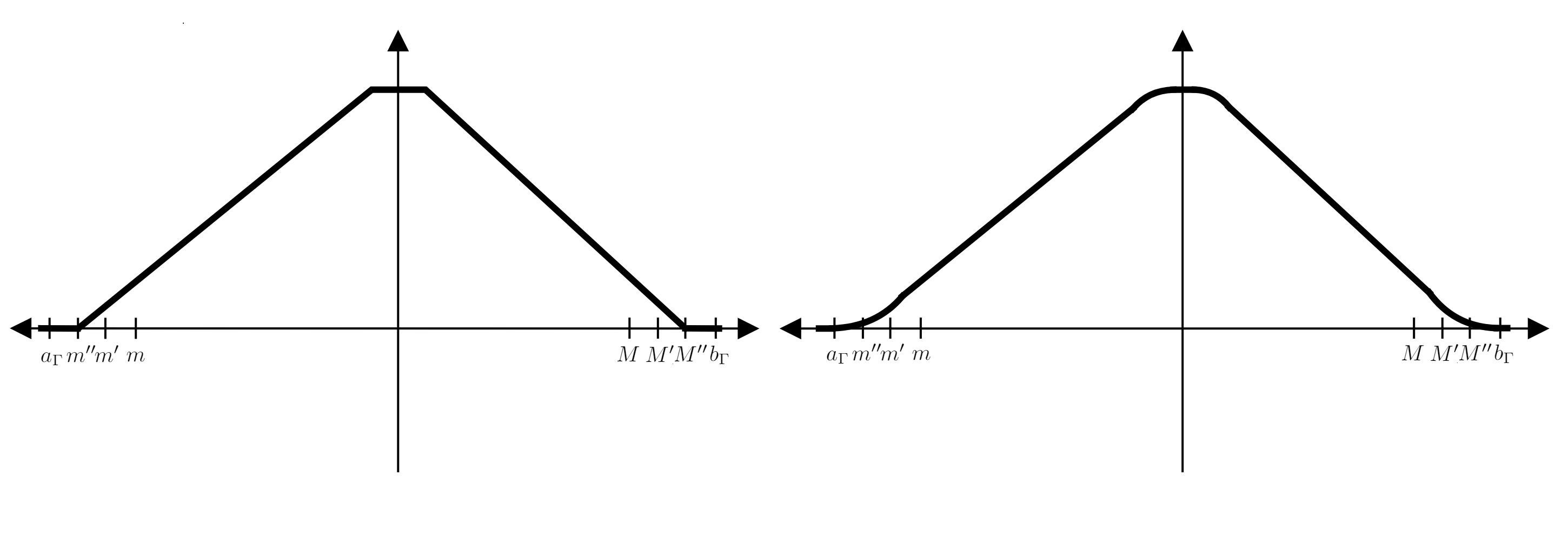
The first step in the construction of an approximate solution is to extend the problem to a large fixed domain which contains the physical domain Ωw​(t)\Omega^{w}(t) for every t∈[0,T]t\in[0,T]. Here we follow the approach from [31]. Let R>0R>0 be large enough so that Ωw(t)⊂B:={|X|<2R}\Omega^{w}(t)\subset B:=\{|X|<2R\} for all t∈[0,T]t\in[0,T]. Note that the displacement ww is bounded due to the energy estimates and thus such RR exists. Our constructed solution will satisfy the energy estimates, so this assumption is justified. The idea is to extend the problem onto BB (see figure 2) by extending the initial data, the viscosity coefficients and the heat conductivity coefficients in the following way.

Refer to caption
Figure 2: The fluid domain extended from Ωw​(t)\Omega^{w}(t) to BB.

3.1 Extension of data and coefficients

For a given ω>0\omega>0 and the structure displacement ww, the shear viscosity coefficients μ\mu and ζ\zeta (see (1.21)–(1.22)) are approximated as

μωw:=fωw​μ,ζωw:=fωw​ζ\displaystyle\mu_{\omega}^{w}:=f_{\omega}^{w}\mu,\quad\zeta_{\omega}^{w}:=f_{\omega}^{w}\zeta (3.1)

where fωwf_{\omega}^{w} Lipschitz continuously depends on ww and

fωw∈Cc∞([0,T]×ℝ3),0<ω≤fωw(t,x)≤1, in [0,T]×B,\displaystyle f_{\omega}^{w}\in C_{c}^{\infty}([0,T]\times\mathbb{R}^{3}),\quad 0<\omega\leq f_{\omega}^{w}(t,x)\leq 1,\text{ in }[0,T]\times B,
fωw(t,⋅)|Ωw(t)=1, for all t∈[0,T],||fωw||Lp​(((0,T)×B)∖QTw)≤Cωfor some p≥53.\displaystyle f_{\omega}^{w}(t,\cdot)_{|\Omega^{w}(t)}=1,\text{ for all }t\in[0,T],\quad||f_{\omega}^{w}||_{L^{p}(((0,T)\times B)\setminus Q_{T}^{w})}\leq C\omega\quad\text{for some }p\geq\frac{5}{3}.

Next, for a given ν>0\nu>0, the heat conductivity coefficient κ\kappa (see (1.23)−(1.25)\eqref{kappa_1}-\eqref{kappa_3}) is approximated by

κνw​(ϑ,t,x)=χνw​(t,x)​κ​(ϑ), where ​χνw=1​ in ​QTw​ and ​χνw=ν​ in ​((0,T)×B)∖QTw,\displaystyle\kappa_{\nu}^{w}(\vartheta,t,x)=\chi_{\nu}^{w}(t,x)\kappa(\vartheta),\text{ where }\chi_{\nu}^{w}=1\text{ in }Q_{T}^{w}\text{ and }\chi_{\nu}^{w}=\nu\text{ in }((0,T)\times B)\setminus Q_{T}^{w}, (3.2)

and similarly, the coefficient aa corresponding to the radiative part of the pressure, internal energy and energy (see (1.27)-(1.29)) is approximated by

aηw:=χηw​a, where ​χηw=1​ in ​QTw​ and ​χηw=η​ in ​((0,T)×B)∖QTw.\displaystyle a_{\eta}^{w}:=\chi_{\eta}^{w}a,\text{ where }\chi_{\eta}^{w}=1\text{ in }Q_{T}^{w}\text{ and }\chi_{\eta}^{w}=\eta\text{ in }((0,T)\times B)\setminus Q_{T}^{w}. (3.3)

The pressure is approximated as follows:

pη,δw:=pM​(ρ,ϑ)+aηw3​ϑ4+δ​ρβ,β≥4,δ>0,\displaystyle p_{\eta,\delta}^{w}:=p_{M}(\rho,\vartheta)+\frac{a_{\eta}^{w}}{3}\vartheta^{4}+\delta\rho^{\beta},\quad\beta\geq 4,\quad\delta>0, (3.4)

and the internal energy and specific entropy are approximated accordingly

eηw:=eM​(ρ,ϑ)+aηw​ϑ4ρ,sηw​(ρ,ϑ):=sM​(ρ,ϑ)+43​aηw​ϑ3ρ.\displaystyle e_{\eta}^{w}:=e_{M}(\rho,\vartheta)+a_{\eta}^{w}\frac{\vartheta^{4}}{\rho},\quad s_{\eta}^{w}(\rho,\vartheta):=s_{M}(\rho,\vartheta)+\frac{4}{3}a_{\eta}^{w}\frac{\vartheta^{3}}{\rho}. (3.5)

The initial data ρ0,(ρ​𝐮)0,ϑ0\rho_{0},(\rho\mathbf{u})_{0},\vartheta_{0} defined on Ωw0\Omega^{w_{0}} are extended and approximated by ρ0,δ,(ρ​𝐮)0,δ,ϑ0,δ\rho_{0,\delta},(\rho\mathbf{u})_{0,\delta},\vartheta_{0,\delta} as follows:

ρ0,δ≥0,ρ0,δ≢0,ρ0,δ|ℝ3∖Ωw0=0,∫B(ρ0,δ53+δ​ρ0,δβ)≤c,\displaystyle\rho_{0,\delta}\geq 0,~~\rho_{0,\delta}\not\equiv 0,~~\rho_{0,\delta}|_{\mathbb{R}^{3}\setminus\Omega^{w_{0}}}=0,~~\int_{B}\big(\rho_{0,\delta}^{\frac{5}{3}}+\delta\rho_{0,\delta}^{\beta}\big)\leq c, (3.6)
ρ0,δ→ρ0 in L53(B),|{ρ0,δ<ρ0}|→0, as δ→0,\displaystyle\rho_{0,\delta}\to\rho_{0}\text{ in }L^{\frac{5}{3}}(B),~~|\{\rho_{0,\delta}<\rho_{0}\}|\to 0,\text{ as }\delta\to 0, (3.7)
(ρ​𝐮)0,δ={(ρ​𝐮)0, if ​ρ0,δ≥ρ0,0, otherwise,∫B1ρ0,δ​|(ρ​𝐮)0,δ|2≤c,\displaystyle(\rho\mathbf{u})_{0,\delta}=\begin{cases}(\rho\mathbf{u})_{0},&\text{ if }\rho_{0,\delta}\geq\rho_{0},\\ 0,&\text{ otherwise}\end{cases},\quad\int_{B}\frac{1}{\rho_{0,\delta}}|(\rho\mathbf{u})_{0,\delta}|^{2}\leq c, (3.8)
ϑ0,δ≥ϑ¯≥0​ and ​ϑ0,δ∈L∞​(B)∩C2+ν​(B),\displaystyle\vartheta_{0,\delta}\geq\underline{\vartheta}\geq 0\text{ and }\vartheta_{0,\delta}\in L^{\infty}(B)\cap C^{2+\nu}(B), (3.9)

and ρ0,δ,ϑ0,δ\rho_{0,\delta},\vartheta_{0,\delta} are such that

∫Ωw0ρ0,δ​e​(ρ0,δ,ϑ0,δ)→∫Ωw0ρ0​e​(ρ0,ϑ0),ρ0,δ​s​(ρ0,δ,ϑ0,δ)⇀ρ0​s​(ρ0,ϑ0), in ​L1​(Ωw0),\displaystyle\begin{aligned} &\int_{\Omega^{w_{0}}}\rho_{0,\delta}e(\rho_{0,\delta},\vartheta_{0,\delta})\to\int_{\Omega^{w_{0}}}\rho_{0}e(\rho_{0},\vartheta_{0}),\\[5.69054pt] &\rho_{0,\delta}s(\rho_{0,\delta},\vartheta_{0,\delta})\rightharpoonup\rho_{0}s(\rho_{0},\vartheta_{0}),\text{ in }L^{1}(\Omega^{w_{0}}),\end{aligned} (3.10)

as δ→0\delta\to 0.

Now we define a weak solution to the extended FSI-HEAT problem on BB in the following way:

Definition 3.1.

(Weak solution to extended problem) We say that (ϑ,ρ,𝐮,w,θ)(\vartheta,\rho,\mathbf{u},w,\theta) is a weak solution to the extended FSI-HEAT problem if it satisfies the initial conditions (1.13), (1.14) and

  1. 1.

    ρ≥0\rho\geq 0, ρ∈L∞​(0,T,Lβ​(ℝ3))∩Ll​o​cq​([0,T]×(B¯∖Γw​(t)))\rho\in L^{\infty}(0,T;L^{\beta}(\mathbb{R}^{3}))\cap L_{loc}^{q}([0,T]\times(\overline{B}\setminus\Gamma^{w}(t))), for some q>53q>\frac{5}{3};
    Other regularity assumptions are the same as in Definition 2.1, but with the fluid quantities defined on (0,T)×B(0,T)\times B instead of QTwQ^{w}_{T}.

  2. 2.

    The coupling conditions ∂tw𝐧=γ|Γw𝐮\partial_{t}w\mathbf{n}=\gamma_{|\Gamma^{w}}\mathbf{u} and ϑ=γ|Γwθ\vartheta=\gamma_{|\Gamma^{w}}\theta hold on ΓT\Gamma_{T}.

  3. 3.

    The renormalized continuity equation

    ∫0T∫Bρ​B​(ρ)​(∂tφ+𝐮⋅∇φ)=∫0T∫Bb⁡(ρ)​(∇⋅𝐮)​φ+∫Bρ0,δ​B​(ρ0,δ)​φ​(0,⋅),\displaystyle\int_{0}^{T}\int_{B}\rho B(\rho)(\partial_{t}\varphi+\mathbf{u}\cdot\nabla\varphi)=\int_{0}^{T}\int_{B}b(\rho)(\nabla\cdot\mathbf{u})\varphi+\int_{B}\rho_{0,\delta}B(\rho_{0,\delta})\varphi(0,\cdot), (3.11)

    holds for all φ∈Cc∞​([0,T)×B)\varphi\in C_{c}^{\infty}([0,T)\times B) and any b∈L∞(0,∞)∩C[0,∞)b\in L^{\infty}(0,\infty)\cap C[0,\infty) such that b⁡(0)=0b(0)=0 with B⁡(ρ)=B⁡(1)+∫1ρb⁡(z)z2​𝑑zB(\rho)=B(1)+\int_{1}^{\rho}\frac{b(z)}{z^{2}}dz.

  4. 4.

    The coupled momentum equation of the form

    ∫0T∫Bρ​𝐮⋅∂t𝝋+∫0T∫B(ρ​𝐮⊗𝐮):∇𝝋+∫0T∫Bpη,δw​(ρ,ϑ)​(∇⋅𝝋)−∫0T∫B𝕊ωw​(ϑ,∇𝐮):∇𝝋\displaystyle\int_{0}^{T}\displaystyle\int_{B}\rho\mathbf{u}\cdot\partial_{t}\boldsymbol{\varphi}+\int_{0}^{T}\displaystyle\int_{B}(\rho\mathbf{u}\otimes\mathbf{u}):\nabla\boldsymbol{\varphi}+\int_{0}^{T}\displaystyle\int_{B}p_{\eta,\delta}^{w}(\rho,\vartheta)(\nabla\cdot\boldsymbol{\varphi})-\int_{0}^{T}\displaystyle\int_{B}\mathbb{S}_{\omega}^{w}(\vartheta,\nabla\mathbf{u}):\nabla\boldsymbol{\varphi}
    +∫ΓT∂tw∂tψ−∫ΓTΔwΔψ−α1∫ΓT∂t∇w⋅∇ψ+α2∫ΓT∂t∇w⋅∂t∇ψ+∫ΓT∇θ⋅∇ψ\displaystyle+\displaystyle\int_{\Gamma_{T}}\partial_{t}w\partial_{t}\psi-\displaystyle\int_{\Gamma_{T}}\Delta w\Delta\psi-\alpha_{1}\displaystyle\int_{\Gamma_{T}}\partial_{t}\nabla w\cdot\nabla\psi+\alpha_{2}\displaystyle\int_{\Gamma_{T}}\partial_{t}\nabla w\cdot\partial_{t}\nabla\psi+\displaystyle\int_{\Gamma_{T}}\nabla\theta\cdot\nabla\psi
    =−∫B(ρ𝐮)0⋅𝝋(0,⋅)−∫Γv0ψ(0,⋅)−α2∫Γ∇v0⋅∇ψ(0,⋅),\displaystyle=-\int_{B}(\rho\mathbf{u})_{0}\cdot\boldsymbol{\varphi}(0,\cdot)-\int_{\Gamma}v_{0}\psi(0,\cdot)-\alpha_{2}\int_{\Gamma}\nabla v_{0}\cdot\nabla\psi(0,\cdot), (3.12)

    holds for all 𝝋∈Cc∞​([0,T)×B)\boldsymbol{\varphi}\in C_{c}^{\infty}([0,T)\times B) and ψ∈C∞​([0,T)×Γ)\psi\in C^{\infty}([0,T)\times\Gamma) such that ψ𝐧=γ|Γw𝝋\psi\mathbf{n}=\gamma_{|\Gamma^{w}}\boldsymbol{\varphi} on ΓT\Gamma_{T}.

  5. 5.

    The coupled entropy balance of the form

    ∫0T∫Bρ​sηw​(∂tφ+𝐮⋅∇φ)−∫0T∫Bκνw(ϑ)∇ϑ⋅∇φϑ+⟨σω,νw;φ⟩[ℳ,C]​([0,T]×B¯)\displaystyle\int_{0}^{T}\int_{B}\rho s_{\eta}^{w}(\partial_{t}\varphi+\mathbf{u}\cdot\nabla\varphi)-\int_{0}^{T}\int_{B}\frac{\kappa_{\nu}^{w}(\vartheta)\nabla\vartheta\cdot\nabla\varphi}{\vartheta}+\langle\sigma_{\omega,\nu}^{w};\varphi\rangle_{[\mathcal{M},C]([0,T]\times\overline{B})}
    +λ∫0T∫Bϑ4φ+∫0T∫Γθ∂tψ~−∫0T∫Γ∇θ⋅∇ψ~+∫0T∫Γ∇w⋅∇∂tψ~\displaystyle+\lambda\int_{0}^{T}\int_{B}\vartheta^{4}\varphi+\int_{0}^{T}\int_{\Gamma}\theta\partial_{t}\tilde{\psi}-\int_{0}^{T}\int_{\Gamma}\nabla\theta\cdot\nabla\tilde{\psi}+\int_{0}^{T}\int_{\Gamma}\nabla w\cdot\nabla\partial_{t}\tilde{\psi}
    =−∫Bρsηw(ϑ0,δ,ρ0,δ)φ(0,⋅)−∫Γθ0ψ~(0,⋅)−∫Γ∇w0⋅∇ψ~(0,⋅)\displaystyle=-\int_{B}\rho s_{\eta}^{w}(\vartheta_{0,\delta},\rho_{0,\delta})\varphi(0,\cdot)-\int_{\Gamma}\theta_{0}\tilde{\psi}(0,\cdot)-\int_{\Gamma}\nabla w_{0}\cdot\nabla\tilde{\psi}(0,\cdot) (3.13)

    holds for all non-negative φ∈Cc∞​([0,T)×B)\varphi\in C_{c}^{\infty}([0,T)\times B) and ψ~∈Cc∞​([0,T)×Γ)\tilde{\psi}\in C_{c}^{\infty}([0,T)\times\Gamma) such that ψ~=γ|Γwφ\tilde{\psi}=\gamma_{|\Gamma^{w}}\varphi on ΓT\Gamma_{T}, where

    σω,νw≥1ϑ​(𝕊ωw​(ϑ,∇𝐮):∇𝐮+κνw​(ϑ)​|∇ϑ|2ϑ).\displaystyle\sigma_{\omega,\nu}^{w}\geq\frac{1}{\vartheta}\Big(\mathbb{S}_{\omega}^{w}(\vartheta,\nabla\mathbf{u}):\nabla\mathbf{u}+\frac{\kappa_{\nu}^{w}(\vartheta)|\nabla\vartheta|^{2}}{\vartheta}\Big).
  6. 6.

    The following energy inequality

    ∫B(12​ρ​|𝐮|2+ρ​eηw​(ρ,ϑ)+δβ−1​ρβ)​(t)+λ​∫0t∫Bϑ5+1−δ2​‖∂tw⁡(t)‖L2​(Γ)2+12​‖Δ​w​(t)‖L2​(Γ)2\displaystyle\displaystyle{\int_{B}\Big(\frac{1}{2}\rho|\mathbf{u}|^{2}+\rho e_{\eta}^{w}(\rho,\vartheta)+\frac{\delta}{\beta-1}\rho^{\beta}\Big)(t)}+\lambda\int_{0}^{t}\int_{B}\vartheta^{5}+\frac{1-\delta}{2}||\partial_{t}w(t)||_{L^{2}(\Gamma)}^{2}+\frac{1}{2}||\Delta w(t)||_{L^{2}(\Gamma)}^{2}
    +α22||∇∂tw(t)||L2​(Γ)2+1−δ2||θ(t)||L2​(Γ)2+∫0t∫Γ(α1|∇∂tw|2+|∇θ|2)\displaystyle\quad+\frac{\alpha_{2}}{2}||\nabla\partial_{t}w(t)||_{L^{2}(\Gamma)}^{2}+\frac{1-\delta}{2}||\theta(t)||_{L^{2}(\Gamma)}^{2}+\int_{0}^{t}\int_{\Gamma}\big(\alpha_{1}|\nabla\partial_{t}w|^{2}+|\nabla\theta|^{2}\big)
    ≤∫B(12​ρ0,δ​|(ρ​𝐮)0,δ|2+ρ0,δ​eηw​(ϑ0,δ,ρ0,δ)+δβ−1​ρ0,δβ)\displaystyle\leq\displaystyle{\int_{B}\Big(\frac{1}{2\rho_{0,\delta}}|(\rho\mathbf{u})_{0,\delta}|^{2}+\rho_{0,\delta}e_{\eta}^{w}(\vartheta_{0,\delta},\rho_{0,\delta})}+\frac{\delta}{\beta-1}\rho_{0,\delta}^{\beta}\Big)
    +12​‖v0,δ‖L2​(Γ)2+12​‖Δ​w0,δ‖L2​(Γ)2+α22​‖∇v0,δ‖2+12​‖θ0,δ‖L2​(Γ)2,\displaystyle\quad+\frac{1}{2}||v_{0,\delta}||_{L^{2}(\Gamma)}^{2}+\frac{1}{2}||\Delta w_{0,\delta}||_{L^{2}(\Gamma)}^{2}+\frac{\alpha_{2}}{2}||\nabla v_{0,\delta}||^{2}+\frac{1}{2}||\theta_{0,\delta}||_{L^{2}(\Gamma)}^{2}, (3.14)

    holds for all t∈(0,T]t\in(0,T].

Remark 3.1.

The solution defined in the above definition depends on the parameters ω,η,ν,λ,δ\omega,\eta,\nu,\lambda,\delta. However, in order to simplify the notation, we will not write this explicitly. Throughout the rest of the paper, we adapt the convention that we do write this explicit dependence on parameter only in the limiting procedure related to that parameter. When there is no possibility of confusion we will omit the parameters at all.

The advantage of this formulation is that the fluid equations are given on a time-independent domain BB and therefore, following ideas from [31], we can use the theory and the ideas developed for the Navier-Stokes-Fourier system. However, note the system in Definition 3.1 is still coupled and depends on the geometry through condition 2 and conditions on the test functions. Therefore, it is far from straightforward how to decouple the system and solve the fluid part separately. Here we use the decoupling method based on operator splitting from [58] (see also [47] where the splitting method in the context of FSI was introduced) which penalizes the fluid velocity and temperature to ensure the kinematic coupling conditions. More precisely, we split the time interval (0,T)(0,T) into subintervals of length Δ​t\Delta t. The approximate solution is constructed via time-marching procedure where in each time sub-interval we solve separately the fluid and the structure sub-problems (which are continuous in time). The decoupling is achieved thanks to the relaxation of the kinematic boundary conditions which are satisfied only approximately via penalization with parameter 1Δ​t\frac{1}{\Delta t}. Moreover, the sub-problems “communicate” with each other via the penalization terms. Physically, in the approximate problems we make the interface transparent so the fluid can pass through it (see figure 3). In the limit Δ​t→0\Delta t\to 0, the kinematic coupling conditions are satisfied and the interface Γw​(t)\Gamma^{w}(t) becomes impermeable, and therefore we obtain a weak solution to the extended problem from Definition 3.1.

Refer to caption
Figure 3: The penalized fluid problem on an extended domain BB. Here, the boundary Γw​(t)\Gamma^{w}(t) is dashed in order to emphasize that the fluid can pass through it.

3.2 Vanishing density outside of the physical domain Ωw\Omega^{w}

Before constructing a solution to the extended problem, we show that density vanishes outside of the physical domain:

Lemma 3.1.

Let ρ∈L∞​(0,T,L3​(B)),𝐮∈L2​(0,T,H01​(B))\rho\in L^{\infty}(0,T;L^{3}(B)),\mathbf{u}\in L^{2}(0,T;H_{0}^{1}(B)) satisfy the renormalized continuity equation (3.11) on (0,τ)(0,\tau) for any τ∈(0,T)\tau\in(0,T) and let w∈L∞​(0,T,H2​(Γ))∩W1,∞​(0,T,L2​(Γ))∩H1​(ΓT)w\in L^{\infty}(0,T;H^{2}(\Gamma))\cap W^{1,\infty}(0,T;L^{2}(\Gamma))\cap H^{1}(\Gamma_{T}). If

ρ(0,⋅)|B∖Ωw0≡0\displaystyle\rho(0,\cdot)_{|B\setminus\Omega^{w_{0}}}\equiv 0

then

ρ|B∖Ωw(t)(t,⋅)≡0,for a.a. t∈(0,T).\displaystyle\rho_{|B\setminus\Omega^{w}(t)}(t,\cdot)\equiv 0,\quad\text{for a.a. }t\in(0,T).
Proof.

The proof follows [13, Lemma 4.1], which is based on level set approach. Since our flow function is quite different and less regular to the one in the mentioned lemma, we provide a full proof.

Let g0∈C3​(B)g_{0}\in C^{3}(B) be such that

g0={0,on ​Γ∪∂B,>0,in ​B∖Ω,<0,elsewhere in ​ℝ3.\displaystyle g_{0}=\begin{cases}0,\quad&\text{on }\Gamma\cup\partial B,\\ >0,\quad&\text{in }B\setminus\Omega,\\ <0,\quad&\text{elsewhere in }\mathbb{R}^{3}.\end{cases}

and

∇g0​(X)=h⁡(d⁡(X))​𝐧​(π⁡(X)),h⁡(x)≥c>0\displaystyle\nabla g_{0}(X)=h(d(X))\mathbf{n}(\pi(X)),\quad h(x)\geq c>0 (3.15)

in a small neighbourhood of Γ\Gamma denoted by SΓS_{\Gamma}. Signed distance function dd and projection π\pi are defined by (5.9) and (5.8) in Appendix A. Denote

Φ:=Φ~wB,𝐕:=∂tΦ~wB∘(Φ~wB)−1.\displaystyle\Phi:=\tilde{\Phi}_{w}^{B},\quad\mathbf{V}:=\partial_{t}\tilde{\Phi}_{w}^{B}\circ(\tilde{\Phi}_{w}^{B})^{-1}.

where the flow function Φ~wB:[0,T]×B→B\tilde{\Phi}_{w}^{B}:[0,T]\times B\to B is defined precisely in (5.10). We introduce the function g:[0,T]×B→ℝg:[0,T]\times B\to\mathbb{R} defined as

g⁡(t,X):=g0​(Φ−1​(t,X))\displaystyle g(t,X):=g_{0}(\Phi^{-1}(t,X))

which is a solution to the following transport equation

∂tg+∇g⋅𝐕=0,g(0,⋅)=g0.\displaystyle\partial_{t}g+\nabla g\cdot\mathbf{V}=0,\quad g(0,\cdot)=g_{0}.

Before we proceed, let us calculate on [0,T]×Φ⁡(t,SΓ)[0,T]\times\Phi(t,S_{\Gamma})

∇g​(t,X)=∇(g0​(Φ−1​(t,X)))=∇g0​(Φ−1​(t,X))⋅∇Φ−1​(t,X)\displaystyle\nabla g(t,X)=\nabla\big(g_{0}(\Phi^{-1}(t,X))\big)=\nabla g_{0}\big(\Phi^{-1}(t,X)\big)\cdot\nabla\Phi^{-1}(t,X)
=∂𝐧⁡(π⁡(X))g0​(Φ−1​(t,X))​𝐧​(π⁡(X))⋅∇Φ−1​(t,X)=∂𝐧⁡(π⁡(X))g0​(Φ−1​(t,X))​∂𝐧⁡(π⁡(X))Φ−1​(t,X),\displaystyle=\partial_{\mathbf{n}(\pi(X))}g_{0}(\Phi^{-1}(t,X))\mathbf{n}(\pi(X))\cdot\nabla\Phi^{-1}(t,X)=\partial_{\mathbf{n}(\pi(X))}g_{0}(\Phi^{-1}(t,X))\partial_{\mathbf{n}(\pi(X))}\Phi^{-1}(t,X),

and since

∂𝐧⁡(π⁡(X))Φ−1​(t,X)=11+f′​(d⁡(X))​w​(t,π⁡(X))​𝐧​(π⁡(X)), in ​[0,T]×Φ⁡(t,SΓ),\displaystyle\partial_{\mathbf{n}(\pi(X))}\Phi^{-1}(t,X)=\frac{1}{1+f^{\prime}(d(X))w(t,\pi(X))}\mathbf{n}(\pi(X)),\quad\text{ in }[0,T]\times\Phi(t,S_{\Gamma}),

one obtains by (5.13), (5.14),(5.15)\eqref{jacobianphi1},\eqref{jacobianphi2} and (3.15)

∇g​(t,X)=h~​(t,X)​𝐧​(π⁡(X)),0<c≤h~​(t,X)≤C,for all ​(t,X)∈[0,T]×Φ⁡(t,SΓ).\displaystyle\nabla g(t,X)=\tilde{h}(t,X)\mathbf{n}(\pi(X)),\quad 0<c\leq\tilde{h}(t,X)\leq C,\quad\text{for all }(t,X)\in[0,T]\times\Phi(t,S_{\Gamma}). (3.16)


Next, fix ξ>0\xi>0 and let us test (3.11) by

φ=[min⁡{1ξ​g;1}]+,\displaystyle\varphi=\Big[\min\Big\{\frac{1}{\xi}g;1\Big\}\Big]^{+},

to obtain

∫B∖Ωw​(t)(ρφ)(τ)=1ξ∫0τ∫{0≤g(t,X)<ξ}(ρ∂tg+ρ𝐮⋅∇g).\displaystyle\int_{B\setminus\Omega^{w}(t)}(\rho\varphi)(\tau)=\frac{1}{\xi}\int_{0}^{\tau}\int_{\{0\leq g(t,X)<\xi\}}\Big(\rho\partial_{t}g+\rho\mathbf{u}\cdot\nabla g\Big). (3.17)

We can now calculate

ρ​∂tg+ρ​𝐮⋅∇g=ρ⁡(∂tg+𝐮⋅∇g)=ρ⁡(𝐕−𝐮)⋅∇g,\displaystyle\rho\partial_{t}g+\rho\mathbf{u}\cdot\nabla g=\rho\Big(\partial_{t}g+\mathbf{u}\cdot\nabla g\Big)=\rho(\mathbf{V}-\mathbf{u})\cdot\nabla g, (3.18)

where by (5.12), (3.15) and (3.16)

(𝐕−𝐮)⋅∇g∈L2​(0,T,W01,32​(B∖Ωw​(t))).\displaystyle(\mathbf{V}-\mathbf{u})\cdot\nabla g\in L^{2}(0,T;W_{0}^{1,\frac{3}{2}}(B\setminus\Omega^{w}(t))). (3.19)

Denoting

δ⁡(t,X):=dist​(X,Γw​(t)∪∂B),for ​(t,X)∈[0,τ]×(B∖Ωw​(t)),\displaystyle\delta(t,X):=\text{dist}(X,\Gamma^{w}(t)\cup\partial B),\quad\text{for }(t,X)\in[0,\tau]\times(B\setminus\Omega^{w}(t)),

(3.19) and Hardy’s inequality give us

1δ​(𝐕−𝐮)⋅∇g∈L2​(0,τ,L32​(B∖Ωw​(t))),\displaystyle\frac{1}{\delta}(\mathbf{V}-\mathbf{u})\cdot\nabla g\in L^{2}(0,\tau;L^{\frac{3}{2}}(B\setminus\Omega^{w}(t))), (3.20)

which by (3.18) and (3.17) imply

∫B∖Ωw​(t)(ρφ)(τ)=1ξ∫0τ∫{0≤g(t,X)<ξ}δρ​1δ​(𝐕−𝐮)⋅∇g⏟∈L2​(0,T,L1​(B)).\displaystyle\int_{B\setminus\Omega^{w}(t)}(\rho\varphi)(\tau)=\frac{1}{\xi}\int_{0}^{\tau}\int_{\{0\leq g(t,X)<\xi\}}\delta\underbrace{\rho\frac{1}{\delta}(\mathbf{V}-\mathbf{u})\cdot\nabla g}_{\in L^{2}(0,T;L^{1}(B))}.

Thus, taking into consideration

ℳ({0≤g(t,X)<ξ})→0,as ξ→0,\displaystyle\mathcal{M}(\{0\leq g(t,X)<\xi\})\to 0,\quad\text{as }\xi\to 0,

which follows from the uniform boundedness of Φ\Phi in C0,α​([0,T],C0,1−2​α​(B))C^{0,\alpha}([0,T];C^{0,1-2\alpha}(B)), 0<α<1/20<\alpha<1/2, the proof of this lemma will follow by passing to the limit ξ→0\xi\to 0 if we show

(t,X)∈[0,T]×(B∖Ωw​(t)),0≤g⁡(t,X)<ξ⟹δ⁡(t,X)ξ≤C.\displaystyle(t,X)\in[0,T]\times(B\setminus\Omega^{w}(t)),\quad 0\leq g(t,X)<\xi\implies\frac{\delta(t,X)}{\xi}\leq C.

We split the set B∖Ωw​(t)=S1​(t)∪S2​(t)B\setminus\Omega^{w}(t)=S_{1}(t)\cup S_{2}(t), where

S1​(t):={X∈B∖Ωw​(t):dist​(X,Γw​(t))>dist​(X,∂B)},\displaystyle S_{1}(t):=\{X\in B\setminus\Omega^{w}(t):\text{dist}(X,\Gamma^{w}(t))>\text{dist}(X,\partial B)\},
S2​(t):={X∈B∖Ωw​(t):dist​(X,Γw​(t))≤dist​(X,∂B)}\displaystyle S_{2}(t):=\{X\in B\setminus\Omega^{w}(t):\text{dist}(X,\Gamma^{w}(t))\leq\text{dist}(X,\partial B)\}

and fix a small enough ξ0>0\xi_{0}>0. First, it is easy to conclude that

(t,X)∈[0,T]×S2​(t),0≤g⁡(t,X)=g0​(X)<ξ≤ξ0⟹δ⁡(t,X)ξ≤C,\displaystyle(t,X)\in[0,T]\times S_{2}(t),\quad 0\leq g(t,X)=g_{0}(X)<\xi\leq\xi_{0}\implies\frac{\delta(t,X)}{\xi}\leq C,

by the regularity of g0g_{0} and ∂B\partial B, since Φ=i​d\Phi=id near ∂B\partial B. Next, since ξ0\xi_{0} was chosen to be small, one has

(t,X)∈[0,T]×S1​(t),0≤g⁡(t,X)=g0​(Φ−1​(t,X))<ξ≤ξ0⟹Φ−1​(t,X)∈SΓ.\displaystyle(t,X)\in[0,T]\times S_{1}(t),\quad 0\leq g(t,X)=g_{0}(\Phi^{-1}(t,X))<\xi\leq\xi_{0}\implies\Phi^{-1}(t,X)\in S_{\Gamma}.

so

δ⁡(t,X)≤|X−w⁡(t,π⁡(X))|\displaystyle\delta(t,X)\leq|X-w(t,\pi(X))|
≤1|min[0,T]×Φ(t.SΓ)∇g(t,X)⋅𝐧(π(X))|​(g⁡(t,X)−g⁡(w⁡(t,π⁡(X)))⏟=0)≤C​ξ,\displaystyle\leq\frac{1}{\Big|\min\limits_{[0,T]\times\Phi(t.S_{\Gamma})}\nabla g(t,X)\cdot\mathbf{n}(\pi(X))\Big|}(g(t,X)-\underbrace{g(w(t,\pi(X)))}_{=0})\leq C\xi,

from (3.16). Thus, we can pass to the limit ξ0≥ξ→0\xi_{0}\geq\xi\to 0, which concludes the proof. ∎

Corollary 3.2.

Under the assumptions of previous lemma, we have:

pM​(ρ,ϑ)=0,on ​(0,T)×(B∖Ωw​(t)).\displaystyle p_{M}(\rho,\vartheta)=0,\quad\text{on }(0,T)\times(B\setminus\Omega^{w}(t)).
Proof.

This directly follows from the previous lemma and the estimate (see [15, Page 54, Section 3.2])

0≤pM​(ρ,ϑ)≤c⁡(ρ53+ρ​ϑ).\displaystyle 0\leq p_{M}(\rho,\vartheta)\leq c(\rho^{\frac{5}{3}}+\rho\vartheta).

∎

3.3 The splitting

We split the time interval to N∈ℕN\in\mathbb{N} sub-intervals of length Δ​t=T/N\Delta t=T/N (the time derivatives are not discretized). We split the extended problem into two sub-problems, the fluid sub-problem (FSP) and the structure sub-problem (SSP). The splitting is done in the coupled momentum equation (3.12) and the coupled entropy inequality (3.13), and the kinematic coupling conditions (1.9) are not preserved after the splitting. More precisely, we introduce two auxiliary unknowns 𝐯\mathbf{v} and τ\tau representing the traces of the fluid velocity and the fluid temperature on the interface, respectively:

𝐯:=γ|Γw𝐮τ:=γ|Γwϑ.\displaystyle\mathbf{v}:=\gamma_{|\Gamma^{w}}\mathbf{u}\quad\tau:=\gamma_{|\Gamma^{w}}\vartheta.

Note that the kinematic coupling conditions are not satisfied on the level of approximate solutions, i.e. in general 𝐯≠∂tw​𝐧\mathbf{v}\neq\partial_{t}w\mathbf{n} and τ≠ϑ\tau\neq\vartheta. However, penalty terms will be included in the decoupled equations, which will ensure that kinematic coupling conditions are satisfied in the limit Δ​t→0.\Delta t\to 0. The fluid and the structure sub-problems are solved one at the time through a time-marching scheme as it is represented on the figure 4.

tt(X,z)(X,z)n​Δ​tn\Delta tOn [n​Δ​t,(n+1)​Δ​t]×Γ[n\Delta t,(n+1)\Delta t]\times\Gamma,for given (OPENρn,𝐮n,ϑn,wn,θn)\rho^{n},\mathbf{u}^{n},\vartheta^{n},{w}^{n},\theta^{n}) solve STRUCTURE (wn+1,θn+1)({w}^{n+1},\theta^{n+1})On [n​Δ​t,(n+1)​Δ​t]×B[n\Delta t,(n+1)\Delta t]\times B,for given (OPENwn+1,θn+1,ϑn,ρn,𝐮n){w}^{n+1},\theta^{n+1},\vartheta^{n},\rho^{n},\mathbf{u}^{n}) solve FLUID (ϑn+1,ρn+1,𝐮n+1)(\vartheta^{n+1},\rho^{n+1},\mathbf{u}^{n+1})
Figure 4: The diagram of the solving procedure. Here, the STRUCTURE and FLUID solvers corespond to (S​S​P)(SSP) and (F​S​P)(FSP) systems given in the next section.

For 1≤n≤N−11\leq n\leq N-1, the sub-problems consist of the following equations, corresponding to the equations of the weak formulation of the extended problem in the sense of Definition 3.1:

The structure sub-problem on [n​Δ​t,(n+1)​Δ​t]×Γ[n\Delta t,(n+1)\Delta t]\times\Gamma:

  1. 1.

    The structure part of the coupled momentum equation (3.12);

  2. 2.

    The structure part of the coupled entropy equation (3.13);

  3. 3.

    The structure part of the energy inequality. (6)

The fluid sub-problem on [n​Δ​t,(n+1)​Δ​t]×B[n\Delta t,(n+1)\Delta t]\times B:

  1. 1.

    The renormalized continuity equation (3.11);

  2. 2.

    The fluid part of the coupled momentum equation (3.12);

  3. 3.

    The fluid part of the entropy inequality (3.13);

  4. 4.

    The fluid part of the energy inequality (6).

We now go on to define the sub-problems precisely.

3.4 The sub-problems

Denote the translation in time by −Δ​t-\Delta t as

TΔ​t​f​(t):={f⁡(t−Δ​t),t∈[(n−1)Δt,nΔt],n≥1,f⁡(0),t∈[0,Δ​t].\displaystyle T_{\Delta t}f(t):=\begin{cases}f(t-\Delta t),&\quad t\in[(n-1)\Delta t,n\Delta t],n\geq 1,\\ f(0),&\quad t\in[0,\Delta t].\end{cases}


We now introduce the approximation scheme:

The structure sub-problem (SSP):
By induction on n≥0n\geq 0, assume that:

  • Case n=0n=0: w0​(0,⋅):=w0w^{0}(0,\cdot):=w_{0},  ∂tw0​(0,⋅):=v0\partial_{t}w^{0}(0,\cdot):=v_{0},  θ0​(0,⋅):=θ0\theta^{0}(0,\cdot):=\theta_{0} and

    𝐯0​(t,⋅):=v0​𝐧,τ0​(t,⋅):=θ0,for ​t∈[−Δ​t,0];\displaystyle\mathbf{v}^{0}(t,\cdot):=v_{0}\mathbf{n},\quad\tau^{0}(t,\cdot):=\theta_{0},\quad\text{for }t\in[-\Delta t,0];
  • Case n≥1n\geq 1: the solution (wn,θn)(w^{n},\theta^{n}) of (S​S​P)(SSP) and the solution (ϑn,ρn,𝐮n)(\vartheta^{n},\rho^{n},\mathbf{u}^{n}) of (F​S​P)(FSP) (defined below) are already obtained.

Find (wn+1,θn+1)(w^{n+1},\theta^{n+1}) so that:

  1. 1.

    wn+1∈W1,∞​(n​Δ​t,(n+1)​Δ​t,L2​(Γ))∩L∞​(n​Δ​t,(n+1)​Δ​t,H2​(Γ))w^{n+1}\in W^{1,\infty}(n\Delta t,(n+1)\Delta t;L^{2}(\Gamma))\cap L^{\infty}(n\Delta t,(n+1)\Delta t;H^{2}(\Gamma)),
    α1​wn+1∈H1​(n​Δ​t,(n+1)​Δ​t,H1​(Γ))\alpha_{1}w^{n+1}\in H^{1}(n\Delta t,(n+1)\Delta t;H^{1}(\Gamma)), α2​wn+1∈W1,∞​(n​Δ​t,(n+1)​Δ​t,H1​(Γ))\alpha_{2}w^{n+1}\in W^{1,\infty}(n\Delta t,(n+1)\Delta t;H^{1}(\Gamma)),
    θn+1∈L∞​(n​Δ​t,(n+1)​Δ​t,L2​(Γ))∩L2​(n​Δ​t,(n+1)​Δ​t,H1​(Γ))\theta^{n+1}\in L^{\infty}(n\Delta t,(n+1)\Delta t;L^{2}(\Gamma))\cap L^{2}(n\Delta t,(n+1)\Delta t;H^{1}(\Gamma)).

  2. 2.

    wn+1​(n​Δ​t,⋅)=wn​(n​Δ​t,⋅),∂twn+1​(n​Δ​t,⋅)=∂twn​(n​Δ​t,⋅)w^{n+1}(n\Delta t,\cdot)=w^{n}(n\Delta t,\cdot),~~\partial_{t}w^{n+1}(n\Delta t,\cdot)=\partial_{t}w^{n}(n\Delta t,\cdot) and θn+1​(n​Δ​t,⋅)=θn​(n​Δ​t,⋅)\theta^{n+1}(n\Delta t,\cdot)=\theta^{n}(n\Delta t,\cdot) in the weakly continuous sense in time.

  3. 3.

    The following structure heat equation

    (1−δ)​∫n​Δ​t(n+1)​Δ​t∫Γθn+1​∂tψ~−δ​∫n​Δ​t(n+1)​Δ​t∫Γθn+1−TΔ​t​τnΔ​t​ψ~\displaystyle(1-\delta)\displaystyle\int_{n\Delta t}^{(n+1)\Delta t}\displaystyle\int_{\Gamma}\theta^{n+1}\partial_{t}\tilde{\psi}-\delta\displaystyle\int_{n\Delta t}^{(n+1)\Delta t}\displaystyle\int_{\Gamma}\frac{\theta^{n+1}-T_{\Delta t}\tau^{n}}{\Delta t}\tilde{\psi}
    −∫n​Δ​t(n+1)​Δ​t∫Γ∇θn+1⋅∇ψ~−∫n​Δ​t(n+1)​Δ​t∫Γ∇∂twn+1⋅∇ψ~=∫n​Δ​t(n+1)​Δ​tdd​t∫Γθn+1ψ~\displaystyle\quad-\displaystyle\int_{n\Delta t}^{(n+1)\Delta t}\displaystyle\int_{\Gamma}\nabla\theta^{n+1}\cdot\nabla\tilde{\psi}-\displaystyle\int_{n\Delta t}^{(n+1)\Delta t}\displaystyle\int_{\Gamma}\nabla\partial_{t}w^{n+1}\cdot\nabla\tilde{\psi}=\displaystyle\int_{n\Delta t}^{(n+1)\Delta t}\frac{d}{dt}\int_{\Gamma}\theta^{n+1}\tilde{\psi}
    (3.21)

    holds for all ψ~∈C∞​([n​Δ​t,(n+1)​Δ​t]×Γ)\tilde{\psi}\in C^{\infty}([n\Delta t,(n+1)\Delta t]\times\Gamma).

  4. 4.

    The following plate equation

    (1−δ)​∫n​Δ​t(n+1)​Δ​t∫Γ∂twn+1​∂tψ−δ​∫n​Δ​t(n+1)​Δ​t∫Γ∂twn+1−TΔ​t​𝐯n⋅𝐧Δ​t​ψ\displaystyle(1-\delta)\displaystyle\int_{n\Delta t}^{(n+1)\Delta t}\displaystyle\int_{\Gamma}\partial_{t}w^{n+1}\partial_{t}\psi-\delta\displaystyle\int_{n\Delta t}^{(n+1)\Delta t}\displaystyle\int_{\Gamma}\frac{\displaystyle\partial_{t}w^{n+1}-T_{\Delta t}\mathbf{v}^{n}\cdot\mathbf{n}}{\displaystyle\Delta t}\psi
    −∫n​Δ​t(n+1)​Δ​t∫ΓΔwn+1Δψ−α1∫n​Δ​t(n+1)​Δ​t∫∇∂twn+1⋅∇ψ\displaystyle-\displaystyle\int_{n\Delta t}^{(n+1)\Delta t}\displaystyle\int_{\Gamma}\Delta w^{n+1}\Delta\psi-\alpha_{1}\displaystyle\int_{n\Delta t}^{(n+1)\Delta t}\int\nabla\partial_{t}w^{n+1}\cdot\nabla\psi
    +α2∫n​Δ​t(n+1)​Δ​t∫Γ∇∂twn+1⋅∂t∇ψ+∫n​Δ​t(n+1)​Δ​t∫Γ∇θn+1⋅∇ψ\displaystyle+\alpha_{2}\displaystyle\int_{n\Delta t}^{(n+1)\Delta t}\displaystyle\int_{\Gamma}\nabla\partial_{t}w^{n+1}\cdot\partial_{t}\nabla\psi+\displaystyle\int_{n\Delta t}^{(n+1)\Delta t}\displaystyle\int_{\Gamma}\nabla\theta^{n+1}\cdot\nabla\psi
    =(1−δ)​∫n​Δ​t(n+1)​Δ​tdd​t​∫Γ∂twn+1​ψ+α2​∫n​Δ​t(n+1)​Δ​tdd​t​∫Γ∂t∇wn+1⋅∇ψ\displaystyle=(1-\delta)\displaystyle\int_{n\Delta t}^{(n+1)\Delta t}\frac{d}{dt}\int_{\Gamma}\partial_{t}w^{n+1}\psi+\alpha_{2}\displaystyle\int_{n\Delta t}^{(n+1)\Delta t}\frac{d}{dt}\int_{\Gamma}\partial_{t}\nabla w^{n+1}\cdot\nabla\psi (3.22)

    holds for all ψ∈C∞​([n​Δ​t,(n+1)​Δ​t]×Γ){\psi}\in C^{\infty}([n\Delta t,(n+1)\Delta t]\times\Gamma).

  5. 5.

    The following energy inequality

    δ2​Δ​t​∫n​Δ​tt(‖∂twn+1−TΔ​t​𝐯n⋅𝐧‖L2​(Γ)2+‖∂twn+1‖L2​(Γ)2)+1−δ2​‖∂twn+1​(t)‖L2​(Γ)2\displaystyle\frac{\delta}{2\Delta t}\int_{n\Delta t}^{t}\big(||\partial_{t}w^{n+1}-T_{\Delta t}\mathbf{v}^{n}\cdot\mathbf{n}||_{L^{2}(\Gamma)}^{2}+||\partial_{t}w^{n+1}||_{L^{2}(\Gamma)}^{2}\big)+\frac{1-\delta}{2}||\partial_{t}w^{n+1}(t)||_{L^{2}(\Gamma)}^{2}
    +δ2​Δ​t∫n​Δ​tt(||θn+1−TΔ​tτn+1||L2​(Γ)2+||θn+1||L2​(Γ)2)+1−δ2||θn+1(t)||L2​(Γ)2\displaystyle\quad+\frac{\delta}{2\Delta t}\int_{n\Delta t}^{t}\big(||\theta^{n+1}-T_{\Delta t}\tau^{n+1}||_{L^{2}(\Gamma)}^{2}+||\theta^{n+1}||_{L^{2}(\Gamma)}^{2}\big)+\frac{1-\delta}{2}||\theta^{n+1}(t)||_{L^{2}(\Gamma)}^{2}
    +12||Δwn+1(t)||L2​(Γ)2+α22||∇∂twn+1(t)||L2​(Γ)2+∫n​Δ​tt∫Γ(α1|∇∂twn+1|2+|∇θn+1|2)\displaystyle\quad+\frac{1}{2}||\Delta w^{n+1}(t)||_{L^{2}(\Gamma)}^{2}+\frac{\alpha_{2}}{2}||\nabla\partial_{t}w^{n+1}(t)||_{L^{2}(\Gamma)}^{2}+\int_{n\Delta t}^{t}\int_{\Gamma}\big(\alpha_{1}|\nabla\partial_{t}w^{n+1}|^{2}+|\nabla\theta^{n+1}|^{2}\big)
    ≤1−δ2||∂twn+1(nΔt)||L2​(Γ)2+12||Δwn+1(nΔt)||L2​(Γ)2+α22||∇∂tw(nΔt)||L2​(Γ)2\displaystyle\leq\frac{1-\delta}{2}||\partial_{t}w^{n+1}(n\Delta t)||_{L^{2}(\Gamma)}^{2}+\frac{1}{2}||\Delta w^{n+1}(n\Delta t)||_{L^{2}(\Gamma)}^{2}+\frac{\alpha_{2}}{2}||\nabla\partial_{t}w(n\Delta t)||_{L^{2}(\Gamma)}^{2}
    +1−δ2​‖θn+1​(n​Δ​t)‖L2​(Γ)2+δ2​Δ​t​∫n​Δ​tt‖TΔ​t​𝐯n+1‖L2​(Γ)2+δ2​Δ​t​∫n​Δ​tt‖TΔ​t​τn+1‖L2​(Γ)2.\displaystyle\quad+\frac{1-\delta}{2}||\theta^{n+1}(n\Delta t)||_{L^{2}(\Gamma)}^{2}+\frac{\delta}{2\Delta t}\int_{n\Delta t}^{t}||T_{\Delta t}\mathbf{v}^{n+1}||_{L^{2}(\Gamma)}^{2}+\frac{\delta}{2\Delta t}\int_{n\Delta t}^{t}||T_{\Delta t}\tau^{n+1}||_{L^{2}(\Gamma)}^{2}.
    (3.23)

    holds for all t∈(n​Δ​t,(n+1)​Δ​t]t\in(n\Delta t,(n+1)\Delta t].

The fluid sub-problem (FSP):
By induction on n≥0n\geq 0, assume that:

  • Case n=0n=0: ρ0​(0,⋅):=ρ0,δ​(⋅)\rho^{0}(0,\cdot):=\rho_{0,\delta}(\cdot),  (ρ​𝐮)0​(0,⋅):=(ρ​𝐮)0,δ​(⋅)(\rho\mathbf{u})^{0}(0,\cdot):=(\rho\mathbf{u})_{0,\delta}(\cdot),  (ρ​s​(ρ,ϑ))0​(0,⋅):=(ρ0,δ​s​(ρ0,δ,ϑ0,δ))(\rho s(\rho,\vartheta))^{0}(0,\cdot):=(\rho_{0,\delta}s(\rho_{0,\delta},\vartheta_{0,\delta}));

  • Case n≥1n\geq 1: the solution (ϑn,ρn,𝐮n)(\vartheta^{n},\rho^{n},\mathbf{u}^{n}) of (F​S​P)(FSP) and the solution (wn+1,θn+1)(w^{n+1},\theta^{n+1}) of (S​S​P)(SSP) are already obtained.

Find (ϑn+1,ρn+1,𝐮n+1)(\vartheta^{n+1},\rho^{n+1},\mathbf{u}^{n+1}) so that:

  1. 1.

    ρn+1≥0\rho^{n+1}\geq 0, ρn+1∈L∞​(n​Δ​t,(n+1)​Δ​t,L53​(ℝ3))∩Ll​o​cq​([n​Δ​t,(n+1)​Δ​t],B¯∖Γw​(t)), for some ​q>53\rho^{n+1}\in L^{\infty}(n\Delta t,(n+1)\Delta t;L^{\frac{5}{3}}(\mathbb{R}^{3}))\cap L_{loc}^{q}([n\Delta t,(n+1)\Delta t];\overline{B}\setminus\Gamma^{w}(t)),\text{ for some }q>\frac{5}{3},
    ρn+1∈L∞​(n​Δ​t,(n+1)​Δ​t,Lβ​(ℝ3))\rho^{n+1}\in L^{\infty}(n\Delta t,(n+1)\Delta t;L^{\beta}(\mathbb{R}^{3})),
    𝐮n+1,∇𝐮n+1∈L2​((n​Δ​t,(n+1)​Δ​t)×B)\mathbf{u}^{n+1},\ \nabla\mathbf{u}^{n+1}\in L^{2}((n\Delta t,(n+1)\Delta t)\times B),   (ρ​𝐮)n+1∈L∞​(n​Δ​t,(n+1)​Δ​t,L1​(ℝ3))(\rho\mathbf{u})^{n+1}\in L^{\infty}(n\Delta t,(n+1)\Delta t;L^{1}(\mathbb{R}^{3})),
    ϑn+1>0\vartheta^{n+1}>0 a.e. in (n​Δ​t,(n+1)​Δ​t)×B(n\Delta t,(n+1)\Delta t)\times B,   ϑn+1∈L∞​(n​Δ​t,(n+1)​Δ​t,L4​(B))\vartheta^{n+1}\in L^{\infty}(n\Delta t,(n+1)\Delta t;L^{4}(B)),
    ϑn+1,∇ϑn+1∈L2​((n​Δ​t,(n+1)​Δ​t)×B)\vartheta^{n+1},\ \nabla\vartheta^{n+1}\in L^{2}((n\Delta t,(n+1)\Delta t)\times B),   log⁡ϑn+1,log⁡∇ϑn+1∈L2​((n​Δ​t,(n+1)​Δ​t)×B)\log\vartheta^{n+1},\ \log\nabla\vartheta^{n+1}\in L^{2}((n\Delta t,(n+1)\Delta t)\times B),
    (ρ​s)n+1,(ρ​s​𝐮)n+1,qn+1ϑn+1∈L1​((n​Δ​t,(n+1)​Δ​t)×B)(\rho s)^{n+1},(\rho s\mathbf{u})^{n+1},~~\frac{q^{n+1}}{\vartheta^{n+1}}\in L^{1}((n\Delta t,(n+1)\Delta t)\times B).

  2. 2.

    ρn+1​(n​Δ​t)=ρn​(n​Δ​t)\rho^{n+1}(n\Delta t)=\rho^{n}(n\Delta t), (ρ​𝐮)n+1​(n​Δ​t)=(ρ​𝐮)n​(n​Δ​t)(\rho\mathbf{u})^{n+1}(n\Delta t)=(\rho\mathbf{u})^{n}(n\Delta t) in weakly continuous sense in time.

  3. 3.

    The renormalized continuity equation

    ∫n​Δ​t(n+1)​Δ​t∫Bρn+1​B​(ρn+1)​(∂tφ+𝐮n+1⋅∇φ)\displaystyle\int_{n\Delta t}^{(n+1)\Delta t}\displaystyle\int_{B}\rho^{n+1}B(\rho^{n+1})(\partial_{t}\varphi+\mathbf{u}^{n+1}\cdot\nabla\varphi)
    =∫n​Δ​t(n+1)​Δ​t∫Bb⁡(ρn+1)​(∇⋅𝐮n+1)​φ−∫n​Δ​t(n+1)​Δ​tdd​t​∫Bρn+1​B​(ρn+1)​φ,\displaystyle=\int_{n\Delta t}^{(n+1)\Delta t}\displaystyle\int_{B}b(\rho^{n+1})(\nabla\cdot\mathbf{u}^{n+1})\varphi-\int_{n\Delta t}^{(n+1)\Delta t}\frac{d}{dt}\int_{B}\rho^{n+1}B(\rho^{n+1})\varphi,

    holds for all φ∈C∞​([n​Δ​t,(n+1)​Δ​t]×ℝ3)\varphi\in C^{\infty}([n\Delta t,(n+1)\Delta t]\times\mathbb{R}^{3}) and any b∈L∞(0,∞)∩C[0,∞)b\in L^{\infty}(0,\infty)\cap C[0,\infty) such that b⁡(0)=0b(0)=0 with B⁡(x)=B⁡(1)+∫1xb⁡(z)z2​𝑑zB(x)=B(1)+\int_{1}^{x}\frac{b(z)}{z^{2}}dz

  4. 4.

    The following momentum equation

    ∫n​Δ​t(n+1)​Δ​t∫Bρn+1​𝐮n+1⋅∂t𝝋+∫n​Δ​t(n+1)​Δ​t∫B(ρn+1​𝐮n+1⊗𝐮n+1):∇𝝋\displaystyle\int_{n\Delta t}^{(n+1)\Delta t}\displaystyle\int_{B}\rho^{n+1}\mathbf{u}^{n+1}\cdot\partial_{t}\boldsymbol{\varphi}+\int_{n\Delta t}^{(n+1)\Delta t}\displaystyle\int_{B}(\rho^{n+1}\mathbf{u}^{n+1}\otimes\mathbf{u}^{n+1}):\nabla\boldsymbol{\varphi}
    +∫n​Δ​t(n+1)​Δ​t∫Bpη,δn+1(ϑn+1,ρn+1)(∇⋅𝝋)−∫n​Δ​t(n+1)​Δ​t∫B𝕊ωn+1(ϑn+1,∇𝐮n+1):∇𝝋\displaystyle+\int_{n\Delta t}^{(n+1)\Delta t}\displaystyle\int_{B}p_{\eta,\delta}^{n+1}(\vartheta^{n+1},\rho^{n+1})(\nabla\cdot\boldsymbol{\varphi})-\int_{n\Delta t}^{(n+1)\Delta t}\displaystyle\int_{B}\mathbb{S}_{\omega}^{n+1}(\vartheta^{n+1},\nabla\mathbf{u}^{n+1}):\nabla\boldsymbol{\varphi}
    −δ∫n​Δ​t(n+1)​Δ​t∫Γ𝐯n+1−∂twn+1​𝐧Δ​t⋅𝝍=∫n​Δ​t(n+1)​Δ​tdd​t∫Bρn+1𝐮n+1⋅𝝋.\displaystyle-\delta\int_{n\Delta t}^{(n+1)\Delta t}\displaystyle\int_{\Gamma}\frac{\displaystyle\mathbf{v}^{n+1}-\partial_{t}w^{n+1}\mathbf{n}}{\displaystyle\Delta t}\cdot\boldsymbol{\psi}=\int_{n\Delta t}^{(n+1)\Delta t}\frac{d}{dt}\int_{B}\rho^{n+1}\mathbf{u}^{n+1}\cdot\boldsymbol{\varphi}. (3.24)

    holds for all 𝝋∈Cc∞​([n​Δ​t,(n+1)​Δ​t]×B)\boldsymbol{\varphi}\in C_{c}^{\infty}([n\Delta t,(n+1)\Delta t]\times B) and 𝝍∈C∞​(ΓT)\boldsymbol{\psi}\in C^{\infty}(\Gamma_{T}) such that γ|Γwn+1𝝋=𝝍\gamma_{|\Gamma^{w^{n+1}}}\boldsymbol{\varphi}=\boldsymbol{\psi} on ΓT\Gamma_{T}, where

    𝐯n+1=γ|Γwn+1𝐮n+1,\displaystyle\mathbf{v}^{n+1}=\gamma_{|\Gamma^{w^{n+1}}}\mathbf{u}^{n+1},
    𝕊ωn+1(ϑ,∇𝐮):=μωn+1(ϑ)(∇𝐮+∇τ𝐮−23∇⋅𝐮)+ζωn+1(ϑ)∇⋅𝐮,\displaystyle\mathbb{S}_{\omega}^{n+1}(\vartheta,\nabla\mathbf{u}):=\mu_{\omega}^{n+1}(\vartheta)\big(\nabla\mathbf{u}+\nabla^{\tau}\mathbf{u}-\frac{2}{3}\nabla\cdot\mathbf{u}\big)+\zeta_{\omega}^{n+1}(\vartheta)\nabla\cdot\mathbf{u},
    μωn+1:=μωwn+1,ζωn+1:=ζωwn+1,pη,δn+1:=pη,δwn+1,\displaystyle\mu_{\omega}^{n+1}:=\mu_{\omega}^{w^{n+1}},\quad\zeta_{\omega}^{n+1}:=\zeta_{\omega}^{w^{n+1}},\quad p_{\eta,\delta}^{n+1}:=p_{\eta,\delta}^{w^{n+1}},

    with, μωw\mu_{\omega}^{w}, ζωw\zeta_{\omega}^{w} and pη,δwp_{\eta,\delta}^{w} being defined in Section 3.

  5. 5.

    The following entropy balance

    ∫n​Δ​t(n+1)​Δ​t∫Bρn+1​sηn+1​(∂tφ+𝐮n+1⋅∇φ)−∫n​Δ​t(n+1)​Δ​t∫Bκνn+1(ϑn+1)∇ϑn+1⋅∇φϑn+1\displaystyle\int_{n\Delta t}^{(n+1)\Delta t}\int_{B}\rho^{n+1}s_{\eta}^{n+1}(\partial_{t}\varphi+\mathbf{u}^{n+1}\cdot\nabla\varphi)-\int_{n\Delta t}^{(n+1)\Delta t}\int_{B}\frac{\kappa_{\nu}^{n+1}(\vartheta^{n+1})\nabla\vartheta^{n+1}\cdot\nabla\varphi}{\vartheta^{n+1}}
    +⟨σω,νn+1;φ⟩[ℳ,C]​([n​Δ​t,(n+1)​Δ​t]×B¯)+λ​∫n​Δ​t(n+1)​Δ​t∫Bϑ4​φ\displaystyle+\langle\sigma_{\omega,\nu}^{n+1};\varphi\rangle_{[\mathcal{M},C]([n\Delta t,(n+1)\Delta t]\times\overline{B})}+\lambda\int_{n\Delta t}^{(n+1)\Delta t}\int_{B}\vartheta^{4}\varphi
    −δ∫n​Δ​tt∫Γτn+1−θn+1Δ​tψ~=(∫Bρn+1sηn+1φ)|n​Δ​t(n+1)​Δ​t\displaystyle-\delta\displaystyle\int_{n\Delta t}^{t}\int_{\Gamma}\frac{\tau^{n+1}-\theta^{n+1}}{\Delta t}\tilde{\psi}=\Big(\int_{B}\rho^{n+1}s_{\eta}^{n+1}\varphi\Big)\Big|_{n\Delta t}^{(n+1)\Delta t} (3.25)

    holds for any φ∈C∞​([n​Δ​t,(n+1)​Δ​t]×B)\varphi\in C^{\infty}([n\Delta t,(n+1)\Delta t]\times B) and ψ~∈C∞​([n​Δ​t,(n+1)​Δ​t]×Γ)\tilde{\psi}\in C^{\infty}([n\Delta t,(n+1)\Delta t]\times\Gamma) such that γ|Γwn+1φ=ψ\gamma_{|\Gamma^{w^{n+1}}}\varphi=\psi, where

    σω,νn+1≥1ϑn+1​(𝕊ω​(ϑn+1,∇𝐮n+1):∇𝐮n+1+κνn+1​(ϑn+1)​|∇ϑn+1|2ϑn+1)\displaystyle\sigma_{\omega,\nu}^{n+1}\geq\frac{1}{\vartheta^{n+1}}\Big(\mathbb{S}_{\omega}(\vartheta^{n+1},\nabla\mathbf{u}^{n+1}):\nabla\mathbf{u}^{n+1}+\frac{\kappa_{\nu}^{n+1}(\vartheta^{n+1})|\nabla\vartheta^{n+1}|^{2}}{\vartheta^{n+1}}\Big)

    and

    τn+1=γ|Γwn+1ϑn+1,sηn+1:=sηwn+1,κνn+1:=κνwn+1,\displaystyle\tau^{n+1}=\gamma_{|\Gamma^{w^{n+1}}}\vartheta^{n+1},\quad s_{\eta}^{n+1}:=s_{\eta}^{w^{n+1}},\quad\kappa_{\nu}^{n+1}:=\kappa_{\nu}^{w^{n+1}},

    with sηws_{\eta}^{w} and κνw\kappa_{\nu}^{w} being defined in Section 3.

  6. 6.

    The following energy inequality

    ∫B(12​ρn+1​|𝐮n+1|2+ρn+1​eηn+1​(ϑn+1,ρn+1)+δβ−1​(ρn+1)β)​(t)+λ​∫n​Δ​tt∫B(ϑn+1)5\displaystyle\displaystyle{\int_{B}\Big(\frac{1}{2}\rho^{n+1}|\mathbf{u}^{n+1}|^{2}+\rho^{n+1}e_{\eta}^{n+1}(\vartheta^{n+1},\rho^{n+1})+\frac{\delta}{\beta-1}(\rho^{n+1})^{\beta}\Big)(t)}+\displaystyle{\lambda\int_{n\Delta t}^{t}\int_{B}(\vartheta^{n+1})^{5}}
    +δ2​Δ​t∫n​Δ​tt∫Γ(|𝐯n+1−∂twn+1𝐧|2+|𝐯n+1|2)+δ2​Δ​t∫n​Δ​tt∫Γ(|τn+1−θn+1|2+|τn+1|2)\displaystyle+\displaystyle{\frac{\delta}{2\Delta t}\int_{n\Delta t}^{t}\int_{\Gamma}\Big(|\mathbf{v}^{n+1}-\partial_{t}w^{n+1}\mathbf{n}|^{2}+|\mathbf{v}^{n+1}|^{2}\Big)}+\displaystyle{\frac{\delta}{2\Delta t}\int_{n\Delta t}^{t}\int_{\Gamma}\Big(|\tau^{n+1}-\theta^{n+1}|^{2}+|\tau^{n+1}|^{2}\Big)}
    ≤∫B(12​ρn​|𝐮n|2+ρn​eηn​(ϑn,ρn))​(n​Δ​t)+δ2​Δ​t​∫n​Δ​tt∫Γ(|∂twn+1|2+|θn+1|2),\displaystyle\leq\displaystyle{\int_{B}\Big(\frac{1}{2}\rho^{n}|\mathbf{u}^{n}|^{2}+\rho^{n}e_{\eta}^{n}(\vartheta^{n},\rho^{n})\Big)(n\Delta t)}+\frac{\delta}{2\Delta t}\int_{n\Delta t}^{t}\int_{\Gamma}\Big(|\partial_{t}w^{n+1}|^{2}+|\theta^{n+1}|^{2}\Big), (3.26)

    holds for any t∈[n​Δ​t,(n+1)​Δ​t]t\in[n\Delta t,(n+1)\Delta t], where eηn+1:=eηwn+1e_{\eta}^{n+1}:=e_{\eta}^{w^{n+1}}, with eηwe_{\eta}^{w} being defined in Section 3.

  7. 7.

    The total dissipation inequality

    ∫B(12​ρn+1​|𝐮n+1|2+H1,ηn+1​(ρn+1,ϑn+1)−(ρn+1−ρ¯)​∂H1,ηn+1​(ρ¯,1)∂ρ−H1,ηn+1​(ρ¯,1)+δβ−1​(ρn+1)β)​(t)\displaystyle\displaystyle{\int_{B}\Big(\frac{1}{2}\rho^{n+1}|\mathbf{u}^{n+1}|^{2}+H_{1,\eta}^{n+1}(\rho^{n+1},\vartheta^{n+1})-(\rho^{n+1}-\overline{\rho})\frac{\partial H_{1,\eta}^{n+1}(\overline{\rho},1)}{\partial\rho}-H_{1,\eta}^{n+1}(\overline{\rho},1)+\frac{\delta}{\beta-1}(\rho^{n+1})^{\beta}\Big)(t)}
    +λ∫n​Δ​tt∫B(ϑn+1)5+∫n​Δ​tt∫B1ϑn+1(𝕊ωn+1(ϑn+1,∇𝐮n+1):∇𝐮n+1+κνn+1​(ϑn+1)​|∇ϑn+1|2ϑn+1)\displaystyle+\lambda\int_{n\Delta t}^{t}\int_{B}(\vartheta^{n+1})^{5}+\int_{n\Delta t}^{t}\int_{B}\frac{1}{\vartheta^{n+1}}\Big(\mathbb{S}_{\omega}^{n+1}(\vartheta^{n+1},\nabla\mathbf{u}^{n+1}):\nabla\mathbf{u}^{n+1}+\frac{\kappa_{\nu}^{n+1}(\vartheta^{n+1})|\nabla\vartheta^{n+1}|^{2}}{\vartheta^{n+1}}\Big)
    +δ2​Δ​t∫n​Δ​tt∫Γ(|𝐯n+1−∂twn+1𝐧|2+|vn+1|2)+δ2​Δ​t∫n​Δ​tt∫Γ(|τn+1−θn+1|2+|τn+1|2)\displaystyle+\frac{\delta}{2\Delta t}\int_{n\Delta t}^{t}\int_{\Gamma}\Big(|\mathbf{v}^{n+1}-\partial_{t}w^{n+1}\mathbf{n}|^{2}+|v^{n+1}|^{2}\Big)+\displaystyle{\frac{\delta}{2\Delta t}\int_{n\Delta t}^{t}\int_{\Gamma}\Big(|\tau^{n+1}-\theta^{n+1}|^{2}+|\tau^{n+1}|^{2}\Big)}
    ≤∫B(12​ρn​|𝐮n|2+H1,ηn​(ρn,ϑn)−(ρn−ρ¯)​∂H1,ηn​(ρ¯,1)∂ρ−H1,ηn​(ρ¯,1)+ρn​e​(ϑn,ρn))​(n​Δ​t)\displaystyle\leq\displaystyle{\int_{B}\Big(\frac{1}{2}\rho^{n}|\mathbf{u}^{n}|^{2}+H_{1,\eta}^{n}(\rho^{n},\vartheta^{n})-(\rho^{n}-\overline{\rho})\frac{\partial H_{1,\eta}^{n}(\overline{\rho},1)}{\partial\rho}-H_{1,\eta}^{n}(\overline{\rho},1)+\rho^{n}e(\vartheta^{n},\rho^{n})\Big)(n\Delta t)}
    +δ2​Δ​t∫n​Δ​tt∫Γ|∂twn+1|2−δ∫n​Δ​tt∫Γτn+1−θn+1Δ​t,\displaystyle+\frac{\delta}{2\Delta t}\int_{n\Delta t}^{t}\int_{\Gamma}|\partial_{t}w^{n+1}|^{2}-\delta\int_{n\Delta t}^{t}\int_{\Gamma}\frac{\tau^{n+1}-\theta^{n+1}}{\Delta t}, (3.27)

    holds for any t∈[n​Δ​t,(n+1)​Δ​t]t\in[n\Delta t,(n+1)\Delta t], where the approximate Helmholtz function is defined as

    Hϑ¯,ηn+1​(ρ,ϑ):=ρ⁡(eηn+1​(ρ,ϑ)−ϑ¯​sηn+1​(ρ,ϑ))​ for some positive constant ​ϑ¯>0.\displaystyle H_{\overline{\vartheta},\eta}^{n+1}(\rho,\vartheta):=\rho(e_{\eta}^{n+1}(\rho,\vartheta)-\overline{\vartheta}s_{\eta}^{n+1}(\rho,\vartheta))\mbox{ for some positive constant }\overline{\vartheta}>0.

    and ρ¯\overline{\rho} is chosen so that ∫Bρ−ρ¯=0\int_{B}\rho-\overline{\rho}=0 for a.a. t∈(0,T)t\in(0,T).

3.5 Solving the sub-problems

Here, we give a brief explanation how the each of the sub-problems is solved and how the estimates they satisfy are obtained.

First, in order to solve (S​S​P)(SSP), one can span wn+1,θn+1w^{n+1},\theta^{n+1} in finite Galerkin bases, then solve the problem by the standard ODE theory (see for example [58, Lemma 3.1]), while the inequality (3.23) (in finite bases it is actually an equality) is obtained by choosing ψ~=θn+1\tilde{\psi}=\theta^{n+1} in (3.21) and ψ=∂twn+1\psi=\partial_{t}w^{n+1} in (3.22) and summing up these two identities, where the identity 2​(a−b)​b=a2−b2−(a−b)22(a-b)b=a^{2}-b^{2}-(a-b)^{2} is also used. Then, it is a routine matter to pass to the limit in the number of basis functions to prove the desired result.

Next, to solve (F​S​P)(FSP), notice that this system is almost the same as in [31, Definition 3.1], where ε\varepsilon is replaced by Δ​tδ\frac{\Delta t}{\delta} and there is an additional penalization term in the entropy equation (3.25)

δ​∫n​Δ​t(n+1)​Δ​t∫Γτn+1−θn+1Δ​t​ψ.\displaystyle\delta\int_{n\Delta t}^{(n+1)\Delta t}\int_{\Gamma}\frac{\tau^{n+1}-\theta^{n+1}}{\Delta t}\psi. (3.28)

To obtain a solution of (F​S​P)(FSP), one can use [31, Theorem 3.1] (which is proved as [15, Theorem 3.1]), where the above penalization term (3.28) can be dealt with as follows. At the highest level of approximation (see [15, Section 3.4]), where fluid velocity is spanned in a finite Galerkin basis and the continuity equation is damped, the entropy inequality is replaced by the internal energy equation [15, (3.55)] with the modified penalization term defined on entire BB as

δ​φξ​ϑn+1​ϑn+1−θξn+1Δ​t,ξ>0.\displaystyle\delta\varphi_{\xi}\vartheta^{n+1}\frac{\vartheta^{n+1}-\theta_{\xi}^{n+1}}{\Delta t},\qquad\xi>0. (3.29)

Here, φξ∈C0∞​([0,T]×B)\varphi_{\xi}\in C_{0}^{\infty}([0,T]\times B) is a non-negative function such that φξ→δΓwn+1\varphi_{\xi}\to\delta_{\Gamma^{w^{n+1}}} as ξ→0\xi\to 0,

θξn+1:=∫0T∫Bιξ​(t−τ,X−Y)​(θn+1∘Φwn+1−1)​δΓwn+1​𝑑τ​𝑑Y\displaystyle\theta_{\xi}^{n+1}:=\int_{0}^{T}\int_{B}\iota_{\xi}(t-\tau,X-Y)(\theta^{n+1}\circ\Phi_{w^{n+1}}^{-1})\delta_{\Gamma^{w^{n+1}}}~d\tau dY (3.30)

where ι\iota is a standard time-space mollifying kernel, and Φwn+1\Phi_{w^{n+1}} is the boundary flow function defined in (1.1). Note that θξn+1∈C∞​([0,T]×B)\theta_{\xi}^{n+1}\in C^{\infty}([0,T]\times B) and for ξ\xi small enough vanishes on ∂B\partial B. Moreover, the term given in (3.29) is regular enough and compatible with the comparison principle (see [15, Lemma 3.2]), which ensures the positivity of the approximate fluid temperature at this approximation level. Now, we can solve this penalized internal energy equation by treating the term (3.29) as a compact perturbation, while the continuity equation and penalized momentum equation can be solved in the same way, so the approximate solution of the entire penalized fluid system follows by the fixed-point argument. The internal energy equation is then divided by ϑn+1\vartheta^{n+1}, and we can pass the Galerkin limit together with ξ→0\xi\to 0, by which the penalization term (3.29) becomes (3.28). Afterwards, in the limiting system, the vanishing density damping limit is done and we obtain our solution of (F​S​P)(FSP).

Next, in order to obtain the solutions of (S​S​P)(SSP) and (F​S​P)(FSP) inductively on the whole time interval [0,T][0,T], it is enough to prove the uniform estimates on the time interval [0,n​Δ​t][0,n\Delta t]. This will be the subject in the following section.

3.6 The uniform bounds of the approximate solutions

Assume that, inductively, we have solved the structure sub-problem and the fluid sub-problem on [0,m​Δ​t][0,m\Delta t], for some 1≤m≤N−11\leq m\leq N-1. Let us denote, for simplicity,

g⁡(t):=gn+1​(t),for ​t∈[n​Δ​t,(n+1)​Δ​t],\displaystyle g(t):=g^{n+1}(t),\quad\text{for }t\in[n\Delta t,(n+1)\Delta t],

where gg is one of the functions ϑ,ρ,𝐮,w,θ\vartheta,\rho,\mathbf{u},w,\theta, and

𝕊ωw:=𝕊ωn+1,μωw:=μωn+1,ζωw:=ζωn+1,σω,νw:=σω,νn+1,pη,δw:=pη,δn+1,H1,ηn+1:=H1,ηw,\displaystyle\mathbb{S}_{\omega}^{w}:=\mathbb{S}_{\omega}^{n+1},\quad\mu_{\omega}^{w}:=\mu_{\omega}^{n+1},\quad\zeta_{\omega}^{w}:=\zeta_{\omega}^{n+1},\quad\sigma_{\omega,\nu}^{w}:=\sigma_{\omega,\nu}^{n+1},\quad p_{\eta,\delta}^{w}:=p_{\eta,\delta}^{n+1},\quad H_{1,\eta}^{n+1}:=H_{1,\eta}^{w},

for t∈[n​Δ​t,(n+1)​Δ​t]t\in[n\Delta t,(n+1)\Delta t], 0≤n≤N−10\leq n\leq N-1.

Now, for n≤m−2n\leq m-2, sum (3.23) and (3.26) at times (n+1)​Δ​t(n+1)\Delta t, sum over n=1,…,m−2n=1,...,m-2, then add (3.23) and (3.26) at time t∈[(m−1)​Δ​t,m​Δ​t]t\in[(m-1)\Delta t,m\Delta t], and by telescoping, one obtains

∫B(12​ρ​|𝐮|2+ρ​eηw​(ρ,ϑ)+δβ−1​ρβ)​(t)+λ​∫0t∫Bϑ5+1−δ2​‖∂tw⁡(t)‖L2​(Γ)2+12​‖Δ​w​(t)‖L2​(Γ)2\displaystyle\displaystyle{\int_{B}\Big(\frac{1}{2}\rho|\mathbf{u}|^{2}+\rho e_{\eta}^{w}(\rho,\vartheta)+\frac{\delta}{\beta-1}\rho^{\beta}\Big)(t)}+\lambda\int_{0}^{t}\int_{B}\vartheta^{5}+\frac{1-\delta}{2}||\partial_{t}w(t)||_{L^{2}(\Gamma)}^{2}+\frac{1}{2}||\Delta w(t)||_{L^{2}(\Gamma)}^{2}
+α22||∇∂tw(t)||L2​(Γ)2+1−δ2||θ(t)||L2​(Γ)2+∫0t∫Γ(α1|∇∂tw|2+|∇θ|2)+δ2​Δ​t∫n​Δ​tt||TΔ​tv||L2​(Γ)2\displaystyle\quad+\frac{\alpha_{2}}{2}||\nabla\partial_{t}w(t)||_{L^{2}(\Gamma)}^{2}+\frac{1-\delta}{2}||\theta(t)||_{L^{2}(\Gamma)}^{2}+\int_{0}^{t}\int_{\Gamma}\big(\alpha_{1}|\nabla\partial_{t}w|^{2}+|\nabla\theta|^{2}\big)+\frac{\delta}{2\Delta t}\int_{n\Delta t}^{t}||T_{\Delta t}v||_{L^{2}(\Gamma)}^{2}
+δ2​Δ​t∫0t(||𝐯−∂tw𝐧||L2​(Γ)2+||∂tw−TΔ​t𝐯⋅𝐧||L2​(Γ)2)+δ2​Δ​t∫n​Δ​tt||TΔ​tτ||L2​(Γ)2\displaystyle\quad+\displaystyle{\frac{\delta}{2\Delta t}\int_{0}^{t}\Big(||\mathbf{v}-\partial_{t}w\mathbf{n}||_{L^{2}(\Gamma)}^{2}+||\partial_{t}w-T_{\Delta t}\mathbf{v}\cdot\mathbf{n}||_{L^{2}(\Gamma)}^{2}\Big)}+\frac{\delta}{2\Delta t}\int_{n\Delta t}^{t}||T_{\Delta t}\tau||_{L^{2}(\Gamma)}^{2}
+δ2​Δ​t∫0t(||τ−θ||L2​(Γ)2+||θ−TΔ​tτ||L2​(Γ)2)\displaystyle\quad+\displaystyle{\frac{\delta}{2\Delta t}\int_{0}^{t}\Big(||\tau-\theta||_{L^{2}(\Gamma)}^{2}+||\theta-T_{\Delta t}\tau||_{L^{2}(\Gamma)}^{2}\Big)}
≤∫B(12​ρ0,δ​|(ρ​𝐮)0,δ|2+ρ0,δ​eηw​(ϑ0,δ,ρ0,δ)+δβ−1​ρ0,δβ)\displaystyle\leq\displaystyle{\int_{B}\Big(\frac{1}{2\rho_{0,\delta}}|(\rho\mathbf{u})_{0,\delta}|^{2}+\rho_{0,\delta}e_{\eta}^{w}(\vartheta_{0,\delta},\rho_{0,\delta})}+\frac{\delta}{\beta-1}\rho_{0,\delta}^{\beta}\Big)
+12​‖v0,δ‖L2​(Γ)2+12​‖Δ​w0,δ‖L2​(Γ)2+α22​‖∇v0,δ‖2+12​‖θ0,δ‖L2​(Γ)2,\displaystyle\quad+\frac{1}{2}||v_{0,\delta}||_{L^{2}(\Gamma)}^{2}+\frac{1}{2}||\Delta w_{0,\delta}||_{L^{2}(\Gamma)}^{2}+\frac{\alpha_{2}}{2}||\nabla v_{0,\delta}||^{2}+\frac{1}{2}||\theta_{0,\delta}||_{L^{2}(\Gamma)}^{2}, (3.31)

and similarly for the total dissipation inequality (3.27)

∫B(12​ρ​|𝐮|2+H1,ηw​(ρ,ϑ)−(ρ−ρ¯)​∂H1,ηw​(ρ¯,1)∂ρ−H1,ηw​(ρ¯,1)+ρ​eηw​(ρ,ϑ)+δβ−1​ρβ)​(t)\displaystyle\displaystyle{\int_{B}\Big(\frac{1}{2}\rho|\mathbf{u}|^{2}+H_{1,\eta}^{w}(\rho,\vartheta)-(\rho-\overline{\rho})\frac{\partial H_{1,\eta}^{w}(\overline{\rho},1)}{\partial\rho}-H_{1,\eta}^{w}(\overline{\rho},1)+\rho e_{\eta}^{w}(\rho,\vartheta)+\frac{\delta}{\beta-1}\rho^{\beta}\Big)(t)}
+λ∫0t∫Bϑ5+∫0t∫B1ϑ(𝕊ωw(ϑ,∇𝐮):∇𝐮+κνw​(ϑ)​|∇ϑ|2ϑ)+1−δ2||∂tw(t)||L2​(Γ)2+12||Δw(t)||L2​(Γ)2\displaystyle\quad+\lambda\int_{0}^{t}\int_{B}\vartheta^{5}+\int_{0}^{t}\int_{B}\frac{1}{\vartheta}\Big(\mathbb{S}_{\omega}^{w}(\vartheta,\nabla\mathbf{u}):\nabla\mathbf{u}+\frac{\kappa_{\nu}^{w}(\vartheta)|\nabla\vartheta|^{2}}{\vartheta}\Big)+\frac{1-\delta}{2}||\partial_{t}w(t)||_{L^{2}(\Gamma)}^{2}+\frac{1}{2}||\Delta w(t)||_{L^{2}(\Gamma)}^{2}
+α22||∇∂tw(t)||L2​(Γ)2+1−δ2||θ(t)||L2​(Γ)2+∫0t∫Γ[α1|∇∂tw|2+|∇θ|2]\displaystyle\quad+\frac{\alpha_{2}}{2}||\nabla\partial_{t}w(t)||_{L^{2}(\Gamma)}^{2}+\frac{1-\delta}{2}||\theta(t)||_{L^{2}(\Gamma)}^{2}+\int_{0}^{t}\int_{\Gamma}\big[\alpha_{1}|\nabla\partial_{t}w|^{2}+|\nabla\theta|^{2}\big]
+δ2​Δ​t∫n​Δ​tt||TΔ​tv||L2​(Γ)2+δ2​Δ​t∫0t(||v−∂tw||L2​(Γ)2+||∂tw−TΔ​t𝐯⋅𝐧||L2​(Γ)2)\displaystyle\quad+\frac{\delta}{2\Delta t}\int_{n\Delta t}^{t}||T_{\Delta t}v||_{L^{2}(\Gamma)}^{2}+\displaystyle{\frac{\delta}{2\Delta t}\int_{0}^{t}\Big(||v-\partial_{t}w||_{L^{2}(\Gamma)}^{2}+||\partial_{t}w-T_{\Delta t}\mathbf{v}\cdot\mathbf{n}||_{L^{2}(\Gamma)}^{2}\Big)}
+δ2​Δ​t∫n​Δ​tt||TΔ​tτ||L2​(Γ)2+δ2​Δ​t∫0t(||τ−θ||L2​(Γ)2+||θ−TΔ​tτ||L2​(Γ)2)\displaystyle\quad+\frac{\delta}{2\Delta t}\int_{n\Delta t}^{t}||T_{\Delta t}\tau||_{L^{2}(\Gamma)}^{2}+\displaystyle{\frac{\delta}{2\Delta t}\int_{0}^{t}\Big(||\tau-\theta||_{L^{2}(\Gamma)}^{2}+||\theta-T_{\Delta t}\tau||_{L^{2}(\Gamma)}^{2}\Big)}
≤∫B(12​ρ0,δ​|(ρ​𝐮)0,δ|2+H1,ηw​(ρ0,δ,ϑ0,δ)−(ρ0,δ−ρ¯)​∂H1,ηw​(ρ¯,1)∂ρ−H1,ηw​(ρ¯,1)+δβ−1​ρ0,δβ+ρ0,δ​eηw​(ϑ0,δ,ρ0,δ))\displaystyle\leq\displaystyle{\int_{B}\Big(\frac{1}{2\rho_{0,\delta}}|(\rho\mathbf{u})_{0,\delta}|^{2}+H_{1,\eta}^{w}(\rho_{0,\delta},\vartheta_{0,\delta})-(\rho_{0,\delta}-\overline{\rho})\frac{\partial H_{1,\eta}^{w}(\overline{\rho},1)}{\partial\rho}-H_{1,\eta}^{w}(\overline{\rho},1)+\frac{\delta}{\beta-1}\rho^{\beta}_{0,\delta}+\rho_{0,\delta}e_{\eta}^{w}(\vartheta_{0,\delta},\rho_{0,\delta})}\Big)
+14​‖v0,δ‖L2​(Γ)2+12​‖Δ​w0,δ‖L2​(Γ)2+12​‖θ0,δ‖L2​(Γ)2+(1−δ)​(∫Γθ)|0t+δ​∫0t∫Γτ−TΔ​t​τΔ​t.\displaystyle+\frac{1}{4}||v_{0,\delta}||_{L^{2}(\Gamma)}^{2}+\frac{1}{2}||\Delta w_{0,\delta}||_{L^{2}(\Gamma)}^{2}+\frac{1}{2}||\theta_{0,\delta}||_{L^{2}(\Gamma)}^{2}+(1-\delta)\Big(\int_{\Gamma}\theta\Big)\Big|_{0}^{t}+\delta\int_{0}^{t}\int_{\Gamma}\frac{\displaystyle\tau-T_{\Delta t}\tau}{\displaystyle\Delta t}. (3.32)

Note that the last two terms can be controlled as

(1−δ)​(∫Γθ)|0t≤1−δ4||θ⁡(t)||L2​(Γ)2+2​(1−δ)​‖θ0,δ‖L2​(Γ)2+C⁡(Γ),\displaystyle(1-\delta)\Big(\int_{\Gamma}\theta\Big)\Big|_{0}^{t}\leq\frac{1-\delta}{4}||\theta(t)||_{L^{2}(\Gamma)}^{2}+2(1-\delta)||\theta_{0,\delta}||_{L^{2}(\Gamma)}^{2}+C(\Gamma),

and

δ∫0t∫Γτ−TΔ​t​τΔ​t=−δ∫0Δ​t∫Γθ0,δΔ​t+δ∫t−Δ​tt∫ΓτΔ​t≤δ||θ0,δ||L2​(Γ)2+δ4​Δ​t∫t−Δ​tt||τ||L2​(Ω)2+δΔ​t∫t−Δ​tt1\displaystyle\delta\int_{0}^{t}\int_{\Gamma}\frac{\displaystyle\tau-T_{\Delta t}\tau}{\displaystyle\Delta t}=-\delta\int_{0}^{\Delta t}\int_{\Gamma}\frac{\theta_{0,\delta}}{\Delta t}+\delta\int_{t-\Delta t}^{t}\int_{\Gamma}\frac{\tau}{\Delta t}\leq\delta||\theta_{0,\delta}||_{L^{2}(\Gamma)}^{2}+\frac{\delta}{4\Delta t}\int_{t-\Delta t}^{t}||\tau||_{L^{2}(\Omega)}^{2}+\frac{\delta}{\Delta t}\int_{t-\Delta t}^{t}1
≤δ​‖θ0,δ‖L2​(Γ)2+δ4​Δ​t​∫t−Δ​tt‖θ‖L2​(Γ)2+δ4​Δ​t​∫t−Δ​tt‖τ−θ‖L2​(Γ)2+δ\displaystyle\leq\delta||\theta_{0,\delta}||_{L^{2}(\Gamma)}^{2}+\frac{\delta}{4\Delta t}\int_{t-\Delta t}^{t}||\theta||_{L^{2}(\Gamma)}^{2}+\frac{\delta}{4\Delta t}\int_{t-\Delta t}^{t}||\tau-\theta||_{L^{2}(\Gamma)}^{2}+\delta
≤δ​‖θ0,δ‖L2​(Γ)2+δ4​‖θ‖L∞​(0,t,L2​(Γ))2+δ4​Δ​t​∫0t‖τ−θ‖L2​(Γ)2+δ\displaystyle\leq\delta||\theta_{0,\delta}||_{L^{2}(\Gamma)}^{2}+\frac{\delta}{4}||\theta||^{2}_{L^{\infty}(0,t;L^{2}(\Gamma))}+\frac{\delta}{4\Delta t}\int_{0}^{t}||\tau-\theta||_{L^{2}(\Gamma)}^{2}+\delta

where ‖θ‖L∞​(0,t,L2​(Γ))||\theta||_{L^{\infty}(0,t;L^{2}(\Gamma))} is uniformly bounded from (3.31).

By means of the uniform bounds (3.31) and (3.32), we can inductively obtain the approximate solutions (ϑ,ρ,𝐮,w,θ)(\vartheta,\rho,\mathbf{u},w,\theta) on the whole time interval [0,T][0,T] which satisfy the following approximation problem and the corresponding uniform estimates. Notice that the approximate solution (ϑ,ρ,𝐮,w,θ)(\vartheta,\rho,\mathbf{u},w,\theta) depends on parameters Δ​t,η,ω,ν,λ\Delta t,\eta,\omega,\nu,\lambda and δ\delta. However, to avoid cumbersome notation we will not write these parameters explicitly as the indices. If it is not otherwise stated, all estimates are uniform in all parameters and generic constant CC does not depend on the parameters.

In order to pass to the limit in Δ​t\Delta t we first write the weak forms of renormalized continuity equation, coupled momentum equation and coupled entropy balance which is satisfied by the approximate solutions. The renormalized equation is obtained directly from the definition of the approximate solutions since it involves only the quantities from the fluid sub-problem. For the other two, let us fix the admissible pair of test functions (𝝋,ψ)(\boldsymbol{\varphi},\psi). To obtain the momentum equation, sum (3.24) tested by (𝝋|[nΔt,(n+1)Δt],ψ|[nΔt,(n+1)Δt]𝐧)(\boldsymbol{\varphi}_{|[n\Delta t,(n+1)\Delta t]},\psi_{|[n\Delta t,(n+1)\Delta t]}\mathbf{n}) and (3.22) tested by ψ|[nΔt,(n+1)Δt]\psi_{|[n\Delta t,(n+1)\Delta t]} and finally sum over n=1,…,N−1n=1,...,N-1. Similarly, the entropy balance can be obtained by summing (3.25) tested by (φ|[nΔt,(n+1)Δt],ψ~|[nΔt,(n+1)Δt])(\varphi_{|[n\Delta t,(n+1)\Delta t]},\tilde{\psi}_{|[n\Delta t,(n+1)\Delta t]}) and (3.21) tested by ψ~|[nΔt,(n+1)Δt]\tilde{\psi}_{|[n\Delta t,(n+1)\Delta t]}, and then summed over n=1,…,N−1n=1,...,N-1. To summarize, the approximate solution satisfy the following equalities:

  1. 1.

    The renormalized continuity equation

    ∫0T∫Bρ​B​(ρ)​(∂tφ+𝐮⋅∇φ)=∫0T∫Bb⁡(ρ)​(∇⋅𝐮)​φ+∫Bρ0,δ​B​(ρ0,δ)​φ​(0,⋅),\displaystyle\int_{0}^{T}\int_{B}\rho B(\rho)(\partial_{t}\varphi+\mathbf{u}\cdot\nabla\varphi)=\int_{0}^{T}\int_{B}b(\rho)(\nabla\cdot\mathbf{u})\varphi+\int_{B}\rho_{0,\delta}B(\rho_{0,\delta})\varphi(0,\cdot), (3.33)

    for all φ∈Cc∞​([0,T)×B)\varphi\in C_{c}^{\infty}([0,T)\times B) and any b∈L∞(0,∞)∩C[0,∞)b\in L^{\infty}(0,\infty)\cap C[0,\infty) such that b⁡(0)=0b(0)=0 with B⁡(ρ)=B⁡(1)+∫1ρb⁡(z)z2​𝑑zB(\rho)=B(1)+\int_{1}^{\rho}\frac{b(z)}{z^{2}}dz.

  2. 2.

    The momentum equation

    ∫0T∫Bρ​𝐮⋅∂t𝝋+∫0T∫B(ρ​𝐮⊗𝐮):∇𝝋+∫0T∫Bpη,δw​(ρ,ϑ)​(∇⋅𝝋)−∫0T∫B𝕊ωw​(ϑ,∇𝐮):∇𝝋\displaystyle\int_{0}^{T}\displaystyle\int_{B}\rho\mathbf{u}\cdot\partial_{t}\boldsymbol{\varphi}+\int_{0}^{T}\displaystyle\int_{B}(\rho\mathbf{u}\otimes\mathbf{u}):\nabla\boldsymbol{\varphi}+\int_{0}^{T}\displaystyle\int_{B}p_{\eta,\delta}^{w}(\rho,\vartheta)(\nabla\cdot\boldsymbol{\varphi})-\int_{0}^{T}\displaystyle\int_{B}\mathbb{S}_{\omega}^{w}(\vartheta,\nabla\mathbf{u}):\nabla\boldsymbol{\varphi}
    −δ∫ΓT𝐯⋅𝐧−TΔ​t​𝐯⋅𝐧Δ​tψ+(1−δ)∫ΓT∂tw∂tψ−∫ΓTΔwΔψ−α1∫ΓT∂t∇w⋅∇ψ\displaystyle-\delta\displaystyle\int_{\Gamma_{T}}\frac{\displaystyle\mathbf{v}\cdot\mathbf{n}-T_{\Delta t}\mathbf{v}\cdot\mathbf{n}}{\displaystyle\Delta t}\psi+(1-\delta)\displaystyle\int_{\Gamma_{T}}\partial_{t}w\partial_{t}\psi-\displaystyle\int_{\Gamma_{T}}\Delta w\Delta\psi-\alpha_{1}\displaystyle\int_{\Gamma_{T}}\partial_{t}\nabla w\cdot\nabla\psi
    +α2∫ΓT∂t∇w⋅∂t∇ψ+∫ΓT∇θ⋅∇ψ=−∫B(ρ𝐮)0,δ⋅𝝋(0,⋅)−(1−δ)∫Γv0ψ(0,⋅)−∫Γ∇v0⋅∇ψ(0,⋅),\displaystyle+\alpha_{2}\displaystyle\int_{\Gamma_{T}}\partial_{t}\nabla w\cdot\partial_{t}\nabla\psi+\displaystyle\int_{\Gamma_{T}}\nabla\theta\cdot\nabla\psi=-\int_{B}(\rho\mathbf{u})_{0,\delta}\cdot\boldsymbol{\varphi}(0,\cdot)-(1-\delta)\int_{\Gamma}v_{0}\psi(0,\cdot)-\int_{\Gamma}\nabla v_{0}\cdot\nabla\psi(0,\cdot), (3.34)

    for all 𝝋∈Cc∞​([0,T)×B)\boldsymbol{\varphi}\in C_{c}^{\infty}([0,T)\times B) and ψ∈Cc∞​([0,T)×Γ)\psi\in C_{c}^{\infty}([0,T)\times\Gamma) such that ψ𝐧=γ|Γw𝝋\psi\mathbf{n}=\gamma_{|\Gamma^{w}}\boldsymbol{\varphi} on ΓT\Gamma_{T}. Recall that here, 𝐯=γ|Γwn+1𝐮\mathbf{v}=\gamma_{|\Gamma^{w^{n+1}}}\mathbf{u}.

  3. 3.

    The entropy balance

    ∫0T∫Bρ​sηw​(∂tφ+𝐮⋅∇φ)−∫0T∫Bκνw(ϑ)∇ϑ⋅∇φϑ+⟨σω,νw;φ⟩[ℳ,C]​([0,T]×B¯)\displaystyle\int_{0}^{T}\int_{B}\rho s_{\eta}^{w}(\partial_{t}\varphi+\mathbf{u}\cdot\nabla\varphi)-\int_{0}^{T}\int_{B}\frac{\kappa_{\nu}^{w}(\vartheta)\nabla\vartheta\cdot\nabla\varphi}{\vartheta}+\langle\sigma_{\omega,\nu}^{w};\varphi\rangle_{[\mathcal{M},C]([0,T]\times\overline{B})}
    +λ∫0T∫Bϑ4φ+(1−δ)∫0T∫Γθ∂tψ~−δ∫0T∫Γτ−TΔ​t​τΔ​tψ~−∫0T∫Γ∇θ⋅∇ψ~+∫0T∫Γ∇w⋅∇∂tψ~\displaystyle+\lambda\int_{0}^{T}\int_{B}\vartheta^{4}\varphi+(1-\delta)\int_{0}^{T}\int_{\Gamma}\theta\partial_{t}\tilde{\psi}-\delta\int_{0}^{T}\int_{\Gamma}\frac{\displaystyle\tau-T_{\Delta t}\tau}{\displaystyle\Delta t}\tilde{\psi}-\int_{0}^{T}\int_{\Gamma}\nabla\theta\cdot\nabla\tilde{\psi}+\int_{0}^{T}\int_{\Gamma}\nabla w\cdot\nabla\partial_{t}\tilde{\psi}
    =∫Bρ0,δ​sηw​(ϑ0,δ,ρ0,δ)​φ​(0,⋅)+(1−δ)​∫Γθ0​ψ~​(0,⋅)+∫Γ∇w0⋅∇ψ~​(0,⋅)\displaystyle=\int_{B}\rho_{0,\delta}s_{\eta}^{w}(\vartheta_{0,\delta},\rho_{0,\delta})\varphi(0,\cdot)+(1-\delta)\int_{\Gamma}\theta_{0}\tilde{\psi}(0,\cdot)+\int_{\Gamma}\nabla w_{0}\cdot\nabla\tilde{\psi}(0,\cdot) (3.35)

    for all φ∈Cc∞​([0,T)×B)\varphi\in C_{c}^{\infty}([0,T)\times B) and ψ~∈Cc∞​([0,T)×Γ)\tilde{\psi}\in C_{c}^{\infty}([0,T)\times\Gamma) such that ψ~=γ|Γwφ\tilde{\psi}=\gamma_{|\Gamma^{w}}\varphi on ΓT\Gamma_{T}, where

    σω,νw≥1ϑ​(𝕊ωw​(ϑ,∇𝐮):∇𝐮+κνw​(ϑ)​|∇ϑ|2ϑ).\displaystyle\sigma_{\omega,\nu}^{w}\geq\frac{1}{\vartheta}\Big(\mathbb{S}_{\omega}^{w}(\vartheta,\nabla\mathbf{u}):\nabla\mathbf{u}+\frac{\kappa_{\nu}^{w}(\vartheta)|\nabla\vartheta|^{2}}{\vartheta}\Big).

    Recall that here, τ=γ|Γwϑ\tau=\gamma_{|\Gamma^{w}}\vartheta.

We finish this subsection by summarizing uniform estimate in the following lemma which is a direct consequence of (3.32) and the properties of constitutive relations (see [15, 31] for more details)

Lemma 3.3.

The approximate solutions constructed via the splitting scheme satisfy the following uniform (in all approximation parameters) estimates

δ​∫0t(‖τ−θ‖L2​(Γ)2+‖𝐯−∂tw​𝐧‖L2​(Γ)2)\displaystyle\delta\int_{0}^{t}\Big(||\tau-\theta||_{L^{2}(\Gamma)}^{2}+||\mathbf{v}-\partial_{t}w\mathbf{n}||_{L^{2}(\Gamma)}^{2}\Big) ≤\displaystyle\leq C​Δ​t,\displaystyle C\Delta t, (3.36)
ess​supt∈(0,T)∫Γ[|∂tw|2+|Δ​w|2+α2​|∂t∇w|2+|θ|2]\displaystyle\text{ess}\sup\limits_{t\in(0,T)}\int_{\Gamma}\Big[|\partial_{t}w|^{2}+|\Delta w|^{2}+\alpha_{2}|\partial_{t}\nabla w|^{2}+|\theta|^{2}\Big] ≤\displaystyle\leq C\displaystyle C (3.37)
∫0T∫Γα1​|∂t∇w|2+|∇θ|2\displaystyle\int_{0}^{T}\int_{\Gamma}\alpha_{1}|\partial_{t}\nabla w|^{2}+|\nabla\theta|^{2} ≤\displaystyle\leq C,\displaystyle C, (3.38)
ess​supt∈(0,T)∫B[δ​ρβ​(t)+ρ​|𝐮|2]\displaystyle\text{ess}\sup\limits_{t\in(0,T)}\int_{B}\Big[\delta\rho^{\beta}(t)+\rho|\mathbf{u}|^{2}\Big] ≤\displaystyle\leq C,\displaystyle C, (3.39)
λ​∫0T∫Bϑ5\displaystyle\lambda\int_{0}^{T}\int_{B}\vartheta^{5} ≤\displaystyle\leq C\displaystyle C (3.40)
∫0T∫Bχνw​[|∇log⁡(ϑ)|2+|∇ϑ32|2]\displaystyle\int_{0}^{T}\int_{B}\chi_{\nu}^{w}\Big[|\nabla\log(\vartheta)|^{2}+|\nabla\vartheta^{\frac{3}{2}}|^{2}\Big] ≤\displaystyle\leq C,\displaystyle C,
ess​supt∈(0,T)∫B[aηw​ϑ4+ρ53]≤C​ ess​supt∈(0,T)∫Bρ​eηw​(ρ,ϑ)\displaystyle\text{ess}\sup\limits_{t\in(0,T)}\int_{B}\Big[a_{\eta}^{w}\vartheta^{4}+\rho^{\frac{5}{3}}\Big]\leq C\text{ ess}\sup\limits_{t\in(0,T)}\int_{B}\rho e_{\eta}^{w}(\rho,\vartheta) ≤\displaystyle\leq C,\displaystyle C, (3.41)
‖ϑγ‖L2​(0,T,H1​(B))+‖log⁡ϑ‖L2​(0,T,H1​(B))\displaystyle||\vartheta^{\gamma}||_{L^{2}(0,T;H^{1}(B))}+||\log\vartheta||_{L^{2}(0,T;H^{1}(B))} ≤\displaystyle\leq C,for ​γ∈[1,3/2],\displaystyle C,\quad\text{for }\gamma\in[1,3/2], (3.42)
∫0T∫B1ϑ​(𝕊ωw​(ϑ,∇𝐮):∇𝐮+κνw​(ϑ)​|∇ϑ|2ϑ)\displaystyle\int_{0}^{T}\int_{B}\frac{1}{\vartheta}\Big(\mathbb{S}_{\omega}^{w}(\vartheta,\nabla\mathbf{u}):\nabla\mathbf{u}+\frac{\kappa_{\nu}^{w}(\vartheta)|\nabla\vartheta|^{2}}{\vartheta}\Big) ≤\displaystyle\leq C,\displaystyle C, (3.43)
‖𝐮‖L2​(0,T,L6​(B))≤C​‖𝐮‖L2​(0,T,H1​(B))\displaystyle||\mathbf{u}||_{L^{2}(0,T;L^{6}(B))}\leq C||\mathbf{u}||_{L^{2}(0,T;H^{1}(B))} ≤\displaystyle\leq Cω,\displaystyle\frac{C}{\omega}, (3.44)
‖ρ​𝐮‖L∞​(0,T,L54​(B))\displaystyle||\rho\mathbf{u}||_{L^{\infty}(0,T;L^{\frac{5}{4}}(B))} ≤\displaystyle\leq C,\displaystyle C, (3.45)
‖ρ​𝐮⊗𝐮‖L2​(0,T,L3029​(B))\displaystyle||\rho\mathbf{u}\otimes\mathbf{u}||_{L^{2}(0,T;L^{\frac{30}{29}}(B))} ≤\displaystyle\leq Cω,\displaystyle\frac{C}{\omega}, (3.46)

and

‖ρ​sηw​(ρ,η)‖Lp​((0,T)×B)+||ρ​sηw​(ρ,η)​𝐮||Lq​((0,T)×B)+‖κνw(ϑ)∇ϑϑ‖Lr​((0,T)×B)≤C⁡(ν,ω,λ),\displaystyle||\rho s_{\eta}^{w}(\rho,\eta)||_{L^{p}((0,T)\times B)}+||\rho s_{\eta}^{w}(\rho,\eta)\mathbf{u}||_{L^{q}((0,T)\times B)}+\Big|\Big|\frac{\kappa_{\nu}^{w}(\vartheta)\nabla\vartheta}{\vartheta}\Big|\Big|_{L^{r}((0,T)\times B)}\leq C(\nu,\omega,\lambda), (3.47)

for some p,q,r>1p,q,r>1.

Further, improved pressure estimates based on the Bogovskii operator

∫Opη,δw​(ρ,ϑ)​ρϵ≤C⁡(O)\displaystyle\int_{O}p_{\eta,\delta}^{w}(\rho,\vartheta)\rho^{\epsilon}\leq C(O) (3.48)

holds for any O⋐[0,T]×(B¯∖Γw​(t))O\Subset[0,T]\times(\overline{B}\setminus\Gamma^{w}(t)) which is Lipschitz in space. Here, ϵ∈(0,1/9)\epsilon\in(0,1/9) and does not depend on any of the approximation parameters.

Finally, based on the uniform boundedness of ww in W1,∞​(0,T,L2​(Γ))∩L∞​(0,T,H2​(Γ))W^{1,\infty}(0,T;L^{2}(\Gamma))\cap L^{\infty}(0,T;H^{2}(\Gamma)) and the embedding (see [29, Lemma 2.2]):

W1,∞​(0,T,L2​(Γ))∩L∞​(0,T,H2​(Γ))↪C0,α​(0,T,C0,1−2​α​(Γ))for0<α<1/2,W^{1,\infty}(0,T;L^{2}(\Gamma))\cap L^{\infty}(0,T;H^{2}(\Gamma))\hookrightarrow C^{0,\alpha}(0,T;C^{0,1-2\alpha}(\Gamma))\quad\mbox{for}\quad 0<\alpha<1/2,

the lifespan of the solution T>0T>0 can be chosen small enough so that

|w⁡(t,x)|≥|w0​(x)|−|w⁡(t,x)−w0​(x)|≥minx∈Γ⁡w0−C​T14=:m>a∂Ω,\displaystyle|w(t,x)|\geq|w_{0}(x)|-|w(t,x)-w_{0}(x)|\geq\min\limits_{x\in\Gamma}w_{0}-CT^{\frac{1}{4}}=:m>a_{\partial\Omega},
|w⁡(t,x)|≤|w0​(x)|+|w⁡(t,x)−w0​(x)|≤maxx∈Γ⁡w0+C​T14=:M<b∂Ω,\displaystyle|w(t,x)|\leq|w_{0}(x)|+|w(t,x)-w_{0}(x)|\leq\max\limits_{x\in\Gamma}w_{0}+CT^{\frac{1}{4}}=:M<b_{\partial\Omega}, (3.49)

for all (t,x)∈ΓT(t,x)\in\Gamma_{T}, where a∂Ω,b∂Ωa_{\partial\Omega},b_{\partial\Omega} are defined in (1.1).

In the remainder of this paper, the goal is to remove all the approximation layers in the system defined in the previous section, in order to prove the Theorem 1.1. This will be done in the following order:

Δ​t→0,η,ω,ν,λ→0,δ→0.\displaystyle\Delta t\to 0,\quad\eta,\omega,\nu,\lambda\to 0,\quad\delta\to 0.

First, we will analyse the penalization/splitting limit Δ​t→0\Delta t\to 0. Thus we denote the approximate solutions from the previous section as (ϑΔ​t,ρΔ​t,𝐮Δ​t,wΔ​t,θΔ​t)(\vartheta_{\Delta t},\rho_{\Delta t},\mathbf{u}_{\Delta t},w_{\Delta t},\theta_{\Delta t}). The goal is to pass to the limit the equations (3.33),(3.34)\eqref{RCETM-Ap},\eqref{coupledmomeq-Ap} and (3.35).

3.7 Convergences based on uniform estimates

First, (3.36) gives us that ∂twΔ​t⇀∂tw\partial_{t}w_{\Delta t}\rightharpoonup\partial_{t}w, 𝐯Δ​t⇀∂tw​𝐧\mathbf{v}_{\Delta t}\rightharpoonup\partial_{t}w\mathbf{n} and θΔ​t,τΔ​t⇀θ\theta_{\Delta t},\tau_{\Delta t}\rightharpoonup\theta in L2​(ΓT)L^{2}(\Gamma_{T}), which implies

∫0T∫Γ𝐯Δ​t⋅𝐧−TΔ​t​𝐯Δ​t⋅𝐧Δ​t​ψ\displaystyle\int_{0}^{T}\int_{\Gamma}\frac{\displaystyle\mathbf{v}_{\Delta t}\cdot\mathbf{n}-T_{\Delta t}\mathbf{v}_{\Delta t}\cdot\mathbf{n}}{\displaystyle\Delta t}\psi
=−∫Δ​tT−Δ​t∫Γ𝐯Δ​t⋅𝐧T−Δ​t​ψ−ψΔ​t+1Δ​t∫T−Δ​tT∫Γ𝐯Δ​t⋅𝐧ψ−1Δ​t∫0Δ​t∫Γv0,δψ\displaystyle=-\int_{\Delta t}^{T-\Delta t}\int_{\Gamma}\mathbf{v}_{\Delta t}\cdot\mathbf{n}\frac{T_{-\Delta t}\psi-\psi}{\Delta t}+\frac{\displaystyle 1}{\displaystyle\Delta t}\int_{T-\Delta t}^{T}\int_{\Gamma}\mathbf{v}_{\Delta t}\cdot\mathbf{n}\psi-\frac{\displaystyle 1}{\displaystyle\Delta t}\int_{0}^{\Delta t}\int_{\Gamma}v_{0,\delta}\psi
→−∫0T∫Γ∂tw∂tψ−∫Γv0ψ(0,⋅),as Δt→0,∀ψ∈Cc∞([0,T)×Γ)\displaystyle\to-\int_{0}^{T}\int_{\Gamma}\partial_{t}w\partial_{t}\psi-\int_{\Gamma}v_{0}\psi(0,\cdot),\quad\text{as }\Delta t\to 0,\quad\forall\psi\in C_{c}^{\infty}([0,T)\times\Gamma)

and similarly,

−∫0T∫ΓτΔ​t−TΔ​t​τΔ​tΔ​tψ~→−∫0T∫Γθ∂tψ~−∫Γθ0ψ~(0,⋅),as Δt→0,∀ψ~∈Cc∞([0,T)×Γ).\displaystyle-\int_{0}^{T}\displaystyle\int_{\Gamma}\frac{\displaystyle\tau_{\Delta t}-T_{\Delta t}\tau_{\Delta t}}{\displaystyle\Delta t}\tilde{\psi}\to-\int_{0}^{T}\displaystyle\int_{\Gamma}\theta\partial_{t}\tilde{\psi}-\int_{\Gamma}\theta_{0}\tilde{\psi}(0,\cdot),\quad\text{as }\Delta t\to 0,\quad\forall\tilde{\psi}\in C_{c}^{\infty}([0,T)\times\Gamma).

Therefore we have:

−δ∫ΓT𝐯⋅𝐧−TΔ​t​𝐯⋅𝐧Δ​tψ+(1−δ)∫ΓT∂tw∂tψ−(1−δ)∫0Tdd​t∫Γ∂twψ→∫0T∫Γ∂tw∂tψ+∫Γw0ψ(0,⋅),\displaystyle-\delta\displaystyle\int_{\Gamma_{T}}\frac{\displaystyle\mathbf{v}\cdot\mathbf{n}-T_{\Delta t}\mathbf{v}\cdot\mathbf{n}}{\displaystyle\Delta t}\psi+(1-\delta)\displaystyle\int_{\Gamma_{T}}\partial_{t}w\partial_{t}\psi-(1-\delta)\int_{0}^{T}\frac{d}{dt}\int_{\Gamma}\partial_{t}w\psi\to\int_{0}^{T}\int_{\Gamma}\partial_{t}w\partial_{t}\psi+\int_{\Gamma}w_{0}\psi(0,\cdot),
−δ∫0T∫Γτ−TΔ​t​τΔ​tψ~−(1−δ)∫0T∫Γθ∂tψ~+(1−δ)∫Γθψ~|0T→∫0T∫Γθ∂tψ~+∫Γθ0ψ~(0,⋅).\displaystyle-\delta\int_{0}^{T}\int_{\Gamma}\frac{\displaystyle\tau-T_{\Delta t}\tau}{\displaystyle\Delta t}\tilde{\psi}-(1-\delta)\int_{0}^{T}\int_{\Gamma}\theta\partial_{t}\tilde{\psi}+(1-\delta)\int_{\Gamma}\theta\tilde{\psi}\Big|_{0}^{T}\to\int_{0}^{T}\displaystyle\int_{\Gamma}\theta\partial_{t}\tilde{\psi}+\int_{\Gamma}\theta_{0}\tilde{\psi}(0,\cdot).

Now, from (3.37), wΔ​t∈W1,∞​(0,T,L2​(Γ))∩L∞​(0,T,H2​(Γ))↪C0,α​(0,T,C0,1−2​α​(Γ))w_{\Delta t}\in W^{1,\infty}(0,T;L^{2}(\Gamma))\cap L^{\infty}(0,T;H^{2}(\Gamma))\hookrightarrow C^{0,\alpha}(0,T;C^{0,1-2\alpha}(\Gamma)), 0<α<120<\alpha<\frac{1}{2}, so

wΔ​t→w,in ​C14​([0,T]×Γ),\displaystyle w_{\Delta t}\to w,\quad\text{in }C^{\frac{1}{4}}([0,T]\times\Gamma), (3.50)

which implies

ℳ⁡((ΩwΔ​t∖Ωw)∪(Ωw∖ΩwΔ​t))→0,in ​C14​([0,T]),\displaystyle\mathcal{M}\big((\Omega^{w_{\Delta t}}\setminus\Omega^{w})\cup(\Omega^{w}\setminus\Omega^{w_{\Delta t}})\big)\to 0,\quad\text{in }C^{\frac{1}{4}}([0,T]), (3.51)

and

fωwΔ​t→fωw,in ​C14​([0,T]×B),χνwΔ​t→χνw,χηwΔ​t→χηw,in L∞([0,T]×B).\displaystyle\begin{aligned} &f_{\omega}^{w_{\Delta t}}\to f_{\omega}^{w},\quad\text{in }C^{\frac{1}{4}}([0,T]\times B),\\ &\chi_{\nu}^{w_{\Delta t}}\to\chi_{\nu}^{w},\quad\chi_{\eta}^{w_{\Delta t}}\to\chi_{\eta}^{w},\quad\text{in }L^{\infty}([0,T]\times B).\end{aligned} (3.52)

The uniform bounds (3.41) and (3.42) directly give us

ρΔ​t⇀ρ,weakly∗​ in ​L∞​(0,T,L53​(B)),\displaystyle\rho_{\Delta t}\rightharpoonup\rho,\quad\text{weakly}^{*}\text{ in }L^{\infty}(0,T;L^{\frac{5}{3}}(B)),
ϑΔ​t⇀ϑ,weakly∗​ in ​L∞​(0,T,L4​(B)),\displaystyle\vartheta_{\Delta t}\rightharpoonup\vartheta,\quad\text{weakly}^{*}\text{ in }L^{\infty}(0,T;L^{4}(B)),
ϑΔ​t⇀ϑ,weakly in ​L2​(0,T,H1​(B)).\displaystyle\vartheta_{\Delta t}\rightharpoonup\vartheta,\quad\text{weakly in }L^{2}(0,T;H^{1}(B)).

Now, the continuity equation (3.11) together with (3.39) yield

ρΔ​t→ρ, in ​Cw​([0,T],L53​(B)),\displaystyle\rho_{\Delta t}\to\rho,\quad\text{ in }C_{w}([0,T];L^{\frac{5}{3}}(B)),

while (3.44) implies

𝐮Δ​t⇀𝐮,weakly in ​L2​(0,T,H01​(B)),\displaystyle\mathbf{u}_{\Delta t}\rightharpoonup\mathbf{u},\text{weakly in }L^{2}(0,T;H_{0}^{1}(B)), (3.53)

which together give rise to

ρΔ​t​𝐮Δ​t⇀ρ​𝐮,weakly∗​ in ​L∞​(0,T,L54​(B))\displaystyle\rho_{\Delta t}\mathbf{u}_{\Delta t}\rightharpoonup\rho\mathbf{u},\text{weakly}^{*}\text{ in }L^{\infty}(0,T;L^{\frac{5}{4}}(B))

by the compact imbedding of L53​(B)L^{\frac{5}{3}}(B) into H−1​(B)H^{-1}(B) and the uniform bounds (3.39),(3.44)\eqref{linftybound},\eqref{nablau}. Thus, we infer that

ρΔ​t​𝐮Δ​t⇀ρ​𝐮,weakly∗​ in ​Cw​([0,T],L54​(B)).\displaystyle\rho_{\Delta t}\mathbf{u}_{\Delta t}\rightharpoonup\rho\mathbf{u},\text{weakly}^{*}\text{ in }C_{w}([0,T];L^{\frac{5}{4}}(B)).

Finally, by the momentum equation (3.12), (3.45) and the compact imbedding of L54​(B)L^{\frac{5}{4}}(B) into H−1​(B)H^{-1}(B), one obtains

ρΔ​t​𝐮Δ​t→ρ​𝐮,in ​L2​(0,T,H−1​(B)),\displaystyle\rho_{\Delta t}\mathbf{u}_{\Delta t}\to\rho\mathbf{u},\quad\text{in }L^{2}(0,T;H^{-1}(B)),

so by (3.53) and (3.46) one has

ρΔ​t​𝐮Δ​t⊗𝐮Δ​t⇀ρ​𝐮⊗𝐮,in ​L2​(0,T,L3029​(B)).\displaystyle\rho_{\Delta t}\mathbf{u}_{\Delta t}\otimes\mathbf{u}_{\Delta t}\rightharpoonup\rho\mathbf{u}\otimes\mathbf{u},\quad\text{in }L^{2}(0,T;L^{\frac{30}{29}}(B)).

3.8 Weak convergence of the pressure

Using the estimates (3.48), (3.51) and (3.52), one has

pη,δwΔ​t​(ρΔ​t,ϑΔ​t)=pM​(ρΔ​t,ϑΔ​t)+aη3​ϑΔ​t4+δ​ρΔ​tβ⇀pM​(ρ,ϑ)¯+aη3​ϑ4¯+δ​ρβ¯,weakly in ​L1​(O)\displaystyle p_{\eta,\delta}^{w_{\Delta t}}(\rho_{\Delta t},\vartheta_{\Delta t})=p_{M}(\rho_{\Delta t},\vartheta_{\Delta t})+\frac{a_{\eta}}{3}\vartheta_{\Delta t}^{4}+\delta\rho_{\Delta t}^{\beta}\rightharpoonup\overline{p_{M}(\rho,\vartheta)}+\frac{a_{\eta}}{3}\overline{\vartheta^{4}}+\delta\overline{\rho^{\beta}},\quad\text{weakly in }L^{1}(O)

for any O⋐[0,T]×B¯O\Subset[0,T]\times\overline{B} such that O∩([0,T]×Γw​(t))=∅O\cap\big([0,T]\times\Gamma^{w}(t))=\emptyset, where bar notation from now on denotes the weak limit. The idea is to take a sequence of compact sets {Oi}i∈ℕ\{O_{i}\}_{i\in\mathbb{N}} such that

Oi∩([0,T]×Γw​(t))=∅,Oi⊂Oi+1,Oi→[0,T]×B​ as ​i→∞,\displaystyle O_{i}\cap\big([0,T]\times\Gamma^{w}(t)\big)=\emptyset,\quad O_{i}\subset O_{i+1},\quad O_{i}\to[0,T]\times B\text{ as }i\to\infty,

in order to obtain a weak limit of pη,δwΔ​t​(ρΔ​t,ϑΔ​t)p_{\eta,\delta}^{w_{\Delta t}}(\rho_{\Delta t},\vartheta_{\Delta t}) on the entire set [0,T]×B[0,T]\times B. The key issue is that this convergence doesn’t exclude a possible concentration of L1L^{1} norm of pη,δwΔ​t​(ρΔ​t,ϑΔ​t)p_{\eta,\delta}^{w_{\Delta t}}(\rho_{\Delta t},\vartheta_{\Delta t}) as Δ​t→0\Delta t\to 0 that may result in a measure appearing at the moving boundary Γw\Gamma^{w}, which is then felt by test functions that do not vanish at the moving boundary, unlike the case in [31] (comprehensible description of the idea may be found in [15, Section 2.2.6]). To deal with this issue, we can use the approach developed in [33] which was later adapted to the fluid-structure interaction framework in [5]:

Lemma 3.4.

For any given κ>0\kappa>0, there exists a (Δ​t)0>0(\Delta t)_{0}>0 and Aκ⋐(0,T)×BA_{\kappa}\Subset(0,T)\times B such that for all Δ​t<(Δ​t)0\Delta t<(\Delta t)_{0}

Aκ∩([0,T]×ΓwΔ​t)=∅,∫((0,T)×B)∖Aκpη,δwΔ​t​(ρΔ​t,ϑΔ​t)≤κ.\displaystyle A_{\kappa}\cap\big([0,T]\times\Gamma^{w_{\Delta t}}\big)=\emptyset,\quad\int_{((0,T)\times B)\setminus A_{\kappa}}p_{\eta,\delta}^{w_{\Delta t}}(\rho_{\Delta t},\vartheta_{\Delta t})\leq\kappa.
Proof.

The proof can be carried out in the same way as in [5, Lemma 7.4], since all the fluid terms in the coupled momentum equation (except the pressure) are the same and the corresponding integrants are bounded in at least L1​(0,T,Lp​(B))L^{1}(0,T;L^{p}(B)) for some p>1p>1. For reader’s convenience, we present the proof here.

The key idea is to construct a test function which has an arbitrarily large and positive divergence near the boundary ΓwΔ​t\Gamma^{w_{\Delta t}}. First, let f∈C0∞​(ℝ)f\in C_{0}^{\infty}(\mathbb{R}) be a function satisfying

0≤f≤1,supp​f⋐(a∂Ω,b∂Ω),f=1​ in a neighbourhood of ​[m,M],\displaystyle 0\leq f\leq 1,\quad\text{supp}f\Subset(a_{\partial\Omega},b_{\partial\Omega}),\quad f=1\text{ in a neighbourhood of }[m,M],

where m,Mm,M are defined in (3.49), and fix K>0K>0 small enough such that that

f≡1​ on ​[m−1K,M+1K].f\equiv 1\mbox{ on }\ [m-\frac{1}{K},M+\frac{1}{K}]. (3.54)

We define

𝝋Δ​tK​(t,X):=f⁡(d⁡(X))×{min{K(d(X)−wΔ​t(t,π(X))),1}𝐧(π(X)), on ​[0,T]×Nab,0, on ​[0,T]×(B∖Nab),\displaystyle\boldsymbol{\varphi}_{\Delta t}^{K}(t,X):=f(d(X))\times\begin{cases}\min\big\{K(d(X)-w_{\Delta t}(t,\pi(X))),1\big\}\mathbf{n}(\pi(X)),\quad&\text{ on }[0,T]\times N_{a}^{b},\\ 0,\quad&\text{ on }[0,T]\times(B\setminus N_{a}^{b}),\end{cases}

where d,πd,\pi and NabN_{a}^{b} are defined in (5.9),(5.8),(5.7)\eqref{d},\eqref{p},\eqref{nab}, and

SK​(t):={X:|d⁡(X)−w⁡(t,π⁡(X))|<1/K}.\displaystyle S_{K}(t):=\{X:|d(X)-w(t,\pi(X))|<1/K\}.

Note that using the property (3.54) and the definition of the space SK​(t)S_{K}(t), we have f⁡(d⁡(X))=1f(d(X))=1 on [0,T]×SK​(t)[0,T]\times S_{K}(t). Moreover, we have 𝝋Δ​tK=0\boldsymbol{\varphi}_{\Delta t}^{K}=0 on [0,T]×Γw​(t)[0,T]\times\Gamma^{w}(t).

Now, denote by 𝝉1​(X)\boldsymbol{\tau}_{1}(X) and 𝝉2​(X)\boldsymbol{\tau}_{2}(X) the orthogonal tangential vectors at point X∈ΓX\in\Gamma. We have on [0,T]×SK​(t)[0,T]\times S_{K}(t):

∇⋅𝝋Δ​tK​(t,X)\displaystyle\nabla\cdot\boldsymbol{\varphi}_{\Delta t}^{K}(t,X)
=∂𝐧⁡(π⁡(X))𝝋Δ​tK​(t,X)⋅𝐧⁡(π⁡(X))+∂𝝉1​(π​(X))𝝋Δ​tK​(t,X)⋅𝝉1​(π⁡(X))+∂𝝉2​(π​(X))𝝋Δ​tK​(t,X)⋅𝝉2​(π⁡(X))\displaystyle=\partial_{\mathbf{n}(\pi(X))}\boldsymbol{\varphi}_{\Delta t}^{K}(t,X)\cdot\mathbf{n}(\pi(X))+\partial_{\boldsymbol{\tau}_{1}(\pi(X))}\boldsymbol{\varphi}_{\Delta t}^{K}(t,X)\cdot\boldsymbol{\tau}_{1}(\pi(X))+\partial_{\boldsymbol{\tau}_{2}(\pi(X))}\boldsymbol{\varphi}_{\Delta t}^{K}(t,X)\cdot\boldsymbol{\tau}_{2}(\pi(X))
=:I1+I2+I3.\displaystyle=:I_{1}+I_{2}+I_{3}.

The first term can be estimated in the following way

I1\displaystyle I_{1} =[∂𝐧⁡(π⁡(X))f⁡(d⁡(X))]⏟=0, on ​[0,T]×SK​(t)​min​{K⁡(d⁡(X)−wΔ​t​(t,π⁡(X))),1}\displaystyle=\underbrace{\Big[\partial_{\mathbf{n}(\pi(X))}f(d(X))\Big]}_{=0,~\text{ on }[0,T]\times S_{K}(t)}\min\big\{K(d(X)-w_{\Delta t}(t,\pi(X))),1\big\}
+f⁡(d⁡(X))⏟=1, on ​[0,T]×SK​(t)[∂𝐧⁡(π⁡(X))min{K(d(X)−wΔ​t(t,π(X))),1}⏟=K, on ​[0,T]×SK​(t)]\displaystyle\quad+\underbrace{f(d(X))}_{=1,~\text{ on }[0,T]\times S_{K}(t)}\underbrace{\Big[\partial_{\mathbf{n}(\pi(X))}\min\big\{K(d(X)-w_{\Delta t}(t,\pi(X))),1\big\}}_{=K,~\text{ on }[0,T]\times S_{K}(t)}\Big]
=K,\displaystyle=K,

where we have used the relations

∇d​(X)=𝐧⁡(π⁡(X)),∂𝐧⁡(π⁡(X))d⁡(X)=1,∂𝐧⁡(π⁡(X))π⁡(X)=0.\nabla d(X)=\mathbf{n}(\pi(X)),\quad\partial_{\mathbf{n}(\pi(X))}d(X)=1,\quad\partial_{\mathbf{n}(\pi(X))}\pi(X)=0.

We estimate the second and third terms by

|Ii+1|\displaystyle|I_{i+1}| ≤|∂𝝉i​(π​(X))[f⁡(d⁡(X))​min​{K⁡(d⁡(X)−wΔ​t​(t,π⁡(X))),1}]​𝐧⁡(π⁡(X))⋅𝝉i​(π⁡(X))⏟=0|\displaystyle\leq\big|\partial_{\boldsymbol{\tau}_{i}(\pi(X))}\big[f(d(X))\min\big\{K(d(X)-w_{\Delta t}(t,\pi(X))),1\big\}\big]\underbrace{\mathbf{n}(\pi(X))\cdot\boldsymbol{\tau}_{i}(\pi(X))}_{=0}\big|
+|f⁡(d⁡(X))​min​{K⁡(d⁡(X)−wΔ​t​(t,π⁡(X))),1}​∂𝝉i​(π​(X))𝐧⁡(π⁡(X))⋅𝝉i​(π⁡(X))|\displaystyle\quad+\big|f(d(X))\min\big\{K(d(X)-w_{\Delta t}(t,\pi(X))),1\big\}\partial_{\boldsymbol{\tau}_{i}(\pi(X))}\mathbf{n}(\pi(X))\cdot\boldsymbol{\tau}_{i}(\pi(X))\big|
≤c\displaystyle\leq c

for i=1,2i=1,2. Thus,

∇⋅𝝋Δ​tK≥K−c, on ​[0,T]×SK​(t).\displaystyle\nabla\cdot\boldsymbol{\varphi}_{\Delta t}^{K}\geq K-c,\quad\text{ on }[0,T]\times S_{K}(t).

Next, one has the following for all p<∞p<\infty

‖∇𝝋Δ​tK‖L∞​(0,T,Lp​(SK​(t)))≤C⁡(‖∇wΔ​t‖L∞​(0,T;Lp​(Γ)CLOSE+1)≤C⁡(K+1),\displaystyle||\nabla\boldsymbol{\varphi}_{\Delta t}^{K}||_{L^{\infty}(0,T;L^{p}(S_{K}(t)))}\leq C\big(||\nabla w_{\Delta t}||_{L^{\infty}(0,T;L^{p}(\Gamma)}+1\big)\leq C(K+1), (3.55)
‖∇𝝋Δ​tK‖L∞​(0,T,Lp​(B∖SK​(t)))≤C,\displaystyle||\nabla\boldsymbol{\varphi}_{\Delta t}^{K}||_{L^{\infty}(0,T;L^{p}(B\setminus S_{K}(t)))}\leq C, (3.56)
‖𝝋Δ​tK‖L∞​((0,T)×B)≤C,\displaystyle||\boldsymbol{\varphi}_{\Delta t}^{K}||_{L^{\infty}((0,T)\times B)}\leq C,
∂t𝝋Δ​tK=0,on ​[0,T]×(B∖SK​(t)),\displaystyle\partial_{t}\boldsymbol{\varphi}_{\Delta t}^{K}=0,\quad\text{on }[0,T]\times(B\setminus S_{K}(t)),
∇⋅𝝋Δ​tK≤C, on ​[0,T]×(B∖SK​(t)),\displaystyle\nabla\cdot\boldsymbol{\varphi}_{\Delta t}^{K}\leq C,\quad\text{ on }[0,T]\times(B\setminus S_{K}(t)),
‖∂t𝝋Δ​tK‖L2​(0,T,Lp​(SK​(t)))≤C⁡(K+1)​‖∂twΔ​t‖L∞​(0,T,Lp​(Γ))≤C⁡(K+1),\displaystyle||\partial_{t}\boldsymbol{\varphi}_{\Delta t}^{K}||_{L^{2}(0,T;L^{p}(S_{K}(t)))}\leq C(K+1)||\partial_{t}w_{\Delta t}||_{L^{\infty}(0,T;L^{p}(\Gamma))}\leq C(K+1), (3.57)

where CC only depend on f,p,Γf,p,\Gamma and the initial energy. Now, choosing (𝝋,ψ)=(𝝋Δ​tK,0)(\boldsymbol{\varphi},\psi)=(\boldsymbol{\varphi}_{\Delta t}^{K},0) in (3.12) gives us

∫0T∫SK​(t)pη,δwΔ​t​(ρΔ​t,ϑΔ​t)​(K−c)≤∫0T∫SK​(t)pη,δwΔ​t​(ρΔ​t,ϑΔ​t)​(∇⋅𝝋Δ​tK)\displaystyle\int_{0}^{T}\int_{S_{K}(t)}p_{\eta,\delta}^{w_{\Delta t}}(\rho_{\Delta t},\vartheta_{\Delta t})(K-c)\leq\int_{0}^{T}\int_{S_{K}(t)}p_{\eta,\delta}^{w_{\Delta t}}(\rho_{\Delta t},\vartheta_{\Delta t})(\nabla\cdot\boldsymbol{\varphi}_{\Delta t}^{K})
=−∫0T∫B∖SK​(t)pη,δwΔ​t(ρΔ​t,ϑΔ​t)(∇⋅𝝋Δ​tK)\displaystyle=-\int_{0}^{T}\int_{B\setminus S_{K}(t)}p_{\eta,\delta}^{w_{\Delta t}}(\rho_{\Delta t},\vartheta_{\Delta t})(\nabla\cdot\boldsymbol{\varphi}_{\Delta t}^{K})
−∫0T∫BρΔ​t𝐮Δ​t⋅∂t𝝋Δ​tK−∫0T∫B(ρΔ​t𝐮Δ​t⊗𝐮Δ​t):∇𝝋Δ​tK\displaystyle\quad-\int_{0}^{T}\displaystyle\int_{B}\rho_{\Delta t}\mathbf{u}_{\Delta t}\cdot\partial_{t}\boldsymbol{\varphi}_{\Delta t}^{K}-\int_{0}^{T}\displaystyle\int_{B}(\rho_{\Delta t}\mathbf{u}_{\Delta t}\otimes\mathbf{u}_{\Delta t}):\nabla\boldsymbol{\varphi}_{\Delta t}^{K}
+∫0T∫B∇𝕊ωw(ϑΔ​t,∇𝐮Δ​t):∇𝝋Δ​tK+∫0Tdd​t∫BρΔ​t𝐮Δ​t⋅∂t𝝋Δ​tK\displaystyle\quad+\int_{0}^{T}\displaystyle\int_{B}\nabla\mathbb{S}_{\omega}^{w}(\vartheta_{\Delta t},\nabla\mathbf{u}_{\Delta t}):\nabla\boldsymbol{\varphi}_{\Delta t}^{K}+\int_{0}^{T}\frac{d}{dt}\displaystyle\int_{B}\rho_{\Delta t}\mathbf{u}_{\Delta t}\cdot\partial_{t}\boldsymbol{\varphi}_{\Delta t}^{K}

The critical terms are the second and the third term on the right-hand side. We can bound the second term as:

∫0T∫BρΔ​t​𝐮Δ​t⋅∂t𝝋Δ​tK=∫0T∫SK​(t)ρΔ​t​𝐮Δ​t⋅∂t𝝋Δ​tK\displaystyle\int_{0}^{T}\int_{B}\rho_{\Delta t}\mathbf{u}_{\Delta t}\cdot\partial_{t}\boldsymbol{\varphi}_{\Delta t}^{K}=\int_{0}^{T}\int_{S_{K}(t)}\rho_{\Delta t}\mathbf{u}_{\Delta t}\cdot\partial_{t}\boldsymbol{\varphi}_{\Delta t}^{K}
≤C​‖ρΔ​t​𝐮Δ​t‖L∞​(0,T,L54​(B))​‖1‖L1​(0,T,L6​(SK​(t)))​(K+1)≤C​K−16​(K+1),\displaystyle\leq C||\rho_{\Delta t}\mathbf{u}_{\Delta t}||_{L^{\infty}(0,T;L^{\frac{5}{4}}(B))}||1||_{L^{1}(0,T;L^{6}(S_{K}(t)))}(K+1)\leq CK^{-\frac{1}{6}}(K+1), (3.58)

where we have used the estimates (3.45), (3.57) and the fact that ℳ⁡(SK​(t))≤C​K−1\mathcal{M}(S_{K}(t))\leq CK^{-1}. Next, from (3.55),(3.56),(3.46)\eqref{varphidtk1},\eqref{varphidtk2},\eqref{rhouu}, one has

∫0T∫B(ρΔ​t​𝐮Δ​t⊗𝐮Δ​t):∇𝝋Δ​tK\displaystyle\int_{0}^{T}\displaystyle\int_{B}(\rho_{\Delta t}\mathbf{u}_{\Delta t}\otimes\mathbf{u}_{\Delta t}):\nabla\boldsymbol{\varphi}_{\Delta t}^{K}
=∫0T∫SK​(t)(ρΔ​t​𝐮Δ​t⊗𝐮Δ​t):∇𝝋Δ​tK+∫0T∫B∖SK​(t)(ρΔ​t​𝐮Δ​t⊗𝐮Δ​t):∇𝝋Δ​tK\displaystyle=\int_{0}^{T}\displaystyle\int_{S_{K}(t)}(\rho_{\Delta t}\mathbf{u}_{\Delta t}\otimes\mathbf{u}_{\Delta t}):\nabla\boldsymbol{\varphi}_{\Delta t}^{K}+\int_{0}^{T}\displaystyle\int_{B\setminus S_{K}(t)}(\rho_{\Delta t}\mathbf{u}_{\Delta t}\otimes\mathbf{u}_{\Delta t}):\nabla\boldsymbol{\varphi}_{\Delta t}^{K}
≤C​‖ρΔ​t​𝐮Δ​t⊗𝐮Δ​t‖L2​(0,T,L3029​(B))​[(K+1)​‖1‖L2​(0,T,L30​(SK​(t)))+1]≤C⁡(K−130​(K+1)+1).\displaystyle\leq C||\rho_{\Delta t}\mathbf{u}_{\Delta t}\otimes\mathbf{u}_{\Delta t}||_{L^{2}(0,T;L^{\frac{30}{29}}(B))}\Big[(K+1)||1||_{L^{2}(0,T;L^{30}(S_{K}(t)))}+1\Big]\leq C(K^{-\frac{1}{30}}(K+1)+1).

Noticing that the remaining terms can be bounded in a similar fashion, we conclude

∫0T∫SK​(t)pη,δwΔ​t​(ρΔ​t,ϑΔ​t)≤C​K−j​(K+1)+1K−c,\displaystyle\int_{0}^{T}\int_{S_{K}(t)}p_{\eta,\delta}^{w_{\Delta t}}(\rho_{\Delta t},\vartheta_{\Delta t})\leq C\frac{K^{-j}(K+1)+1}{K-c},

for a j>0j>0, so we can always choose K>0K>0 large enough such that

C​K−j​(K+1)+1K−c≤κ,\displaystyle C\frac{K^{-j}(K+1)+1}{K-c}\leq\kappa,

for any κ>0\kappa>0. Now, the proof follows for Aκ=(0,T)×(B∖SK​(t))A_{\kappa}=(0,T)\times(B\setminus S_{K}(t)). ∎

Corollary 3.5.

The above lemma also holds with assumptions α1=α2=0\alpha_{1}=\alpha_{2}=0 and p⁡(ρ,ϑ)=ργ+ρ​ϑ+a3​ϑ4p(\rho,\vartheta)=\rho^{\gamma}+\rho\vartheta+\frac{a}{3}\vartheta^{4}, for some γ>12/7\gamma>12/7.

Proof.

In this case, the only difference is in closing the estimate in (3.58). With the information we have here, we can conclude (see [37, Corollary 2.9])

∫0T‖∂twΔ​t‖Hs​(Γ)2≤C⁡(s,‖wΔ​t‖L∞​(0,T,H2​(Γ)))​∫0T‖𝐮Δ​t‖H1​(ΩwΔ​t​(t))2≤C,\displaystyle\int_{0}^{T}||\partial_{t}w_{\Delta t}||_{H^{s}(\Gamma)}^{2}\leq C(s,||w_{\Delta t}||_{L^{\infty}(0,T;H^{2}(\Gamma))})\int_{0}^{T}||\mathbf{u}_{\Delta t}||_{H^{1}(\Omega^{w_{\Delta t}}(t))}^{2}\leq C,

for any s<12s<\frac{1}{2}, so

‖∂twΔ​t‖L2​(0,T,Lr​(Γ))≤C⁡(r),\displaystyle||\partial_{t}w_{\Delta t}||_{L^{2}(0,T;L^{r}(\Gamma))}\leq C(r),

for any r<4r<4, by the imbedding of Sobolev spaces. This finally gives us

‖∂t𝝋Δ​tK‖L2​(0,T,Lr​(SK​(t)))≤C⁡(K+1)​‖∂twΔ​t‖L∞​(0,T,Lr​(Γ))≤C⁡(K+1)\displaystyle||\partial_{t}\boldsymbol{\varphi}_{\Delta t}^{K}||_{L^{2}(0,T;L^{r}(S_{K}(t)))}\leq C(K+1)||\partial_{t}w_{\Delta t}||_{L^{\infty}(0,T;L^{r}(\Gamma))}\leq C(K+1)

so we can bound

∫0T∫BρΔ​t​𝐮Δ​t⋅∂t𝝋Δ​tK=∫0T∫SK​(t)ρΔ​t​𝐮Δ​t⋅∂t𝝋Δ​tK\displaystyle\int_{0}^{T}\int_{B}\rho_{\Delta t}\mathbf{u}_{\Delta t}\cdot\partial_{t}\boldsymbol{\varphi}_{\Delta t}^{K}=\int_{0}^{T}\int_{S_{K}(t)}\rho_{\Delta t}\mathbf{u}_{\Delta t}\cdot\partial_{t}\boldsymbol{\varphi}_{\Delta t}^{K}
≤C​‖ρΔ​t​𝐮Δ​t‖L∞​(0,T,L2​γγ+1​(B))​‖1‖L2​(0,T,Lq​(SK​(t)))||∂t𝝋Δ​tK||L2​(0,T,Lr​(SK​(t)))\displaystyle\leq C||\rho_{\Delta t}\mathbf{u}_{\Delta t}||_{L^{\infty}(0,T;L^{\frac{2\gamma}{\gamma+1}}(B))}||1||_{L^{2}(0,T;L^{q}(S_{K}(t)))}||\partial_{t}\boldsymbol{\varphi}_{\Delta t}^{K}||_{L^{2}(0,T;L^{r}(S_{K}(t)))}
≤C​K−1q​(K+1).\displaystyle\leq CK^{-\frac{1}{q}}(K+1).

for some q<∞q<\infty and r<4r<4 such that

γ+12​γ+1q+1r=1.\displaystyle\frac{\gamma+1}{2\gamma}+\frac{1}{q}+\frac{1}{r}=1.

Note that such qq always exists due to condition γ>12/7\gamma>12/7. ∎

Remark 3.2.

(1) The above lemma and remark reflect the only difference in the analysis for these two fluid models. The only reason we need α1+α2>0\alpha_{1}+\alpha_{2}>0 is to close the estimate (3.58), since in our case we only have ρ∈L∞​(0,T,L53​(ℝ3))\rho\in L^{\infty}(0,T;L^{\frac{5}{3}}(\mathbb{R}^{3})), so ∂twΔ​t∈L2​(0,T,Lr​(Γ))\partial_{t}w_{\Delta t}\in L^{2}(0,T;L^{r}(\Gamma)), r<4r<4, is not enough (in 2D case, α1+α2=0\alpha_{1}+\alpha_{2}=0 is enough, due to stronger imbedding results).
(2) A careful reader would have noticed that we also need α1+α2>0\alpha_{1}+\alpha_{2}>0 in the proof of Lemma 3.1, since the regularity ∂t∇w∈L2​(ΓT)\partial_{t}\nabla w\in L^{2}(\Gamma_{T}) is also required there. However, once we prove that ρ|B∖Ωw(t)(t,⋅)=0\rho_{|B\setminus\Omega^{w}(t)}(t,\cdot)=0 for a.a. t∈(0,T)t\in(0,T), it will hold throughout the later convergences. This means that in the case α1=α2=0\alpha_{1}=\alpha_{2}=0 and p⁡(ρ,ϑ)=ργ+ρ​ϑ+a3​ϑ4p(\rho,\vartheta)=\rho^{\gamma}+\rho\vartheta+\frac{a}{3}\vartheta^{4}, for some γ>12/7\gamma>12/7, we can deal with this issue by adding, say, a term −δ∂t∇w⋅∇ψ-\delta\partial_{t}\nabla w\cdot\nabla\psi to the coupled momentum equation (3.12).

3.9 Pointwise convergence of the fluid density and the fluid temperature

In order to identify the limits of the remaining terms in (3.11),(3.12)\eqref{RCE1},\eqref{coupledmomeq1} and (3.13), it is enough the prove a.e. convergence of ϑΔ​t\vartheta_{\Delta t} and ρΔ​t\rho_{\Delta t}.

First, let

𝐔Δ​t:=[ρΔ​t​sηwΔ​t​(ρΔ​t,ϑΔ​t),ρΔ​t​sηwΔ​t​(ρΔ​t,ϑΔ​t)​𝐮Δ​t−κνwΔ​t(ϑΔ​t)∇ϑΔ​tϑΔ​t],\displaystyle\mathbf{U}_{\Delta t}:=\Bigg[\rho_{\Delta t}s_{\eta}^{w_{\Delta t}}(\rho_{\Delta t},\vartheta_{\Delta t}),~\rho_{\Delta t}s_{\eta}^{w_{\Delta t}}(\rho_{\Delta t},\vartheta_{\Delta t})\mathbf{u}_{\Delta t}-\frac{\kappa_{\nu}^{w_{\Delta t}}(\vartheta_{\Delta t})\nabla\vartheta_{\Delta t}}{\vartheta_{\Delta t}}\Bigg],
𝐖Δ​t:=[G⁡(ϑΔ​t),0,0,0],\displaystyle\mathbf{W}_{\Delta t}:=[G(\vartheta_{\Delta t}),0,0,0],

where GG is a bounded and Lipschitz function on [0,∞)[0,\infty). In order to apply div-curl lemma, one should note that we cannot deal with the boundary terms in the coupled entropy balance (3.13), so we need to use this lemma locally. Fix O⋐(0,T)×BO\Subset(0,T)\times B such that O∩((0,T)×ΓwΔ​t​(t))=∅O\cap\big((0,T)\times\Gamma^{w_{\Delta t}}(t)\big)=\emptyset, for all Δ​t≤(Δ​t)O\Delta t\leq(\Delta t)_{O}. From (3.47), 𝐔Δ​t∈Lp​(O)\mathbf{U}_{\Delta t}\in L^{p}(O) for some p>1p>1, while one easily has that 𝐖Δ​t\mathbf{W}_{\Delta t} is bounded in L∞​(O)L^{\infty}(O) and that Curlt,x​𝐖Δ​t\text{Curl}_{t,x}\mathbf{W}_{\Delta t} is precompact in W−1,s​(O)W^{-1,s}(O), for some s>1s>1. Now, in order to prove the precompactness of Divt,x​𝐔Δ​t\text{Div}_{t,x}\mathbf{U}_{\Delta t}, let φ∈Cc∞​(O)\varphi\in C_{c}^{\infty}(O). One has from (3.13)

∫ODivt,x​𝐔Δ​t​φ=−⟨σω,ν;φ⟩[ℳ,C]​([0,T]×O)+∫Oλ​ϑ4​φ≤C​‖φ‖C⁡(O)≤C​‖φ‖Wm,p​(O),\displaystyle\int_{O}\text{Div}_{t,x}\mathbf{U}_{\Delta t}\varphi=-\langle\sigma_{\omega,\nu};\varphi\rangle_{[\mathcal{M},C]([0,T]\times O)}+\int_{O}\lambda\vartheta^{4}\varphi\leq C||\varphi||_{C(O)}\leq C||\varphi||_{W^{m,p}(O)},\quad

for some m<1m<1 and p>4p>4. Thus, Divt,x​𝐔Δ​t\text{Div}_{t,x}\mathbf{U}_{\Delta t} is bounded in W−m,p∗​(O)W^{-m,p^{*}}(O) and therefore precompact in W−1,s​(O)W^{-1,s}(O), for s∈[1,4/3)s\in[1,4/3). Since any O′⋐(0,T)×BO^{\prime}\Subset(0,T)\times B such that O′∩((0,T)×Γw​(t))=∅O^{\prime}\cap\big((0,T)\times\Gamma^{w}(t)\big)=\emptyset is a subset of some OO defined above (existence of the corresponding (Δ​t)O(\Delta t)_{O} follows by (3.50)), we can conclude by the div-curl lemma

ρ​sηw​(ρ,ϑ)​G​(ϑ)¯=ρ​sηw​(ρ,ϑ)¯​G⁡(ϑ)¯,a.e. in ​(0,T)×B.\displaystyle\overline{\rho s_{\eta}^{w}(\rho,\vartheta)G(\vartheta)}=\overline{\rho s_{\eta}^{w}(\rho,\vartheta)}~\overline{G(\vartheta)},\quad\text{a.e. in }(0,T)\times B. (3.59)

The next step is to show

ρ​sM​(ρ,ϑ)​G​(ϑ)¯≥ρ​sM​(ρ,ϑ)¯​G⁡(ϑ)¯,ϑ3​G​(ϑ)¯≥ϑ3¯​G⁡(ϑ)¯\displaystyle\overline{\rho s_{M}(\rho,\vartheta)G(\vartheta)}\geq\overline{\rho s_{M}(\rho,\vartheta)}~\overline{G(\vartheta)},\quad\overline{\vartheta^{3}G(\vartheta)}\geq\overline{\vartheta^{3}}~\overline{G(\vartheta)} (3.60)

for any continuous and increasing function GG. This part can be done by application of theory of parametrized Young measures (see [15, Section 3.6.2]). Combining (3.59) and (3.60)

ϑ4¯=ϑ3¯​ϑ\displaystyle\overline{\vartheta^{4}}=\overline{\vartheta^{3}}\vartheta

which then by monotonicity of x↦x4x\mapsto x^{4} gives us

ϑΔ​t→ϑ,a.e. in ​(0,T)×B.\displaystyle\vartheta_{\Delta t}\to\vartheta,\quad\text{a.e. in }(0,T)\times B. (3.61)

In order to prove the pointwise convergence of the density, we use the convergence of the effective viscous flux, in particular:

Lemma 3.6.

The equality

limΔ​t→0∫QTwφ⁡(pM​(ρΔ​t,ϑΔ​t)−(43​μ​(ϑΔ​t)+η⁡(ϑΔ​t))​div​𝐮Δ​t)​ρΔ​t​𝑑x​𝑑t\displaystyle\lim_{\Delta t\to 0}\int_{Q^{w}_{T}}\varphi\left(p_{M}(\rho_{\Delta t},\vartheta_{\Delta t})-\left(\frac{4}{3}\mu(\vartheta_{\Delta t})+\eta(\vartheta_{\Delta t})\right){\rm div}\mathbf{u}_{\Delta t}\right)\rho_{\Delta t}{\rm d}x{\rm d}t
=∫QTwφ⁡(pM​(ρ,ϑ)¯−(43​μ​(ϑ)+η⁡(ϑ))​div​𝐮¯)​ρ​𝑑x​𝑑t\displaystyle=\int_{Q_{T}^{w}}\varphi\left(\overline{p_{M}(\rho,\vartheta)}-\overline{\left(\frac{4}{3}\mu(\vartheta)+\eta(\vartheta)\right){\rm div}{\bf u}}\right)\rho{\rm d}x{\rm d}t

holds for all φ∈Cc∞​(QTw)\varphi\in C^{\infty}_{c}(Q_{T}^{w}).

Proof.

The proof of this lemma does not differ from the one presented in [15, Section 3.6.5] and therefore we do not provide it here. Note that for every φ∈Cc∞​(QTw)\varphi\in C^{\infty}_{c}(Q_{T}^{w}), there is a small enough (Δt)0(\Delta_{t})_{0} such that for all Δ​t≤(Δ​t)0\Delta t\leq(\Delta t)_{0} (at least for a subsequence) one has φ∈Cc∞​(QTwΔ​t)\varphi\in C^{\infty}_{c}(Q_{T}^{w_{\Delta t}}), which is a direct consequence of (3.51). ∎

Now it is sufficient to take b⁡(ρ)=ρ​log⁡ρb(\rho)=\rho\log\rho in the renormalized continuity equation

∂tb⁡(ρ)+div⁡(b⁡(ρ)​𝐮)+(b′​(ρ)​ρ−b⁡(ρ))​div​𝐮=0\partial_{t}b(\rho)+{\rm div}(b(\rho){\bf u})+(b^{\prime}(\rho)\rho-b(\rho)){\rm div}{\bf u}=0

(note that this equation holds true for both ρ,𝐮\rho,{\bf u} and ρΔ​t,𝐮Δ​t\rho_{\Delta t},{\bf u}_{\Delta t}) and we infer that

∫0τ∫BρΔ​t​div​𝐮Δ​t​𝑑x​𝑑t=∫Bρ0​log​ρ0,δ​𝑑x−∫BρΔ​t​(τ,⋅)​log​ρΔ​t​(τ,⋅)​𝑑x\int_{0}^{\tau}\int_{B}\rho_{\Delta t}{\rm div}{\bf u}_{\Delta t}\ {\rm d}x{\rm d}t=\int_{B}\rho_{0}\log\rho_{0,\delta}{\rm d}x-\int_{B}\rho_{\Delta t}(\tau,\cdot)\log\rho_{\Delta t}(\tau,\cdot)\ {\rm d}x (3.62)

and

∫0τ∫Bρ​div​𝐮​𝑑x​𝑑t=∫Bρ0,δ​log⁡ρ0,δ​𝑑x−∫Bρ⁡(τ,⋅)​log⁡ρ⁡(τ,⋅)​𝑑x\int_{0}^{\tau}\int_{B}\rho{\rm div}{\bf u}\ {\rm d}x{\rm d}t=\int_{B}\rho_{0,\delta}\log\rho_{0,\delta}\ {\rm d}x-\int_{B}\rho(\tau,\cdot)\log\rho(\tau,\cdot)\ {\rm d}x (3.63)

for every τ∈[0,T]\tau\in[0,T]. Lemma 3.6 and the monotonicity of pMp_{M} yield ρ​div​𝐮¯≥ρ​div​𝐮\overline{\rho{\rm div}{\bf u}}\geq\rho{\rm div}{\bf u} and therefore, with help of (3.62) and (3.63)

ρ​log⁡(ρ)¯=ρ​log⁡(ρ)\overline{\rho\log(\rho)}=\rho\log(\rho)

Due to the convexity of ρ↦ρ​log⁡ρ\rho\mapsto\rho\log\rho we have just deduced that

ρΔ​t→ρa.e. in ​(0,T)×B,\displaystyle\rho_{\Delta t}\to\rho\quad\text{a.e. in }(0,T)\times B, (3.64)

so (3.61),(3.64)\eqref{aeconv1},\eqref{aeconv2} and (3.50) combined with the uniform estimates give rise to the following weak and strong convergences in L1​((0,T)×B)L^{1}((0,T)\times B)

ϑΔ​t4→ϑ4,κηwΔ​t(ϑΔ​t)∇ϑΔ​tϑΔ​t⇀κηw(ϑ)∇ϑϑ\displaystyle\vartheta_{\Delta t}^{4}\to\vartheta^{4},\quad\frac{\kappa_{\eta}^{w_{\Delta t}}(\vartheta_{\Delta t})\nabla\vartheta_{\Delta t}}{\vartheta_{\Delta t}}\rightharpoonup\frac{\kappa_{\eta}^{w}(\vartheta)\nabla\vartheta}{\vartheta}
pη,δwΔ​t​(ρΔ​t,ϑΔ​t)⇀pη,δw​(ρ,ϑ),𝕊ωwΔ​t​(ϑΔ​t,∇𝐮Δ​t)⇀𝕊ωw​(ϑ,∇𝐮)\displaystyle p_{\eta,\delta}^{w_{\Delta t}}(\rho_{\Delta t},\vartheta_{\Delta t})\rightharpoonup p_{\eta,\delta}^{w}(\rho,\vartheta),\quad\mathbb{S}_{\omega}^{w_{\Delta t}}(\vartheta_{\Delta t},\nabla\mathbf{u}_{\Delta t})\rightharpoonup\mathbb{S}_{\omega}^{w}(\vartheta,\nabla\mathbf{u})
ρΔ​t​sηwΔ​t​(ρΔ​t,ϑΔ​t)→ρ​sηw​(ρ,ϑ),ρΔ​t​sηwΔ​t​(ρΔ​t,ϑΔ​t)​𝐮Δ​t⇀ρ​sηw​(ρ,ϑ)​𝐮.\displaystyle\rho_{\Delta t}s_{\eta}^{w_{\Delta t}}(\rho_{\Delta t},\vartheta_{\Delta t})\to\rho s_{\eta}^{w}(\rho,\vartheta),\quad\rho_{\Delta t}s_{\eta}^{w_{\Delta t}}(\rho_{\Delta t},\vartheta_{\Delta t})\mathbf{u}_{\Delta t}\rightharpoonup\rho s_{\eta}^{w}(\rho,\vartheta)\mathbf{u}.

3.10 Construction and convergence of approximate test functions

Here, we construct an appropriate sequence of regular test functions that converge alongside the approximate solutions. Namely, test functions in Definition 3.1 (equation (3.12)) depend on solution since they must satisfy condition ψ𝐧=γ|Γwφ\psi\mathbf{n}=\gamma_{|\Gamma^{w}}\varphi. Test functions for the approximate equations satisfy analogous condition on ΓwΔ​t\Gamma^{w_{\Delta t}}, and therefore (φ,ψ)(\varphi,\psi) is not admissible test function for the approximate equations. The solution is to construct a sequence of admissible test functions for the approximate equations, (φΔ​t,ψΔ​t)(\varphi_{\Delta t},\psi_{\Delta t}), that converges to the test for the extended problem, (φ,ψ)(\varphi,\psi). Note that just simply taking ψΔ​t​(t,y):=φ⁡(t,wΔ​t​(t,y))⋅𝐧\psi_{\Delta t}(t,y):=\varphi(t,w_{\Delta t}(t,y))\cdot\mathbf{n} will not working for the following reasons. First, restriction of φ\varphi on ΓwΔ​t\Gamma^{w_{\Delta t}} is not necessary just in 𝐧\mathbf{n} direction. Moreover, regularity properties of the restriction are inherited from wΔ​tw_{\Delta t} which is not enough. Therefore, we must do a more subtle construction which uses the properties of the tubular neighbourhood.

We start with introducing the sequences of functions {aΔ​t1}Δ​t\{a_{\Delta t}^{1}\}_{\Delta t}, {aΔ​t2}Δ​t\{a_{\Delta t}^{2}\}_{\Delta t}, {bΔ​t1}Δ​t\{b_{\Delta t}^{1}\}_{\Delta t} and {bΔ​t2}Δ​t\{b_{\Delta t}^{2}\}_{\Delta t} in C∞​([0,T]×Γ)C^{\infty}([0,T]\times\Gamma) such that

m<aΔ​t1​(t,y)<aΔ​t2​(t,y)<wΔ​t​(t,y)<bΔ​t1​(t,y)<bΔ​t2​(t,y)<M,for all ​(t,X)∈ΓT,\displaystyle m<a_{\Delta t}^{1}(t,y)<a_{\Delta t}^{2}(t,y)<w_{\Delta t}(t,y)<b_{\Delta t}^{1}(t,y)<b_{\Delta t}^{2}(t,y)<M,\quad\text{for all }(t,X)\in\Gamma_{T},

where m,Mm,M are given in (3.49), and55 5 Note that this is possible due to the strong convergence of wΔ​tw_{\Delta t} in C14​(ΓT)C^{\frac{1}{4}}(\Gamma_{T}), at least for a suitable subsequence.

aΔ​t2​(t,y)<w⁡(t,y)<bΔ​t1​(t,y),for all ​(t,y)∈ΓT.\displaystyle a_{\Delta t}^{2}(t,y)<w(t,y)<b_{\Delta t}^{1}(t,y),\quad\text{for all }(t,y)\in\Gamma_{T}.

Moreover,

aΔ​t1,aΔ​t2,bΔ​t1,bΔ​t2→w as ​Δ​t→0,on ​[0,T]×Γ\displaystyle a_{\Delta t}^{1},~a_{\Delta t}^{2},~b_{\Delta t}^{1},~b_{\Delta t}^{2}\to w\quad\text{ as }\Delta t\to 0,\quad\text{on }[0,T]\times\Gamma (3.65)

and

(aΔ​t2−aΔ​t1)∼(wΔ​t−aΔ​t1)∼(bΔ​t2−bΔ​t1)∼(bΔ​t1−wΔ​t),\displaystyle(a_{\Delta t}^{2}-a_{\Delta t}^{1})\sim(w_{\Delta t}-a_{\Delta t}^{1})\sim(b_{\Delta t}^{2}-b_{\Delta t}^{1})\sim(b_{\Delta t}^{1}-w_{\Delta t}),\quad (3.66)

where the notation

f∼g⇔c1​g​(t,X)≤f⁡(t,X)≤c2​g​(t,X)​ for all ​(t,X)∈[0,T]×Γ,\displaystyle f\sim g\iff c_{1}g(t,X)\leq f(t,X)\leq c_{2}g(t,X)\text{ for all }(t,X)\in[0,T]\times\Gamma,

for some given uniform constants 0<c1<c20<c_{1}<c_{2}. Next, let {ϕΔ​t}Δ​t\{\phi_{\Delta t}\}_{\Delta t} be a sequence of cut-off function in Cc∞​([0,T]×B)C_{c}^{\infty}([0,T]\times B) such that 0≤ϕΔ​t≤10\leq\phi_{\Delta t}\leq 1,

ϕΔ​t​(t,X)=1,for all ​X∈ΩbΔ​t1​(t)∖ΩaΔ​t2​(t)​ and ​t∈[0,T]\displaystyle\phi_{\Delta t}(t,X)=1,\quad\text{for all }X\in\Omega^{b_{\Delta t}^{1}}(t)\setminus\Omega^{a_{\Delta t}^{2}}(t)\text{ and }t\in[0,T]
ϕΔ​t​(t,X)=0,for all ​X∈[B∖ΩbΔ​t2​(t)]∪ΩaΔ​t2​(t)​ and ​t∈[0,T],\displaystyle\phi_{\Delta t}(t,X)=0,\quad\text{for all }X\in\big[B\setminus\Omega^{b_{\Delta t}^{2}}(t)\big]\cup\Omega^{a_{\Delta t}^{2}}(t)\text{ and }t\in[0,T],

where Ωf​(t)\Omega^{f}(t) is the domain determined by function f⁡(t,⋅)f(t,\cdot) defined on Γ\Gamma, and

max⁡|∇iϕΔ​t|≤Cmin⁡[min(t,X)∈[0,T]×Γ⁡(aΔ​t2−aΔ​t1)i,min(t,X)∈[0,T]×Γ⁡(bΔ​t2−bΔ​t1)i],\displaystyle\max|\nabla^{i}\phi_{\Delta t}|\leq\frac{C}{\min\big[\min\limits_{(t,X)\in[0,T]\times\Gamma}(a_{\Delta t}^{2}-a_{\Delta t}^{1})^{i},\min\limits_{(t,X)\in[0,T]\times\Gamma}(b_{\Delta t}^{2}-b_{\Delta t}^{1})^{i}\big]},

for i≤3i\leq 3. Note that this condition combined with (3.66) gives us

max⁡|∇iϕΔ​t|\displaystyle\max|\nabla^{i}\phi_{\Delta t}| ≤\displaystyle\leq Cmin⁡[min(t,X)∈[0,T]×Γ⁡(wΔ​t−aΔ​t2)i,min(t,X)∈[0,T]×Γ⁡(bΔ​t1−wΔ​t)i]\displaystyle\frac{C}{\min\big[\min\limits_{(t,X)\in[0,T]\times\Gamma}(w_{\Delta t}-a_{\Delta t}^{2})^{i},\min\limits_{(t,X)\in[0,T]\times\Gamma}(b_{\Delta t}^{1}-w_{\Delta t})^{i}\big]} (3.67)
≤\displaystyle\leq Cmax⁡[max(t,X)∈[0,T]×Γ⁡(wΔ​t−aΔ​t2)i,max(t,X)∈[0,T]×Γ⁡(bΔ​t1−wΔ​t)i],\displaystyle\frac{C}{\max\big[\max\limits_{(t,X)\in[0,T]\times\Gamma}(w_{\Delta t}-a_{\Delta t}^{2})^{i},\max\limits_{(t,X)\in[0,T]\times\Gamma}(b_{\Delta t}^{1}-w_{\Delta t})^{i}\big]},

for i≤3i\leq 3.

The approximate test functions are defined as (see figure 5):

  1. 1.

    Renormalized continuity equation - test function stays the same;

  2. 2.

    Coupled momentum equation - (𝝋,ψ)(\boldsymbol{\varphi},\psi) are approximated with (𝝋Δ​t,ψ)(\boldsymbol{\varphi}_{\Delta t},\psi), where

    𝝋Δ​t​(t,X)=𝝋⁡(t,X)+ϕΔ​t​(t,X)​(ψ⁡(t,π⁡(X))​𝐧​(π⁡(X))−𝝋⁡(t,X)),\displaystyle\boldsymbol{\varphi}_{\Delta t}(t,X)=\boldsymbol{\varphi}(t,X)+\phi_{\Delta t}(t,X)(\psi(t,\pi(X))\mathbf{n}(\pi(X))-\boldsymbol{\varphi}(t,X)), (3.68)

    with π\pi being the argument projection onto Γ\Gamma given in (5.8);

  3. 3.

    Coupled entropy balance - test functions (φ,ψ)(\varphi,\psi) are approximated with (φΔ​t,ψ)(\varphi_{\Delta t},\psi), where

    φΔ​t​(t,X):=φ⁡(t,X)+ϕΔ​t​(t,X)​(ψ⁡(t,π⁡(X))−φ⁡(t,X)),\displaystyle\varphi_{\Delta t}(t,X):=\varphi(t,X)+\phi_{\Delta t}(t,X)(\psi(t,\pi(X))-\varphi(t,X)), (3.69)
Refer to caption
Figure 5: The approximate test function 𝝋Δ​t\boldsymbol{\varphi}_{\Delta t} corresponding to the coupled momentum equation. The graphs of functions on the right side are represented over Γ\Gamma. Note that the strips are of proportional thickness due to (3.66).


One has the following:

Lemma 3.7.

Let 𝛗Δ​t\boldsymbol{\varphi}_{\Delta t} and φΔ​t\varphi_{\Delta t} be defined in (3.68) and (3.69), respectively. Then

𝝋Δ​t→𝝋,φΔ​t→φ, in C3([0,T]×B)\displaystyle\boldsymbol{\varphi}_{\Delta t}\to\boldsymbol{\varphi},\quad\quad\varphi_{\Delta t}\to\varphi,\quad\text{ in }C^{3}([0,T]\times B)

as Δ​t\Delta t tends to 00.

Proof.

The proof is the same for both test functions, so we prove only for 𝝋Δ​t\boldsymbol{\varphi}_{\Delta t}. On [0,T]×[ΩbΔ​t2​(t)∖ΩaΔ​t1​(t)][0,T]\times\big[\Omega^{b_{\Delta t}^{2}}(t)\setminus\Omega^{a_{\Delta t}^{1}}(t)\big], one has

|∇𝝋Δ​t|∞≤|∇[ϕΔ​t​(t,X)​(ψ⁡(t,π⁡(X))​𝐧​(π⁡(X))−𝝋⁡(t,X))]|∞+|∇𝝋|∞\displaystyle|\nabla\boldsymbol{\varphi}_{\Delta t}|_{\infty}\leq\big|\nabla\big[\phi_{\Delta t}(t,X)(\psi(t,\pi(X))\mathbf{n}(\pi(X))-\boldsymbol{\varphi}(t,X))\big]\big|_{\infty}+|\nabla\boldsymbol{\varphi}|_{\infty}
≤|∇ϕΔ​t|∞|ψ(t,π(X))𝐧(π(X))−𝝋(t,X)|∞+|ϕΔ​t|∞|∇[(ψ(t,π(X))𝐧(π(X))−𝝋(t,X)]|∞+C\displaystyle\leq|\nabla\phi_{\Delta t}|_{\infty}|\psi(t,\pi(X))\mathbf{n}(\pi(X))-\boldsymbol{\varphi}(t,X)|_{\infty}+|\phi_{\Delta t}|_{\infty}|\nabla\big[(\psi(t,\pi(X))\mathbf{n}(\pi(X))-\boldsymbol{\varphi}(t,X)\big]|_{\infty}+C
≤Cmax⁡[max(t,X)∈[0,T]×Γ⁡(wΔ​t−aΔ​t2),max(t,X)∈[0,T]×Γ⁡(bΔ​t1−wΔ​t)]\displaystyle\leq\frac{C}{\max\big[\max\limits_{(t,X)\in[0,T]\times\Gamma}(w_{\Delta t}-a_{\Delta t}^{2}),\max\limits_{(t,X)\in[0,T]\times\Gamma}(b_{\Delta t}^{1}-w_{\Delta t})\big]}
×|∇𝝋|∞​max⁡[max(t,X)∈[0,T]×Γ⁡(wΔ​t−aΔ​t2),max(t,X)∈[0,T]×Γ⁡(bΔ​t2−bΔ​t1)]+C≤C,\displaystyle\quad\times|\nabla\boldsymbol{\varphi}|_{\infty}\max\big[\max\limits_{(t,X)\in[0,T]\times\Gamma}(w_{\Delta t}-a_{\Delta t}^{2}),\max\limits_{(t,X)\in[0,T]\times\Gamma}(b_{\Delta t}^{2}-b_{\Delta t}^{1})\big]+C\leq C,

by (3.67) and

|ψ⁡(t,π⁡(X))​𝐧​(π⁡(X))−𝝋⁡(t,X)|=|𝝋⁡(t,w⁡(t,π⁡(X)))−𝝋⁡(t,X)|≤|∇𝝋|∞|​w​(t,π⁡(X))−X|∞\displaystyle|\psi(t,\pi(X))\mathbf{n}(\pi(X))-\boldsymbol{\varphi}(t,X)|=|\boldsymbol{\varphi}(t,w(t,\pi(X)))-\boldsymbol{\varphi}(t,X)|\leq|\nabla\boldsymbol{\varphi}|_{\infty}|w(t,\pi(X))-X|_{\infty}
≤|∇𝝋|∞​max⁡[max(t,X)∈[0,T]×Γ⁡(wΔ​t−aΔ​t1),max(t,X)∈[0,T]×Γ⁡(bΔ​t2−wΔ​t)]\displaystyle\leq|\nabla\boldsymbol{\varphi}|_{\infty}\max\big[\max\limits_{(t,X)\in[0,T]\times\Gamma}(w_{\Delta t}-a_{\Delta t}^{1}),\max\limits_{(t,X)\in[0,T]\times\Gamma}(b_{\Delta t}^{2}-w_{\Delta t})\big]
≤C|∇𝝋|∞​max⁡[max(t,X)∈[0,T]×Γ⁡(wΔ​t−aΔ​t2),max(t,X)∈[0,T]×Γ⁡(bΔ​t1−wΔ​t)],\displaystyle\leq C|\nabla\boldsymbol{\varphi}|_{\infty}\max\big[\max\limits_{(t,X)\in[0,T]\times\Gamma}(w_{\Delta t}-a_{\Delta t}^{2}),\max\limits_{(t,X)\in[0,T]\times\Gamma}(b_{\Delta t}^{1}-w_{\Delta t})\big],

which follows by (3.67) the mean-value theorem. Moreover, since

𝝋Δ​t=𝝋,on ​[0,T]×(B∖[ΩbΔ​t2​(t)∖ΩaΔ​t1​(t)]),\displaystyle\boldsymbol{\varphi}_{\Delta t}=\boldsymbol{\varphi},\quad\text{on }[0,T]\times\Big(B\setminus\big[\Omega^{b_{\Delta t}^{2}}(t)\setminus\Omega^{a_{\Delta t}^{1}}(t)\big]\Big),

we conclude

|∇𝝋Δ​t|∞≤C,on ​[0,T]×B.\displaystyle|\nabla\boldsymbol{\varphi}_{\Delta t}|_{\infty}\leq C,\quad\text{on }[0,T]\times B.

Similarly, one can obtain |∇i𝝋Δ​t|∞≤C|\nabla^{i}\boldsymbol{\varphi}_{\Delta t}|_{\infty}\leq C for i=2,3i=2,3, so 𝝋Δ​t\boldsymbol{\varphi}_{\Delta t} is uniformly bounded in C3​([0,T]×B)C^{3}([0,T]\times B). Now, it is easy to see that

𝝋Δ​t​(t,X)→𝝋⁡(t,X),∇i𝝋Δ​t​(t,X)→∇i𝝋​(t,X),\displaystyle\boldsymbol{\varphi}_{\Delta t}(t,X)\to\boldsymbol{\varphi}(t,X),\quad\nabla^{i}\boldsymbol{\varphi}_{\Delta t}(t,X)\to\nabla^{i}\boldsymbol{\varphi}(t,X),

for all (t,X)∈[0,T]×B(t,X)\in[0,T]\times B and i=1,2,3i=1,2,3, directly by the construction of 𝝋Δ​t\boldsymbol{\varphi}_{\Delta t}, so by (3.51) and (3.65) we conclude the desired convergences and finish the proof. ∎

Therefore, the above mentioned convergence properties of the sequence of approximate solutions (ϑΔ​t,ρΔ​t,𝐮Δ​t,wΔ​t,θΔ​t)(\vartheta_{\Delta t},\rho_{\Delta t},\mathbf{u}_{\Delta t},w_{\Delta t},\theta_{\Delta t}) allow us to pass to the limit as Δ​t→0\Delta t\to 0 in (3.33),(3.34)\eqref{RCETM-Ap},\eqref{coupledmomeq-Ap} and (3.35). Thus we obtain a solution to the extended problem and the main result of this section follows:

Proposition 3.8.

Let β≥4\beta\geq 4, approximate parameters η,ω,ν,λ,δ>0\eta,\omega,\nu,\lambda,\delta>0. The thermodynamical functions and coefficients satisfy (3.1)–(3.5) with the hypotheses (1.21)-(1.36). Let the initial data satisfy (3.6)–(3.10). Then there exists a weak solution to the extended FSI-HEAT problem on (0,T)×B(0,T)\times B in the sense of Definition 3.1.

3.11 Uniform bounds on the physical domain QTwQ_{T}^{w}

Before we proceed to the extension limit where the integrals outside of QTwQ_{T}^{w} vanish, let us write the uniform estimates (w.r.t to the penalization parameters) on QTwQ_{T}^{w}:

ess​supt∈(0,T)∫Γ[|∂tw|2+|Δ​w|2+α2​|∂t∇w|2+|θ|2]\displaystyle\text{ess}\sup\limits_{t\in(0,T)}\int_{\Gamma}\Big[|\partial_{t}w|^{2}+|\Delta w|^{2}+\alpha_{2}|\partial_{t}\nabla w|^{2}+|\theta|^{2}\Big] ≤\displaystyle\leq C\displaystyle C
∫0T∫Γα1​|∂t∇w|2+|∇θ|2\displaystyle\int_{0}^{T}\int_{\Gamma}\alpha_{1}|\partial_{t}\nabla w|^{2}+|\nabla\theta|^{2} ≤\displaystyle\leq C,\displaystyle C,
ess​supt∈(0,T)∫Ωw​(t)[δ​ρβ​(t)+ρ​|𝐮|2]\displaystyle\text{ess}\sup\limits_{t\in(0,T)}\int_{\Omega^{w}(t)}\Big[\delta\rho^{\beta}(t)+\rho|\mathbf{u}|^{2}\Big] ≤\displaystyle\leq C,\displaystyle C,
∫QTw[|∇log⁡(ϑ)|2+|∇ϑ32|2]\displaystyle\int_{Q_{T}^{w}}\Big[|\nabla\log(\vartheta)|^{2}+|\nabla\vartheta^{\frac{3}{2}}|^{2}\Big] ≤\displaystyle\leq C,\displaystyle C,
ess​supt∈(0,T)∫Ωw​(t)[a​ϑ4+ρ53]≤C​ ess​supt∈(0,T)∫Ωw​(t)ρ​e​(ρ,ϑ)\displaystyle\text{ess}\sup\limits_{t\in(0,T)}\int_{\Omega^{w}(t)}\Big[a\vartheta^{4}+\rho^{\frac{5}{3}}\Big]\leq C\text{ ess}\sup\limits_{t\in(0,T)}\int_{\Omega^{w}(t)}\rho e(\rho,\vartheta) ≤\displaystyle\leq C,\displaystyle C,
‖ϑγ‖L2​(0,T,H1​(Ωw​(t)))+‖log⁡ϑ‖L2​(0,T,H1​(Ωw​(t)))\displaystyle||\vartheta^{\gamma}||_{L^{2}(0,T;H^{1}(\Omega^{w}(t)))}+||\log\vartheta||_{L^{2}(0,T;H^{1}(\Omega^{w}(t)))} ≤\displaystyle\leq C,for ​γ∈[1,3/2],\displaystyle C,\quad\text{for }\gamma\in[1,3/2],
∫QTw1ϑ​(𝕊⁡(ϑ,∇𝐮):∇𝐮+κ⁡(ϑ)​|∇ϑ|2ϑ)\displaystyle\int_{Q_{T}^{w}}\frac{1}{\vartheta}\Big(\mathbb{S}(\vartheta,\nabla\mathbf{u}):\nabla\mathbf{u}+\frac{\kappa(\vartheta)|\nabla\vartheta|^{2}}{\vartheta}\Big) ≤\displaystyle\leq C,\displaystyle C,
‖ρ​𝐮‖L∞​(0,T,L54​(Ωw​(t)))\displaystyle||\rho\mathbf{u}||_{L^{\infty}(0,T;L^{\frac{5}{4}}(\Omega^{w}(t)))} ≤\displaystyle\leq C,\displaystyle C,

Before obtaining the estimates for ∇𝐮\nabla\mathbf{u}, recall that we no longer work on a smooth domain BB, but rather on Ωw​(t)\Omega^{w}(t) which is in general not Lipschitz. Therefore, we need to prove a corresponding uniform Korn inequality on Hölder domains:

Lemma 3.9.

(Uniform Korn’s inequality.) Let w∈H2​(Γ)w\in H^{2}(\Gamma) with aΓ<w<bΓa_{\Gamma}<w<b_{\Gamma} and Ωw\Omega^{w} be the domain corresponding to the displacement ww. Moreover, let M,L>0M,L>0, γ∈(32,∞]\gamma\in(\frac{3}{2},\infty] and q∈[1,2)q\in[1,2). Then, there exists a positive constant C=C⁡(q,M,L,γ,‖w‖H2​(Γ))C=C\big(q,M,L,\gamma,||w||_{H^{2}(\Gamma)}\big) such that

‖𝐮‖W1,q​(Ωw)2≤C⁡[‖∇𝐮+∇τ𝐮‖L2​(Ωw)2+∫Ωwρ​|𝐮|2]\displaystyle||\mathbf{u}||_{W^{1,q}(\Omega^{w})}^{2}\leq C\Big[||\nabla\mathbf{u}+\nabla^{\tau}\mathbf{u}||_{L^{2}(\Omega^{w})}^{2}+\int_{\Omega^{w}}\rho|\mathbf{u}|^{2}\Big] (3.70)

for any ρ,𝐮\rho,\mathbf{u} such that the right-hand side is finite and

ρ≥0​ a.e. on ​Ωw,‖ρ‖Lγ​(Ωw)≤L,∫Ωwρ≥M.\displaystyle\rho\geq 0\text{ a.e. on }\Omega^{w},\quad||\rho||_{L^{\gamma}(\Omega^{w})}\leq L,\quad\int_{\Omega^{w}}\rho\geq M.
Proof.

First, from [36, Proposition 2.9], we have

‖𝐮‖W1,q​(Ωw)2≤C2​(q,‖w‖H2​(Γ))​[‖∇𝐮+∇τ𝐮‖L2​(Ωw)2+∫Ωw​(t)|𝐮|2],\displaystyle||\mathbf{u}||_{W^{1,q}(\Omega^{w})}^{2}\leq C_{2}\big(q,||w||_{H^{2}(\Gamma)}\big)\Big[||\nabla\mathbf{u}+\nabla^{\tau}\mathbf{u}||_{L^{2}(\Omega^{w})}^{2}+\int_{\Omega^{w}(t)}|\mathbf{u}|^{2}\Big], (3.71)

so, to prove (3.70), we can follow the approach from [15, Theorem 10.17] (note that we have to be careful with the Korn constant, i.e. we need to ensure that the constant on right-hand side of (3.70) is uniform with respect to ‖w‖H2​(Γ)||w||_{H^{2}(\Gamma)}). Namely, we assume the opposite - there exists a sequence of functions rn,𝐯n,wnr_{n},\mathbf{v}_{n},w_{n} such that:

‖rn‖L1​(Ωwn)≥M,‖rn‖Lγ​(Ωwn)≤L,\displaystyle||r_{n}||_{L^{1}(\Omega^{w_{n}})}\geq M,\quad||r_{n}||_{L^{\gamma}(\Omega^{w_{n}})}\leq L,
‖𝐯n‖W1,q​(Ωwn)=1,‖∇𝐯n+∇τ𝐯n‖L2​(Ωwn)2+∫Ωwnrn​|𝐯n|2≤1n,\displaystyle||\mathbf{v}_{n}||_{W^{1,q}(\Omega^{w_{n}})}=1,\quad||\nabla\mathbf{v}_{n}+\nabla^{\tau}\mathbf{v}_{n}||_{L^{2}(\Omega^{w_{n}})}^{2}+\int_{\Omega^{w_{n}}}r_{n}|\mathbf{v}_{n}|^{2}\leq\frac{1}{n},
‖wn‖H2​(Γ)≤C.\displaystyle||w_{n}||_{H^{2}(\Gamma)}\leq C.

Denote the weak limit of wnw_{n} in H2​(Γ)H^{2}(\Gamma) as ww, and rr and 𝐯\mathbf{v} the weak limits in the following sense

χΩwn𝐯n⇀χΩw𝐯,χΩwn∇𝐯n⇀χΩw∇𝐯, in Lq(ℝ3),\displaystyle\chi_{\Omega^{w_{n}}}\mathbf{v}_{n}\rightharpoonup\chi_{\Omega^{w}}\mathbf{v},~\chi_{\Omega^{w_{n}}}\nabla\mathbf{v}_{n}\rightharpoonup\chi_{\Omega^{w}}\nabla\mathbf{v},\quad\text{ in }L^{q}(\mathbb{R}^{3}),
χΩwn​rn⇀χΩw​r, in ​Lγ​(ℝ3),\displaystyle\chi_{\Omega^{w_{n}}}r_{n}\rightharpoonup\chi_{\Omega^{w}}r,\quad\text{ in }L^{\gamma}(\mathbb{R}^{3}),
χΩwn→χΩw, a.e in ​Ωw.\displaystyle\chi_{\Omega^{w_{n}}}\to\chi_{\Omega^{w}},\quad\text{ a.e in }\Omega^{w}.

This in particular implies

M≤limn→∞∫ℝ3rn​χΩwn=∫ℝ3r​χΩw=∫Ωwr.\displaystyle M\leq\lim\limits_{n\to\infty}\int_{\mathbb{R}^{3}}r_{n}\chi_{\Omega^{w_{n}}}=\int_{\mathbb{R}^{3}}r\chi_{\Omega^{w}}=\int_{\Omega^{w}}r.

Now, for every compact ball O⋐ΩwO\Subset\Omega^{w}, there is a i0∈ℕi_{0}\in\mathbb{N} such that O⋐ΩwiO\Subset\Omega^{w_{i}} for all i≥i0i\geq i_{0} (or at least for a subsequence), so by the compact imbedding of Lq​(O)L^{q}(O) into W1,q​(O)W^{1,q}(O), we have that 𝐯n→𝐯\mathbf{v}_{n}\to\mathbf{v} in Lq​(O)L^{q}(O) as i0≤i→∞i_{0}\leq i\to\infty. By plugging in (𝐯−𝐯n)(\mathbf{v}-\mathbf{v}_{n}) into the inequality (3.71) on OO, we conclude that 𝐯n→𝐯\mathbf{v}_{n}\to\mathbf{v} in W1,q​(O)W^{1,q}(O). Since OO was arbitrary, this gives us

χΩwn𝐯n→χΩw𝐯,χΩwn∇𝐯n→χΩw∇𝐯, in Lq(ℝ3),\displaystyle\chi_{\Omega^{w_{n}}}\mathbf{v}_{n}\to\chi_{\Omega^{w}}\mathbf{v},~\chi_{\Omega^{w_{n}}}\nabla\mathbf{v}_{n}\to\chi_{\Omega^{w}}\nabla\mathbf{v},\quad\text{ in }L^{q}(\mathbb{R}^{3}),

and

‖𝐯‖W1,q​(Ωw)=1,∇𝐯+∇τ𝐯=0,r​|𝐯|2=0,\displaystyle||\mathbf{v}||_{W^{1,q}(\Omega^{w})}=1,\quad\nabla\mathbf{v}+\nabla^{\tau}\mathbf{v}=0,\quad r|\mathbf{v}|^{2}=0,

so 𝐯\mathbf{v} satisfies the following elliptic equation (at least in the distributional sense)

∇⋅(∇𝐯+∇τ𝐯)=Δ​𝐯+∇⋅[(∇⋅𝐯)​I]=0,on ​Ωw.\displaystyle\nabla\cdot\big(\nabla\mathbf{v}+\nabla^{\tau}\mathbf{v}\big)=\Delta\mathbf{v}+\nabla\cdot\big[(\nabla\cdot\mathbf{v})I\big]=0,\quad\text{on }\Omega^{w}.

Thus, we conclude that 𝐯\mathbf{v} is analytic inside Ωw\Omega^{w}. Now, r​|𝐯|2=0r|\mathbf{v}|^{2}=0 on the set {x∈Ωw​(t):r⁡(x)>0}\{x\in\Omega^{w}(t):r(x)>0\} of a positive measure, so 𝐯≡0\mathbf{v}\equiv 0 due to analyticity. This is a contradiction, so the proof is now finished. ∎

Now, it follows that

‖𝐮‖L2​(0,T,W1,q​(Ωw​(t)))≤C⁡(q,E0)​∫0T[‖∇𝐮+∇τ𝐮‖L2​(Ωw​(t))2+∫Ωw​(t)ρ​|𝐮|2]\displaystyle||\mathbf{u}||_{L^{2}(0,T;W^{1,q}(\Omega^{w}(t)))}\leq C\big(q,E_{0}\big)\int_{0}^{T}\Big[||\nabla\mathbf{u}+\nabla^{\tau}\mathbf{u}||_{L^{2}(\Omega^{w}(t))}^{2}+\int_{\Omega^{w}(t)}\rho|\mathbf{u}|^{2}\Big]
≤C⁡(q,E0,μ¯,ζ¯)​∫QTw1ϑ​𝕊​(ϑ,∇𝐮):∇𝐮+C⁡(q,E0,T)​ess​supt∈(0,T)∫Ωw​(t)ρ​|𝐮|2≤C⁡(q,E0,T,μ¯,ζ¯),\displaystyle\leq C(q,E_{0},\underline{\mu},\underline{\zeta})\int_{Q_{T}^{w}}\frac{1}{\vartheta}\mathbb{S}(\vartheta,\nabla\mathbf{u}):\nabla\mathbf{u}+C(q,E_{0},T)~\text{ess}\sup\limits_{t\in(0,T)}\int_{\Omega^{w}(t)}\rho|\mathbf{u}|^{2}\leq C(q,E_{0},T,\underline{\mu},\underline{\zeta}),
(3.72)

for any q<2q<2, where we used the lower bounds66 6 This is the point where we need strict positivity of ζ\zeta. for μ,ζ\mu,\zeta given in (1.21),(1.22)\eqref{mu_1},\eqref{eta_1}. This gives us the uniform bounds

‖𝐮‖L2​(0,T,Lp​(Ωw​(t)))≤C⁡(p),\displaystyle||\mathbf{u}||_{L^{2}(0,T;L^{p}(\Omega^{w}(t)))}\leq C(p),
‖ρ​𝐮⊗𝐮‖L2​(0,T,L3130​(Ωw​(t)))≤C,\displaystyle||\rho\mathbf{u}\otimes\mathbf{u}||_{L^{2}(0,T;L^{\frac{31}{30}}(\Omega^{w}(t)))}\leq C,

for any p<6p<6. Next,

‖ρ​s​(ρ,η)‖Lp​(QTw)+||ρ​s​(ρ,η)​𝐮||Lq​(QTw)+‖κ(ϑ)∇ϑϑ‖Lr​(QTw)≤C,\displaystyle||\rho s(\rho,\eta)||_{L^{p}(Q_{T}^{w})}+||\rho s(\rho,\eta)\mathbf{u}||_{L^{q}(Q_{T}^{w})}+\Big|\Big|\frac{\kappa(\vartheta)\nabla\vartheta}{\vartheta}\Big|\Big|_{L^{r}(Q_{T}^{w})}\leq C,

for some p,q,r>1p,q,r>1. An improved pressure estimate based on the Bogovskii operator

∫Op⁡(ρ,ϑ)​ρϵ+δ​ρβ+ϵ≤C⁡(O)\displaystyle\int_{O}p(\rho,\vartheta)\rho^{\epsilon}+\delta\rho^{\beta+\epsilon}\leq C(O)

holds for any O⋐[0,T]×Ωw​(t)O\Subset[0,T]\times\Omega^{w}(t) which is Lipschitz in space, where ϵ∈(0,1/9)\epsilon\in(0,1/9) and does not depend on δ\delta. Moreover,

a∂Ω<m≤w⁡(t,X)≤M<b∂Ω,for all ​(t,X)∈ΓT.\displaystyle a_{\partial\Omega}<m\leq w(t,X)\leq M<b_{\partial\Omega},\quad\text{for all }(t,X)\in\Gamma_{T}.

Finally, in order to have a.e. positivity of θ\theta, let us prove the following result:

Lemma 3.10.

Let w∈H2​(Γ)w\in H^{2}(\Gamma) with aΓ<w<bΓa_{\Gamma}<w<b_{\Gamma} and Ωw\Omega^{w} be the domain corresponding to the displacement ww. Moreover, let ϑ∈H1​(Ωw)\vartheta\in H^{1}(\Omega^{w}) such that ln⁡ϑ∈H1​(Ωw)\ln\vartheta\in H^{1}(\Omega^{w}). Then, one has

γ|Γwln(ϑ)=ln(γ|Γwϑ).\displaystyle\gamma_{|\Gamma^{w}}\ln(\vartheta)=\ln(\gamma_{|\Gamma^{w}}\vartheta).
Proof.

Let ε>0\varepsilon>0 and denote lnε⁡(x):=ln⁡(x+ε)\ln_{\varepsilon}(x):=\ln(x+\varepsilon). We will first show that γ|Γwlnε(ϑ)=lnε(γ|Γwϑ)\gamma_{|\Gamma^{w}}\ln_{\varepsilon}(\vartheta)=\ln_{\varepsilon}(\gamma_{|\Gamma^{w}}\vartheta). Let ϑn:=ι1n​(ϑ)\vartheta_{n}:=\iota_{\frac{1}{n}}(\vartheta), where ιω\iota_{\omega} represents mollification for ω>0\omega>0. Note that lnε⁡(ϑn)∈C⁡(Ωw)∩H1​(Ωw)\ln_{\varepsilon}(\vartheta_{n})\in C(\Omega^{w})\cap H^{1}(\Omega^{w}) and it is well-defined, since ϑn>0\vartheta_{n}>0. Now, one has ϑn|Γw∘Φw→γ|Γwϑ\vartheta_{n}|_{\Gamma^{w}}\circ\Phi_{w}\to\gamma_{|\Gamma^{w}}\vartheta, in Hs​(Γ)H^{s}(\Gamma), for any s<12s<\frac{1}{2}, so

limn→∞lnε(ϑn|Γw∘Φw)=lnε(γ|Γwϑ),in L2(Γ),\displaystyle\lim\limits_{n\to\infty}\ln_{\varepsilon}(\vartheta_{n}|_{\Gamma^{w}}\circ\Phi_{w})=\ln_{\varepsilon}(\gamma_{|\Gamma^{w}}\vartheta),\quad\text{in }L^{2}(\Gamma),

by Nemytskii’s theorem. Next,

limn→∞lnε(ϑn)|Γw∘Φw=limn→∞γ|Γwlnε(ϑn)=limn→∞γ|Γw(lnε(ϑn)−lnε(ϑ))+γ|Γwlnε(ϑ)=γ|Γwlnε(ϑ)\displaystyle\lim\limits_{n\to\infty}\ln_{\varepsilon}(\vartheta_{n})|_{\Gamma^{w}}\circ\Phi_{w}=\lim\limits_{n\to\infty}\gamma_{|\Gamma^{w}}\ln_{\varepsilon}(\vartheta_{n})=\lim\limits_{n\to\infty}\gamma_{|\Gamma^{w}}\big(\ln_{\varepsilon}(\vartheta_{n})-\ln_{\varepsilon}(\vartheta)\big)+\gamma_{|\Gamma^{w}}\ln_{\varepsilon}(\vartheta)=\gamma_{|\Gamma^{w}}\ln_{\varepsilon}(\vartheta)

due to strong convergence of ϑn\vartheta_{n} in H1​(Ωw)H^{1}(\Omega^{w}) and continuity of the trace operator from H1​(Ωw)H^{1}(\Omega^{w}) to Hs​(Γ)H^{s}(\Gamma), for s<1/2s<1/2. Now, since lnε⁡(ϑn|Γw)=lnε⁡(ϑn)|Γw\ln_{\varepsilon}(\vartheta_{n}|_{\Gamma^{w}})=\ln_{\varepsilon}(\vartheta_{n})|_{\Gamma^{w}} by continuity of ϑn\vartheta_{n}, one obtains limn→∞lnε⁡(ϑn|Γw)∘Φw=limn→∞lnε⁡(ϑn)|Γw∘Φw\lim\limits_{n\to\infty}\ln_{\varepsilon}(\vartheta_{n}|_{\Gamma^{w}})\circ\Phi_{w}=\lim\limits_{n\to\infty}\ln_{\varepsilon}(\vartheta_{n})|_{\Gamma^{w}}\circ\Phi_{w}, so lnε(γ|Γwϑ)=γ|Γwlnε(ϑ)\ln_{\varepsilon}(\gamma_{|\Gamma^{w}}\vartheta)=\gamma_{|\Gamma^{w}}\ln_{\varepsilon}(\vartheta). Therefore, {ln(γ|Γwϑ+ε)}ε>0\{\ln(\gamma_{|\Gamma^{w}}\vartheta+\varepsilon)\}_{\varepsilon>0} forms a uniformly bounded set in Hs​(Γ)H^{s}(\Gamma), so ln(γ|Γwϑ+ε)→lnγ|Γwϑ\ln(\gamma_{|\Gamma^{w}}\vartheta+\varepsilon)\to\ln\gamma_{|\Gamma^{w}}\vartheta in L2​(Γ)L^{2}(\Gamma) as ε→0\varepsilon\to 0. Since γ|Γwln(ϑ+ε)→γ|Γwln(ϑ)\gamma_{|\Gamma^{w}}\ln(\vartheta+\varepsilon)\to\gamma_{|\Gamma^{w}}\ln(\vartheta) in L2​(Γ)L^{2}(\Gamma), by letting ε→0\varepsilon\to 0 in the identity lnε(γ|Γwϑ)=γ|Γwlnε(ϑ)\ln_{\varepsilon}(\gamma_{|\Gamma^{w}}\vartheta)=\gamma_{|\Gamma^{w}}\ln_{\varepsilon}(\vartheta), we conclude the desired result. ∎

Therefore, we conclude that lnθ=γ|Γwlnϑ\ln\theta=\gamma_{|\Gamma^{w}}\ln\vartheta, so ln⁡θ∈L2​(0,T,Hs​(Γ))\ln\theta\in L^{2}(0,T;H^{s}(\Gamma)), s<12s<\frac{1}{2}. As a direct consequence, one then has θ>0\theta>0 a.e. on ΓT\Gamma_{T}.

4 Step 2 - the extension limit

Following the ideas of [31], in this section we consider limit of penalization parameters η,ω,ν,λ→0\eta,\omega,\nu,\lambda\to 0. In order to avoid dealing with unidentified limiting functions (note that when η→0\eta\to 0, we lose the compactness of ϑ\vartheta on (0,T)×(B∖Ωw​(t))(0,T)\times(B\setminus\Omega^{w}(t))), we will let all these parameters go to 00 simultaneously, however not at the same rate. We set77 7 This relation is not optimal, but it is enough to pass to the limit.

η8=ω=ν=λ=:k\displaystyle\sqrt[8]{\eta}=\sqrt{\omega}=\sqrt{\nu}=\lambda=:k (4.1)

and denote (ϑk,ρk,𝐮k,wk,θk)(\vartheta_{k},\rho_{k},\mathbf{u}_{k},w_{k},\theta_{k}) the solution obtained in Section 3 (see Proposition 3.8). Limits of some terms will be omitted and only the most important ones are proved.

Lemma 4.1.

Let approximation parameters satisfy (4.1) and let approximate test functions be constructed as in Section 3.10. We have the following as k→0k\to 0:

∫0T∫B∖Ωwk​(t)a​η​ϑk4​div ​φk→0,∫0T∫B∖Ωwk​(t)a​η​ϑk3​𝐮k⋅∇φk→0;\displaystyle\int_{0}^{T}\int_{B\setminus\Omega^{w_{k}}(t)}a\eta\vartheta_{k}^{4}\text{div }\varphi_{k}\to 0,\quad\quad\int_{0}^{T}\int_{B\setminus\Omega^{w_{k}}(t)}a\eta\vartheta_{k}^{3}\mathbf{u}_{k}\cdot\nabla\varphi_{k}\to 0;
∫0T∫B∖Ωwk​(t)𝕊kwk​(ϑk,∇𝐮k):∇𝝋k→0;\displaystyle\int_{0}^{T}\int_{B\setminus\Omega^{w_{k}}(t)}\mathbb{S}_{k}^{w_{k}}(\vartheta_{k},\nabla\mathbf{u}_{k}):\nabla\boldsymbol{\varphi}_{k}\to 0;
∫0T∫B∖Ωwk​(t)κkwk(ϑk)∇ϑkϑk⋅∇φk→0;\displaystyle\int_{0}^{T}\int_{B\setminus\Omega^{w_{k}}(t)}\frac{\kappa_{k}^{w_{k}}(\vartheta_{k})\nabla\vartheta_{k}}{\vartheta_{k}}\cdot\nabla\varphi_{k}\to 0;
λ​∫0T∫B∖Ωwk​(t)ϑk4​φk→0.\displaystyle\lambda\int_{0}^{T}\int_{B\setminus\Omega^{w_{k}}(t)}\vartheta_{k}^{4}\varphi_{k}\to 0.
Proof.

First, one has

|∫0T∫B∖Ωwk​(t)a​η​ϑk4​div ​φk|≤a​η​‖ϑk4‖L1​((0,T)×B)​‖div​φk‖L∞​((0,T)×B)≤C​a​η||ϑk||L5​((0,T)×B)4\displaystyle\Big|\int_{0}^{T}\int_{B\setminus\Omega^{w_{k}}(t)}a\eta\vartheta_{k}^{4}\text{div }\varphi_{k}\Big|\leq a\eta||\vartheta_{k}^{4}||_{L^{1}((0,T)\times B)}||\text{div}\varphi_{k}||_{L^{\infty}((0,T)\times B)}\leq Ca\eta||\vartheta_{k}||^{4}_{L^{5}((0,T)\times B)}
≤C​ηλ45=C​k365→0,\displaystyle\leq C\frac{\eta}{\lambda^{\frac{4}{5}}}=Ck^{\frac{36}{5}}\to 0,

by (3.40), and

|∫0T∫B∖Ωwk​(t)aηϑk3𝐮k⋅∇φk|≤aη||ϑk3||L65((0.T)×B)||𝐮k||L2​(0,T,L6​(B))||∇φk||L∞​((0,T)×B)\displaystyle\Big|\int_{0}^{T}\int_{B\setminus\Omega^{w_{k}}(t)}a\eta\vartheta_{k}^{3}\mathbf{u}_{k}\cdot\nabla\varphi_{k}\Big|\leq a\eta||\vartheta_{k}^{3}||_{L^{\frac{6}{5}}((0.T)\times B)}||\mathbf{u}_{k}||_{L^{2}(0,T;L^{6}(B))}||\nabla\varphi_{k}||_{L^{\infty}((0,T)\times B)}
≤C​ηω​‖ϑk3‖L2​(0,T,L4027​(B∖Ωw​(t)))≤C​ηω||ϑ3||L53​((0,T)×B)12​(η||ϑ3||L∞​(0,T,L43​(B∖Ωw​(t))))12\displaystyle\leq C\frac{\eta}{\omega}||\vartheta_{k}^{3}||_{L^{2}(0,T;L^{\frac{40}{27}}(B\setminus\Omega^{w}(t)))}\leq C\frac{\sqrt{\eta}}{\omega}||\vartheta^{3}||_{L^{\frac{5}{3}}((0,T)\times B)}^{\frac{1}{2}}\big(\eta||\vartheta^{3}||_{L^{\infty}(0,T;L^{\frac{4}{3}}(B\setminus\Omega^{w}(t)))}\big)^{\frac{1}{2}}
≤C​ηω​λ=C​k32→0,\displaystyle\leq C\frac{\sqrt{\eta}}{\omega\sqrt{\lambda}}=Ck^{\frac{3}{2}}\to 0,

by (3.40),(3.41),(3.44)\eqref{vartheta5},\eqref{varthetarho},\eqref{nablau} and the interpolation of Lebesgue spaces. Next

|∫0T∫(B∖Ωwk​(t))𝕊kw(ϑk,∇𝐮k):∇𝝋k|≤∫0T∫(B∖Ωwk​(t))1ϑk|𝕊kw(ϑk,∇𝐮k):∇𝝋k|ϑk\displaystyle\Big|\int_{0}^{T}\int_{(B\setminus\Omega^{w_{k}}(t))}\mathbb{S}_{k}^{w}(\vartheta_{k},\nabla\mathbf{u}_{k}):\nabla\boldsymbol{\varphi}_{k}\Big|\leq\int_{0}^{T}\int_{(B\setminus\Omega^{w_{k}}(t))}\frac{1}{\sqrt{\vartheta_{k}}}|\mathbb{S}_{k}^{w}(\vartheta_{k},\nabla\mathbf{u}_{k}):\nabla\boldsymbol{\varphi}_{k}|\sqrt{\vartheta_{k}}
≤(∫0T∫(B∖Ωwk​(t))|1ϑk​𝕊kw​(ϑk,∇𝐮k)|109)910​‖∇𝝋k‖L∞​((0,T)×B)​(∫0T∫(B∖Ωwk​(t))ϑk5)110\displaystyle\leq\Big(\int_{0}^{T}\int_{(B\setminus\Omega^{w_{k}}(t))}\Big|\frac{1}{\sqrt{\vartheta_{k}}}\mathbb{S}_{k}^{w}(\vartheta_{k},\nabla\mathbf{u}_{k})\Big|^{\frac{10}{9}}\Big)^{\frac{9}{10}}||\nabla\boldsymbol{\varphi}_{k}||_{L^{\infty}((0,T)\times B)}\Big(\int_{0}^{T}\int_{(B\setminus\Omega^{w_{k}}(t))}\vartheta_{k}^{5}\Big)^{\frac{1}{10}}
≤C1λ110(∫0T∫(B∖Ωwk​(t))|1ϑk(𝕊kw​(ϑ,∇𝐮k):∇𝐮k)​(μkw​(ϑk)+ζkw​(ϑk)CLOSE)|109)910\displaystyle\leq C\frac{1}{\lambda^{\frac{1}{10}}}\Big(\int_{0}^{T}\int_{(B\setminus\Omega^{w_{k}}(t))}\Big|\frac{1}{\sqrt{\vartheta_{k}}}\sqrt{\big(\mathbb{S}_{k}^{w}(\vartheta,\nabla\mathbf{u}_{k}):\nabla\mathbf{u}_{k}\big)\big(\mu_{k}^{w}(\vartheta_{k})+\zeta_{k}^{w}(\vartheta_{k})}\big)\Big|^{\frac{10}{9}}\Big)^{\frac{9}{10}}
≤C​1λ110​(∫0T∫(B∖Ωw​(t))1ϑk​𝕊kw​(ϑk,∇𝐮k):∇𝐮k)12​(∫0T∫(B∖Ωwk​(t))(μkw​(ϑk)+ζkw​(ϑk))54)25\displaystyle\leq C\frac{1}{\lambda^{\frac{1}{10}}}\Big(\int_{0}^{T}\int_{(B\setminus\Omega^{w}(t))}\frac{1}{\vartheta_{k}}\mathbb{S}_{k}^{w}(\vartheta_{k},\nabla\mathbf{u}_{k}):\nabla\mathbf{u}_{k}\Big)^{\frac{1}{2}}\Big(\int_{0}^{T}\int_{(B\setminus\Omega^{w_{k}}(t))}(\mu_{k}^{w}(\vartheta_{k})+\zeta_{k}^{w}(\vartheta_{k}))^{\frac{5}{4}}\Big)^{\frac{2}{5}}
≤C​1λ110​(‖μ⁡(ϑk)‖L5​((0,T)×(B∖Ωw​(t)))12+‖ζ⁡(ϑk)‖L5​((0,T)×(B∖Ωw​(t)))12)||fkwk||L53​((0,T)×(B∖Ωw​(t)))12\displaystyle\leq C\frac{1}{\lambda^{\frac{1}{10}}}\Big(||\mu(\vartheta_{k})||^{\frac{1}{2}}_{L^{5}((0,T)\times(B\setminus\Omega^{w}(t)))}+||\zeta(\vartheta_{k})||^{\frac{1}{2}}_{L^{5}((0,T)\times(B\setminus\Omega^{w}(t)))}\Big)||f_{k}^{w_{k}}||^{\frac{1}{2}}_{L^{\frac{5}{3}}((0,T)\times(B\setminus\Omega^{w}(t)))}
≤C​ω12λ15=C​k310→0,\displaystyle\leq C\frac{\omega^{\frac{1}{2}}}{\lambda^{\frac{1}{5}}}=Ck^{\frac{3}{10}}\to 0,

where we used (1.21),(1.22),(3.1),(3.40),(3.44)\eqref{mu_1},\eqref{eta_1},\eqref{fomega},\eqref{vartheta5},\eqref{nablau} and

|𝕊kw​(ϑ,∇𝐮)|2≤(𝕊kw​(ϑ,∇𝐮):∇𝐮)​(μkw​(ϑ)+ζkw​(ϑ)).\displaystyle|\mathbb{S}_{k}^{w}(\vartheta,\nabla\mathbf{u})|^{2}\leq\big(\mathbb{S}_{k}^{w}(\vartheta,\nabla\mathbf{u}):\nabla\mathbf{u}\big)\big(\mu_{k}^{w}(\vartheta)+\zeta_{k}^{w}(\vartheta)\big).

Now,

∫0T∫B∖Ωwk​(t)κkwk(ϑk)∇ϑkϑk⋅∇φk\displaystyle\int_{0}^{T}\int_{B\setminus\Omega^{w_{k}}(t)}\frac{\kappa_{k}^{w_{k}}(\vartheta_{k})\nabla\vartheta_{k}}{\vartheta_{k}}\cdot\nabla\varphi_{k}
≤ν​(∫0T∫B∖Ωwk​(t)κkwk​(ϑk)​|∇ϑk|2ϑk2)12​‖∇φk‖L∞​((0,T)×B)​(∫0T∫B∖Ωwk​(t)κ⁡(ϑk))12\displaystyle\leq\sqrt{\nu}\Bigg(\int_{0}^{T}\int_{B\setminus\Omega^{w_{k}}(t)}\frac{\kappa_{k}^{w_{k}}(\vartheta_{k})|\nabla\vartheta_{k}|^{2}}{\vartheta_{k}^{2}}\Bigg)^{\frac{1}{2}}||\nabla\varphi_{k}||_{L^{\infty}((0,T)\times B)}\Bigg(\int_{0}^{T}\int_{B\setminus\Omega^{w_{k}}(t)}\kappa(\vartheta_{k})\Bigg)^{\frac{1}{2}}
≤C​νλ=C​k→0,\displaystyle\leq C\frac{\sqrt{\nu}}{\sqrt{\lambda}}=C\sqrt{k}\to 0,

by (1.24),(1.25),(3.40),(3.43)\eqref{kappa_2},\eqref{kappa_3},\eqref{vartheta5},\eqref{fluidentropy} and finally,

∫0T∫B∖Ωwk​(t)λ​ϑk4​φk≤C​λ15​(λ​∫0T∫B∖Ωwk​(t)ϑk5)45≤C​λ15=C​k15→0,\displaystyle\int_{0}^{T}\int_{B\setminus\Omega^{w_{k}}(t)}\lambda\vartheta_{k}^{4}\varphi_{k}\leq C\lambda^{\frac{1}{5}}\Big(\lambda\int_{0}^{T}\int_{B\setminus\Omega^{w_{k}}(t)}\vartheta_{k}^{5}\Big)^{\frac{4}{5}}\leq C\lambda^{\frac{1}{5}}=Ck^{\frac{1}{5}}\to 0,

so the proof is finished.

∎

Note that in the above limit, the convergences of all remaining terms on physical domain QTwQ_{T}^{w} can be proved in the same way as in Section 3, based on estimates given in Section 3.11. Also, in the energy inequality, the following term

λ​∫0T∫Bϑλ5≥0\displaystyle\lambda\int_{0}^{T}\int_{B}\vartheta_{\lambda}^{5}\geq 0

and therefore it doesn’t need to converge to 00.

Remark 4.1.

Compared to [31], in our case there is less work to be done in the above limits. This is because we are working with a system with closed energy, while in [31] the moving domain velocity is given and acts as a source term, thus resulting in a modified energy inequality [31, (3.15)]. The terms appearing on the right-hand side there need to be dealt with properly in their respective limits.

4.1 Limiting system and uniform bounds after the extension limit

After passing to the limit, the limiting functions (ϑ,ρ,𝐮,w,θ)(\vartheta,\rho,\mathbf{u},w,\theta) are a solution in the following sense:

Definition 4.1.

(Weak solution to the coupled problem with artificial pressure.) We say that (ϑ,ρ,𝐮,w,θ)(\vartheta,\rho,\mathbf{u},w,\theta) is a weak solution if the initial data satisfy the assumptions (3.6)-(3.10) and

  1. 1.

    (ϑ,ρ,𝐮,w,θ)(\vartheta,\rho,\mathbf{u},w,\theta) satisfy the same regularity properties as in Definition 2.1, and in addition ρ∈L∞​(0,T,Lβ​(ℝ3))\rho\in L^{\infty}(0,T;L^{\beta}(\mathbb{R}^{3})).

  2. 2.

    The coupling conditions ∂tw𝐧=γ|Γw𝐮\partial_{t}w\mathbf{n}=\gamma_{|\Gamma^{w}}\mathbf{u} and ϑ=γ|Γwθ\vartheta=\gamma_{|\Gamma^{w}}\theta hold on ΓT\Gamma_{T}.

  3. 3.

    The renormalized continuity equation

    ∫QTwρ​B​(ρ)​(∂tφ+𝐮⋅∇φ)=∫QTwb⁡(ρ)​(∇⋅𝐮)​φ+∫Ωw0ρ0,δ​B​(ρ0,δ)​φ​(0,⋅),\displaystyle\int_{Q_{T}^{w}}\rho B(\rho)(\partial_{t}\varphi+\mathbf{u}\cdot\nabla\varphi)=\int_{Q_{T}^{w}}b(\rho)(\nabla\cdot\mathbf{u})\varphi+\int_{\Omega^{w_{0}}}\rho_{0,\delta}B(\rho_{0,\delta})\varphi(0,\cdot),

    holds for all φ∈Cc∞​([0,T)×Ωw​(t)¯)\varphi\in C_{c}^{\infty}([0,T)\times\overline{\Omega^{w}(t)}) and any b∈L∞∩C[0,∞)b\in L^{\infty}\cap C[0,\infty) such that b⁡(0)=0b(0)=0 with B⁡(ρ)=B⁡(1)+∫1ρb⁡(z)z2​𝑑zB(\rho)=B(1)+\int_{1}^{\rho}\frac{b(z)}{z^{2}}dz.

  4. 4.

    The coupled momentum equation

    ∫QTwρ​𝐮⋅∂t𝝋+∫QTw(ρ​𝐮⊗𝐮):∇𝝋+∫QTwpδ​(ρ,ϑ)​(∇⋅𝝋)−∫QTw𝕊⁡(ϑ,∇𝐮):∇𝝋\displaystyle\int_{Q_{T}^{w}}\rho\mathbf{u}\cdot\partial_{t}\boldsymbol{\varphi}+\int_{Q_{T}^{w}}(\rho\mathbf{u}\otimes\mathbf{u}):\nabla\boldsymbol{\varphi}+\int_{Q_{T}^{w}}p_{\delta}(\rho,\vartheta)(\nabla\cdot\boldsymbol{\varphi})-\int_{Q_{T}^{w}}\mathbb{S}(\vartheta,\nabla\mathbf{u}):\nabla\boldsymbol{\varphi}
    +∫ΓT∂tw∂tψ−∫ΓTΔwΔψ−α1∫ΓT∂t∇w⋅∇ψ+α2∫ΓT∂t∇w⋅∂t∇w+∫ΓT∇θ⋅∇ψ\displaystyle+\int_{\Gamma_{T}}\partial_{t}w\partial_{t}\psi-\int_{\Gamma_{T}}\Delta w\Delta\psi-\alpha_{1}\displaystyle\int_{\Gamma_{T}}\partial_{t}\nabla w\cdot\nabla\psi+\alpha_{2}\displaystyle\int_{\Gamma_{T}}\partial_{t}\nabla w\cdot\partial_{t}\nabla w+\int_{\Gamma_{T}}\nabla\theta\cdot\nabla\psi
    =−∫Ωw0(ρ𝐮)0,δ⋅𝝋(0,⋅)−∫Γv0ψ−α2∫Γ∇v0⋅∇ψ(0,⋅)\displaystyle=-\int_{\Omega^{w_{0}}}(\rho\mathbf{u})_{0,\delta}\cdot\boldsymbol{\varphi}(0,\cdot)-\int_{\Gamma}v_{0}\psi-\alpha_{2}\int_{\Gamma}\nabla v_{0}\cdot\nabla\psi(0,\cdot)

    holds for all 𝝋∈Cc∞​([0,T)×B)\boldsymbol{\varphi}\in C_{c}^{\infty}([0,T)\times B) and ψ∈Cc∞​([0,T)×Γ)\psi\in C_{c}^{\infty}([0,T)\times\Gamma) such that ψ𝐧=γ|Γw𝝋\psi\mathbf{n}=\gamma_{|\Gamma^{w}}\boldsymbol{\varphi} on ΓT\Gamma_{T}.

  5. 5.

    The coupled entropy balance

    ∫QTwρ​s​(∂tφ+𝐮⋅∇φ)−∫QTwκ(ϑ)∇ϑ⋅∇φϑ+⟨σ;φ⟩[ℳ,C]​([0,T]×Ωw​(t)¯)\displaystyle\int_{Q_{T}^{w}}\rho s(\partial_{t}\varphi+\mathbf{u}\cdot\nabla\varphi)-\int_{Q_{T}^{w}}\frac{\kappa(\vartheta)\nabla\vartheta\cdot\nabla\varphi}{\vartheta}+\langle\sigma;\varphi\rangle_{[\mathcal{M},C]([0,T]\times\overline{\Omega^{w}(t)})}
    +∫ΓTθ∂tψ~−∫ΓT∇θ⋅∇ψ~+∫ΓT∇w⋅∇∂tψ~\displaystyle+\int_{\Gamma_{T}}\theta\partial_{t}\tilde{\psi}-\int_{\Gamma_{T}}\nabla\theta\cdot\nabla\tilde{\psi}+\int_{\Gamma_{T}}\nabla w\cdot\nabla\partial_{t}\tilde{\psi}
    =−∫Ωw0ρ0,δs(ϑ0,δ,ρ0,δ)φ(0,⋅)−∫Γθ0ψ~(0,⋅)−∫Γ∇w0⋅∇ψ~(0,⋅)\displaystyle=-\int_{\Omega^{w_{0}}}\rho_{0,\delta}s(\vartheta_{0,\delta},\rho_{0,\delta})\varphi(0,\cdot)-\int_{\Gamma}\theta_{0}\tilde{\psi}(0,\cdot)-\int_{\Gamma}\nabla w_{0}\cdot\nabla\tilde{\psi}(0,\cdot)

    holds for all φ∈Cc∞​([0,T)×B)\varphi\in C_{c}^{\infty}([0,T)\times B) and ψ~∈Cc∞​([0,T)×Γ)\tilde{\psi}\in C_{c}^{\infty}([0,T)\times\Gamma) such that ψ~=γ|Γwφ\tilde{\psi}=\gamma_{|\Gamma^{w}}\varphi on ΓT\Gamma_{T}, where

    σ≥1ϑ​(𝕊⁡(ϑ,∇𝐮):∇𝐮+κ⁡(ϑ)​|∇ϑ|2ϑ).\displaystyle\sigma\geq\frac{1}{\vartheta}\Big(\mathbb{S}(\vartheta,\nabla\mathbf{u}):\nabla\mathbf{u}+\frac{\kappa(\vartheta)|\nabla\vartheta|^{2}}{\vartheta}\Big).
  6. 6.

    The energy inequality

    ∫B(12​ρ​|𝐮|2+ρ​e​(ρ,ϑ)+δβ−1​ρβ)​(t)\displaystyle\displaystyle{\int_{B}\Big(\frac{1}{2}\rho|\mathbf{u}|^{2}+\rho e(\rho,\vartheta)+\frac{\delta}{\beta-1}\rho^{\beta}\Big)(t)}
    +1−δ2||∂tw(t)||L2​(Γ)2+12||Δw(t)||L2​(Γ)2+α22||∇∂tw(t)||L2​(Γ)2\displaystyle\quad+\frac{1-\delta}{2}||\partial_{t}w(t)||_{L^{2}(\Gamma)}^{2}+\frac{1}{2}||\Delta w(t)||_{L^{2}(\Gamma)}^{2}+\frac{\alpha_{2}}{2}||\nabla\partial_{t}w(t)||_{L^{2}(\Gamma)}^{2}
    +1−δ2||θ(t)||L2​(Γ)2+∫0t∫Γ(α1|∇∂tw|2+|∇θ|2)\displaystyle\quad+\frac{1-\delta}{2}||\theta(t)||_{L^{2}(\Gamma)}^{2}+\int_{0}^{t}\int_{\Gamma}\big(\alpha_{1}|\nabla\partial_{t}w|^{2}+|\nabla\theta|^{2}\big)
    ≤∫B(12​ρ0,δ​|(ρ​𝐮)0,δ|2+ρ0,δ​e​(ϑ0,δ,ρ0,δ)+δβ−1​ρ0,δβ)\displaystyle\leq\displaystyle{\int_{B}\Big(\frac{1}{2\rho_{0,\delta}}|(\rho\mathbf{u})_{0,\delta}|^{2}+\rho_{0,\delta}e(\vartheta_{0,\delta},\rho_{0,\delta})}+\frac{\delta}{\beta-1}\rho_{0,\delta}^{\beta}\Big)
    +12​‖v0,δ‖L2​(Γ)2+12​‖Δ​w0,δ‖L2​(Γ)2+α22​‖∇v0,δ‖2+12​‖θ0,δ‖L2​(Γ)2,\displaystyle\quad+\frac{1}{2}||v_{0,\delta}||_{L^{2}(\Gamma)}^{2}+\frac{1}{2}||\Delta w_{0,\delta}||_{L^{2}(\Gamma)}^{2}+\frac{\alpha_{2}}{2}||\nabla v_{0,\delta}||^{2}+\frac{1}{2}||\theta_{0,\delta}||_{L^{2}(\Gamma)}^{2},

    holds for any t∈(0,T]t\in(0,T].

Note that the limiting functions also satisfy the bounds given in Section 3.11.

5 Step 3 - Pressure regularization limit δ→0\delta\to 0

In this section, we consider the limit as pressure regularization parameter δ→0\delta\to 0. Throughout this section (ϑδ,ρδ,𝐮δ,wδ,θδ)(\vartheta_{\delta},\rho_{\delta},{\bf u}_{\delta},w_{\delta},\theta_{\delta}) denotes the solution as stated in Definition 4.1 for certain δ>0\delta>0. The convergences here which are the same as in previous sections are omitted, and we focus on the ones that are different – the strong convergence of fluid density and fluid temperature.

5.1 Pointwise convergence of temperature

The convergence of the temperature is solved similarly to Section 3.9. In particular, we use the div-curl lemma in order to deduce

ϑ4¯=ϑ3¯​ϑ.\overline{\vartheta^{4}}=\overline{\vartheta^{3}}\vartheta. (5.1)

Now let νt,x\nu_{t,x} be a Young measure related to {ϑδ}δ>0\{\vartheta_{\delta}\}_{\delta>0}. Then (5.1) can be reformulated as

∫[0,∞)s4​d​νt,x​(s)=∫[0,∞)s3​d​νt,x​(s)​ϑ\int_{[0,\infty)}s^{4}\ {\rm d}\nu_{t,x}(s)=\int_{[0,\infty)}s^{3}\ {\rm d}\nu_{t,x}(s)\vartheta

which yields

∫[0,∞)s4−s3​ϑ−ϑ3​s+ϑ4​d​νt,x​(s)=0\int_{[0,\infty)}s^{4}-s^{3}\vartheta-\vartheta^{3}s+\vartheta^{4}\ {\rm d}\nu_{t,x}(s)=0

and

∫[0,∞)(s−ϑ)​(s3−ϑ3)​d​νt,x​(s)=0.\int_{[0,\infty)}(s-\vartheta)(s^{3}-\vartheta^{3})\ {\rm d}\nu_{t,x}(s)=0.

Since the integrand is positive everywhere up to s=ϑs=\vartheta, we get νt,x\nu_{t,x} is a Dirac mass supported in ϑ⁡(t,x)\vartheta(t,x) and the point-wise convergence follows.

5.2 Pointwise convergence of density

We establish a family of smooth concave functions

Tk​(z)=T⁡(zk),T⁡(z)={z,for ​z∈(0,1)2,for ​z≥3,concave otherwiseT_{k}(z)=T\left(\frac{z}{k}\right),\ T(z)=\left\{\begin{array}[]{l}z,\ \mbox{for }z\in(0,1)\\ 2,\ \mbox{for }z\geq 3,\\ \mbox{concave otherwise}\end{array}\right.

Similarly to the previous section, we use the convergence of the effective viscous flux:

Lemma 5.1.

The equality

limδ→0∫QTwφ⁡(pM​(ρδ,ϑδ)−(43​μ​(ϑδ)+η⁡(ϑδ))​div​𝐮δ)​Tk​(ρδ)​𝑑x​𝑑t=∫QTwφ⁡(pM​(ρ,ϑ)¯−(43​μ​(ϑ)+η⁡(ϑ))​div​𝐮¯)​Tk​(ρ)¯​𝑑x​𝑑t\lim_{\delta\to 0}\int_{Q^{w}_{T}}\varphi\left(p_{M}(\rho_{\delta},\vartheta_{\delta})-\left(\frac{4}{3}\mu(\vartheta_{\delta})+\eta(\vartheta_{\delta})\right){\rm div}{\bf u}_{\delta}\right)T_{k}(\rho_{\delta})\ {\rm d}x{\rm d}t\\ =\int_{Q^{w}_{T}}\varphi\left(\overline{p_{M}(\rho,\vartheta)}-\overline{\left(\frac{4}{3}\mu(\vartheta)+\eta(\vartheta)\right){\rm div}{\bf u}}\right)\overline{T_{k}(\rho)}\ {\rm d}x{\rm d}t

holds for all φ∈Cc∞​(QTw)\varphi\in C_{c}^{\infty}(Q^{w}_{T}).

Proof.

The proof of this lemma relies on testing the momentum equation by φ∇Δ−1(Tk(ρδ))\varphi\nabla\Delta^{-1}(T_{k}(\rho_{\delta})). Since it does not differ from the proof of [15, (3.324)], we omit any further details and we refer interested reader to this book. ∎

Assume that ρ,𝐮\rho,{\bf u} and ρδ,𝐮δ\rho_{\delta},{\bf u}_{\delta} solve the renormalized continuity equation, i.e.,

∂tb⁡(ρ)+div⁡(b⁡(ρ)​𝐮)+(b′​(ρ)​ρ−b⁡(ρ))​div​𝐮=0\partial_{t}b(\rho)+{\rm div}(b(\rho){\bf u})+(b^{\prime}(\rho)\rho-b(\rho)){\rm div}{\bf u}=0 (5.2)

holds in a weak sense for any b∈C1​(ℝ)b\in C^{1}(\mathbb{R}) with b′​(z)=0b^{\prime}(z)=0 for zz sufficiently large.

We introduce functions

Lk​(z)={z​log⁡z​for ​0≤z≤k,z​log⁡k+z​∫kz1s2​Tk​(s)​𝑑s​for ​s>kL_{k}(z)=\left\{\begin{array}[]{l}z\log z\ \mbox{for }0\leq z\leq k,\\ z\log k+z\int_{k}^{z}\frac{1}{s^{2}}T_{k}(s)\ {\rm d}s\ \mbox{for }s>k\end{array}\right.

and we use them as bb in (5.2). We obtain

∂tLk​(ρδ)+div⁡(Lk​(ρδ)​𝐮δ)+Tk​(ρδ)​div​𝐮δ=0\partial_{t}L_{k}(\rho_{\delta})+{\rm div}(L_{k}(\rho_{\delta}){\bf u}_{\delta})+T_{k}(\rho_{\delta}){\rm div}{\bf u}_{\delta}=0 (5.3)

and

∂tLk​(ρ)+div⁡(Lk​(ρ)​𝐮)+Tk​(ρ)​div​𝐮=0.\partial_{t}L_{k}(\rho)+{\rm div}(L_{k}(\rho){\bf u})+T_{k}(\rho){\rm div}{\bf u}=0.

We pass to the limit in (5.3). In what follows Φn\Phi_{n} is a smooth function with compact support such that Φn→1\Phi_{n}\to 1 pointwisely. We obtain with help of Lemma 5.1

∫ΩτwLk​(ρ⁡(τ,⋅))−Lk​(ρδ​(τ,⋅))​𝑑x≥∫QτwTk​(ρδ)​div​𝐮δ−Tk​(ρ)​div​𝐮​𝑑x​𝑑t=∫QτwΦn​(Tk​(ρδ)​div​𝐮δ−143​μ​(θ)+λ⁡(θ)​pM​(ρδ,θδ)​Tk​(ρδ)CLOSEOPEN+143​μ​(θ)+λ⁡(θ)​pM​(ρδ,θδ)​Tk​(ρδ)−Tk​(ρ)​div​𝐮)​d​x​d​t+∫Qτw(1−Φn)(Tk(ρδ)div𝐮δ−Tk(ρ)div𝐮)dxdt≥0+c(n)\int_{\Omega^{w}_{\tau}}L_{k}(\rho(\tau,\cdot))-L_{k}(\rho_{\delta}(\tau,\cdot))\ {\rm d}x\geq\int_{Q^{w}_{\tau}}T_{k}(\rho_{\delta}){\rm div}{\bf u}_{\delta}-T_{k}(\rho){\rm div}{\bf u}\ {\rm d}x{\rm d}t\\ =\int_{Q^{w}_{\tau}}\Phi_{n}\left(T_{k}(\rho_{\delta}){\rm div}{\bf u}_{\delta}-\frac{1}{\frac{4}{3}\mu(\theta)+\lambda(\theta)}p_{M}(\rho_{\delta},\theta_{\delta})T_{k}(\rho_{\delta})\right.\\ +\left.\frac{1}{\frac{4}{3}\mu(\theta)+\lambda(\theta)}p_{M}(\rho_{\delta},\theta_{\delta})T_{k}(\rho_{\delta})-T_{k}(\rho){\rm div}{\bf u}\right)\ {\rm d}x{\rm d}t\\ +\int_{Q^{w}_{\tau}}(1-\Phi_{n})\left(T_{k}(\rho_{\delta}){\rm div}{\bf u}_{\delta}-T_{k}(\rho){\rm div}{\bf u}\right)\ {\rm d}x{\rm d}t\geq 0+c(n)

where c⁡(n)c(n) tends to 00. As a consequence,

∫ΩτwLk​(ρ⁡(τ,⋅))−Lk​(ρ​(τ,⋅))¯​𝑑x≥0\int_{\Omega^{w}_{\tau}}L_{k}(\rho(\tau,\cdot))-\overline{L_{k}(\rho(\tau,\cdot))}\ {\rm d}x\geq 0

for almost all τ∈[0,T]\tau\in[0,T]. We send k→∞k\to\infty to deduce ρ​log⁡ρ=ρ​log⁡ρ¯\rho\log\rho=\overline{\rho\log\rho} which yields ρδ→ρ\rho_{\delta}\to\rho almost everywhere.

Now it suffices to prove that the renormalized continuity equation (5.2) is true for ρ\rho and 𝐮{\bf u} (recall that it holds for ρδ\rho_{\delta} and 𝐮δ{\bf u}_{\delta}). According to [15, Lemma 3.8] it is enough to show that

oscq[ρδ→ρ](QTw)<∞\mbox{osc}_{q}[\rho_{\delta}\to\rho](Q^{w}_{T})<\infty (5.4)

for some q>2q>2 where

oscq[ρδ→ρ](QTw):=supk≥1(limsupδ→0∫QTw|Tk(ρδ)−Tk(ρ)|qdxdt).\mbox{osc}_{q}[\rho_{\delta}\to\rho](Q^{w}_{T}):=\sup_{k\geq 1}\left(\lim\sup_{\delta\to 0}\int_{Q^{w}_{T}}\left|T_{k}(\rho_{\delta})-T_{k}(\rho)\right|^{q}\ {\rm d}x{\rm d}t\right).

We have

∫QTw|Tk(ρδ)−Tk(ρ)|qdxdt=∫QTw(1+ϑ)−3q/8(1+ϑ)3​q/8|Tk(ρδ)−Tk(ρ)|qdxdt≤c⁡(∫QTw(1+ϑ)−1​|Tk​(ρδ)−Tk​(ρ)|8/3​dx​dt+∫QTw(1+ϑ)3​q/(8−3​q)​dx​dt)\int_{Q^{w}_{T}}|T_{k}(\rho_{\delta})-T_{k}(\rho)|^{q}\ {\rm d}x{\rm d}t=\int_{Q^{w}_{T}}(1+\vartheta)^{-3q/8}(1+\vartheta)^{3q/8}|T_{k}(\rho_{\delta})-T_{k}(\rho)|^{q}\ {\rm d}x{\rm d}t\\ \leq c\left(\int_{Q^{w}_{T}}(1+\vartheta)^{-1}|T_{k}(\rho_{\delta})-T_{k}(\rho)|^{8/3}\ {\rm d}x{\rm d}t+\int_{Q^{w}_{T}}(1+\vartheta)^{3q/(8-3q)}\ {\rm d}x{\rm d}t\right) (5.5)

for some qq determined later. The second integral on the right hand side is finite assuming q≤3215q\leq\frac{32}{15}.

In order to deduce the estimate of the first term we recall that

∫QTwφ​|Tk​(ρδ)−Tk​(ρ)|8/3¯​𝑑x​𝑑t≤c​∫QTwφ⁡(1+pM​(ρ,ϑ)​Tk​(ρ)¯−pM​(ρ,ϑ)¯​Tk​(ρ)¯)​𝑑x​𝑑t\int_{Q^{w}_{T}}\varphi\overline{|T_{k}(\rho_{\delta})-T_{k}(\rho)|^{8/3}}\ {\rm d}x{\rm d}t\leq c\int_{Q^{w}_{T}}\varphi\left(1+\overline{p_{M}(\rho,\vartheta)T_{k}(\rho)}-\overline{p_{M}(\rho,\vartheta)}\overline{T_{k}(\rho)}\right)\ {\rm d}x{\rm d}t

for every φ∈Cc∞​((0,T)×Ω),φ≥0\varphi\in C^{\infty}_{c}((0,T)\times\Omega),\ \varphi\geq 0. We use Lemma 5.1 to obtain

∫QTw(1+ϑ)−1​|Tk​(ρδ)−Tk​(ρ)|8/3¯​𝑑x​𝑑t≤c​∫QTw(1+ϑ)−1​(1+(43​μ​(ϑ)+η⁡(ϑ))​(div​𝐮​Tk​(ρ)¯−div​𝐮​Tk​(ρ)¯))​𝑑x​𝑑t≤c⁡(1+supδ>0‖div​𝐮δ‖L2​(QTw)​limsupδ→0‖Tk​(ρδ)−Tk​(ρ)‖L2​(QTw))≤c⁡(1+limsupδ→0‖Tk​(ρδ)−Tk​(ρ)‖L2​(QTw)).\int_{Q^{w}_{T}}(1+\vartheta)^{-1}\overline{|T_{k}(\rho_{\delta})-T_{k}(\rho)|^{8/3}}\ {\rm d}x{\rm d}t\\ \leq c\int_{Q^{w}_{T}}(1+\vartheta)^{-1}\left(1+\left(\frac{4}{3}\mu(\vartheta)+\eta(\vartheta)\right)(\overline{{\rm div}{\bf u}T_{k}(\rho)}-{\rm div}{\bf u}\overline{T_{k}(\rho)})\right)\ {\rm d}x{\rm d}t\\ \leq c\left(1+\sup_{\delta>0}\|{\rm div}{\bf u}_{\delta}\|_{L^{2}(Q^{w}_{T})}\lim\sup_{\delta\to 0}\|T_{k}(\rho_{\delta})-T_{k}(\rho)\|_{L^{2}(Q^{w}_{T})}\right)\\ \leq c\left(1+\lim\sup_{\delta\to 0}\|T_{k}(\rho_{\delta})-T_{k}(\rho)\|_{L^{2}(Q^{w}_{T})}\right). (5.6)

The demanded boundedness (5.4) then follows from (5.5) and (5.6).

5.3 Maximal interval of existence

Now, by passing to the limit δ→0\delta\to 0, the solutions (ϑδ,ρδ,𝐮δ,wδ,θδ)(\vartheta_{\delta},\rho_{\delta},{\bf u}_{\delta},w_{\delta},\theta_{\delta}) in the sense of Definition 4.1 converge to a solution of the original problem in the sense of Definition 2.1, however only on a time interval (0,T)(0,T) which was chosen to preserve the injectivity of the elastic structure in (3.49). We can extend the lifespan of the solution iteratively (n−1)(n-1) times to (0,Tn)(0,T_{n}) for any n∈ℕn\in\mathbb{N}. Now, by letting n→∞n\to\infty, this will either result in Tn→∞T_{n}\to\infty, which means that our solution is global, or Tn→T∗T_{n}\to T^{*}, where T∗T^{*} is the moment when the elastic structure degenerates and loses injectivity. The proof of this claim is by now standard for FSI problems and we refer to [8, pp. 397-398] or [5, Section 7.4].

Appendix A: the geometry

In this Appendix we present some geometrical construction that are used in the proofs of several technical results in the paper. We use the notation introduced in subsection 1.2.1 First, let

Nab:={y+𝐧⁡(y)​z,y∈Γ,z∈(a∂Ω,b∂Ω)},\displaystyle N_{a}^{b}:=\{y+\mathbf{n}(y)z,y\in\Gamma,z\in(a_{\partial\Omega},b_{\partial\Omega})\}, (5.7)

be a tubular neighbourhood of ∂Ω\partial\Omega, and let π:Nab→Γ\pi:N_{a}^{b}\to\Gamma be the projection onto Γ\Gamma defined as

π:X↦y,for unique ​y∈Γ,z∈(a∂Ω,b∂Ω)​ such that ​X−y=𝐧⁡(y)​z,\displaystyle\pi:X\mapsto y,\quad\text{for unique }y\in\Gamma,z\in(a_{\partial\Omega},b_{\partial\Omega})\text{ such that }X-y=\mathbf{n}(y)z, (5.8)

and d:Nab→(a∂Ω,b∂Ω)d:N_{a}^{b}\to(a_{\partial\Omega},b_{\partial\Omega}) be the signed distance function

d:X↦(X−π⁡(X))⋅𝐧⁡(π⁡(X)).\displaystyle d:X\mapsto(X-\pi(X))\cdot\mathbf{n}(\pi(X)). (5.9)

For a given displacement function

w∈H1​(0,T,H1​(Γ))∩L∞​(0,T,H2​(Γ))∩W1,∞​(0,T,L2​(Γ)),\displaystyle w\in H^{1}(0,T;H^{1}(\Gamma))\cap L^{\infty}(0,T;H^{2}(\Gamma))\cap W^{1,\infty}(0,T;L^{2}(\Gamma)),
a∂Ω<m≤w≤M<b∂Ω,on ​ΓT,\displaystyle a_{\partial\Omega}<m\leq w\leq M<b_{\partial\Omega},\quad\text{on }\Gamma_{T},

we define the flow function Φ~wB:[0,T]×B→B\tilde{\Phi}_{w}^{B}:[0,T]\times B\to B as (here, BB is the extended domain given in Section 3)

Φ~wB​(t,X):=X+{fΓ​(d⁡(X))​w​(t,π⁡(X))​𝐧​(π⁡(X)), in ​[0,T]×Nab,0,elsewhere in ​[0,T]×B,\displaystyle\tilde{\Phi}_{w}^{B}(t,X):=X+\begin{cases}f_{\Gamma}(d(X))w(t,\pi(X))\mathbf{n}(\pi(X)),\quad\text{ in }[0,T]\times N_{a}^{b},\\ 0,\quad\text{elsewhere in }[0,T]\times B,\end{cases} (5.10)

where fΓ∈Cc∞​(ℝ)f_{\Gamma}\in C_{c}^{\infty}(\mathbb{R}) is defined as follows. Let a∂Ω<m′′<m′<m<M<M′<M′′<b∂Ωa_{\partial\Omega}<m^{\prime\prime}<m^{\prime}<m<M<M^{\prime}<M^{\prime\prime}<b_{\partial\Omega} and define fΓ:ℝ→ℝ0+f_{\Gamma}:\mathbb{R}\to\mathbb{R}_{0}^{+} as (see figure 6)

fΓ​(X):=(f∗gα)​(X)=∫ℝf⁡(Y)​gα​(X−Y)​𝑑Y\displaystyle f_{\Gamma}(X):=(f\ast g_{\alpha})(X)=\int_{\mathbb{R}}f(Y)g_{\alpha}(X-Y)dY

where

f⁡(x):={−x−m′′+m′m′+1,for ​m′′≤x≤m′−m′′1,for ​m′−m′′≤x≤M′′−M′,−x−M′′+M′M′+1,for ​M′′−M′≤x≤M′′0,for ​x<m′′​ and ​x>M′′\displaystyle f(x):=\begin{cases}-\frac{x-m^{\prime\prime}+m^{\prime}}{m^{\prime}}+1,&\quad\text{for }m^{\prime\prime}\leq x\leq m^{\prime}-m^{\prime\prime}\\ 1,&\quad\text{for }m^{\prime}-m^{\prime\prime}\leq x\leq M^{\prime\prime}-M^{\prime},\\ -\frac{x-M^{\prime\prime}+M^{\prime}}{M^{\prime}}+1,&\quad\text{for }M^{\prime\prime}-M^{\prime}\leq x\leq M^{\prime\prime}\\ 0,&\quad\text{for }x<m^{\prime\prime}\text{ and }x>M^{\prime\prime}\end{cases}

and gαg_{\alpha} is a standard mollifying function with a support (−α,α)(-\alpha,\alpha), for some α<12​min⁡{m′−m′′,M′′−M′}\alpha<\frac{1}{2}\min\{m^{\prime}-m^{\prime\prime},M^{\prime\prime}-M^{\prime}\}. Note that

−1M′≤fΓ′≤−1m′\displaystyle-\frac{1}{M^{\prime}}\leq f^{\prime}_{\Gamma}\leq-\frac{1}{m^{\prime}} (5.11)
Refer to caption
Figure 6: Function ff (left) and function fΓf_{\Gamma} (right).

Moreover, Φ~wB|Γ=Φw\tilde{\Phi}_{w}^{B}|_{\Gamma}=\Phi_{w} and it inherits the regularity from ww

Φ~wB∈H1​(0,T,H01​(B))∩L∞​(0,T,H02​(B))∩W1,∞​(0,T,L2​(B)).\displaystyle\tilde{\Phi}_{w}^{B}\in H^{1}(0,T;H_{0}^{1}(B))\cap L^{\infty}(0,T;H_{0}^{2}(B))\cap W^{1,\infty}(0,T;L^{2}(B)). (5.12)

and we can calculate

∂n⁡(π⁡(X))Φ~wB​(t,X)=[1+fΓ′​(d⁡(X))​w​(t,π⁡(X))]​𝐧​(π⁡(X)),on ​[0,T]×Nab\displaystyle\partial_{n(\pi(X))}\tilde{\Phi}_{w}^{B}(t,X)=\big[1+f^{\prime}_{\Gamma}(d(X))w(t,\pi(X))\big]\mathbf{n}(\pi(X)),\quad\text{on }[0,T]\times N_{a}^{b} (5.13)

where due to (5.11)

1+fΓ′​(d⁡(X))​w​(t,π⁡(X))≤1+max⁡{max⁡{0,M}M′,min⁡{0,m}m′}≤C,\displaystyle 1+f_{\Gamma}^{\prime}(d(X))w(t,\pi(X))\leq 1+\max\Big\{\frac{\max\{0,M\}}{M^{\prime}},\frac{\min\{0,m\}}{m^{\prime}}\Big\}\leq C, (5.14)
1+fΓ′​(d⁡(X))​w​(t,π⁡(X))≥1−max⁡{max⁡{0,M}M′,min⁡{0,m}m′}≥c>0.\displaystyle 1+f^{\prime}_{\Gamma}(d(X))w(t,\pi(X))\geq 1-\max\Big\{\frac{\max\{0,M\}}{M^{\prime}},\frac{\min\{0,m\}}{m^{\prime}}\Big\}\geq c>0. (5.15)

Appendix B: the coupled entropy inequality

We first start with deriving the coupled entropy inequality (2.3) for smooth solutions. For that reason, multiply the identity (1.6) with a function φ∈Cc∞​([0,T)×Ωw​(t)¯)\varphi\in C_{c}^{\infty}([0,T)\times\overline{\Omega^{w}(t)}). First two terms can be transformed as

∫QTw[∂t(ρ​s)​φ+∇⋅(ρ​s​𝐮)​φ]=\displaystyle\int_{Q_{T}^{w}}\big[\partial_{t}(\rho s)\varphi+\nabla\cdot(\rho s\mathbf{u})\varphi\big]= −∫QTw[ρs∂tφ+(ρs𝐮)⋅∇φ]−∫Ωw0ρ0s(ϑ0,ρ0)φ(0,⋅)\displaystyle-\int_{Q_{T}^{w}}\big[\rho s\partial_{t}\varphi+(\rho s\mathbf{u})\cdot\nabla\varphi\big]-\int_{\Omega^{w_{0}}}\rho_{0}s(\vartheta_{0},\rho_{0})\varphi(0,\cdot)
−∫0T∫Γ(ρs)∘Φw∂tw𝐧⋅𝐧wdΓ+∫0T∫Γwρs𝐮⋅𝐧wdΓw⏟=0,by (1.9),\displaystyle\underbrace{-\int_{0}^{T}\int_{\Gamma}(\rho s)\circ\Phi_{w}\partial_{t}w\mathbf{n}\cdot\mathbf{n}^{w}d\Gamma+\int_{0}^{T}\int_{\Gamma^{w}}\rho s\mathbf{u}\cdot\mathbf{n}^{w}d\Gamma^{w}}_{=0,\hskip 8.19447pt\text{by }\eqref{kinc}},

where we have used the Raynolds transport theorem and integration by parts. Next,

∫QTw∇⋅(κ(ϑ)∇ϑϑ)φ=−∫QTwκ(ϑ)∇ϑ⋅∇φϑ+∫0T∫Γw​(t)κ(ϑ)∇ϑ⋅𝐧wϑφdΓw\displaystyle\int_{Q_{T}^{w}}\nabla\cdot\left(\frac{\kappa(\vartheta)\nabla\vartheta}{\vartheta}\right)\varphi=-\int_{Q_{T}^{w}}\frac{\kappa(\vartheta)\nabla\vartheta\cdot\nabla\varphi}{\vartheta}+\int_{0}^{T}\int_{\Gamma^{w}(t)}\frac{\kappa(\vartheta)\nabla\vartheta\cdot\mathbf{n}^{w}}{\vartheta}\varphi d\Gamma^{w}

so we obtain

∫QTwρ​s​(∂tφ+𝐮⋅∇φ)−∫QTwκ(ϑ)∇ϑ⋅∇φϑ+∫QTwφϑ​(𝕊⁡(ϑ,∇𝐮):∇𝐮+κ⁡(ϑ)​|∇ϑ|2ϑ)\displaystyle\int_{Q_{T}^{w}}\rho s(\partial_{t}\varphi+\mathbf{u}\cdot\nabla\varphi)-\int_{Q_{T}^{w}}\frac{\kappa(\vartheta)\nabla\vartheta\cdot\nabla\varphi}{\vartheta}+\int_{Q_{T}^{w}}\frac{\varphi}{\vartheta}\Big(\mathbb{S}(\vartheta,\nabla\mathbf{u}):\nabla\mathbf{u}+\frac{\kappa(\vartheta)|\nabla\vartheta|^{2}}{\vartheta}\Big)
+∫0T∫Γw​(t)κ(ϑ)∇ϑ⋅𝐧wϑφdΓw=−∫Ωw0ρ0s(ϑ0,ρ0)φ(0,⋅).\displaystyle+\int_{0}^{T}\int_{\Gamma^{w}(t)}\frac{\kappa(\vartheta)\nabla\vartheta\cdot\mathbf{n}^{w}}{\vartheta}\varphi d\Gamma^{w}=-\int_{\Omega^{w_{0}}}\rho_{0}s(\vartheta_{0},\rho_{0})\varphi(0,\cdot). (5.16)

Next, multiply (1.3) with ψ~∈Cc∞​([0,T)×Γ)\tilde{\psi}\in C_{c}^{\infty}([0,T)\times\Gamma) to obtain

∫ΓTθ∂tψ~−∫ΓT∇θ⋅∇ψ~+∫ΓT∇w⋅∇∂tψ~\displaystyle\int_{\Gamma_{T}}\theta\partial_{t}\tilde{\psi}-\int_{\Gamma_{T}}\nabla\theta\cdot\nabla\tilde{\psi}+\int_{\Gamma_{T}}\nabla w\cdot\nabla\partial_{t}\tilde{\psi}
=−∫Γθ0ψ~(0,⋅)−∫Γ∇w0⋅∇ψ~(0,⋅)+∫ΓTqψ~.\displaystyle=-\int_{\Gamma}\theta_{0}\tilde{\psi}(0,\cdot)-\int_{\Gamma}\nabla w_{0}\cdot\nabla\tilde{\psi}(0,\cdot)+\int_{\Gamma_{T}}q\tilde{\psi}. (5.17)

Now, we sum up (5.16) and (5.17) for non-negative test functions φ∈Cc∞​([0,T)×Ωw​(t)¯)\varphi\in C_{c}^{\infty}([0,T)\times\overline{\Omega^{w}(t)}) and ψ~∈Cc∞​([0,T)×Γ)\tilde{\psi}\in C_{c}^{\infty}([0,T)\times\Gamma) such that γ|Γwφ=ψ~\gamma_{|\Gamma^{w}}\varphi=\tilde{\psi} on ΓT\Gamma_{T}, which then by the coupling condition (1.12) finally give us (2.3).

Note that here we have actually derived (2.3) in a form of equality. However, in the definition of our weak solution 2.1, both entropy and energy identities are replaced with inequalities, which owes to the lower semicontinuity of norms. We argue that this is enough, i.e. if the weak solution is regular enough, then (2.3) and (6) are satisfied as an identity. More precisely, let smooth functions (ϑ,ρ,𝐮,w,θ)(\vartheta,\rho,\mathbf{u},w,\theta) be a weak solution in the sense of definition. Following the ideas from [54], we first assume that there is a smooth non-negative test function φ~\tilde{\varphi} such that w.l.o.g. φ~≤ϑ\tilde{\varphi}\leq\vartheta and (2.3) holds as a strict inequality

∫QTwρ​s​(∂tφ~+𝐮⋅∇φ~)−∫QTwκ(ϑ)∇ϑ⋅∇φ~ϑ+∫QTwφ~ϑ​(𝕊⁡(ϑ,∇𝐮):∇𝐮+κ⁡(ϑ)​|∇ϑ|2ϑ)\displaystyle\int_{Q_{T}^{w}}\rho s(\partial_{t}\tilde{\varphi}+\mathbf{u}\cdot\nabla\tilde{\varphi})-\int_{Q_{T}^{w}}\frac{\kappa(\vartheta)\nabla\vartheta\cdot\nabla\tilde{\varphi}}{\vartheta}+\int_{Q_{T}^{w}}\frac{\tilde{\varphi}}{\vartheta}\Big(\mathbb{S}(\vartheta,\nabla\mathbf{u}):\nabla\mathbf{u}+\frac{\kappa(\vartheta)|\nabla\vartheta|^{2}}{\vartheta}\Big)
+∫ΓTθ∂tψ~−∫ΓT∇θ⋅∇ψ~+∫ΓT∇w⋅∇∂tψ~\displaystyle+\int_{\Gamma_{T}}\theta\partial_{t}\tilde{\psi}-\int_{\Gamma_{T}}\nabla\theta\cdot\nabla\tilde{\psi}+\int_{\Gamma_{T}}\nabla w\cdot\nabla\partial_{t}\tilde{\psi}
<−∫Ωw0ρ0s(ϑ0,ρ0)φ(0,⋅)−∫Γθ0ψ~(0,⋅)−∫Γ∇w0⋅∇ψ~(0,⋅).\displaystyle<-\int_{\Omega^{w_{0}}}\rho_{0}s(\vartheta_{0},\rho_{0})\varphi(0,\cdot)-\int_{\Gamma}\theta_{0}\tilde{\psi}(0,\cdot)-\int_{\Gamma}\nabla w_{0}\cdot\nabla\tilde{\psi}(0,\cdot). (5.18)

Now, by choosing (𝝋,ψ)=(𝐮,∂tw)(\boldsymbol{\varphi},\psi)=(\mathbf{u},\partial_{t}w) in (2.2), we obtain

12​∫Ωw​(t)ρ​|𝐮|2|0T+12​∫Γ|∂tw|2|0T+12​∫Γ|Δ​w|2|0T−∫ΓTΔ​θ​∂tw+α1​∫ΓT|∂t∇w|2+α22​∫Γ|∂t∇w|2|0T\displaystyle\frac{1}{2}\int_{\Omega^{w}(t)}\rho|\mathbf{u}|^{2}\Big|_{0}^{T}+\frac{1}{2}\int_{\Gamma}|\partial_{t}w|^{2}\Big|_{0}^{T}+\frac{1}{2}\int_{\Gamma}|\Delta w|^{2}\Big|_{0}^{T}-\int_{\Gamma_{T}}\Delta\theta\partial_{t}w+\alpha_{1}\int_{\Gamma_{T}}|\partial_{t}\nabla w|^{2}+\frac{\alpha_{2}}{2}\int_{\Gamma}|\partial_{t}\nabla w|^{2}\Big|_{0}^{T}
=∫0T∫Ωw​(t)p⁡(ρ,ϑ)​(∇⋅𝐮)−𝕊⁡(ϑ,∇𝐮):∇𝐮.\displaystyle=\int_{0}^{T}\int_{\Omega^{w}(t)}p(\rho,\vartheta)(\nabla\cdot\mathbf{u})-\mathbb{S}(\vartheta,\nabla\mathbf{u}):\nabla\mathbf{u}.

while the energy inequality gives us

12​∫Ωw​(t)ρ​|𝐮|2|0T+12​∫Γ|∂tw|2|0T+12​∫Γ|Δ​w|2|0T+α1​∫ΓT|∂t∇w|2+α22​∫Γ|∂t∇w|2|0T\displaystyle\frac{1}{2}\int_{\Omega^{w}(t)}\rho|\mathbf{u}|^{2}\Big|_{0}^{T}+\frac{1}{2}\int_{\Gamma}|\partial_{t}w|^{2}\Big|_{0}^{T}+\frac{1}{2}\int_{\Gamma}|\Delta w|^{2}\Big|_{0}^{T}+\alpha_{1}\int_{\Gamma_{T}}|\partial_{t}\nabla w|^{2}+\frac{\alpha_{2}}{2}\int_{\Gamma}|\partial_{t}\nabla w|^{2}\Big|_{0}^{T}
≤−∫Ωw​(t)ρe(ρ,ϑ)|0T−12∫Γ|θ|2|0T−∫ΓT|∇θ|2.\displaystyle\leq-\int_{\Omega^{w}(t)}\rho e(\rho,\vartheta)\Big|_{0}^{T}-\frac{1}{2}\int_{\Gamma}|\theta|^{2}\Big|_{0}^{T}-\int_{\Gamma_{T}}|\nabla\theta|^{2}.

which together imply

∫0T∫Ωw​(t)p(ρ,ϑ)(∇⋅𝐮)−𝕊(ϑ,∇𝐮):∇𝐮≤−∫Ωw​(t)ρe(ρ,ϑ)|0T−12∫Γ|θ|2|0T−∫ΓT|∇θ|2−∫ΓTΔθ∂tw.\displaystyle\int_{0}^{T}\int_{\Omega^{w}(t)}p(\rho,\vartheta)(\nabla\cdot\mathbf{u})-\mathbb{S}(\vartheta,\nabla\mathbf{u}):\nabla\mathbf{u}\leq-\int_{\Omega^{w}(t)}\rho e(\rho,\vartheta)\Big|_{0}^{T}-\frac{1}{2}\int_{\Gamma}|\theta|^{2}\Big|_{0}^{T}-\int_{\Gamma_{T}}|\nabla\theta|^{2}-\int_{\Gamma_{T}}\Delta\theta\partial_{t}w.

Now, we sum up (2.3) with φ=ϑ−φ~\varphi=\vartheta-\tilde{\varphi} with (5.18) and obtain that (2.3) holds as a strict inequality for φ=ϑ\varphi=\vartheta. Then, one has by the Gibbs identity (1.26)

∫0T∫Ωw​(t)p(ρ,ϑ)(∇⋅𝐮)−𝕊(ϑ,∇𝐮):∇𝐮>−∫Ωw​(t)ρe(ρ,ϑ)|0T−12∫Γ|θ|2|0T−∫ΓT|∇θ|2−∫ΓTΔθ∂tw,\displaystyle\int_{0}^{T}\int_{\Omega^{w}(t)}p(\rho,\vartheta)(\nabla\cdot\mathbf{u})-\mathbb{S}(\vartheta,\nabla\mathbf{u}):\nabla\mathbf{u}>-\int_{\Omega^{w}(t)}\rho e(\rho,\vartheta)\Big|_{0}^{T}-\frac{1}{2}\int_{\Gamma}|\theta|^{2}\Big|_{0}^{T}-\int_{\Gamma_{T}}|\nabla\theta|^{2}-\int_{\Gamma_{T}}\Delta\theta\partial_{t}w,

which is obviously a contradiction. Therefore, (2.3) must hold as an identity. Using the ideas from the above calculation, we easily obtain that now the energy inequality (6) has to hold as an identity as well.

Acknowledgments: B.M. was partially supported by the Croatian Science Foundation (Hrvatska Zaklada za Znanost) grant number IP-2018-01-3706. V. M., Š. N., and A. R. have been supported by the Czech Science Foundation (GAČR) project GA19-04243S. The Institute of Mathematics, CAS is supported by RVO:67985840. A.R has also been supported by the Basque Government through the BERC 2018-2021 program and by the Spanish State Research Agency through BCAM Severo Ochoa excellence accreditation SEV-2017-0718 and through project PID2020-114189RB-I00 funded by Agencia Estatal de Investigación (PID2020-114189RB-I00 / AEI / 10.13039/501100011033).

References

  • [1] Barbora Benešová, Malte Kampschulte, and Sebastian Schwarzacher. A variational approach to hyperbolic evolutions and fluid-structure interactions. arXiv preprint arXiv:2008.04796, 2020.
  • [2] Tomáš Bodnár, Giovanni P. Galdi, and Šárka Nečasová, editors. Fluid-structure interaction and biomedical applications. Advances in Mathematical Fluid Mechanics. Birkhäuser/Springer, Basel, 2014.
  • [3] M. Boulakia and S. Guerrero. On the interaction problem between a compressible fluid and a Saint-Venant Kirchhoff elastic structure. Adv. Differential Equations, 22(1-2):1–48, 2017.
  • [4] Dominic Breit, Malte Kampschulte, and Sebastian Schwarzacher. Compressible fluids interacting with 3d visco-elastic bulk solids. arXiv preprint arXiv:2108.03042, 2021.
  • [5] Dominic Breit and Sebastian Schwarzacher. Compressible fluids interacting with a linear-elastic shell. Arch. Ration. Mech. Anal., 228(2):495–562, 2018.
  • [6] Dominic Breit and Sebastian Schwarzacher. Navier-Stokes-Fourier fluids interacting with elastic shells. arXiv preprint arXiv:2101.00824, 2021.
  • [7] Jean-Jérôme Casanova, Céline Grandmont, and Matthieu Hillairet. On an existence theory for a fluid-beam problem encompassing possible contacts. J. Éc. polytech. Math., 8:933–971, 2021.
  • [8] Antonin Chambolle, Benoît Desjardins, Maria J. Esteban, and Céline Grandmont. Existence of weak solutions for the unsteady interaction of a viscous fluid with an elastic plate. J. Math. Fluid Mech., 7(3):368–404, 2005.
  • [9] Daniel Coutand and Steve Shkoller. Motion of an elastic solid inside an incompressible viscous fluid. Arch. Ration. Mech. Anal., 176(1):25–102, 2005.
  • [10] Eduard Feireisl. Dynamics of viscous compressible fluids, volume 26 of Oxford Lecture Series in Mathematics and its Applications. Oxford University Press, Oxford, 2004.
  • [11] Eduard Feireisl. On the motion of a viscous, compressible, and heat conducting fluid. Indiana Univ. Math. J., 53(6):1705–1738, 2004.
  • [12] Eduard Feireisl. Concepts of solutions in the thermodynamics of compressible fluids. In Handbook of mathematical analysis in mechanics of viscous fluids, pages 1353–1379. Springer, Cham, 2018.
  • [13] Eduard Feireisl, Ondřej Kreml, Šárka Nečasová, Jiří Neustupa, and Jan Stebel. Weak solutions to the barotropic Navier-Stokes system with slip boundary conditions in time dependent domains. J. Differential Equations, 254(1):125–140, 2013.
  • [14] Eduard Feireisl, Jiří Neustupa, and Jan Stebel. Convergence of a Brinkman-type penalization for compressible fluid flows. Journal of Differential Equations, 250(1):596–606, 2011.
  • [15] Eduard Feireisl and Antonín Novotný. Singular limits in thermodynamics of viscous fluids. Advances in Mathematical Fluid Mechanics. Birkhäuser/Springer, Cham, 2017. Second edition of [ MR2499296].
  • [16] Eduard Feireisl, Antonín Novotný, and Hana Petzeltová. On the existence of globally defined weak solutions to the Navier-Stokes equations. J. Math. Fluid Mech., 3(4):358–392, 2001.
  • [17] Eduard Feireisl and Yongzhong Sun. Conditional regularity of very weak solutions to the Navier-Stokes-Fourier system. In Recent advances in partial differential equations and applications, volume 666 of Contemp. Math., pages 179–199. Amer. Math. Soc., Providence, RI, 2016.
  • [18] Marija Galić, Boris Muha, and Sunčica Čanić. Analysis of a 3D nonlinear, moving boundary problem describing fluid-mesh-shell interaction. Trans. Amer. Math. Soc., 373(9):6621–6681, 2020.
  • [19] David Gérard-Varet and Matthieu Hillairet. Regularity issues in the problem of fluid structure interaction. Arch. Ration. Mech. Anal., 195(2):375–407, 2010.
  • [20] David Gérard-Varet, Matthieu Hillairet, and Chao Wang. The influence of boundary conditions on the contact problem in a 3D Navier-Stokes flow. J. Math. Pures Appl. (9), 103(1):1–38, 2015.
  • [21] Céline Grandmont. Existence of weak solutions for the unsteady interaction of a viscous fluid with an elastic plate. SIAM J. Math. Anal., 40(2):716–737, 2008.
  • [22] Céline Grandmont and Matthieu Hillairet. Existence of global strong solutions to a beam-fluid interaction system. Arch. Ration. Mech. Anal., 220(3):1283–1333, 2016.
  • [23] Céline Grandmont, Matthieu Hillairet, and Julien Lequeurre. Existence of local strong solutions to fluid-beam and fluid-rod interaction systems. Ann. Inst. H. Poincaré Anal. Non Linéaire, 36(4):1105–1149, 2019.
  • [24] Giovanni Gravina, Sebastian Schwarzacher, Ondřej Souček, and Karel Tůma. Contactless rebound of elastic bodies in a viscous incompressible fluid. arXiv preprint arXiv:2011.01932, 2020.
  • [25] Christian Gruber, Séverine Pache, and Annick Lesne. Two-time-scale relaxation towards thermal equilibrium of the enigmatic piston. Journal of statistical physics, 112(5):1177–1206, 2003.
  • [26] Matthieu Hillairet. Lack of collision between solid bodies in a 2D incompressible viscous flow. Comm. Partial Differential Equations, 32(7-9):1345–1371, 2007.
  • [27] Matthieu Hillairet and Takéo Takahashi. Collisions in three-dimensional fluid structure interaction problems. SIAM J. Math. Anal., 40(6):2451–2477, 2009.
  • [28] Mihaela Ignatova, Igor Kukavica, Irena Lasiecka, and Amjad Tuffaha. On well-posedness and small data global existence for an interface damped free boundary fluid-structure model. Nonlinearity, 27(3):467–499, 2014.
  • [29] Oldřich John and Jana Stará. On the regularity of weak solutions to parabolic systems in two spatial dimensions. Comm. Partial Differential Equations, 23(7-8):1159–1170, 1998.
  • [30] Barbara Kaltenbacher, Igor Kukavica, Irena Lasiecka, Roberto Triggiani, Amjad Tuffaha, and Justin T. Webster. Mathematical theory of evolutionary fluid-flow structure interactions, volume 48 of Oberwolfach Seminars. Birkhäuser/Springer, Cham, 2018. Lecture notes from Oberwolfach seminars, November 20–26, 2016.
  • [31] Ondřej Kreml, Václav Mácha, Šárka Nečasová, and Aneta Wróblewska-Kamińska. Flow of heat conducting fluid in a time-dependent domain. Z. Angew. Math. Phys., 69(5):Paper No. 119, 27, 2018.
  • [32] Igor Kukavica and Amjad Tuffaha. Well-posedness for the compressible Navier-Stokes-Lamé system with a free interface. Nonlinearity, 25(11):3111–3137, 2012.
  • [33] Peter Kukučka. On the existence of finite energy weak solutions to the Navier-Stokes equations in irregular domains. Math. Methods Appl. Sci., 32(11):1428–1451, 2009.
  • [34] John E Lagnese. Boundary stabilization of thin plates. SIAM Studies in Applied Mathematics, 1989.
  • [35] John M. Lee. Introduction to smooth manifolds, volume 218 of Graduate Texts in Mathematics. Springer-Verlag, New York, 2003.
  • [36] Daniel Lengeler. Weak solutions for an incompressible, generalized Newtonian fluid interacting with a linearly elastic Koiter type shell. SIAM J. Math. Anal., 46(4):2614–2649, 2014.
  • [37] Daniel Lengeler and Michael Růžička. Weak solutions for an incompressible Newtonian fluid interacting with a Koiter type shell. Arch. Ration. Mech. Anal., 211(1):205–255, 2014.
  • [38] Jean Leray. Sur le mouvement d’un liquide visqueux emplissant l’espace. Acta Math., 63(1):193–248, 1934.
  • [39] Pierre-Louis Lions. Mathematical topics in fluid mechanics. Vol. 2, volume 10 of Oxford Lecture Series in Mathematics and its Applications. The Clarendon Press, Oxford University Press, New York, 1998. Compressible models, Oxford Science Publications.
  • [40] Debayan Maity, Jean-Pierre Raymond, and Arnab Roy. Maximal-in-time existence and uniqueness of strong solution of a 3D fluid-structure interaction model. SIAM J. Math. Anal., 52(6):6338–6378, 2020.
  • [41] Debayan Maity, Arnab Roy, and Takéo Takahashi. Existence of strong solutions for a system of interaction between a compressible viscous fluid and a wave equation. Nonlinearity, 34(4):2659, 2021.
  • [42] Debayan Maity and Takéo Takahashi. Existence and uniqueness of strong solutions for the system of interaction between a compressible Navier-Stokes-Fourier fluid and a damped plate equation. Nonlinear Anal. Real World Appl., 59:103267, 34, 2021.
  • [43] Akitaka Matsumura and Takaaki Nishida. Initial-boundary value problems for the equations of motion of compressible viscous and heat-conductive fluids. Comm. Math. Phys., 89(4):445–464, 1983.
  • [44] Sourav Mitra. Local existence of strong solutions of a fluid-structure interaction model. J. Math. Fluid Mech., 22(4):Paper No. 60, 38, 2020.
  • [45] Boris Muha. A note on the trace theorem for domains which are locally subgraph of a Hölder continuous function. Netw. Heterog. Media, 9(1):191–196, 2014.
  • [46] Boris Muha and Sebastian Schwarzacher. Existence and regularity of weak solutions for a fluid interacting with a non-linear shell in 3​d3d. arXiv preprint arXiv:1906.01962, 2019.
  • [47] Boris Muha and Sunčica Čanić. Existence of a weak solution to a nonlinear fluid-structure interaction problem modeling the flow of an incompressible, viscous fluid in a cylinder with deformable walls. Arch. Ration. Mech. Anal., 207(3):919–968, 2013.
  • [48] Boris Muha and Sunčica Čanić. Existence of a solution to a fluid-multi-layered-structure interaction problem. J. Differential Equations, 256(2):658–706, 2014.
  • [49] Boris Muha and Sunčica Čanić. Existence of a weak solution to a fluid-elastic structure interaction problem with the Navier slip boundary condition. J. Differential Equations, 260(12):8550–8589, 2016.
  • [50] Antonin Novotný. Lecture notes on the Navier-Stokes-Fourier system: weak solutions, relative entropy inequality, weak strong uniqueness. In Topics on compressible Navier-Stokes equations, volume 50 of Panor. Synthèses, pages 1–42. Soc. Math. France, Paris, 2016.
  • [51] Antonin Novotný and Milan Pokorný. Steady compressible Navier-Stokes-Fourier system for monoatomic gas and its generalizations. J. Differential Equations, 251:270–315, 2011.
  • [52] Antonín Novotný and Milan Pokorný. Weak solutions for steady compressible Navier-Stokes-Fourier system in two space dimensions. Appl. Math., 56(1):137–160, 2011.
  • [53] Milan Pokorný and Emil Skříšovský. Weak solutions for compressible Navier-Stokes-Fourier system in two space dimensions with adiabatic exponent almost one. Acta Appl. Math., 172:Paper No. 1, 31, 2021.
  • [54] Lukáš Poul. On dynamics of fluids in astrophysics. J. Evol. Equ., 9(1):37–66, 2009.
  • [55] Jean-Pierre Raymond and Muthusamy Vanninathan. A fluid-structure model coupling the Navier-Stokes equations and the Lamé system. J. Math. Pures Appl. (9), 102(3):546–596, 2014.
  • [56] V. V. Shelukhin. On the structure of generalized solutions of the one-dimensional equations of a polytropic viscous gas. Prikl. Mat. Mekh., 48(6):912–920, 1984.
  • [57] Srđan Trifunović and Ya-Guang Wang. Existence of a weak solution to the fluid-structure interaction problem in 3D. J. Differential Equations, 268(4):1495–1531, 2020.
  • [58] Srđan Trifunović and Ya-Guang Wang. On the interaction problem between a compressible viscous fluid and a nonlinear thermoelastic plate. arXiv preprint arXiv:2010.01639, 2020.
  • [59] Alberto Valli and Wojciech M. Zajaczkowski. Navier-Stokes equations for compressible fluids: global existence and qualitative properties of the solutions in the general case. Comm. Math. Phys., 103(2):259–296, 1986.
  • [60] Henry von Wahl, Thomas Richter, Stefan Frei, and Thomas Hagemeier. Falling balls in a viscous fluid with contact: Comparing numerical simulations with experimental data. Physics of Fluids, 33(3):033304, 2021.
  • [61] Paul Wright. The periodic oscillation of an adiabatic piston in two or three dimensions. Comm. Math. Phys., 275(2):553–580, 2007.

Václav Mácha, Institute of Mathematics of the Academy of Sciences of the Czech Republic

E-mail address: macha@math.cas.cz

Boris Muha, Department of Mathematics, Faculty of Science, University of Zagreb

E-mail address borism@math.hr

Šárka Nečasová, Institute of Mathematics of the Academy of Sciences of the Czech Republic

E-mail address: matus@math.cas.cz

Arnab Roy, BCAM, Basque Center for Applied Mathematics, Mazarredo 14, E48009 Bilbao, Bizkaia, Spain

E-mail address: royarnab244@gmail.com

Srđan Trifunović, Department of Mathematics and Informatics, Faculty of Sciences, University of Novi Sad

E-mail address: srdjan.trifunovic@dmi.uns.ac.rs