Ultimate Fast Gyrosynchrotron Codes
Abstract
The past decade has seen a dramatic increase of practical applications of the microwave gyrosynchrotron emission for plasma diagnostics and three-dimensional modeling of solar flares and other astrophysical objects. This break-through turned out to become possible due to apparently minor, technical development of Fast Gyrosynchrotron Codes, which enormously reduced the computation time needed to calculate a single spectrum, while preserving accuracy of the computation. However, the available fast codes are limited in that they could only be used for a factorized distribution over the energy and pitch-angle, while the distributions of electrons over energy or pitch-angle are limited to a number of pre-defined analytical functions. In realistic simulations, these assumptions do not hold; thus, the codes free from the mentioned limitations are called for. To remedy this situation, we extended our fast codes to work with an arbitrary input distribution function of radiating electrons. We accomplished this by implementing fast codes for a distribution function described by an arbitrary numerically-defined array. In addition, we removed several other limitations of the available fast codes and improved treatment of the free-free component. The Ultimate Fast Codes presented here allow for an arbitrary combination of the analytically and numerically defined distributions, which offers the most flexible use of the fast codes. We illustrate the code with a few simple examples.
Keywords:
radiation mechanisms: non-thermal—methods: numerical—Sun: radio radiation—Sun: flares—stars: flares—radio continuum: planetary systemsI Introduction
Radiation produced by moderately relativistic electrons gyrating in the ambient magnetic field, commonly called gyrosynchrotron (GS) emission, makes a dominant contribution to the microwave emission of solar and stellar flares and is important in other astrophysical objects. This emission process is well understood theoretically; the exact formulae for the emissivities and absorption coefficients (Eidman 1958; Eidman 1959; Melrose 1968; Ramaty 1969) are broadly applicable for arbitrary conditions provided that the magnetic field changes in space only smoothly (Fleishman 2006a; Li & Fleishman 2009, otherwise, if the magnetic field contains sharp changes, a different kind of emission, diffusive synchrotron radiation, is produced,) and no quantum effect is important. The problem with those exact formulae is that they are extremely slow computationally, especially, when high harmonics of the gyrofrequency are involved. The computation speed often matters, but becomes critical in two practically important cases. One of them is three-dimensional (3D) modeling when emission in many (up to a few hundred thousand) elementary model volumes (voxels) has to be computed (Nita et al. 2015). Another one is the model spectral fitting, when multiple trial spectra are computed to identify a theoretical spectrum that best matches the observed one (Fleishman et al. 2020). The solution to this problem was obtained by development of Fast GS Codes by Fleishman & Kuznetsov 2010 following Petrosian 1981 and Klein 1987.
The development of the Fast GS Codes enabled a break-through in massive 3D modeling of the microwave emission from solar (Fleishman et al. 2016; Fleishman et al. 2017; Gordovskyy et al. 2017; Kuroda et al. 2018; Fleishman et al. 2018; Gordovskyy et al. 2019; Motorina et al. 2020; Fleishman et al. 2021b, e.g.,) and stellar (Waterfall et al. 2019; Waterfall et al. 2020) flares. Most of these studies employed a dedicated modeling tool, GX Simulator (Nita et al. 2015; Nita et al. 2018), designed specifically to simulate emissions from solar flares and active regions (Fleishman et al. 2021a). A limitation of the Fast GS Codes (Fleishman & Kuznetsov 2010) and, thus, of the GX Simulator, is in the allowable distribution function of the nonthermal electrons. The codes assumed a factorized distribution over the energy and the pitch-angle, where the user might select from several predefined analytical options. Although this was sufficient for many practical applications, such an approach cannot account for the whole variety of cases relevant to the physics involved in the particle acceleration and transport in solar flares.
New microwave imaging spectroscopy data (Gary et al. 2018, e.g.,) and new numerical simulations (Arnold et al. 2021, e.g.,) call for a more general treatment free from the mentioned limitation. Specifically, the ability to compute the GS emission produced by a nonthermal electron distribution represented by an arbitrary numerical array is needed. In the general case such array would describe a non-factorized anisotropic particle distribution with an arbitrary energy spectrum.
There are ample evidence that real distributions of the nonthermal particles cannot be properly described in a factorized form. This is clear from the fact that a particle isotropisation time depends on energy for most of the possible scattering processes—both collisional (due to Columb collisions) and collisionless (e.g., due to waves). Thus, even if the electron distribution is somehow created in a factorized form, it will immediately become non-factorized due to transport effects.
Numerical solutions of transport equations naturally come in the form of arrays. Therefore, extension of the available fast codes to a more general case of the array-defined distributions is demanded by the current state-of-the-art of science.
This paper describes such a new extension of the fast codes that permits electron distributions to be described by an arbitrary numerical array. In addition to the ability to work with an arbitrary array-defined distributions, the new codes also include several new useful features. The current version of the fast codes includes all relevant physical processes, which we were able to foresee; thus, we call them Ultimate Fast GS Codes.
II Features
Here, we briefly describe the key features implemented in the previous releases of the codes, and introduce the new capabilities of the Ultimate Fast GS Codes.
II.1 Previously implemented features
The key feature of the fast GS codes is the approximate continuous algorithm to compute the gyrosynchrotron emissivities and absorption coefficients for the ordinary and extraordinary electromagnetic modes. This algorithm is described in detail by Fleishman & Kuznetsov 2010; it is based on replacing the summation over cyclotron harmonics by integration over them. After that, the expressions for the emissivity and absorption coefficient are reduced to two-dimensional integrals over the particle energy and pitch-angle, and integration over pitch-angle is performed using the Laplace integration method (Petrosian 1981). High accuracy of this integration is ensured by a close proximity of the integrand to the Gaussian function, for which the Laplace method gives the exact result. The code provides two slightly different implementations of the continuous algorithm, optimized either for speed or for accuracy. In general, the continuous approximation improves the computation speed by orders of magnitude (in comparison to the exact formulae), while providing a reasonably high accuracy at high frequencies (at , where is the electron cyclotron (gyro) frequency; and are the charge and mass of the electron, respectively, is the speed of light, and is the magnetic field strength). However, by construction, this algorithm does not reproduce the harmonic structure of the emission at low frequencies.
To remedy the above limitation (if necessary), the code provides the capability to compute the gyrosynchrotron emission parameters at low frequencies using the exact formalism by Melrose 1968; the boundary frequency, below which the exact computation is applied, is specified by the user (in units of the cyclotron frequency). In turn, the exact gyrosynchrotron code can use either the exact values of Bessel functions, or the approximation by Wild & Hill 1971, which provides either a higher accuracy or a higher computation speed, respectively. The exact gyrosynchrotron formulae (at a single frequency) can also be used to obtain correction factors for the fast continuous algorithm, which further improves the accuracy of that algorithm.
Although both the exact gyrosynchrotron formulae and the continuous approximation can be applied to arbitrary electron distribution functions, the first implementation of the fast code, for simplicity, used only analytical distribution functions specified in the factorized form: , where is the electron kinetic energy, , and is the electron pitch-angle. The code contains a number of built-in model distributions over energy (such as thermal, kappa, power law, double power law, etc.) and over pitch-angle (loss-cone, beam-like, etc.) which can be arbitrarily combined to create a diverse (but, as said above, still limited) set of two-dimensional electron distributions.
The code accounts for the contribution of the free-free (FF) emission mechanism, i.e., the emissivity () and absorption coefficient () for the emission mode are computed as and . The free-free emission mechanism includes contributions of the electron-ion and electron-neutral collisions (the latter may dominate in the chromosphere).
The code computes the emission intensity from an inhomogeneous source by numerical integration of the one-dimensional (thus, no radiation scattering is included) radiation transfer equations along the line of sight, separately for each frequency.11 1 This capability was not yet available in the first code release by Fleishman & Kuznetsov 2010, while implemented later, as described, e.g., by Nita et al. 2015. For the most part of a line of sight , away from regions with quasi-transverse magnetic field, the electromagnetic emission modes propagate independently from each other and with different group velocities (Fleishman et al. 2002), so that the radiation transfer equations for these modes have the form
| (1) |
where the indices R and L refer to the right and left elliptically polarized components, respectively; at each location, these components correspond to either ordinary or extraordinary electromagnetic mode, depending on the direction of the magnetic field vector relatively to the line of sight. If the emission crosses a layer of transverse magnetic field (i.e., where the projection of the magnetic field vector on the line of sight changes sign), partial mode conversion can occur, which is described by the relations
| (2) |
where (Cohen 1960; Zheleznyakov & Zlotnik 1964)
| (3) |
is the electron plasma frequency, is the total number density of the thermal () and nonthernal () free electrons, and the gradient of the viewing angle along the line of sight is computed numerically. The depolarization frequency is defined in such a way that for we obtain and the emission exiting the transverse magnetic field layer becomes unpolarized regardless of the emission polarization before that layer. In addition to the above formalism (which we call “exact” coupling), the code implements, for the testing, the “weak” () and “strong” () coupling modes (equivalent to and , respectively).
II.2 New capabilities
The key enhancement of the Fast GS Codes reported here is the possibility to use arbitrary electron distribution functions. These functions are specified via two-dimensional arrays , along with the corresponding energy and pitch-angle grids. The values of the distribution function between the grid nodes, as well as its partial derivatives over the energy and pitch-angle, are computed using two-dimensional interpolation (see Appendix A). This approach allows using non-factorized electron distribution functions (and the distributions that cannot be reduced to linear combinations of factorized ones), including, e.g., distributions with energy-dependent anisotropy of the electrons or, complementary, energy distributions that depend on the pitch-angle; see examples in Fig. 2 below. The gyrosynchrotron emission parameters are computed using exactly the same approach as in the previous releases (i.e., either the fast continuous algorithm by Fleishman & Kuznetsov 2010, or the exact formalism by Melrose 1968, or a combination of them); The computation speed and the resulting accuracy have been found to be comparable to those for similar analytical distribution functions.
The code retains the full functionality of the previous versions. In particular, it can use either array-defined or analytical distribution functions, or a combination of them. In the latter case, the gyrosynchrotron emissivities and absorption coefficients are computed separately for the array-defined and analytical components of the electron distribution, and then added together: , (the computation speed decreases accordingly).
Other improvements include a more accurate treatment of the free-free emission component, according to the new formalism by Fleishman et al. 2021c; in particular, there is a possibility to choose the element abundances typical of either the solar corona or the chromosphere. The code provides the capability to use either a user-defined array of frequencies where the emission is computed, or an automatically computed (logarithmically spaced) array. The list of built-in analytical electron distributions has been expanded. Finally, some bugs have been fixed and several numerical algorithms have been optimized.
There are several practical considerations, which are helpful to take into account while using the ultimate codes. For the numerically-defined distributions there is not too much room for improving accuracy of the integration (primarily, over energy) because the number and values of integration nodes are dictated by the array itself. This means that the user has to take care of the accuracy while generating the array from their specific numerical model. In particular, for a power-law like distributions, it is preferable that the energy nodes are logarithmically spaced. In this case, the trapezoidal integration in the log-space will give the best results (exact in case of a true power-law), which is the default integration option of the codes.
III Code implementation
The key new capability—the ability of using an arbitrary non-factorized numerical distribution function as described above—has been implemented in two entirely independent codes that employ either FORTRAN or C++ to cross-validate them similarly to Fleishman & Kuznetsov 2010, but we release only one of them, C++, to avoid any confusion of the perspective users. The Ultimate Fast GS Codes have been implemented as executable libraries (dynamic link libraries for Windows and shared libraries for Linux or MacOS) callable from IDL or Python. The C++ source code together with the compiled libraries, complete description, and examples of the use cases are available on GitHub22 2 https://github.com/kuznetsov-radio/gyrosynchrotron; version 1.0.0 is archived in Zenodo (Kuznetsov & Fleishman 2021). The code can compute the emission parameters either for a single line of sight, or for a set of lines of sight simultaneously (using the capabilities of multi-processor systems).
The new codes have been integrated into the 3D modeling and simulation tool GX Simulator (Nita et al. 2015; Nita et al. 2018); the new capabilities of this tool and possible applications will be presented elsewhere. The Ultimate Fast GS Codes can also be used as a standalone application provided that the user properly supplies the necessary input parameters.
IV Application: energy-dependent loss-cone distribution
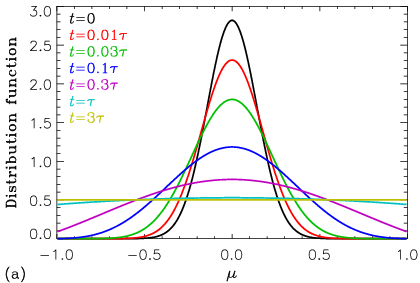
To illustrate the capabilities of the new codes, we have applied them to a particular type of non-factorizable electron distribution. We assume that energetic electrons are injected at large pitch angles and have initially a highly-anisotropic “pancake”-like distribution with a sharp peak at . Considering the pitch-angle scattering only, we can write the kinetic equation for the distribution function as (Fleishman & Toptygin 2013)

| (4) |
where the angular diffusion coefficient has the form
| (5) |
and is the scattering rate, which is reciprocal to the isotropization time . The distribution function changes with time as shown in Figure 1a, and becomes nearly isotropic at . Since the scattering rate is energy-dependent, the resulting pitch-angle distribution will be energy-dependent, too. For different conditions, this process can produce qualitatively different shapes of the electron distribution which are investigated below.
IV.1 Collisional scattering
Scattering due to collisions with the ambient particles has the following characteristics (Trubnikov 1965; Fleishman & Toptygin 2013, e.g.,):
| (6) |
where is the electron velocity, and and are the plasma density and temperature, respectively; i.e., the low-energy electrons are scattered more efficiently. An example for the energy dependence of the collisional scattering time (for and K) is shown in Figure 1b.
We have applied the pitch-angle scattering model (4) with the scattering time given by (6) and shown in Figure 1b to an electron distribution function that initially was described by the following (factorized) analytical expression:
| (7) |
in the energy range from MeV to MeV, with and ; this function represents a power-law distribution over energy and a symmetric loss-cone (or “pancake”) distribution over pitch-angle. We have assumed the integration time to be s, which is the minimum value of the scattering time in the considered energy range, or ). The resulting electron distribution function is shown in Figure 2a. Here, the electron distribution at the low-energy cutoff is almost isotropic, while at higher energies it retains a considerable anisotropy (equivalent to a loss-cone distribution with ).


The corresponding microwave spectra for two different viewing angles are shown in Figures 3–4; the spectra were computed within the continuous approximation (the harmonic structure at low frequencies is ignored). For comparison, we also show the simulation results for factorized electron distributions with the same pitch-angle profiles at all energies: the isotropic distribution and the loss-cone with (which are equivalent to the pitch-angle profiles of the non-factorized distribution function in Figure 2a at the low- and high-energy ends of the electron energy spectrum, respectively). One can see that the emission parameters for the non-factorized electron distribution are between those for the isotropic and loss-cone distributions; at higher frequencies, the emission parameters for the non-factorized electron distribution approach those for the loss-cone distribution. We note that the mentioned effect is noticeable in strong magnetic fields ( G) only; in weaker fields, the deviation from the loss-cone distribution is negligible because only the high-energy electrons make a contribution.


IV.2 Scattering on turbulence
In the presence of magnetic fluctuations, the mean free path of energetic electrons is often approximated by a power-law dependence on energy (Musset et al. 2018, e.g.,):
| (8) |
accordingly, the isotropization time is given by
| (9) |
Therefore, the high-energy electrons are scattered more efficiently. Musset et al. 2018 analyzed the X-ray and microwave source sizes in the 21 May 2004 flare (which were assumed to be determined by scattering of nonthermal electrons on turbulence) and estimated the corresponding scattering mean free path values as km at keV and km at keV; this corresponds to a power-law index of in Equation (8) if we associate the estimated mean free path with the turbulent one . The energy dependence of the turbulent scattering time is shown in Figure 1b.
We have applied the pitch-angle scattering model (6) with the scattering described by Equations (8–9) and estimations by Musset et al. 2018 (with the resulting scattering time shown in Figure 1b) to evolve the electron distribution function described initially by Equation (7) in the energy range from MeV to MeV, with and (note that the initial angular distribution is wider than in the previous example). We have adopted the integration time of s, which is the minimum value of the scattering time in the considered energy range, or ). The resulting electron distribution function is shown in Figure 2b. Here, the electron distribution at the high-energy end is almost isotropic, while at lower energies it retains a considerable anisotropy (equivalent to a loss-cone distribution with ).
The corresponding microwave spectra, again computed within the continuous approximation, for two different viewing angles are shown in Figures 5–6; for comparison, we also show the simulation results for factorized electron distributions with the same pitch-angle profiles at all energies: the isotropic distribution and the loss-cone with (which are equivalent to the pitch-angle profiles of the non-factorized distribution function in Figure 2b at the high- and low-energy ends, respectively). One can see that the emission parameters for the non-factorized electron distribution are again between those for the isotropic and loss-cone distributions; at higher frequencies, emission parameters for the non-factorized electron distribution approach those for the isotropic distribution. The mentioned effect is well visible for the typical coronal magnetic field strengths ( G).


IV.3 Spectral indices
Figures 7 and 8 demonstrate the spectral indices of microwave emission computed using the above models. The spectral index is defined as
| (10) |
The electron distribution functions and other source parameters in Figures 7 and 8 are the same as in Figures 3–4 and 5–6, respectively. In all cases, the spectral index computed from the kinetic solution differs measurably from those from the factorized approximations.
In the collision-dominated case (Figure 7), the spectral indices for the non-factorized distribution at high frequencies are not much different from those for the loss-cone distribution, because the high-energy electrons (which are still anisotropic, despite of collisions) make a dominant contribution to the microwave emission. The largest deviation from the loss-cone case occurs at intermediate frequencies (slightly above the spectral peak). We also note that, with frequency, for small viewing angles the spectral index for the non-factorized distribution approaches that for the loss-cone distribution from above, while for large viewing angles the spectral index for the non-factorized distribution approaches that for the loss-cone distribution from below.
In contrast, in the turbulence-dominated case (Figure 8), the spectral indices for the non-factorized distribution at high frequencies are more similar to those for the isotropic distribution. At small viewing angles, the optically thin spectral index for the non-factorized distribution is smaller (i.e., the spectrum is less steep) than that for the isotropic distribution, although this difference decreases with frequency. At large viewing angles, the differences between the considered electron distributions become very small but still noticeable: for the non-factorized distribution, the optically thin spectral index is larger (i.e., the spectrum is steeper) than those for the loss-cone and isotropic distributions.
V Discussion and Conclusions
In this paper we extend our fast GS codes (Fleishman & Kuznetsov 2010) to the case, where the distribution of the nonthermal electrons can be defined numerically in the form of two-dimensional arrays, describing the dependence of the nonthermal electrons on the energy and pitch-angle. Along with this feature, we made several other improvements and additions. In particular, we improved treatment of the free-free component following the theory of Fleishman et al. 2021c and permitted arbitrary user-defined list of frequencies where to compute the microwave emission.
The main development is the ability of the new codes to deal with the numerically defined distributions of the nonthermal electrons. This development paves the way for direct use of numeric solutions of acceleration/transport equations/codes to compute the observables such as the flux and polarization of the microwave emission.
Such solutions are now routinely obtained in numerical simulations of various levels of complexity—from ‘toy’ models, e.g. within a simple ‘escape time’ approximation (Fleishman 2006b) to sophisticated models, such as kglobal (Arnold et al. 2021), that take many important physical effects into account and permit arbitrary nonfactorized anisotropic distribution of the nonthermal electrons to be considered. The new codes offer the computation speed comparable to that of Fleishman & Kuznetsov 2010 supporting comparably fast computation of the microwave emission from rather large models.


References
- Arnold et al. (2021) Arnold, H., Drake, J. F., Swisdak, M., Guo, F., Dahlin, J. T., Chen, B., Fleishman, G., Glesener, L., Kontar, E., Phan, T., & Shen, C. 2021, Phys. Rev. Lett., 126, 135101
- Cohen (1960) Cohen, M. H. 1960, ApJ, 131, 664
- Eidman (1958) Eidman, V. Y. 1958, Soviet Phys. JETP, 7, 91
- Eidman (1959) —. 1959, Soviet Phys. JETP, 9, 947
- Fleishman (2006a) Fleishman, G. D. 2006a, ApJ, 638, 348
- Fleishman (2006b) Fleishman, G. D. 2006b, in Solar Physics with the Nobeyama Radioheliograph, 51–62
- Fleishman et al. (2021a) Fleishman, G. D., Anfinogentov, S. A., Stupishin, A. G., Kuznetsov, A. A., & Nita, G. M. 2021a, ApJ, 909, 89
- Fleishman et al. (2002) Fleishman, G. D., Fu, Q. J., Huang, G.-L., Melnikov, V. F., & Wang, M. 2002, A&A, 385, 671
- Fleishman et al. (2020) Fleishman, G. D., Gary, D. E., Chen, B., Kuroda, N., Yu, S., & Nita, G. M. 2020, Science, 367, 278
- Fleishman et al. (2021b) Fleishman, G. D., Kleint, L., Motorina, G. G., Nita, G. M., & Kontar, E. P. 2021b, ApJ, 913, 97
- Fleishman & Kuznetsov (2010) Fleishman, G. D. & Kuznetsov, A. A. 2010, ApJ, 721, 1127
- Fleishman et al. (2021c) Fleishman, G. D., Kuznetsov, A. A., & Landi, E. 2021c, ApJ, 914, 52
- Fleishman et al. (2017) Fleishman, G. D., Nita, G. M., & Gary, D. E. 2017, ApJ, 845, 135
- Fleishman et al. (2018) Fleishman, G. D., Nita, G. M., Kuroda, N., Jia, S., Tong, K., Wen, R. R., & Zhizhuo, Z. 2018, ApJ, 859, 17
- Fleishman et al. (2016) Fleishman, G. D., Pal’shin, V. D., Meshalkina, N., Lysenko, A. L., Kashapova, L. K., & Altyntsev, A. T. 2016, ApJ, 822, 71
- Fleishman & Toptygin (2013) Fleishman, G. D. & Toptygin, I. N. 2013, Cosmic Electrodynamics (Springer, New York)
- Gary et al. (2018) Gary, D. E., Chen, B., Dennis, B. R., Fleishman, G. D., Hurford, G. J., Krucker, S., McTiernan, J. M., Nita, G. M., Shih, A. Y., White, S. M., & Yu, S. 2018, The Astrophysical Journal, 863, 83
- Gordovskyy et al. (2019) Gordovskyy, M., Browning, P., & Pinto, R. F. 2019, Advances in Space Research, 63, 1453
- Gordovskyy et al. (2017) Gordovskyy, M., Browning, P. K., & Kontar, E. P. 2017, A&A, 604, A116
- Klein (1987) Klein, K.-L. 1987, A&A, 183, 341
- Kuroda et al. (2018) Kuroda, N., Gary, D. E., Wang, H., Fleishman, G. D., Nita, G. M., & Jing, J. 2018, ApJ, 852, 32
- Kuznetsov & Fleishman (2021) Kuznetsov, A. & Fleishman, G. 2021, Ultimate fast gyrosynchrotron codes: the first release
- Li & Fleishman (2009) Li, Y. & Fleishman, G. D. 2009, ApJ, 701, L52
- Melrose (1968) Melrose, D. B. 1968, Ap&SS, 2, 171
- Motorina et al. (2020) Motorina, G. G., Fleishman, G. D., & Kontar, E. P. 2020, ApJ, 890, 75
- Musset et al. (2018) Musset, S., Kontar, E. P., & Vilmer, N. 2018, A&A, 610, A6
- Nita et al. (2015) Nita, G. M., Fleishman, G. D., Kuznetsov, A. A., Kontar, E. P., & Gary, D. E. 2015, ApJ, 799, 236
- Nita et al. (2018) Nita, G. M., Viall, N. M., Klimchuk, J. A., Loukitcheva, M. A., Gary, D. E., Kuznetsov, A. A., & Fleishman, G. D. 2018, ApJ, 853, 66
- Petrosian (1981) Petrosian, V. 1981, ApJ, 251, 727
- Press et al. (2002) Press, W. H., Teukolsky, S. A., Vetterling, W. T., & Flannery, B. P. 2002, Numerical recipes in C++ : the art of scientific computing (Cambridge University Press, Cambridge)
- Ramaty (1969) Ramaty, R. 1969, ApJ, 158, 753
- Trubnikov (1965) Trubnikov, B. A. 1965, Reviews of Plasma Physics, 1, 105
- Waterfall et al. (2019) Waterfall, C. O. G., Browning, P. K., Fuller, G. A., & Gordovskyy, M. 2019, MNRAS, 483, 917
- Waterfall et al. (2020) Waterfall, C. O. G., Browning, P. K., Fuller, G. A., Gordovskyy, M., Orlando, S., & Reale, F. 2020, MNRAS, 496, 2715
- Wild & Hill (1971) Wild, J. P. & Hill, E. R. 1971, Australian Journal of Physics, 24, 43
- Zheleznyakov & Zlotnik (1964) Zheleznyakov, V. V. & Zlotnik, E. Y. 1964, Soviet Ast., 7, 485
Appendix A On the interpolation
The numerically-defined electron distribution function is specified by a 2D array of values at the nodes of a regular grid given by and . To compute the gyrosynchrotron emission, we need to know the function values , together with its derivatives over energy and pitch-angle and (for the continuous gyrosynchrotron approximation) the second derivative over pitch-angle , at arbitrary points in the energy-pitch-angle space. For this, we use two different interpolation methods.
2D cubic spline interpolation
The classical implementation of 1D cubic spline interpolation (Press et al. 2002, see, e.g.,) implies that at any interval , the interpolated function is given by a local cubic polynomial depending on the specified function values at the adjacent grid nodes and and on the second derivatives of the function at the same nodes and ; the second derivatives at all nodes are computed globally (before the interpolation) using the specified function values at the nodes, by solving a system of equations. Accordingly, the first and second derivatives of the interpolated function and are given by local quadratic and linear polynomials, respectively. In our code, the 2D spline interpolation is implemented in the following way: at the initialization step, before the interpolation, we construct a number of 1D splines, i.e.
- 1.
For each column of the input array (i.e., for ), we construct a spline describing the pitch-angle dependence of the distribution function , and compute the second derivative values at the grid nodes.
- 2.
For each row of the input array (i.e., for ), we construct a spline describing the energy dependence of the distribution function , and compute the second derivative values at the grid nodes.
- 3.
Using the results of the previous step, for each column of the input array, we construct a spline describing the pitch-angle dependence of the second derivative of the distribution function over energy and compute the fourth derivative values at the grid nodes.
At the boundaries of the array, the first derivatives of the 1D spline functions are assumed to be equal those derived using three-point Lagrange interpolation—this approach was found to provide the most accurate results.
At each point , such that and , the interpolation is performed in two steps. Firstly, we interpolate over pitch-angle , i.e., compute the values of the distribution function and its derivatives at the points and :
- 1.
Using the values , , , and , and the 1D spline formulae, we compute the interpolated values of the distribution function , as well as of its derivatives over pitch-angle and .
- 2.
Using the values , , , and , and the 1D spline formulae, we compute the interpolated values of the second derivative of the distribution function over energy , as well as of its derivatives over pitch-angle and .
Similarly, we compute the corresponding interpolated values at : , , , , , and . Then we perform interpolation over energy , i.e.
- 1.
Using the values , , , and , and the 1D spline formulae, we compute the interpolated values of the distribution function and of its derivative .
- 2.
Using the values , , , and , and the 1D spline formula, we compute the interpolated values of the first derivative of distribution function over pitch-angle .
- 3.
Using the values , , , and , and the 1D spline formula, we compute the interpolated values of the second derivative of distribution function over pitch-angle .
Linear-quadratic 2D interpolation
In contrast to the previous case, this is a local approach, when the interpolated function values are determined by its values at several (four or six) adjacent nodes. The distribution function itself is computed using bilinear interpolation. The derivatives and are computed using a linear interpolation in one variable and a Lagrange interpolation on three closest points in another variable (where the derivative is needed).
By default, we use the 2D cubic spline interpolation, because it usually provides a higher accuracy and speed (due to a higher smoothness of the interpolated function, the numerical routines converge faster). However, due to its global nature, this approach can produce undesirable artifacts (“wiggles” on the interpolated function) when applied to distributions with very sharp gradients; in particular, a maser instability can occur even if the numerically-defined distribution function has no positive slope (but has a very steep negative slope somewhere). In this respect, the linear-quadratic interpolation is more stable.
Another important feature related to interpolation is the grid spacing. Since the electron distributions in the solar corona can cover a wide range of energies, logarithmically-spaced grids () are usually used to describe them. To improve the interpolation accuracy, in such cases we interpolate not the dependence of vs. , but the dependence of vs. ; for a power-law distribution, both the spline and linear-quadratic interpolation methods provide exact results in this case. A disadvantage of this approach is that the distribution function array must not contain zero values. We offer a user the opportunity to switch between the vs. (suitable for logarithmically-spaced grids, used by default) and vs. (suitable for equidistant grids) interpolation regimes, according to their model. For the pitch-angle distributions, no variable substitutions are used, i.e., an equidistant grid over would provide the best results. We note that the values of should cover the entire range of possible values (i.e., and ); otherwise, extrapolation beyond the specified range can occur during computations, which will reduce the accuracy greatly.