A Snowball in Hell: The Potential Steam Atmosphere of TOI-1266cJournal: PSJAtmos (Arney et al. 2017), Planetary Spectrum Generator (PSG) (Villanueva et al. 2018)
Abstract
TOI-1266c is a recently discovered super-Venus in the radius valley orbiting an early M dwarf. However, its notional bulk density (2.2 g cm-3) is consistent with a large volatile fraction, suggesting that it might have volatile reservoirs that have survived billions of years at more than twice the Earth’s insolation. On the other hand, the upper mass limit paints a picture of a cool super Mercury dominated by >50% iron core (9.2 g cm-3) that has tiptoed up to the collisional stripping limit and into the radius gap. Here, we examine several hypothetical states for TOI-1266c using a combination of new and updated open-source atmospheric escape, radiative-convective, and photochemical models. We find that water-rich atmospheres with trace amounts of H2 and CO2 are potentially detectable (SNR ) in less than 20 hours of JWST observing time. By prescribing high altitude water and ice clouds, weWe also find that water vapor spectral features are not substantially impacted by the presence of high-altitude water or ice clouds due the presence of a significant amount of water above the cloud-deck, although further work with self-consistent cloud modelingmodels is needed. Regardless of its mass, however, TOI-1266c represents a unique proving ground for several hypotheses related to the evolution of sub-Neptunes and Venus-like worlds, particularly those near the radius valley.
Keywords:
Exoplanet atmospheres (487), Hot Neptunes (754), Extrasolar ice giants (2024), Extrasolar rocky planets (511), Exoplanets (498), Star-planet interactions (2177), Super Earths (1655), Exoplanet atmospheric composition (2021)I Introduction
The list of exoplanet detections from space-based observatories like the Kepler Space Telescope (Borucki et al. 2010; Twicken et al. 2016, e.g.,) and the Transiting Exoplanet Survey Satellite (Ricker et al. 2014; Barclay et al. 2018, TESS;), as well as ground-based endeavors such as WASP (Pollacco et al. 2006, e.g.), HATNet (Bakos et al. 2004; Hellier et al. 2012, e.g.), TRAPPIST (Jehin et al. 2011; Gillon et al. 2017; Delrez et al. 2018), and the Habitable-zone Planet Finder (HPF) Spectrograph (Mahadevan et al. 2012; Mahadevan et al. 2014), is rapidly growing. These detections enhance our understanding of planetary occurrence rates (Batalha 2014) as well as enable robust statistical insights into planet populations (Dressing & Charbonneau 2013; Burke et al. 2015; Fulton et al. 2017; Hardegree-Ullman et al. 2019, e.g.,). In particular, the presence of a gap in the radius distribution of planets (Rogers 2015; Fulton et al. 2017; Fulton & Petigura 2018) highlights the cumulative effects of a planet’s host star (Owen & Jackson 2012; Owen & Wu 2017, e.g.,), formation (Lee et al. 2014; Lee & Chiang 2016; Ginzburg et al. 2018; Gupta & Schlichting 2020, e.g.,), and/or evolution (Luger et al. 2015, e.g.,), although disentangling these effects will likely require more sensitive observations (Loyd et al. 2020).
The recent discovery of two planets orbiting TOI-1266 (Stefansson et al. 2020; Demory et al. 2020) offers a rare opportunity to begin connecting some of these planetary processes through observations. The outer planet, c (1.673 R⊕); 1.56R⊕) (using published radius parameters and 1- uncertainties from Stefansson et al. 2020 and Demory et al. 2020, respectively), is smaller than the inner planet, b (2.458 R⊕) (see Table 1 for the reported uncertainties and a comparison between the Stefansson et al. 2020 and Demory et al. 2020 values); 2.37 R⊕) (Stefansson et al. 2020; Demory et al. 2020). This puts TOI-1266c in the ‘radius valley’ (Fulton et al. 2017; Fulton & Petigura 2018). This type of ‘straddler’ planetary system (Owen & Campos Estrada 2020) can be leveraged to constrain the temporal evolution of host star’s EUV flux, but. However, the flipped orientation (withfact that the smaller planet to theis outside of the larger one (Weiss et al. 2018) hints at significant migration that may obfuscatedefeat first-order attempts to reproduce their present-day bulk compositions through atmospheric escape alone (Bean et al. 2021).
The mass of planet c hasbulk composition of TOI-1266c is poorly constrained because the mass measurement has large 1- uncertainties (1.9 and 2.2 M⊕, again from Stefansson et al. 2020 and Demory et al. 2020, respectively): 1.9 M⊕ from Stefansson et al. 2020 using radial velocity constraints, and 2.2 M⊕ from Demory et al. 2020 based on an analysis of the transit timing variations. This broad range of possible planet masses covers several different planet types including both rocky terrestrials and gas-dominated sub-Neptunes. Currently, compositional constraints are insufficient to rule out significant volatile inventories for small exoplanets under even higher instellation than what planet c receives (Dai et al. 2019). Formation models suggest that sub-Neptunes/super-Earths like TOI-1266b and c can end up as part of distinct water- or silicate-rich populations if planet embryos aggregate material from a more well-sampled protoplanetary disk (Liu et al. 2019, e.g.). It may also be easier to form volatile-rich mini-Neptunes if additional gas sources, such as envelope enrichment sourced from various accreted ices, are considered (Venturini & Helled 2017, e.g.). Taken together, TOI-1266c may becould be a rare example of a volatile-rich super-Earth, contrasting with the more well-populated family of volatile-poor, rocky super-Earths such as LHS 3844b (Kane et al. 2020) and TOI-849b (Armstrong et al. 2020).
| Property | Stefansson et al. 2020 | Demory et al. 2020 |
|---|---|---|
| TOI-1266: | ||
| Spectral type | M2 | M3 |
| Mass [M⊙] | 0.437 0.021 | 0.45 0.03 |
| Radius [R⊙] | 0.4232 | 0.42 0.02 |
| Temperature [K] | 3563 77 | 3600 150 |
| Age [Gyr] | 7.9 | 5 |
| Luminosity [L⊙] | 0.02629 | — |
| Planet b: | ||
| Mass [M⊕] | 6.9 | 13.5 |
| Radius [R⊕] | 2.458 | 2.37 |
| Semi-major axis [au] | 0.0745 | 0.0736 |
| Instellation [S⊕] | 4.72 | 4.9 |
| Equilibrium temp.∗ [K] | 410.0 | 413 20 |
| Planet c: | ||
| Mass [M⊕] | 1.9 | 2.2 |
| Radius [R⊕] | 1.673 | 1.56 |
| Semi-major axis [au] | 0.1037 | 0.1058 |
| Instellation [S⊕] | 2.42 | 2.3 |
| Equilibrium temp.∗ [K] | 347.1 | 344 16 |
In this paper, we explore the potential states of the planet by focusing on the H-C-O chemistry of three families of scenarios, all dominated by water: H2+H2O, H2+CO2+H2O, and O2+H2O. This encompasses two potential intermediate states (as we describe below) as well as a hypothetical super-Venus transitional state, in which CO2 begins to represent a significant portion of the envelope mass. We omit two other classes of atmospheres (Venus-like and sub-Neptune) for the sake of brevity. Simulations of exo-Venus atmospheres (Schaefer & Fegley Jr 2011; Lincowski et al. 2018; Lustig-Yaeger et al. 2019a) largely resemble Venus’ CO2-dominated atmosphere at present or with smaller CO2 inventories earlier in its history (Way & Del Genio 2020, e.g.). For exo-Venuses in particular, more exploration is warranted to cover the expected diversity of planetary conditions and composition (Madhusudhan et al. 2016, see the review by). A number of studies on the diversity of sub-Neptune atmospheres (Lavvas et al. 2019; Chouqar et al. 2020, e.g.,) and retrievals (Benneke et al. 2019; Mikal-Evans et al. 2020, e.g.,) can be found in the literature; see also the review by Bean et al. 2021.
But estimating the composition and any potential observables for TOI-1266c remains difficult. The degeneracies in relating bulk composition, atmosphere-to-solid planet fraction, and mean density (Rogers & Seager 2010; Dorn et al. 2015; Welbanks & Madhusudhan 2019, e.g.) pose significant challenges in predicting the atmospheres of exoplanets even if the mass and radius are well constrained, and even spectroscopic observations of the planet may not necessarily break this degeneracy (Batalha et al. 2017a). Additional radial velocity observations–such as precision RVs with HPF (Mahadevan et al. 2012; Mahadevan et al. 2014), NEID or CARMENES–are required to constrain the planet’s mass, which will narrow the range of possible compositions (Valencia et al. 2013, e.g.), but in the meantime we can begin exploring the connections between composition, evolution, and observations.

I.1 Motivating the ‘snowball’ scenario
The current mass of TOI-1266c affords a variety of different possible compositions that largely fork into two main solutions: a water-rich steam world, and a dense Mercury-like planet. As shown by Stefansson et al. 2020, TOI-1266c is broadly consistent with a water-dominated planet (Aguichine et al. 2021, Fig. 1; see also). This can be seen when comparing to modeled mass-radius relationships for more complex compositions. For example, the radius estimates for an Earth-like planet surrounded by up to 50 wt% (percent water by mass) yieldcan have radii of up to 1.47 R⊕ (Fu et al. 2009), which is 12% smaller than the observed radius for TOI-1266c (though this is still within 2). As an intermediate step, tThe model grid from Zeng et al. 2019 includes aseveral 50% water/Earth-like rocky core planets with a 1,000 K isothermal pure-H2O atmospheres that roughly matches TOI-1266c’s mass and radius. Moving away from an ‘Earth-like’ composition, the genericMore generalized formulations for ice/rock/iron fractional compositions of Fortney et al. 2007 suggests that TOI-1266c is % water ice by mass, while the model from Noack et al. 2016 suggests a lower limit of 77 wt-% H2Osuggest that TOI-1266c is 60% water ice (Fortney et al. 2007) or 77% liquid water (Noack et al. 2016) by mass., with only a 50 km radius difference if the remaining fraction is iron or silicates. These estimates are comparable to the maximum ice content expected for planets formed beyond the ice line (Mordasini et al. 2009, e.g.), suggesting that in this scenario, both planet b and c migrated inwards to their present locations. However, none of these mass-radius relationships have self-consistent atmospheres, which can lead to underestimates in the estimated radius (Turbet et al. 2020, e.g.,). Given TOI-1266c’s current equilibrium temperature of 250 K, assuming an albedo0.3, it is unlikely that there is a substantial supercritical water component, and instead, TOI-1266c is ‘liquid’ water-dominated (Brugger et al. 2017; Mousis et al. 2020b).
Such sSteam atmospheres are often discussed within the context of the loss of water either during the magma ocean phase of a planet, immediately following accretion (Zahnle et al. 1988; Schaefer & Fegley Jr 2010; Hamano et al. 2013; Katyal et al. 2019, e.g.,) or as a result of stellar brightening inducing a runaway greenhouse state (Kasting 1988, e.g.). However, abundant water (and other heavy gases) cancould also be accreted (Kral et al. 2020) or outgassed later in a planet’s life (Kite et al. 2020; Kite & Barnett 2020; Kite & Schaefer 2021), potentially setting up a scenario in which the runaway state is entered much later in the planet’s life.
One unavoidable consequence of a potentially water-dominated planet receiving slightly more irradiation than Venus is atmospheric escape. Venus is thought to have lost its water at some point in its history (Kasting 1988; Way & Del Genio 2020, e.g.,) due to high temperatures allowing significant amounts of water in the upper atmosphere, where it could be photolyzed and create hydrogen atoms that then escape the atmosphere (Kasting & Pollack 1983, e.g.,). A high hydrogen escape flux would also drag along oxygen (Zahnle & Kasting 1986; Schaefer et al. 2016; Luger & Barnes 2015; Tian 2015, e.g.,). Of particular note for M dwarfs is their prolonged pre-main sequence lifetimes, during which they are 10-100 times brighter than their main sequence luminosities (Luger & Barnes 2015; Luger et al. 2015). As a result, planets like TOI-1266c have multiple avenues by which their atmospheric composition can evolve in time, even to the extent that the planet loses its atmosphere entirely (Kreidberg et al. 2019; Poppenhaeger et al. 2020, e.g.). A second issue is that planets orbiting M dwarfs may be volatile-poor due to the high impact velocities during formation (Lissauer 2007, e.g.,). However, if the planet began with larger initial volatile inventories (Luger et al. 2015, e.g.), replenished its atmospheric volatiles through regassing from the interior (Moore & Cowan 2020, e.g.), or experienced slower than expected atmospheric escape, TOI-1266c may still have a substantial envelope today.
On the other extreme, the 2- upper mass limit of 6.4 M⊕ for TOI-1266c would indicate that the planet is >50% iron core (Noack et al. 2016, following the mass-radius relationship given by), near the size limit driven by collisional stripping from impacts during accretion (Marcus et al. 2010). TOI-1266c would then represent a super Mercury at less than half of Mercury’s instellation, which would have implications for the composition of its atmosphere. At lower planetary masses, TOI-1266c would likely still have an iron core but could also have a modest H2-He envelope, on the order of 0.2-0.5% of the total planet mass (Lopez & Fortney 2014; Zeng et al. 2019).
However, twoseveral theoretical arguments work to rule outmake it difficult to form an iron core with a substantial H2-He fraction. First, a gas-rich initial composition is inconsistent with rocky planet formation models, which suggest that substantial accumulation of H2 and He from the protoplanetary disk requires a minimum core mass 5-20 M⊕ (Rafikov 2006; Rafikov 2011, e.g.,). Additionally, pPlanets with small rocky cores are also subject to atmospheric ‘boil-off’ supported by the planet’s inability to cool rapidly enough (Owen & Wu 2016), potentially followed by loss driven by the cooling of the core (Misener & Schlichting 2021, e.g.) and/or photo-evaporation (Owen & Wu 2017, e.g.). Boil-off would prevent the accumulation of more than a few tenths of a percent H2, even if the planet began with 10% by mass H2 (Owen & Wu 2016), given the high equilibrium temperature for TOI-1266c during the super-luminous pre-main sequence phase of the host star (Luger & Barnes 2015, e.g.,), assuming it was in its present location. Core-powered mass loss and photoevaporation would further reduce the amount of H2, ultimately leaving behind an evaporated core (Luger et al. 2015) that would be inconsistent with current mass and radius constraints for TOI-1266c. These arguments effectively rule out a H2-dominated state, although it is important to note that more complex models of the mass and radius evolution of volatile-rich planets still suggest a peak for planets with 1% H2/He atmospheres (Chen & Rogers 2016). Additionally, secondary loss processes like ion pickup could further modify the atmosphere (see Gronoff et al. 2020, for an overview), although the stellar wind for TOI-1266 is only modest at present ( M⊙/yr, based on rotation constraints) (Johnstone et al. 2015a).
We can combine this with the limited information we have about the solar system giants. Uranus and Neptune have interior ‘high-metallicity’ (elements heavier than He) components ranging from 75-90% of the their total mass, depending on whether silicates and/or ices are assumed to be the ’metal’ (Hubbard 1981; Helled et al. 2010, e.g.,). This is consistent with other estimates regarding the internal composition of sub-Neptune-sized exoplanets (Wolfgang & Lopez 2015, e.g.,). This translates to roughly 11-13 and 13-15 M⊕ for Uranus and Neptune, respectively (Helled et al. 2010; Dodson-Robinson & Bodenheimer 2010), larger than the 2- upper bound on TOI-1266c’s mass estimate. The ice component (Hubbard 1981, thought to be the majority of the core;) is expected to be of supersolar metallicity (Lodders & Fegley Jr 1994), with Neptune having a higher oxygen-to-hydrogen fraction (corresponding to a higher water ice fraction). This wcould also push the C/O ratio to higher values, approaching 1 (Ali-Dib et al. 2014, see also the review by Mousis et al. 2020a, Mousis et al. 2020a), although sSeveral studies have motivated C/O ratios closer to 0.5 and a modest amount of ammonia ice (Nettelmann et al. 2016), which would be physically consistent with protoplanetary material that experienced full clathration (Mousis et al. 2020a). This is further complicated by the fact that assumptions about atmospheric structure and what type of adiabat the temperature profile follows (ranging from dry to wet) shift the retrieved atmospheric metallicity by a factor of a few (Cavalié et al. 2017).
Taken together, there is a compelling case to assume that TOI-1266c is volatile-rich, and may even be an eroded sub-Neptune core. We take CO2 as the major carbon-bearing species, as the CO/CH4 transition and the CO2 fraction peak at intermediate temperatures and pressures for higher-metallicity atmospheres (Lodders & Fegley Jr 2002; Venot et al. 2014); likewise, N2 dominates over NH3 (Burrows & Sharp 1999). We can begin exploring the potential states of the planet by focusing on the H-C-O chemistry of three families of scenarios, all dominated by water: H2+H2O, H2+CO2+H2O, and O2+H2O. This encompasses two of the potential intermediate states (where H2 is still present, or when water has been lost and O2 is accumulating) as well as a hypothetical super-Venus transitional state, in which CO2 begins to represent a significant portion of the envelope mass. We can further motivate the choice of CO2 as the major carbon-bearing species with work suggesting that the CO/CH4 transition and the CO2 fraction peak at intermediate temperatures and pressures for higher-metallicity atmospheres (Lodders & Fegley Jr 2002; Venot et al. 2014); likewise, N2 dominates over NH3 (Burrows & Sharp 1999). In this paper, we focus on steam atmospheres, omitting two classes of atmospheres (Venus-like and sub-Neptune) for the sake of brevity. Simulations of exo-Venus atmospheres (Schaefer & Fegley Jr 2011; Lincowski et al. 2018; Lustig-Yaeger et al. 2019a) largely resemble Venus’ CO2-dominated atmosphere at present or with smaller CO2 inventories earlier in its history (Way & Del Genio 2020, e.g.). For exo-Venuses in particular, more exploration is warranted to cover the expected diversity of planetary conditions and composition (Madhusudhan et al. 2016, see the review by). A number of studies on the diversity of sub-Neptune atmospheres (Lavvas et al. 2019; Chouqar et al. 2020, e.g.,) and retrievals (Benneke et al. 2019; Mikal-Evans et al. 2020, e.g.,) can be found in the literature; see also the review by Bean et al. 2021.
II Methods
We use a one-dimensional radiative-convective cloud-free model from Kopparapu et al. 2013; Kopparapu et al. 2014, which was updated from the original version (Kasting 1988; Kasting et al. 1993) with new H2O and CO2 absorption coefficients. We employ inverse climate calculations in which the vertical temperature profile is specified, and radiative fluxes from the planet are back-calculated to determine the equivalent incident stellar flux. The atmosphere is divided into 101 layers. The model uses a moist pseudoadiabat extending from the “surface” (assumed to be at 100 bar) up to an isothermal stratosphere of 200 K. The surface temperature is varied until the effective solar flux () matches the observed incident flux on the planet. S is calculated from the ratio between the net outgoing IR flux (F) and the net incident solar flux (F), both evaluated at the top of the atmosphere. Essentially, by changing the surface temperature to match the incident stellar flux in our model, we are making sure that energy balance is maintained. The model top pressure is set to 10 bar bar. Short-wave and long-wave fluxes are calculated using a -2-stream approximation (Toon et al. 1989) using separate eight-term, correlated-k coefficients for H2O.
We also use a one-dimensional photochemical model that is a fork of Atmos11 1 Atmos on GitHub (Arney et al. 2017) with a modified version of the C-H-O photochemical network from VULCAN22 2 VULCAN on GitHub (Tsai et al. 2017, see Appendix A). We deliberately set aside nitrogen chemistry for this study because of both the additional complexity necessary to include it in our model, as well asand because of the uncertainties associated with speciation (we will return to this briefly in Section IV.1). Initial tests with a 0-dimensional chemical equilibrium model suggest that in the relatively oxidizing water-dominated scenarios we explore here, nitrogen is largely present as N2, which would contribute to a higher mean molecular weight for the atmosphere but have few other practical impacts. The atmosphere is assumed to be well-mixed below the ‘surface’ at 100 bars. The model also includes newly-measured water vapor photolysis cross sections (Ranjan et al. 2020). We use the ultraviolet through near-infrared spectra for GJ 581 (France et al. 2016; Youngblood et al. 2016; Loyd et al. 2016) as a proxy for TOI-1266, as they have comparable effective temperatures, luminosities, and ages, within uncertainties (Selsis et al. 2007; Dragomir et al. 2012; Gaia Collaboration et al. 2018). GJ 581 is technically a variable star, but its brightness variations are relatively small1% (Dragomir et al. 2012).
WeIn our photochemical simulations, we ensure that the total mixing ratio is unity by using He as the remainder of the atmosphere. The amount of He added is generally 1% by volume. As an aside, He abundances could be reduced by drag-off if escape fluxes are high, but we find using another gas (such as Ar) for this purpose has no qualitative impact on our photochemical results. We have also chosen a vertical eddy diffusion parameter K cm2/s consistent with other preliminary studies of hot Jupiters (Venot et al. 2014, e.g.,), noting that we have no constraints on the internal heat flux, rotation rate, and magnetic field strengths in order to constrain this value (e.g., Visscher et al. 2010, and references therein). We explore the effect of differing K later, but to first order, lower values of K decrease the vertical extent of the well-mixed region of the atmosphere, but do not significantly impact the results described below.
Given TOI-1266c’s current equilibrium temperature (see Table 1), it is unlikely that there is a substantial supercritical water component, and instead, TOI-1266c is ‘liquid’ water-dominated (Brugger et al. 2017; Mousis et al. 2020b). While the lower atmospheres in all of the cases we present here are above the critical temperature of water, the upper atmosphere passes through the temperature range where water would normally condense. We include in our calculations an updated H2O saturation vapor pressure over water and ice (Meyer et al. 1983; Haar et al. 1984), and moderate the condensation loss frequency to ensure that the atmosphere is not substantially supersaturated where liquid water can condense (233 K), and below this the condensation over ice is allowed to decrease, reflecting higher possible supersaturations (Wallace & Hobbs 2006; Korolev & Mazin 2003), consistent with observations of cirrus clouds on Earth (Krämer et al. 2009, e.g.,). This is in keeping with other studies of temperate water-dominated atmospheres (Piette & Madhusudhan 2020, e.g.,). We do not, however, include either aerosols to serve as cloud condensation nuclei nor the necessary microphysical models to capture cloud formation processes, nor the radiative effects of clouds, and caution that the estimated cloud properties are solely illustrative. We return to this later in the Section IV.
One additional constraint on the composition of the atmosphere is the cumulative impact of historic X-ray () and extreme ultraviolet () radiation-driven mass loss (the sum is represented as ). To do this, we have developed a simple model of atmospheric loss33 3 GitHub repository for Snowball separate from the other two models. The escape model interpolates the BaSTI luminosity evolution grid44 4 http://basti-iac.oa-abruzzo.inaf.it/ of Hidalgo et al. 2018 to the observed mass and luminosity of the host star (see Fig. 2, top panel), similar to Barnes et al. 2020. The stellar luminosity evolution of Hidalgo et al. 2018 agrees with other stellar evolution models (Baraffe et al. 2015) from 0.01-10 Gyr (the interval for the Baraffe et al. 2015 grid), and include time points back to 0.01 Myr and out to the end of the main sequence, even if this is beyond the age of the universe. Given the large uncertainty in the age of TOI-1266, this larger stellar age range allows for a more complete uncertainty analysis. We then use the X-ray and EUV scaling relationships from Peacock et al. 2020 (see Fig. 2, bottom panel), rather than the empirical scaling with respect to the bolometric luminosity (L) from Sanz-Forcada et al. 2011, for two reasons. First, the EUV luminosity (L) from Sanz-Forcada et al. 2011 is above 1% of L for 0.2 Gyr, and above 0.1% for over 1 Gyr, due to the lack of an EUV saturation threshold for younger stars. The second issue with using the parameterizations of Sanz-Forcada et al. 2011 is that for a dimmer star like TOI-1266, there is a discontinuity in the calculated X-ray luminosity (L) saturation timescale (0.33 Gyr) using their Equation 5, such that the post-saturation L is briefly higher than it is in the saturated regime. During our initial tests, we chose to empirically set the saturation timescale to when the time-dependent X-ray luminosity falls below the saturated value, resulting in 0.47 Gyr, which produced a negligible change in the total mass lost. We instead chose to use the X-ray and EUV scaling relationships from Peacock et al. 2020 in order to address these two discrepancies. Peacock et al. 2020 note a saturation of 10-2 F/F in their simulations of 0.4 M⊙ stars, slightly higher in magnitude but qualitatively consistent with work for larger stars (King & Wheatley 2020, e.g.,). Additionally, the log-linear dependence on age after the saturated period is comparable with other early M dwarf studies (Stelzer et al. 2013, e.g.,). These specific values from Peacock et al. 2020 are converted from flux ratios to luminosity ratios using the luminosity, distance, and 2MASS J-band magnitude listed in Stefansson et al. 2020, assuming that the J-band fluxes are proportional to the bolometric luminosity55 5 Changes in stellar effective temperature are 10% for 0.4-0.5 M⊙ stars over their lifetimes (Baraffe et al. 2015; Hidalgo et al. 2018), which would shift the wavelength peak by ¡50 nm..

Our escape model also takes advantage of the parameterizations available to distinguish between the radiation/recombination-, energy-, photon-, and diffusion-limited escape regimes (Murray-Clay et al. 2009; Owen & Alvarez 2016; Lopez 2017). This is not strictly necessary, given the intermediate XUV fluxes experienced by TOI-1266c,as the XUV fluxes at TOI-1266c are much less than those experienced by hot Jupiters thought to be undergoing radiation/recombination-limited escape. (Murray-Clay et al. 2009). butHowever, depending on our choices for the mass loss efficiency (a.k.a., the heating efficiency), atmospheric composition, and XUV luminosity saturation, the atmosphere transitions into these different escape regimesbetween the energy-, photon-, and diffusion-limited escape regimes at different times.
We also assume that our escape calculations are largely insensitive to exospheric temperature, except for across the critical XUV flux identified for hot Jupiters (Koskinen et al. 2007). This is motivated by the interesting coincidence of the critical XUV flux necessary to drag off atomic oxygen from a terrestrial planet’s atmosphere (Luger & Barnes 2015, 40 times the XUV flux received by Earth today;) and the XUV flux at which H cooling becomes ineffective at moderating thermospheric temperatures for gas giants (Koskinen et al. 2007). For gas giants, this transition produces an order of magnitude increase in the thermospheric temperature and atmospheric scale heights (Koskinen et al. 2007, their Fig. 1a). Temperature changes are accurately assessed as a secondary effect in the critical XUV flux relationship for planets in their host star’s main sequence habitable zone shown by Luger & Barnes 2015, since the critical XUV flux goes as T-1/4. However, including a 10 change in temperature would cause the critical XUV flux to decrease by more than a factor of two (that is, the onset of oxygen drag-off would occur at lower fluxes). For habitable zone planets like those studied by Luger & Barnes 2015 and Ramirez & Kaltenegger 2014, this assumption does not introduce significant errors over the 1 Gyr that these planets spend enduring the superluminous phase of their host stars. As we focus on water-dominated scenarios, the prevalence of molecular hydrogen and oxygen in the thermosphere suggests a closer resemblance to the upper atmosphere of Earth or Jupiter (1,000-2,000 K) than the CO2-dominated atmospheres of Venus and Mars (Mueller-Wodarg et al. 2008, 200-300 K;), but under high instellation, even CO2-dominated thermospheres are 10,000 K (Tian 2009). This, combined with the potential for Lyman- cooling at high XUV fluxes (Murray-Clay et al. 2009, e.g.,), suggests that above 180 erg cm-2 s-1 the exospheric temperature is 10,000 K, and 1,000 K below this flux threshold. Since TOI-1266c receives >180 erg cm-2 s-1 for nearly 3.5 Gyr, we find that escape of atomic oxygen continues for 2 Gyr longer than if we were to adopt the critical XUV flux suggested by Luger & Barnes 2015 of 400 erg cm-2 s-1 for a planet with TOI-1266c’s current mass and radius. This results in lower potential for accumulated oxygen abundances in nearly every scenario for TOI-1266c, consistent with prior work that demonstrated oxygen accumulation and escape self-consistently for XUV fluxes 10-100 times larger than what the Earth receives today (Zahnle & Kasting 1986, Fig. 2; e.g.,).
We assume mass loss efficiencies () in line with other authors, including 0.1-0.15 for X-ray-dominated H2 escape for a planet of comparable size to TOI-1266c (Owen & Jackson 2012; Bolmont et al. 2017), and 0.01 for H2O following Lopez 2017, based on protoplanetary disk photoevaporation studies (Ercolano & Clarke 2010). These are meant only as order-of-magnitude approximations, since the efficiency is dependent on planetary mass, radius, and envelope composition and its radiative properties, as well as the flux of high-energy radiation from its host star, and as such will evolve (Murray-Clay et al. 2009; Owen & Wu 2013, e.g.,). A planned next step is to use the flux-dependent efficiencies of Bolmont et al. 2017, noting that there is still some uncertainty when comparing these to efficiencies for close-in giant planets (Koskinen et al. 2014, e.g.,).
Because of the inherent uncertainties associated with almost every aspect of the atmospheric escape as well as the planet’s mass and composition, we employ a Monte Carlo approach and perform a suite of escape simulations over the range of parameter uncertainties set out in Table 2. The atmospheric composition values are drawn from a log-uniform distribution, whereas all other values are drawn from linear uniform ranges. Values are selectedgenerated using the Latin Hypercube sampling (LHS) method in the Surrogate Modeling Toolbox (Bouhlel et al. 2019), which leverages the Enhanced Stochastic Evolutionary algorithm (Jin et al. 2003) to optimize the Design of Experiments Toolbox (pyDOE) implementation. One important caveat is that this set of simulations assumes the maximum amount of water available for a given mass and radius, following the relationships givenderived by Noack et al. 2016. We note that the mass-radius relationships from Noack et al. 2016 do not include an atmosphere, but in our simulations the vertical extent of the region between 1 bar and 10 mbars is 400-600 km, which would change the apparent radius by less than the reported uncertainty. This in turn highlightsThe Noack et al. 2016 mass-radius relationship places a physically-motivated lower limit for the planet’s mass of 1.6 M⊕ from the lower bound on the planet’s radius, where the planet would be 100% water. If future observational constraints on the planet’s mass are below this threshold, the planet must have a non-negligible amount of H2 at present. More complex compositional mixes are beyond the scope of the present work, but abundant H2 in TOI-1266c’s atmosphere would most likely eliminate the possibility of oxygen accumulation from hydrogen loss, as well as posing an interesting conundrum for the formation and evolution mechanisms highlighted above that would remove an H2-dominated atmosphere.
| Property [units] | Default Value | Tested Range |
|---|---|---|
| Stellar age [Gyr] | 7.9 Gyr | 2.7–12.1 |
| Current luminosity [L⊙] | 0.02629 | 0.02554–0.027 |
| Planet mass [M⊕] | 1.9 | 1.6–6.4 |
| Planet radius [R⊕] | 1.673 | 1.563–1.76 |
| Atm. mass [M⊕] | — | see note [1] |
| Atm. composition [vmr] | ||
| H2 | — | 10-6–1 |
| He | — | 10-6–1 [2] |
| H2O | — | 10-6–1 |
| CO2 | — | 10-6–1 |
| Escape efficiency | ||
| H2 | 0.1 | 0.01–0.4 |
| H2O | 0.01 | 0.01–0.4 |
| CO2, O2 | 0.01 | 0.01–0.1 |
Lastly, we use the Planetary Spectrum Generator66 6 https://psg.gsfc.nasa.gov/index.php (Villanueva et al. 2018, PSG;) to produce synthetic transmission spectra for the scenarios outlined here. PSG is an online radiative transfer suite that integrates the latest radiative transfer methods and spectroscopic parameterizations, and includes a realistic treatment of multiple scattering in layer-by-layer spherical geometry. It can synthesize planetary spectra (atmospheres and surfaces) for a broad range of wavelengths for any given observatory. We validate these results with PandExo (Batalha et al. 2017b).
III Results
III.1 Atmospheric Escape
We begin by estimating the atmospheric lifetime for TOI-1266c, assuming the observed mass and radius for the present day (Fig. 3). A pure-water atmosphere experiences substantial water loss over its lifetime, as can be seen in the top panel of Fig. 3, but still retains abundant H2O through 8 Gyr (vertical dashed line). That said, the atmospherevolatile inventory is roughly one-third oxygen by the present day (assuming the oxygen is not absorbed by the planet’s interior), and would haveresulting in spectroscopically-detectable oxygen (we will return to observations later). A second test, which includes a modest amount of hydrogen, can be seen in the bottom panel of Fig. 3. This scenario demonstrates that a relatively minor amount of H2 (0.4% of the planet’s initial mass) can prevent significant loss of water and the commensurate accumulation of O2, as the H2 combines with any free oxygen to replenish H2O (this is an explicit prescription in our model). This amount of H2 is broadly consistent with what might remain following atmospheric boil-off (Owen & Wu 2016). In both of these cases, the mass of the total volatile inventory does not substantially change throughout the planet’s life, and in total the mass changes by 1% and the radius by 0.3-0.5% over this same interval. However, it is important to note that this is equivalent to losing 100 Earth oceans, substantially overmore than the initial water reservoirs explored in other work (Luger & Barnes 2015, e.g.,). These evolutionary tracks are useful for illustrating the behavior of individual scenarios near the boundaries between regimes, but given the large uncertainties in some critical parameters, it is important to fully explore the impact of atmospheric escape on the present state of TOI-1266c.

As such, we includeran a suite of 10,000 atmospheric escape simulations covering the stated uncertainty ranges in Table 2. Several common-sense interpretations of this initial exploration can be gleaned from Fig. 4, namely 1) smaller initial planet masses for the same planetary radius correspond to larger potential water (volatile) inventories (denoted by the size of the points), which is a natural consequence of our experimental design; 2) larger volatile inventories are more difficult to lose completely, and suppress substantial accumulated oxygen mass fractions; and 3) it is unlikely that a planet abovemore massive than 3.5 M⊕ would have any remaining H2O because of the small initial volatile inventories, and consequently, could have large oxygen mass fractions. The apparent gulf spanning intermediate oxygen mass fractions from 3.5-6.5 M⊕ reflects complete desiccation of initially hydrogen- and water-dominated states that are pulled up to the 100% oxygen mass fraction state, barring a few simulations with escape efficiencies at the bottom of the tested range and/or young stellar ages. The remainder of the scenarios have small initial water fractions that do directly correspond to the oxygen mass fraction, but do not group up in the same way. There is also no significant trend with H2 escape efficiency (Fig. 13) for the planet parameters and atmospheric compositions tested here, although this may not be the case for other regions of the parameter space.

III.2 Initial Temperature/Pressure and Water Profiles
The initial water vapor profiles produced by the radiative-convective model were used to initialize the photochemical simulations. All of the following simulations assume the nominal radius and mass for TOI-1266c (Stefansson et al. 2020, 1.673 R⊕ and 1.9 M⊕;), as well as a water-dominated atmosphere. As an aside, the climatological and photochemical water vapor profiles for the same temperature/pressure conditions differ slightly. This is largely due to the combination of photolysis and vertical mixing (via both parameterized advection and molecular diffusion) in the photochemical model that modifies the water profiles in the upper atmosphere (above 10 mbar) by a factor of a few (Fig. 15). For the atmospheric compositions explored here, this results in transmission spectra uniformly decreased by a few parts per million at all wavelengths between the climatological water profiles and the photochemical water profiles as a result of the change in mean molecular weight (not shown). This may not be the case for every scenario, however, particularly if water is more efficiently segregated to the lower atmosphere (for example, through weaker vertical mixing or efficient scavenging processes).
The three families of atmospheres (H2+H2O; H2+CO2+H2O; O2+H2O) have some shared attributes, including the same general pressure ranges for the condensation of water (Fig. 5, left panel). Of the O2-bearing scenarios, only the intermediate-concentration cases (0.1% and 1% O2) have water vapor profiles with higher upper atmospheric concentrations than the case with the highest water fraction. This is in contrast to both the H2 and CO2+H2 scenarios, which have more saturated upper atmospheres for higher mixing ratios of the diluting species. The CO2 scenarios are warmer in the deep atmosphere because of CO2’s efficacy as a greenhouse gas, while H2 is more effective than O2 as a collisional broadening partner, resulting in intermediate temperatures.

III.3 Atmospheric Chemistry
Our photochemical modeling is informed by the atmospheric escape and radiative-convective simulations of TOI-1266c, focusing here on an initial exploration limited to H-C-O chemistry (future work will include other species). Each of the three families of water-dominated atmospheres have lesser amounts of H2, H2+CO2, or O2 which drive the chemistry of trace species. As we discuss later, many of these changes are not visible in the integrated planetary spectra, but they are integral to accurately capturing the major species. The Appendix has a collection of figures that highlight how each species changes with different major species’ concentrations, but we will only focus on those that may be potentially observable (e.g., O2, O3, H2O, CO2, and CO). The water-dominated scenarios we focus on here are too oxidizing for substantial amounts of CH4, C2H6, or other reduced carbon compounds, which likely precludes a hydrocarbon haze. Of the species that are likely to be observable, only O3 and CO are essentially free to respond to instellation and compositional changes, while O2, H2O, and CO2 are given fixed concentrations at the 100-bar pressure level that are then subject to dynamical and thermo- and photochemical processes. CO (Fig. 6, left panel) is largely produced by photolysis of CO2 in the upper atmosphere and then mixed downwards into the deeper atmosphere, where the background CO concentration is set by thermochemical reactions.

Ozone, much like CO, is dependent on the concentration of another species (O2), and secondary trace species and photolysis reactions that rapidly convert atoms between these two reservoirs. In terrestrial photochemical studies (Segura et al. 2003, e.g.), the typical threshold to establish a robust O3 layer is 1% of Earth’s present atmospheric level of O2 (i.e., 2% by volume O2). On Earth, the ozone layer is maintained by photochemistry at roughly ppm concentrations between 0.5-50 mbar. This pressure range is comparable to the scenarios with more abundant O3 in Fig. 6 (right panel), but the mixing ratios are lower by a factor of 103. The lower concentration of O3 for these scenarios is driven by the higher abundance of OH radicals in the upper atmosphere derived from water vapor photolysis (see Appendix A), in line with earlier work that demonstrated a reduction in O3 with warmer atmospheres and high OH abundances (Chen et al. 2019). Because all of the scenarios explored here have non-negligible H2O abundances, increasing the O2 abundance beyond 10% by volume produces a roughly linear increase in the peak O3 mixing ratio (not shown), still much less than the maximum ozone mixing ratio in Earth’s atmosphere. We will return to remote detectability later.


IV Discussion
The atmospheric escape calculations showcase a number of evolutionary pathways that are in line with other estimates for super-Earths and sub-Neptunes (Estrela et al. 2020, e.g.), and TOI-1266c sits at the nexus of the potential states, although it would constitute a low-instellation terrestrial planet following Estrela et al. 2020. One possible outcome is that TOI-1266c was (and remains) a rocky planet composed of predominantly silicates and iron. TOI-1266c would then most resemble a super-Venus (Barclay et al. 2013; Kane et al. 2013), but even among Venus-like planets some variation is expected (Schaefer & Fegley Jr 2011; Kane et al. 2018, e.g.). Barring the potentially brief steam atmospheres immediately following formation and/or a later transition into the moist and runaway regimes (Hamano et al. 2013; Driscoll & Bercovici 2013; Way et al. 2016, e.g.), however, the lack of a substantial volatile inventory results in dry, rocky super-Venuses. On the other end of the compositional spectrum, hydrogen-dominated sub-Neptunes boast larger spectroscopic features requiring fewer transits to obtain sufficient signal-to-noise (e.g. Chouqar et al. 2020, see also Fig. 10). For strongly irradiated objects, however, the impact of atmospheric escape should be considered when estimating atmospheric and bulk composition, much like how we have chosen to consider largely H2O-dominated scenarios for TOI-1266c.
IV.1 Chemical considerations
The carbon speciation is dependent on temperature (Lodders & Fegley Jr 2002), so while we have used the conjectured water and methane ice fractions from the Uranus and Neptune as a starting point, the equilibrium speciation heavily favors CO2 over CH4 at the lower boundary. If the planet starts out as more reduced, CO2 would shift towards CO and ultimately CH4; however, even trace amounts of water vapor are able to rapidly convert photochemically-produced CO back into CO2 such that the upper atmosphere would have a smaller abundance of CO than would be predicted solely from thermochemistry. The assumed ‘surface’ pressure also affects the abundances of trace species (Yu et al. 2021), but we have not tested this explicitly in our simulations. Beyond this, other factors, such as the choice of K, can further modify the concentrations of trace species.
We have explored the sensitivity of atmospheric composition to changes in K by decreasing it from our default value of 1010 cm2/s down to 2107 cm2/s. Below this value, our photochemical model has difficulty converging. This appears to be due to the descent of the homopause (also called the turbopause) into the warmer, denser parts of the atmosphere below the isothermal stratosphere (note the sharp decrease in concentration at the upper boundary in Fig. 14). Lower K values affect our chemical profiles in much the same way as they affect other models (Visscher & Moses 2011; Venot et al. 2014; Gao et al. 2018, e.g.). Additionally, we find no significant deflection in the location of the water condensation region, which would have a much stronger effect on the retrievalobservations (e.g., Fig. 7, top panel) than the variations in species’ concentrations with K. Uranus and Neptune have K values closer to cm2/s, noting that s(Cavalié et al. 2017). Stronger mixing and/or different temperature profiles can give the appearance of lower metallicities (Cavalié et al. 2017)(ibid.). Mixing length theory (Visscher et al. 2010, e.g.,) suggests that K–108 cm2/s throughout the model domain if the internal heat flux is 50-50,000 erg/cm2/s, comparable to modern Earth and Jupiter, respectively (Gando et al. 2011; Pearl & Conrath 1991).
For this initial work, we have neglected species that could play an important role in modifying the atmospheric structure and evolution. For example, sulfur chemistry has been shown to significantly modify the thermal profile of hot Jupiters (Zahnle et al. 2009), while sulfuric acid aerosols have been suggested as an alternative way to form a cold trap (Walker 1975), given their hygroscopic tendencies in Venus’ modern atmosphere (Krasnopolsky & Pollack 1994; Yung et al. 2009; Tsang et al. 2010, e.g.,). Additionally, if NH3 is a substantial component for ice giant cores (Nettelmann et al. 2016, e.g.,), then NH3 could be present in the gas phase and contribute to the total reducing power available to the atmosphere. Particularly for the scenarios where TOI-1266c loses most of its hydrogen, nitrogen could oxidize into NOx compounds, analogous to NOx derived from persistent lightning storms (Ardaseva et al. 2017, e.g.,). However, the temperature profiles used here all lie above the N2/NH3 equal-abundance pressure-temperature curve (Fortney et al. 2021, e.g.), suggesting that any ammonia in the planet’s ice componentincorporated as ice may only affect the total atmospheric pressure (as N2) while actingand act as a source of reducing power by equilibrating to form H2 at depth without NH3 necessarily becoming a major constituent in the atmosphere. Lastly, if TOI-1266c has a silicate core, then moderately volatile elements like Na and Cl could contribute to atmospheric composition either directly (that is, there may be a rock vapor atmosphere) or indirectly (e.g., through catalytic and secondary reactions with the major species).
Hazes, either driven by condensation or by photochemistry, represent significant hurdles for characterizing exoplanetary atmospheres. Here, we have only considered water and a few other potentially major species, but the presence of sulfuric acid clouds on Venus (Kawabata et al. 1980) or other sulfur-based aerosols (Zahnle et al. 2009; Zahnle et al. 2016; Gao et al. 2017, e.g.,) are possible if sulfur is present in trace amounts. This could lead to observational degeneracies between a solid surface or a highly reflective cloud top (Lustig-Yaeger et al. 2019b, e.g.,). Similarly, abundant carbon could lead to the formation of organic aerosols, but the relatively water-rich and lower temperature scenarios tested here largely prevent carbon-carbon chemistry. Even with the uncertainties in TOI-1266c’s mass allowing for a predominantly silicate composition, a modest amount of water loss would produce enough free oxygen to also effectively preclude organic aerosols (Hörst et al. 2018, e.g.,), unless the free oxygen left over from water loss were absorbed by the solid planet (Luger & Barnes 2015, e.g.). However, if the planet started out relatively water-poor, or more diverse haze formation pathways are considered, hazes seem likely (Moran et al. 2020; Reed et al. 2020; Vuitton et al. 2021), and could be of various compositions with distinct optical properties (He et al. 2018; He et al. 2020a; He et al. 2020b, e.g.). Spectroscopic characterization, in combination with better mass constraints, would effectively narrow down the possibilities, much like it would for the TRAPPIST-1 system (Moran et al. 2018). Other secondary condensate species could be present, such as potassium chloride (KCl) (Gao et al. 2018, e.g.,), which could enhance the effectiveness of (or serve in their own right as) cloud condensation nuclei (CCN) for water clouds.
IV.2 Redox considerations
As a super-Earth, TOI-1266c’s size requires that we use caution with regards to the common assumptions about the atmospheric composition and evolution of warm Neptunes (Hu & Seager 2014; Moses et al. 2020, e.g.,). As mentioned previously, TOI-1266c may be rocky, and if so, may have started out with a relatively H2- and He-poor composition before subsequently losing the H2 and He over its lifetime. In our Monte Carlo simulations, the average scenario lost 1% of the planet’s mass by the present day, but at the same time, the mean envelope fraction declined by 20% of its initial value. This makes intuitive sense – the largest impact of atmospheric escape is seen in those cases where the atmosphere is initially only a small fraction of the planet’s mass. Studies suggest that more massive planets under higher instellation have comparable mass losses for higher H2 mass fractions, which would produce larger variations in the planet’s present-day radius (Estrela et al. 2020).
Alternatively, if TOI-1266c is more massive, then water may be sequestered into and later outgassed from a magma ocean, preserving a relatively high water mass fraction (Kite & Schaefer 2021). If TOI-1266c started with a water-dominated atmosphere without a sufficient buffer of H2, then the persistent loss of H, derived from water vapor photolysis, would fundamentally alter the redox of the the planet through the accumulation of oxygen. Since we have hypothesized scenarios in which TOI-1266c has substantial amounts of water at present, this build-up of oxidants would still be happening today. These oxidants could react with a magma ocean and drive chemical alteration, or they could be sequestered through incorporation into high-pressure ice phases. Transport via convection through high-pressure ice layers has been studied for icy satellites (Deschamps & Sotin 2001, e.g.,) and water-dominated super-Earths (Fu et al. 2009; Noack et al. 2016), and would allow for both a supply of reducing gases from the interior and redox evolution of the interior driven by atmospherically-derived oxidants.
IV.3 Other factors affecting atmospheric loss
Uranus and Neptune’s water-dominated interiors have adiabats that likely pass through the superionic portion of the high-pressure and high-temperature water phase diagram (Redmer et al. 2011; Knudson et al. 2012; Millot et al. 2018). This may explain why Uranus and Neptune are the only planets with multipolar rather than dipolar fields (Schubert & Soderlund 2011). If TOI-1266c is more water-dominated than the ice giants, then the pressure-temperature profile is potentially steep enough to avoiddoes not cross through the superionic regime, which could result in a weaker planetary magnetic field dominated by the dipolar component (Tian & Stanley 2013, e.g.,). We note, however, that our temperature-pressure profiles for TOI-1266c are incompatible with those of Tian & Stanley 2013 because we have assumed that the H2 and H2O are well-mixed. Additional components like ammonia or methane further complicate the conductivity of the high-pressure ice layers, but carbon and nitrogen may precipitate out together (Chau et al. 2011, e.g.,).
OIn terms of uncertainties related to the host star, our assumed stellar luminosity evolution is based on the grid of Hidalgo et al. 2018, which includes luminosity evolution data for 0.4 and 0.45 M⊙ stars. Given that TOI-1266 is 0.44 M⊙, we could reasonably assume that it follows the 0.45-M⊙ stellar evolution. However, the observed luminosity for TOI-1266 and 0.45-M⊙ luminosity are different by +3% at 7.9 Gyr (TOI-1266’s notional age). Taking the mass-weighted logarithmic mean of the Hidalgo et al. 2018 evolutionary tracks results in a -6% discrepancy between observed and estimated present-day luminosities. Normalizing the luminosity to match both the observed stellar mass and luminosity has the unintended side effect of producing higher fluxes than the 0.45-M⊙ track early in the star’s history (Fig. 2). It is not immediately clear which approach is appropriate, but we find that using both the normalization and a weighted mean of the luminosities accurately reproduces the generic luminosity estimate derived from the stellar mass within -5% (Cuntz & Wang 2018), as opposed to -12% when using the 0.45-M⊙ evolution data (we use the Cuntz & Wang 2018 generic mass-luminosity relationship because TOI-1266’s mass estimate is on the cusp of where older formulations have a discontinuity Kutner 2003. Uncertainties in mass and luminosity have knock-on effects for when the star enters the main sequence and on the estimated atmospheric loss. Our methodology for the luminosity interpolation should be viewed with skepticism, and would improve with stronger constraints on stellar properties.
Additionally, the age uncertainties for TOI-1266 suggest that longer-term persistent atmospheric loss processes like interactions with the stellar wind (Cohen et al. 2015; Tilley et al. 2019; Gronoff et al. 2020, e.g.,) could either play a major role in the current state of TOI-1266c if the star is older, or still represent a small fraction of the total loss when compared to the loss estimates from the pre-main sequence super-luminous phase. While no observations of flaring for TOI-1266 have been reported at this time, stellar flares can further contribute to atmospheric erosion. Losses due to flaring are typically smaller than the baseline XUV-driven escape rates (Atri & Mogan 2021, e.g.,), although this may not be universal, particularly for stars that flare more frequently (France et al. 2020, e.g.,). Our methodology for the luminosity interpolation should be viewed with skepticism, and would improve with stronger constraints on stellar properties. Magnetohydrodynamical models of H2 (Johnstone et al. 2015b, e.g.,) and H2O (Johnstone 2020, e.g.,) loss, as well as generically H-dominated super-Earth loss rates (Kislyakova et al. 2013), suggest that loss is a certainty, even if the magnitude and dominant mechanisms remains an open questions.
Another potential factor is the communication between the interior of the planet and its atmosphere. If, for example, TOI-1266c is water- or hydrogen-dominated, then the core component may effectively supply material to the escaping envelope (Wilson & Militzer 2011, e.g.,), especially if H2 is effectively incorporated into water ices (Soubiran & Militzer 2015) or separates out slowly over the course of the planet’s lifetime (Bailey & Stevenson 2019). However, if H2 is ultimately immiscible (e.g., Bailey & Stevenson 2019, and references therein), then the H2 stranded in the atmosphere would be lost preferentially to H2O, as discussed previously, leaving behind an ice-dominated core.
IV.4 Spectral signatures and observations
In terms of differentiating the scenarios discussed here, CO2 has a strong absorption feature at 4.3 m (40 ppm; Fig. 8) even for 1% CO2 in a cloud-free atmosphere. This is broadly consistent with simulated retrievals of warm sub-Neptunes with JWST (Greene et al. 2016, e.g.). The 4.3 m feature would likely not be significantly impacted by the presence of haze (Kempton et al. 2017, e.g.,).The O2 features in the ultraviolet are relatively small (Fig. 9), while the 0.76-m feature provides a relatively wide 15 ppm signal in comparison. Because of the abundant water vapor and the modest O2 mixing ratios, O2-O2 dimer spectral features (Misra et al. 2014; Fauchez et al. 2020) are unlikely to be present or observable. From Fig. 9, and more broadly Fig. 10, it is clear that JWST will be unable to positively identify oxygen without a substantial investment of observational time, even for the relatively extended, warm atmospheres we consider here.
CO and O3, derived from CO2 and O2, also have spectroscopic features that can help in distinguishing these scenarios. CO has weak features at 1.6, 2.3, and 4.7 m (Wang et al. 2016; Schwieterman et al. 2019), but these are subsumed by strong H2O and CO2 features at those wavelengths. Interestingly, the appearance of the O2 A-band at 0.76 m (Fig. 7) does not result in the commensurate rise of an O3 feature at 9.6 m that is expected for temperate, O2-rich atmospheres (Segura et al. 2003; Segura et al. 2005; Rugheimer et al. 2013; Rugheimer & Kaltenegger 2018; Meadows et al. 2018, e.g.). This was noted by Chen et al. 2019 as a result of OH reducing the O3 concentrations, but here is comparable to the results first shown by Pidhorodetska et al. 2021, where high temperatures force the rapid thermal decomposition of O3 (the back reaction of Reaction #309 in the Appendix). As a result, there is a 103-fold reduction in O3, with O3 being entirely absent from the integrated transmission spectra (Fig. 9, 9.4-9.8 m).
The possibility of clouds at temperate conditions (230-290 K; 0.5-5 mbar) acts in two ways to obfuscateobscure spectral features (Fauchez et al. 2019): first, by limiting transmission through the deeper, warmer parts of the atmosphere, and by introducing strong intermediate-temperature water features. These pressures areThis pressure range for condensation is in keeping with those reported in some other studies of steam atmospheres (. For example, Nikolaou et al. 2019 report much lower pressures as an upper bound, butalthough those experiments have substantially more CO2 that the cases described here). Water clouds may also appear in the atmospheres of more temperate massive planets (Charnay et al. 2020), again at around 10 mbar. However, some scenarios featuring clouds work to enhance spectroscopic features (Kawashima & Rugheimer 2019, e.g.), which makes determining self-consistent cloud, climate, and photochemistry a critical next step. We have attempted to include the impact of clouds by assuming the clouds are composed of 14-m droplets with a volume mixing ratio of 10-7 or ice clouds composed of 25-m crystals with a mixing ratio of 10-9. In both cases, the clouds do not appear to substantially impact the water spectral features (Fig. 7, gray curves), with ice clouds having a smaller effect, largely due to their smaller abundance. The smaller reduction, as compared to more temperate atmospheres (Fauchez et al. 2019), is likely due to the presence of water-vapor above the cloud-deck in a water-rich atmosphere that minimizes the impact of clouds on spectral features. A self-consistent cloud modeling effort is necessary to further this work.
TOI-1266c could be characterized by JWST in the future, which could effectively distinguish between some of these cases. The signal-to-noise ratio of a series of observations of TOI-1266c in transit is shown in Fig. 10. We calculate signal-to-noise as the difference between two synthetic spectra, one of which ignores the spectral contributions from the chief secondary species (e.g., H2, O2, or CO2), dividing by the simulated noise. The counter-intuitive reduction in signal-to-noise with increasing H2 abundances stems from the decreasing apparent water column mass. The other compositions show the opposite trend, driven by those gases having distinct spectroscopic features of their own. Ultimately, CO2 and H2O in significant abundances could be identified in a few tens of hours, but oxygen to a sufficient signal-to-noise ratio may be beyond JWST’s capabilities. As mentioned previously, the 4.3-m CO2 band would not be substantially affected by hazes, although further tests are necessary.
Further investigations of the radius gap have the potential to provide key insights into the processes that shape planets over their lifetimes. As the community continues to find more transitional objects, it is becoming increasingly clear that some of the exoplanets that are likely to be characterized in the near future may not be precisely what we expect them to be. Volatile-depleted sub-Neptune cores masquerading as super-Earths could inadvertently skew our perspectives on habitability, such as if a water-dominated sub-Neptune is incorrectly classified as a terrestrial planet, since the large water fraction would suggest oceans so deep that they would suppress volatile exchange and plate tectonics (Kite et al. 2009).
V Conclusions and Future Work
The potential to observe a Venus analogue, particularly if it remains in a steam-dominated runaway greenhouse at present, offers an unparalleled window into the history and evolution of a unique terrestrial planet as well as one of the first few steam atmospheres accessible with JWST. Data about water-dominated atmospheres are also relevant to the bounds of habitability for terrestrial planets, particularly those that form around low-mass host stars (Luger & Barnes 2015) and orbit older stars (Rushby et al. 2013; Lehmer et al. 2020, e.g.). Lastly, observations of exoplanets that may have accumulated oxygen derived from water loss are important to establishing a baseline for larger planet sample size analyses, particularly in the context of biosignatures (Bixel & Apai 2020, e.g.).
Estimating the composition and any potential observables for TOI-1266c remains difficult. The degeneracies in relating bulk composition, atmosphere-to-solid planet fraction, and mean density (Rogers & Seager 2010; Dorn et al. 2015; Welbanks & Madhusudhan 2019, e.g.) pose significant challenges in predicting the atmospheres of exoplanets even if the mass and radius are well constrained, and even spectroscopic observations of the planet may not necessarily break this degeneracy (Batalha et al. 2017a). Additional radial velocity observations–such as precision RVs with HPF (Mahadevan et al. 2012; Mahadevan et al. 2014), NEID or CARMENES–are required to constrain the planet’s mass, which will narrow the range of possible compositions (Valencia et al. 2013, e.g.).
The modeling demonstrated here showcases the impact of dynamical, photochemical, and ancillary atmospheric processes on the disposition of some of the possible planetary states in the radius gap. These planets highlight the continuing need to understand the processes that shape highly-irradiated, volatile-rich planets in advance of observational campaigns with JWST and other future instruments. Follow-up observations are planned to better constrain TOI-1266c’s mass (and by extension its possible composition). Regardless of whether or not TOI-1266c is the first such target to be observed, this class of objects requires additional capabilities beyond thermochemical equilibrium models and assumptions about composition in terms of metallicity. In a future study, we plan to expand our photochemical scheme to include secondary species that were omitted in this work, as well as explore the feedbacks between climate, chemistry, and observability.
Appendix A Atmospheric Escape Code Derivation and Description
As described in the main text, our model for atmospheric escape is based on the stellar luminosity evolution models of Hidalgo et al. 2018 in conjunction with the escape flux parameterizations of Murray-Clay et al. 2009; Owen & Wu 2016; Lopez 2017. Here, we walk through the assumptions built into our model and how we implemented these processes.
The Snowball repository has two branches – the main branch, and the monte_carlo branch. Both branches have largely the same code, save that the monte_carlo branch features a refactored main.py such that it can be called by the Monte Carlo generator program and return the results. Because the Monte Carlo application has additional assumptions, we will use that as the basis for the remainder of this discussion. The code is laid out in an attempt to compartmentalize individual physical concepts and processes, but because some are interconnected it is not always possible to completely separate some of them. Below is a partial dependency tree for how we calculate the escape regimes and fluxes (omitting generic and optional functions):
monte carlo branch
monte_carlo.py
main.py
run_escape(age_star, l_star, m_planet, r_planet, envelope_comp, efficiencies)
modules.py
read_hidalgo
read_thermo
generic_diffusion
crossover_mass
bisect2
planet_radius
f_lum_CW18
calc_escape_regime
constants.py
planet.py
envelope_species
analyze_MC.py
The program monte_carlo.py is responsible for calling the Latin Hypercube Sampling method (Bouhlel et al. 2019; Jin et al. 2003) for the selected uncertainty ranges on the stellar age (age_star, in Gyr), present-day stellar luminosity (l_star, in terms of solar luminosity), initial planet mass (m_planet, in Earth masses), initial planet radius (r_planet, in Earth radii), initial volatile abundances for H2, H2O, He, and CO2 (envelope_comp, as mass fractions of the initial envelope), and the escape efficiencies for H2, H2O, and the other gases (efficiencies). There are two caveats with respect to the volatile abundances. First, we set the helium mass fraction as being less than or equal to the solar He/H2 ratio (24.85% He/73.8% H2 by mass 0.3367) by multiplying together the randomly-selected He ‘abundance’ fraction, the solar He/H2 ratio, and the randomly-selected H2 abundance. Second, because the ranges for the abundances can result in the combined mass fraction exceeding unity, we normalize the abundances following parameter sampling. All of the selected variables (age, luminosity, planet mass and radius, volatile abundances and escape efficiencies) are then passed in as arguments to run_escape.
The function run_escape initializes a given simulation, runs the scenario to the specified end time, and returns a number of diagnostic values to the parent monte_carlo.py program (monte_carlo.py then archives these values to a saved file on disk). We break down each of these steps below, and include the specific descriptions of function calls as they arise.
run_escape - setup step
The lion’s share of the setup deals with the stellar evolution track file read-in and interpolation. Initially, two evolution tracks for stars that bookend the given host star mass are identified, read in, and used to create two cubic interpolations for their luminosity evolution tracks as a function of stellar age. We then take the weighted logarithmic mean of the luminosities to represent the star in question – for example:
where M and L are the stellar mass and luminosity of each star, and the subscripts ‘*’ and and stand for the host star and two bookend stellar masses, respectively, such that Mi M∗ Mk. As a second step, we then normalize the synthetic luminosity at the estimated stellar age to the observed present-day luminosity. This results in luminosities that are higher than those of the upper bookend stellar evolution track at ages less than 0.1 Gyr because the observed luminosity (Stefansson et al. 2020, 0.02629 L⊙;) is higher than the interpolated luminosity (0.0247 L⊙). This assumption is necessary, given our focus on matching the observables as closely as possible. Because of the higher present-day stellar luminosity, the mass loss isplanet experiences 3% higher atmospheric mass loss over its lifetime, but this does not qualitatively change any of our conclusions. We next produce several diagnostics, including identifying the transition onto the main sequence, naïvely assuming that this corresponds to the global minimum in stellar luminosity. Lastly, we calculate the X-ray and EUV flux ratio with respect to the star’s evolving luminosity, with options available to use either the Sanz-Forcada et al. 2011 or the Peacock et al. 2020 relationships (as explained in the text, we have chosen the Peacock et al. 2020 parameterization). Once this is done, the other variables are initialized based on the values in the planet.py file. This file also has the options for specifying other choices for which luminosity evolution tracks are used (Baraffe et al. 2015 vs. Hidalgo et al. 2018), whether the luminosity is normalized, and which UV scalings are applied.
One additional assumption we make, as described in the main text, is that for each set of randomly-sampled mass and radius, we construct an estimated envelope fraction based on the maximum possible water inventory using the composition-mass-radius relationship from Noack et al. 2016. We do this by iterating through the solution space starting with no iron core and checking to see if the planet radius falls between the 100% silicate and 100% water composition radii (using bisect2 and planet_radius). If it is still too large, we slowly increasing the fraction of iron to shift the planet from a large initial volatile inventory and planet radius towards a solution that satisfies both the mass and radius.
run_escape - loop over time array
At each time point, several parameters can be derived from the stellar luminosity, the planet’s mass and radius, and the initial envelope composition. These include the:
- •
‘Surface’ gravity [m/s2]
- •
From Lopez 2017, the exobase pressure,pressure where most of the XUV is absorbed [Pa]
- •
The atmospheric scale height [m]
- •
From Lopez 2017, the radius of the exobase [R⊕]
where is the gravitational constant, is the Boltzmann constant, is the planet mass, is the planet radius, is the mean molecular mass of the atmosphere, is the equilibrium temperature (assuming the planetary albedo = 0.), and is the transit radius pressure (Lopez 2017, 20 mbar;). The approximation of the exobase as the region in which XUV is predominantly absorbed is sensitive to the spectral distribution of incoming stellar radiation, as well as to the composition of the atmosphere. The atmospheric scale height equation is valid only when the atmosphere is largely hydrostatic, because otherwise the vertical velocity of the escaping component ‘stretches’ the scale height (Hunten 1973, e.g.,).
Following the determination of these quantities, we estimate the escape regime following (Owen & Alvarez 2016). In brief, there are three surfaces in stellar flux–planet mass–planet radius phase space that correspond to three different escape regimes: energy-limited, photon-limited, and recombination-limited. Briefly, these regimes correspond to situations in which the escape rate is limited by a particular phenomena (Owen & Wu 2017; Murray-Clay et al. 2009). The energy-limited escape rate is determined by the plausible upper bound of the amount of energy that could be absorbed and converted into kinetic energy that then drives atmospheric escape. The photon-limited escape rate is derived from the need for ionizing radiation to break up molecules and atoms into smaller and/or charged particles that can then escape. Since the radiation arrives at the top of the atmosphere as a flux of photons that cannot be divided further, there can only be a certain amount of material available for escape at any one time. Lastly, the radiation-recombination limit is moderated by a thin, fully-ionized gas layer in the escaping flow that prevents the further absorption of more energy until some of the dissociated material is allowed to recombine. Generally, the larger the planet or the higher the incoming EUV flux, the more likely the planet is to be in the recombination-limited regime, while smaller planets or those experiencing low EUV fluxes fall into the photon-limited regime.
The individual escape rate parameterizations are taken from literature, and are most often defined in the context of uniform molecular or atomic hydrogen atmospheres, which may not be fully reflected by some of the scenarios described here. The photon-limited escape rate [in kg/s] is defined as:
| (A1) |
where is the planet radius [m], is the mass of a hydrogen atom [kg], is the XUV energy flux received by the planet [W/m2], and is the mean photon energy for photons that heat the upper atmosphere [J/photon].
The radiation-recombination limit [in kg/s] is given by:
| (A2) |
which comes from Luger et al. 2015, based on the 1-D photoevaporation modeling and resulting parameterization of hot Jupiter atmospheric escape by Murray-Clay et al. 2009 (see Luger et al. 2015 for the derivation). The leading co-factor includes an additional unit conversion to MKS units from CGS units, but is otherwise identical. The equation relates the escape limit to , the XUV energy flux received by the planet [W/m2], and includes an explicit dependence on the planet’s radius (, in meters).
The energy-limited escape rate [in kg/s] is:
| (A3) |
using the formulation of Luger & Barnes 2015. In this equation, is the escape efficiency parameter (01; unit-less), is the radius of the planet [m], is the radius of the exobase (Lopez 2017, in m; defined above, following), G is the gravitational constant [m3/kg/s2], is the mass of the planet [m], and is the non-dimensional tidal enhancement factor (Erkaev et al. 2007, taken from), which depends on the Roche lobe radius (, in meters) and the planet radius (, in meters) such that
Note that this includes the assumption of Luger & Barnes 2015 where the location at which the XUV radiation is absorbed is approximately the planet radius.
We have also added the possibility of entering the diffusion-limited escape regime (Kasting & Pollack 1983, e.g.,) when the available hydrogen drops below 1% (assuming that this is the smaller flux of both the energy and diffusion limits; otherwise, we continue to use the energy limit). The threshold value of 1% roughly corresponds to the transition region between diffusion- and energy-limited escape regimes when the XUV flux is 5-10 times higher than what is received by the Earth (Kuramoto et al. 2013). The diffusion limit can be a critical hurdle to the complete desiccation of a planet, limiting the supply of water and/or hydrogen to the upper atmosphere via the need to diffuse through the largely static, heavy background gases. The diffusion limit [molecules/cm2/s] is defined by Hunten 1973 as:
| (A4) |
or by expanding the scale height terms and including the dependence on the size of the escaping surface, we see that
| (A5) |
This limit exists only when the escaping flux is sufficiently small (in terms of the magnitude of the escape flux) such that the flow does not exceed the crossover mass for other constituents in the atmosphere. Above this limit, the assumption of a stationary heavy gas component is not valid, as the heavy gas is drug off with the escaping component. Determining what additional species are included in the flow is often estimated with the crossover mass (Hunten et al. 1987):
| (A6) |
where is the mass of the hydrogen atom [kg], is the Boltzmann constant [m2 kg/s2/K], is the temperature [K] (taken to be the equilibrium temperature of the planet, a simplification used in lieu the homopause temperature), is the escape rate as calculated in the prior step [kg/s], is the planet’s ‘surface’ gravity [m/s2], is the total hydrogen atom fraction (, where is the volume mixing ratio of a given species). The total hydrogen fraction calculation combines the assumption that XUV radiation is effective at breaking molecules down into their constituent atoms, and that the new volume mixing ratios of the constituent atoms reflect the composition of the original molecules. This is analogous to the convention defined by is the generic binary diffusion coefficient for two species from Banks & Kockarts 1973:
| (A7) |
where and are the molecular masses of the minor (light) species and the major (heavy) species (noting that we assume the heavy species is the mean molecular mass of the species that are not escaping). The crossover mass and the diffusion limit are siblings, such that only when ). The crossover mass represents the upper limit on the ‘lifting’ action of hydrogen as it escapes, meaning that anything with a smaller atomic weight than the crossover mass can become entrained in the escaping hydrogen and ultimately removed from the planet.
Because the escaping component is not necessarily just hydrogen, the presence of heavier atoms and molecules changes the crossover mass and the flux of escaping material. The first step in our code assumes that the escaping material is atomic hydrogen, and the crossover mass in Eqn. A29 is calculated using just the mass of hydrogen. We then extend the formalism adopted in Luger & Barnes 2015, defining the flux of each species in relation to the flux of hydrogen and the crossover mass:
| (A8) |
Note that an implicit assumption here is that there are sufficient photons to completely dissociate any hydrogen-bearing species, such that . To calculate the flux of each species in the escaping flow, we can generalize Eqn. 6 of Luger & Barnes 2015:
| (A9) |
We can then follow the same derivation as Luger & Barnes 2015, which will result in a crossover mass that accommodates more than one other gas. Substituting Eqn. A30 into this relationship, we see that:
| (A10) | ||||
| (A11) | ||||
| (A12) |
If we substitute this expression back into Eqn. A29:
| (A13) | ||||
| (A14) | ||||
| (A15) | ||||
| (A16) | ||||
| (A17) | ||||
| (A18) | ||||
| (A19) |
As the sum of the mixing-ratio-weighted molecular masses gives the mean molecular mass, this expression simplifies to:
| (A20) |
In our code, we describe in amu, not kg, which is the same as above once has been divided out of both sides of the equation.
We estimate escape and the changing mean molecular weight of the flow by sequentially including each potential species in reverse order by mass (in our modeling, this would be helium, then atomic oxygen, then water, and so on). Each sequential addition forces us to check whether the new crossover mass (which has a slower relative flux but higher mean molecular weight) is still in excess of the molecular mass of the next-heaviest component, only exiting if this is not the case. Because the additional species is added before the crossover mass is calculated, the last loop exits without updating the crossover mass, ensuring that all the incorporated species are represented without adding a repeated term. Subsequent to this loop, the revised escape fluxes are computed (per Eqn. A30). Then the escaping mass is removed from the relevant inventories such that, if no hydrogen remains in the atmosphere, the hydrogen escape is subtracted from the water inventory (leaving behind the oxygen atoms), and any resulting negative inventories are instead set to zero and the remainder of the mass removed as hydrogen (using the same relationship in Eqn. A30).
Determining the escape regime
As noted by Owen & Alvarez 2016, there is no closed form of the equations governing which regime a planet would fall into, and so the boundaries of each regime must be solved for at each time step as a function of instellation and planet mass and radius. The three equations (Owen & Alvarez 2016, #18, 19, and 20 from) are:
| (A21) | ||||
| (A22) | ||||
| (A23) |
where is the planet mass, is the escape efficiency parameter (01), is the mean photon energy for photons that heat the upper atmosphere, is the gravitational constant, is the mass of a hydrogen atom, is the planet radius, is the Lambert function (the Lambert function is the set of solutions to exp(, and is the principal branch such that and are real numbers; we use the Python function lambertw() from the scipy.special library), is the sonic point (given by ), is the ionizing photon flux, is the case-B recombination coefficient ( cm3 s)-0.7, taking to be the exospheric temperature) acting as a stand-in for the recombination rate, is the atmospheric scale height, and is the sound speed (, with defined as before to be the mean molecular mass of the atmosphere). Note that we include the additional parentheses to clarify exponentiation, following Cranmer 2004. The exospheric temperature, as described in the text, is set to either 104 K or 2000 K based on the incoming XUV flux, with a threshold of 180 erg cm-2 s-1 forcing a higher exospheric temperature when H cooling becomes ineffective (Koskinen et al. 2007; Murray-Clay et al. 2009).
Equation A21 defines the boundary between the photon- and energy-limited escape regimes, while Equation A22 is for the recombination- and photon-limited regimes, and Equation A23 is for the recombination- and energy-limited regimes. Both Eqns. A22 and A23 have either two solutions or none, if describing the system in mass-radius space (Owen & Alvarez 2016, as shown by), but since we have chosen a planet mass and radius as part of our initial conditions, this collapses the three equations down to one or no solution that is solely a function of the ionizing flux. We calculate by rearranging Eqns. A22 and A23 to solve for , which we then compare against the stellar XUV flux calculated in the setup step. The boundary between energy- and photon-limited escape is in the form of planet mass, such that a planet more massive than the threshold mass (the left-hand side of Eqn. A21) will be in the energy- or recombination-limited regime. If the planet’s mass is instead below the threshold and the XUV flux is below the recombination- and photon-limited threshold flux, the escape is in the photon-limited regime, with a rate of.
| (A24) |
where is the planet radius, is the mass of a hydrogen atom, is the XUV energy flux received by the planet, and is the mean photon energy for photons that heat the upper atmosphere.
We then check to see if the stellar XUV flux is higher than the recombination- and energy-limited threshold flux, and if it is, the escape is recombination-limited, which is given by:
| (A25) |
which comes from Luger et al. 2015, based on the 1-D photoevaporation modeling and resulting parameterization of hot Jupiter atmospheric escape by Murray-Clay et al. 2009 (see Luger et al. 2015 for the derivation). The leading co-factor includes an additional unit conversion to MKS units from CGS units, but is otherwise identical. The equation relates the escape limit to , the XUV energy flux received by the planet, and includes an explicit dependence on the planet’s radius ().
Otherwise, the escape is in the energy-limited regime, with a rate given by:
| (A26) |
using the formulation of Luger & Barnes 2015. In this equation, is the escape efficiency parameter, is the radius of the planet, is the radius of the exobase (Lopez 2017, defined above, following), G is the gravitational constant, is the mass of the planet, and is the tidal enhancement factor (Erkaev et al. 2007, taken from), which depends on the Roche lobe radius () and the planet radius () such that
Note that this includes the assumption of Luger & Barnes 2015 where the location at which the XUV radiation is absorbed is approximately the planet radius.
We have also added the possibility of entering the diffusion-limited escape regime (Kasting & Pollack 1983, e.g.,) when the available hydrogen drops below 1% (assuming that this is the smaller flux of both the energy and diffusion limits; otherwise, we continue to use the energy limit). This can be a critical hurdle to the complete desiccation of a planet, limiting the supply of water and/or hydrogen to the upper atmosphere via the need to diffuse through the largely static, heavy background gases. The diffusion limit is defined by Hunten 1973 as:
| (A27) |
or by expanding the scale height terms and including the dependence on the size of the escaping surface, we see that
| (A28) |
This limit exists only when the escaping flux is sufficiently small (in terms of the magnitude of the escape flux) that the flow does not exceed the crossover mass for other constituents in the atmosphere (in fact, the crossover mass and the diffusion limit are siblings, such that only when ).
Because the escape fluxes can be particularly high, there is the possibility that not only hydrogen is escaping. Determining what additional species are included in the flow is often estimated with the crossover mass (typically as , but written here as ):
| (A29) |
where is the mass of the hydrogen atom (1 in atomic mass units, such that is also in amu), is the Boltzmann constant, is the temperature (taken to be the equilibrium temperature of the planet), is the escape rate as calculated in the prior step, is the mass of the hydrogen atom, is the planet’s ‘surface’ gravity, is the total hydrogen atom fraction (, where is the volume mixing ratio of a given species), and is the generic binary diffusion coefficient for two species from Banks & Kockarts 1973:
where and are the molecular masses of the minor (light) species and the major (heavy) species (noting that we assume the heavy species is the mean molecular mass of the species that are not escaping). The crossover mass represents the upper limit on the ‘lifting’ action of hydrogen as it escapes, meaning that anything with a smaller atomic weight than the crossover mass can become entrained in the escaping hydrogen and ultimately removed from the planet.
Because the escaping component is not necessarily just hydrogen, the presence of heavier atoms and molecules changes the crossover mass and the flux of escaping material. Initially, the escaping material is assumed to be atomic hydrogen, and the crossover mass in Eqn. A29 is calculated using just the mass of hydrogen ( in the denominator). We then extend the formalism adopted in Luger & Barnes 2015, defining the flux of each species in relation to the flux of hydrogen and the crossover mass:
| (A30) |
To calculate the flux of each species in the escaping flow, we can generalize Eqn. 6 of Luger & Barnes 2015:
| (A31) |
Substituting Eqn. A30 into this relationship, we see that:
| (A32) | ||||
| (A33) | ||||
| (A34) |
If we substitute this expression back into Eqn. A29:
| (A35) | ||||
| (A36) | ||||
| (A37) | ||||
| (A38) | ||||
| (A39) | ||||
| (A40) | ||||
| (A41) | ||||
| (A42) |
As the sum of the mixing-ratio-weighted molecular masses gives the mean molecular mass, this expression simplifies to:
| (A43) |
We estimate escape and the changing mean molecular weight of the flow by sequentially including each potential species in reverse order by mass (in our modeling, this would be helium, then atomic oxygen, then water, and so on). Each sequential addition forces us to check whether the new crossover mass (which has a slower relative flux but higher mean molecular weight) is still in excess of the molecular mass of the next-heaviest component, only exiting if this is not the case. Because the additional species is added before the crossover mass is calculated, the last loop exits without updating the crossover mass, ensuring that all the incorporated species are represented without adding a repeated term. Subsequent to this loop, the revised escape fluxes are computed (per Eqn. A30). Then the escaping mass is removed from the relevant inventories such that, if no hydrogen remains in the atmosphere, the hydrogen escape is subtracted from the water inventory (leaving behind the oxygen atoms), and any resulting negative inventories are instead set to zero and the remainder of the mass removed as hydrogen (using the same relationship in Eqn. A30).
run_escape - returning values to monte_carlo.py
The code currently returns summary statistics for individual runs to monte_carlo.py, including the planet’s mass, radius, core mass fraction, envelope fraction and composition, and total mass change over the duration of the simulation (this is always longer than the estimated age of the host star in this parameter sweep). Individual time evolution data is not returned, in an effort to provide manageable data volumes and run times; by default, the simulations have 3,000 points across the whole of the available stellar evolution data, and only returning 3 of each of the reported parameters is a thousand-fold reduction in data.
Appendix B Photochemical reaction list and thermodynamic data
| Rxn # | Reaction | Rate | Notes |
|---|---|---|---|
| 1 | H + H2O OH + H2 | exp(-9720/T) | 1 |
| 3 | O + H2 OH + H | exp(-3160/T) | 1 |
| 5 | O + H2O OH + OH | exp(-8570/T) | 1 |
| 7 | H + CH H2 + C | exp(-80/T) | 1 |
| 9 | H + CH2 CH + H2 | exp(900/T) | 1 |
| 11 | CH2 + H2 H + CH3 | exp(-3699/T) | 1 |
| 13 | H + CH4 CH3 + H2 | exp(-4040/T) | 1 |
| 15 | C + CH C2 + H | 1 | |
| 17 | H2 + C2H H + C2H2 | exp(-478/T) | 1 |
| 19 | CH + CH2 H + C2H2 | 1 | |
| 21 | H + C2H3 C2H2 + H2 | 1 | |
| 23 | H2 + C2H3 H + C2H4 | exp(-4300/T) | 1 |
| 25 | CH + CH4 H + C2H4 | exp(200/T) | 1 |
| 27 | CH2 + CH3 H + C2H4 | 1 | |
| 29 | H + C2H5 CH3 + CH3 | 1 | |
| 31 | H + C2H5 C2H4 + H2 | 1 | |
| 33 | H + C2H6 C2H5 + H2 | exp(-2600/T) | 1 |
| 35 | OH + CO H + CO2 | exp(259/T) | 1 |
| 37 | CH + CH3 H2 + C2H2 | 1 | |
| 39 | C2 + O C + CO | 1 | |
| 41 | CH2 + CH2 C2H2 + H + H | exp(-400/T) | 1 |
| 43 | CH2 + CH2 CH + CH3 | exp(-5000/T) | 1 |
| 45 | CH2 + CH2 H + C2H3 | 1 | |
| 47 | CH2 + CH4 CH3 + CH3 | exp(-4162/T) | 1 |
| 49 | CH2 + C2H5 CH3 + C2H4 | 1 | |
| 51 | CH3 + OH CH2 + H2O | exp(-1400/T) | 1 |
| 53 | C2H + OH CH2 + CO | 1 | |
| 55 | C2H2 + O CH2 + CO | exp(-854/T) | 1 |
| 57 | CH3 + C2H C2H2 + CH2 | 1 | |
| 59 | CH4 + C2H CH3 + C2H2 | exp(-250/T) | 1 |
| 61 | CH3 + C2H3 CH4 + C2H2 | 1 | |
| 63 | CH4 + C2H3 CH3 + C2H4 | exp(-2754/T) | 1 |
| 65 | CH3 + C2H5 CH4 + C2H4 | 1 | |
| 67 | CH3 + C2H6 CH4 + C2H5 | exp(-4170/T) | 1 |
| 69 | C2H2 + OH CH3 + CO | exp(1010/T) | 1 |
| 71 | C2 + H2 H + C2H | exp(-4000/T) | 1 |
| 73 | C2 + CH4 CH3 + C2H | exp(-297/T) | 1 |
| 75 | C2H + CH2 CH + C2H2 | 1 | |
| 77 | C2H + C2H6 C2H2 + C2H5 | 1 | |
| 79 | C2H + O CH + CO | 1 | |
| 81 | C2H + OH C2H2 + O | 1 | |
| 83 | C2H + H2O C2H2 + OH | exp(-376/T) | 1 |
| 85 | C2H3 + C2H3 C2H4 + C2H2 | 1 | |
| 87 | C2H3 + C2H5 C2H4 + C2H4 | 1 | |
| 89 | C2H3 + C2H5 C2H6 + C2H2 | 1 | |
| 91 | C2H4 + OH C2H3 + H2O | exp(-2100/T) | 1 |
| 93 | C2H5 + C2H5 C2H4 + C2H6 | 1 | |
| 95 | C2H5 + C2H4 C2H3 + C2H6 | exp(-9060/T) | 1 |
| 97 | C2H6 + OH C2H5 + H2O | exp(-913/T) | 1 |
| 99 | CH + O OH + C | exp(-2381/T) | 1 |
| 101 | O + CH H + CO | 1 | |
| 103 | O + CH3 CH2 + OH | exp(-3970/T) | 1 |
| 105 | CH3 + OH O + CH4 | exp(-2240/T) | 1 |
| 107 | O + C2H6 OH + C2H5 | exp(-3680/T) | 1 |
| 109 | OH + C CO + H | 1 | |
| 111 | OH + CH2 H2O + CH | exp(-3410/T) | 1 |
| 113 | OH + CH4 H2O + CH3 | exp(-1060/T) | 1 |
| 115 | OH + C2H3 H2O + C2H2 | 1 | |
| 117 | OH + C2H5 H2O + C2H4 | 1 | |
| 119 | CH2OH + H OH + CH3 | 1 | |
| 121 | H2CO + H HCO + H2 | exp(-1510/T) | 1 |
| 123 | O + C2H4 HCO + CH3 | exp(-215/T) | 1 |
| 125 | H2CO + CH3 CH4 + HCO | exp(-2950/T) | 1 |
| 127 | CH3 + CH2OH H2CO + CH4 | 1 | |
| 129 | HCO + H CO + H2 | 1 | |
| 131 | HCO + OH CO + H2O | 1 | |
| 133 | CO2 + CH HCO + CO | exp(-345/T) | 1 |
| 135 | CH3 + O H2CO + H | 1 | |
| 137 | CH3O + O H2CO + OH | 1 | |
| 139 | CH3O + OH H2CO + H2O | 1 | |
| 141 | CH3OH + H CH3O + H2 | exp(-4643/T) | 1 |
| 143 | CH3OH + H CH3 + H2O | exp(-10380/T) | 1 |
| 145 | CH2 + O CO + H + H | 1 | |
| 147 | CH2 + OH H2CO + H | 1 | |
| 149 | CO2 + CH2 H2CO + CO | 1 | |
| 151 | CH3O + CO CH3 + CO2 | exp(-5940/T) | 1 |
| 153 | CH3OH + H CH2OH + H2 | exp(-2240/T) | 1 |
| 155 | HCO + C2H C2H2 + CO | 1 | |
| 157 | CH2OH + C2H H2CO + C2H2 | 1 | |
| 159 | CH3O + C2H H2CO + C2H2 | 1 | |
| 161 | CH3OH + C2H CH2OH + C2H2 | 1 | |
| 163 | CH3OH + C2H CH3O + C2H2 | 1 | |
| 165 | O + C2H3 C2H2 + OH | exp(215/T) | 1 |
| 167 | CH2 + C2H3 C2H2 + CH3 | 1 | |
| 169 | O + CH2 CO + H2 | 1 | |
| 171 | O + C2H3 HCO + CH2 | 1 | |
| 173 | HCO + CH2 CO + CH3 | 1 | |
| 175 | O + C2H4 H2CO + CH2 | exp(-90/T) | 1 |
| 177 | CH2OH + CH2 OH + C2H4 | 1 | |
| 179 | CH2OH + CH2 H2CO + CH3 | 1 | |
| 181 | CH3O + CH2 H2CO + CH3 | 1 | |
| 183 | CH3OH + CH2 CH3O + CH3 | exp(-3490/T) | 1 |
| 185 | CH3OH + CH2 CH2OH + CH3 | exp(-3609/T) | 1 |
| 187 | HCO + CH3 CO + CH4 | 1 | |
| 189 | CH3O + CH3 H2CO + CH4 | 1 | |
| 191 | H2CO + CH CO + CH3 | exp(260/T) | 1 |
| 193 | CH3OH + CH3 CH3O + CH4 | exp(-3490/T) | 1 |
| 195 | CH3CO + H HCO + CH3 | 1 | |
| 197 | CH3CO + CH3 CO + C2H6 | 1 | |
| 199 | O + OH O2 + H | exp(-30/T) | 1 |
| 201 | H + CH3O H2CO + H2 | 1 | |
| 203 | H + CH2CO CO + CH3 | exp(-1399/T) | 1 |
| 205 | O + C2H3 CH2CO + H | 1 | |
| 207 | C2H2 + O HCCO + H | exp(-2280/T) | 1 |
| 209 | HCCO + H CO + CH2 | 1 | |
| 211 | O + H2CO HCO + OH | exp(-1390/T) | 1 |
| 213 | HCO + HCO H2CO + CO | 1 | |
| 215 | CH2OH + CH3O H2CO + CH3OH | 1 | |
| 217 | CH3O + CH3O H2CO + CH3OH | 1 | |
| 219 | H + H H2 + M | k0 = k∞ = | 2 |
| 221 | H + O OH + M | k0 = k∞ = | 2 |
| 223 | OH + H H2O + M | k0 = k∞ = | 2 |
| 225 | H + CH CH2 + M | k0 = k∞ = | 2 |
| 227 | H + CH3 CH4 + M | k0 = k∞ = | 2 |
| 229 | H + C2H2 C2H3 + M | k0 = exp(-3630/T) k∞ = exp(-3630/T) | 2 |
| 231 | H + C2H3 C2H4 + M | k0 = k∞ = | 2 |
| 233 | H + C2H4 C2H5 + M | k0 = exp(-380/T) k∞ = exp(-380/T) | 2 |
| 235 | H + C2H5 C2H6 + M | k0 = exp(-600/T) k∞ = exp(-600/T) | 2 |
| 237 | H2 + C CH2 + M | k0 = k∞ = | 2 |
| 239 | CH + M C + H + M | k0 = exp(-33700/T) k∞ = exp(-33700/T) | 2 |
| 241 | CH2 + H CH3 + M | k0 = exp(550/T) k∞ = exp(550/T) | 2 |
| 243 | CH + H2 CH3 + M | k0 = exp(736/T) k∞ = exp(736/T) | 2 |
| 245 | CH3 + CH3 C2H6 + M | k0 = exp(-1390/T) k∞ = exp(-1390/T) | 2 |
| 247 | C2H + H C2H2 + M | k0 = exp(-721/T) k∞ = exp(-721/T) | 2 |
| 249 | C2H4 + M C2H2 + H2 + M | k0 = exp(-36000/T) k∞ = exp(-36000/T) | 2 |
| 251 | C2H6 + M C2H4 + H2 + M | k0 = exp(-34000/T) k∞ = exp(-34000/T) | 2 |
| 253 | CO + O CO2 + M | k0 = exp(-1510/T) k∞ = exp(-1510/T) | 2 |
| 255 | CH2OH + M H + H2CO + M | k0 = exp(-12630/T) k∞ = exp(-12630/T) | 2 |
| 257 | H + CO HCO + M | k0 = exp(-370/T) k∞ = exp(-370/T) | 2 |
| 259 | H2O + CH CH2OH + M | k0 = k∞ = | 2 |
| 261 | CH3O + M H + H2CO + M | k0 = exp(-6790/T) k∞ = exp(-6790/T) | 2 |
| 263 | CH2OH + H CH3OH + M | k0 = exp(-2557/T) k∞ = exp(-2557/T) | 2 |
| 265 | OH + C2H2 CH3CO + M | k0 = k∞ = | 2 |
| 267 | CO + CH3 CH3CO + M | k0 = exp(-5490/T) k∞ = exp(-5490/T) | 2 |
| 269 | HCO + H H2CO + M | k0 = exp(-215/T) k∞ = exp(-215/T) | 2 |
| 271 | CO + H2 H2CO + M | k0 = exp(-42450/T) k∞ = exp(-42450/T) | 2 |
| 273 | OH + CH3 CH3OH + M | k0 = k∞ = | 2 |
| 275 | C + C C2 + M | 1 | |
| 277 | C2H + M C2 + H + M | exp(-57400/T) | 1 |
| 279 | O + C CO + M | exp(-2114/T) | 1 |
| 281 | H + O2 HO2 + M | k0 = k∞ = | 2 |
| 283 | H + HO2 H2 + O2 | 1 | |
| 285 | H + HO2 H2O + O | 1 | |
| 287 | H + HO2 OH + OH | 1* | |
| 289 | OH + HO2 H2O + O2 | exp(-250/T) | 1* |
| 291 | OH + O3 HO2 + O2 | exp(940/T) | 1* |
| 293 | HO2 + O OH + O2 | exp(-200/T) | 1* |
| 295 | H2O2 + OH HO2 + H2O | exp(160/T) | 1* |
| 297 | HCO + O2 HO2 + CO | 1* | |
| 299 | H2O2 + O OH + HO2 | exp(2000/T) | 1* |
| 301 | CH3 + O3 H2CO + HO2 | exp(2200/T) | 1* |
| 303 | CH3O + O2 H2CO + HO2 | exp(1080/T) | 1* |
| 305 | OH + OH H2O2 + M | k0 = k∞ = | 2* |
| 307 | H + O3 OH + O2 | exp(470/T) | 1* |
| 309 | O + O2 O3 + M | k0 = k∞ = | 2* |
| 311 | O + O3 O2 + O2 | exp(2060/T) | 1* |
| 313 | CH3 + O3 CH3O + O2 | exp(220/T) | 1* |
| 315 | 1CH2 + CH4 CH3 + CH3 | 1* | |
| 316 | 1CH2 + O2 HCO + OH | 1* | |
| 317 | 1CH2 + M 3CH2 + M | 1* | |
| 318 | 1CH2 + H2 CH3 + H | 1* | |
| 319 | 1CH2 + CO2 H2CO + CO | 1* | |
| 320 | CH + H2 3CH2 + H | exp(1760/T) | 1* |
| 321 | C2H2 + O 3CH2 + CO | exp(1600/T) | 1* |
| 322 | 3CH2 + H2 CH3 + H | 1* | |
| 323 | 3CH2 + CH4 CH3 + CH3 | exp(5051/T) | 1* |
| 324 | 3CH2 + O2 HCO + OH | exp(750/T) | 1* |
| 325 | 3CH2 + O HCO + H | 1* | |
| 326 | 3CH2 + O CH + OH | 1* | |
| 327 | 3CH2 + O CO + H + H | 1* | |
| 328 | 3CH2 + CO2 H2CO + CO | 1* | |
| 329 | 3CH2 + H CH + H2 | exp(370/T) | 1* |
| 330 | 3CH2 + 3CH2 C2H2 + H2 | 1* | |
| 331 | 3CH2 + CH3 C2H4 + H | 1* | |
| 332 | 3CH2 + C2H3 CH3 + C2H2 | 1* | |
| 333 | 3CH2 + C2H5 CH3 + C2H4 | 1* | |
| 334 | H2O + O(1D) OH + OH | 1* | |
| 335 | H2 + O(1D) OH + H | 1* | |
| 336 | O(1D) + M O + M | exp(-110/T) | 1* |
| 337 | O(1D) + O2 O + O2 | exp(-70/T) | 1* |
| 338 | CH4 + O(1D) CH3 + OH | 1* | |
| 339 | CH4 + O(1D) H2CO + H2 | 1* | |
| 340 | CH4 + O(1D) CH3O + H | 1* | |
| 341 | C2H6 + O(1D) C2H5 + OH | 1* | |
| 342 | CO + O(1D) CO + O | 1* | |
| 343 | O2 + h O + O(1D) | 3* | |
| 344 | O2 + h O + O | 3* | |
| 345 | H2O + h H + OH | 3 | |
| 346 | OH + h O(1D) + H | 3 | |
| 347 | O3 + h O2 + O(1D) | 3* | |
| 348 | O3 + h O2 + O | 3* | |
| 349 | H2O2 + h OH + OH | 3 | |
| 350 | CO2 + h CO + O | 3 | |
| 351 | CO2 + h CO + O(1D) | 3 | |
| 352 | CO + h C + O | 3 | |
| 353 | H2CO + h H2 + CO | 3 | |
| 354 | H2CO + h HCO + H | 3 | |
| 355 | HO2 + h OH + O | 3 | |
| 356 | CH + h C + H | 3 | |
| 357 | CH3 + h 1CH2 + H | 0. | 3 |
| 358 | CH4 + h 1CH2 + H2 | 3 | |
| 359 | CH4 + h CH3 + H | 3 | |
| 360 | CH4 + h 3CH2 + H + H | 3 | |
| 361 | C2H2 + h C2H + H | 3 | |
| 362 | C2H2 + h C2 + H2 | 3 | |
| 363 | C2H3 + h C2H2 + H | 3 | |
| 364 | C2H4 + h C2H2 + H2 | 3 | |
| 365 | C2H4 + h C2H2 + H + H | 3 | |
| 366 | C2H6 + h 3CH2 + 3CH2 + H2 | 3 | |
| 367 | C2H6 + h CH4 + 1CH2 | 3 | |
| 368 | CH2CO + h 3CH2 + CO | 3 | |
| 369 | 1CH2 + H2 3CH2 + H2 | 1 |
The reaction list is largely composed of forward reactions that are then used to calculate the reverse reactions, based on the thermodynamic properties of the species involved in the reaction. However, some reactions do not have reversed reactions, including a) the ones where a molecule in an excited state relaxes into the ground state (e.g., reaction 369), and b) photolysis reactions (such as reaction 368). The majority of these reactions are detailed in Tsai et al. 2017 as the reduced C-H-O system, to which we have added reactions for oxidizing species (denoted by the asterisk*: #287–342; #343–344; #347–348).
1: cm3 molecules-2 s-1
2: These reaction rates take the form: k(M,T) = 0.6ˆ, where has units of cm6 molecules-2 s-1 and k has units of cm3 molecules-2 s-1.
3: The photolysis rates (in /s) presented here are taken from the uppermost layer in the model. Caution: the rates in the upper atmosphere are not good indicators for rates in the lower atmosphere.
Appendix C Composition

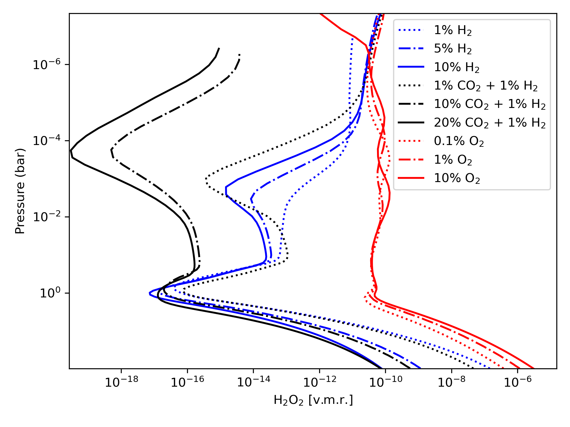
Appendix D Secondary analyses

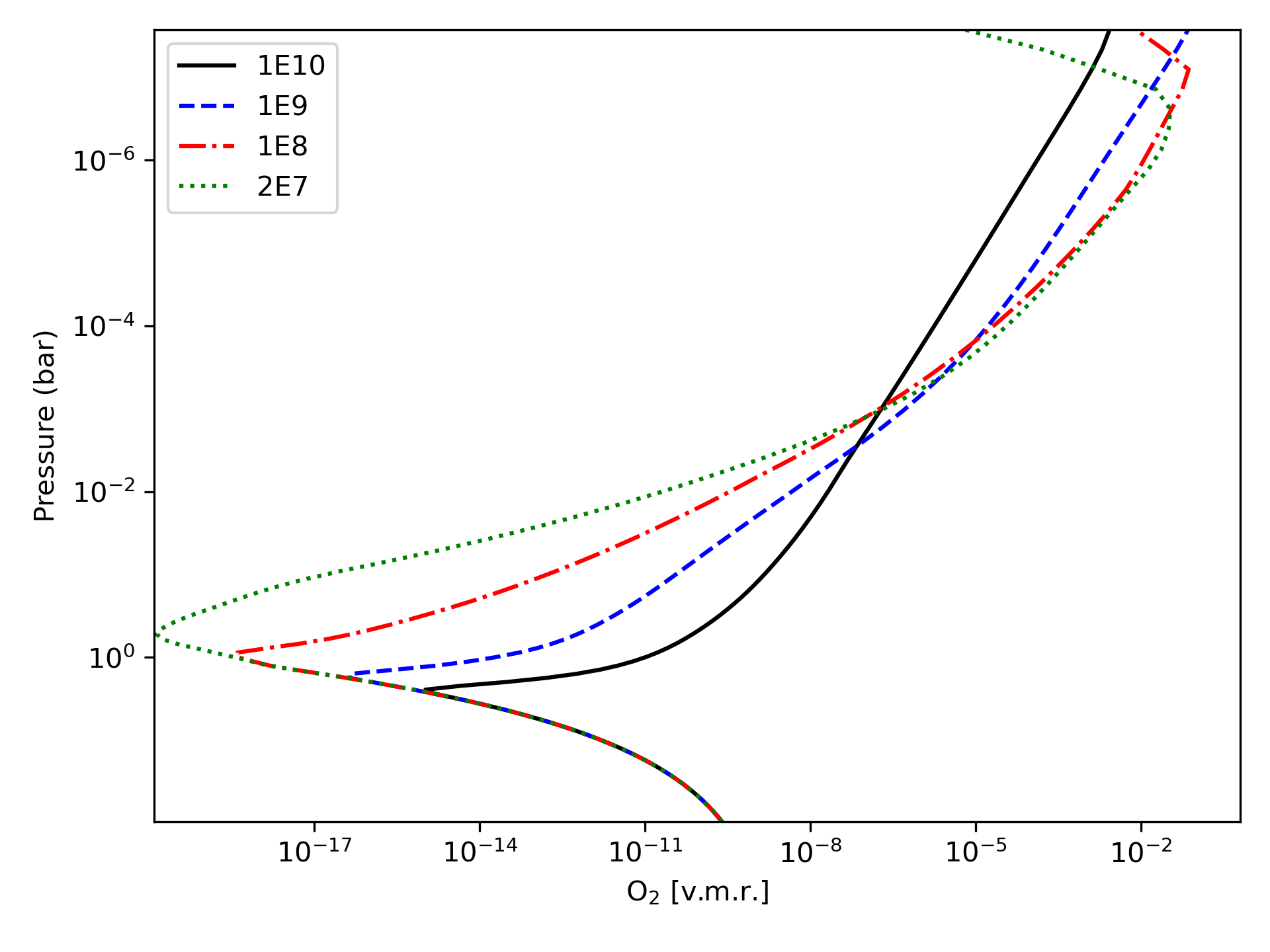

References
- Aguichine et al. (2021) Aguichine, A., Mousis, O., Deleuil, M., & Marcq, E. 2021, Mass-radius relationships for irradiated ocean planets. https://arxiv.org/abs/2105.01102
- Ali-Dib et al. (2014) Ali-Dib, M., Mousis, O., Petit, J.-M., & Lunine, J. I. 2014, The Astrophysical Journal, 793, 9
- Ardaseva et al. (2017) Ardaseva, A., Rimmer, P. B., Waldmann, I., et al. 2017, Monthly Notices of the Royal Astronomical Society, 470, 187
- Armstrong et al. (2020) Armstrong, D. J., Lopez, T. A., Adibekyan, V., et al. 2020, Nature, 583, 39
- Arney et al. (2017) Arney, G. N., Meadows, V. S., Domagal-Goldman, S. D., et al. 2017, The Astrophysical Journal, 836, 49
- Atri & Mogan (2021) Atri, D., & Mogan, S. R. C. 2021, Monthly Notices of the Royal Astronomical Society: Letters, 500, L1
- Bailey & Stevenson (2019) Bailey, E., & Stevenson, D. J. 2019, AGUFM, 2019, P11A
- Bakos et al. (2004) Bakos, G., Noyes, R., Kovács, G., et al. 2004, Publications of the Astronomical Society of the Pacific, 116, 266
- Banks & Kockarts (1973) Banks, P. M., & Kockarts, G. 1973, Aeronomy (Academic Press)
- Baraffe et al. (2015) Baraffe, I., Homeier, D., Allard, F., & Chabrier, G. 2015, Astronomy & Astrophysics, 577, A42
- Barclay et al. (2018) Barclay, T., Pepper, J., & Quintana, E. V. 2018, The Astrophysical Journal Supplement Series, 239, 2
- Barclay et al. (2013) Barclay, T., Burke, C. J., Howell, S. B., et al. 2013, The Astrophysical Journal, 768, 101
- Barnes et al. (2020) Barnes, R., Luger, R., Deitrick, R., et al. 2020, Publications of the Astronomical Society of the Pacific, 132, 024502
- Batalha et al. (2017a) Batalha, N. E., Kempton, E. M.-R., & Mbarek, R. 2017a, The Astrophysical Journal Letters, 836, L5
- Batalha et al. (2017b) Batalha, N. E., Mandell, A., Pontoppidan, K., et al. 2017b, Publications of the Astronomical Society of the Pacific, 129, 064501
- Batalha (2014) Batalha, N. M. 2014, Proceedings of the National Academy of Sciences, 111, 12647
- Bean et al. (2021) Bean, J. L., Raymond, S. N., & Owen, J. E. 2021, Journal of Geophysical Research: Planets, 126, e2020JE006639
- Benneke et al. (2019) Benneke, B., Knutson, H. A., Lothringer, J., et al. 2019, Nature Astronomy, 3, 813
- Bixel & Apai (2020) Bixel, A., & Apai, D. 2020, The Astrophysical Journal, 896, 131
- Bolmont et al. (2017) Bolmont, E., Selsis, F., Owen, J. E., et al. 2017, Monthly Notices of the Royal Astronomical Society, 464, 3728
- Borucki et al. (2010) Borucki, W. J., Koch, D., Basri, G., et al. 2010, Science, 327, 977
- Bouhlel et al. (2019) Bouhlel, M. A., Hwang, J. T., Bartoli, N., et al. 2019, Advances in Engineering Software, 102662, doi: https://doi.org/10.1016/j.advengsoft.2019.03.005
- Brugger et al. (2017) Brugger, B., Mousis, O., Deleuil, M., & Deschamps, F. 2017, The Astrophysical Journal, 850, 93
- Burke et al. (2015) Burke, C. J., Christiansen, J. L., Mullally, F., et al. 2015, The Astrophysical Journal, 809, 8
- Burrows & Sharp (1999) Burrows, A., & Sharp, C. 1999, The Astrophysical Journal, 512, 843
- Cavalié et al. (2017) Cavalié, T., Venot, O., Selsis, F., et al. 2017, Icarus, 291, 1
- Charnay et al. (2020) Charnay, B., Blain, D., Bézard, B., et al. 2020, arXiv preprint arXiv:2011.11553
- Chau et al. (2011) Chau, R., Hamel, S., & Nellis, W. J. 2011, Nature communications, 2, 1
- Chen & Rogers (2016) Chen, H., & Rogers, L. A. 2016, The Astrophysical Journal, 831, 180
- Chen et al. (2019) Chen, H., Wolf, E. T., Zhan, Z., & Horton, D. E. 2019, The Astrophysical Journal, 886, 16
- Chouqar et al. (2020) Chouqar, J., Benkhaldoun, Z., Jabiri, A., et al. 2020, Monthly Notices of the Royal Astronomical Society, 495, 962
- Cohen et al. (2015) Cohen, O., Ma, Y., Drake, J. J., et al. 2015, The Astrophysical Journal, 806, 41
- Cranmer (2004) Cranmer, S. R. 2004, American Journal of Physics, 72, 1397
- Cuntz & Wang (2018) Cuntz, M., & Wang, Z. 2018, Research Notes of the AAS, 2, 19, doi: 10.3847/2515-5172/aaaa67
- Dai et al. (2019) Dai, F., Masuda, K., Winn, J. N., & Zeng, L. 2019, The Astrophysical Journal, 883, 79
- Delrez et al. (2018) Delrez, L., Gillon, M., Queloz, D., et al. 2018, in Ground-based and Airborne Telescopes VII, Vol. 10700, International Society for Optics and Photonics, 107001I
- Demory et al. (2020) Demory, B. O., Pozuelos, F. J., Gomez Maqueo Chew, Y., et al. 2020, arXiv e-prints, arXiv:2009.04317. https://arxiv.org/abs/2009.04317
- Deschamps & Sotin (2001) Deschamps, F., & Sotin, C. 2001, Journal of Geophysical Research: Planets, 106, 5107
- Dodson-Robinson & Bodenheimer (2010) Dodson-Robinson, S. E., & Bodenheimer, P. 2010, Icarus, 207, 491
- Dorn et al. (2015) Dorn, C., Khan, A., Heng, K., et al. 2015, Astronomy & Astrophysics, 577, A83
- Dragomir et al. (2012) Dragomir, D., Matthews, J. M., Kuschnig, R., et al. 2012, The Astrophysical Journal, 759, 2
- Dressing & Charbonneau (2013) Dressing, C. D., & Charbonneau, D. 2013, The Astrophysical Journal, 767, 95
- Driscoll & Bercovici (2013) Driscoll, P., & Bercovici, D. 2013, Icarus, 226, 1447
- Ercolano & Clarke (2010) Ercolano, B., & Clarke, C. 2010, Monthly Notices of the Royal Astronomical Society, 402, 2735
- Erkaev et al. (2007) Erkaev, N., Kulikov, Y. N., Lammer, H., et al. 2007, Astronomy & Astrophysics, 472, 329
- Estrela et al. (2020) Estrela, R., Swain, M. R., Gupta, A., Sotin, C., & Valio, A. 2020, The Astrophysical Journal, 898, 104
- Fauchez et al. (2019) Fauchez, T. J., Turbet, M., Villanueva, G. L., et al. 2019, ApJ, 887, 194, doi: 10.3847/1538-4357/ab5862
- Fauchez et al. (2020) Fauchez, T. J., Villanueva, G. L., Schwieterman, E. W., et al. 2020, Nature Astronomy, 4, 372
- Fortney et al. (2021) Fortney, J. J., Dawson, R. I., & Komacek, T. D. 2021, Journal of Geophysical Research: Planets, 126, e2020JE006629, doi: https://doi.org/10.1029/2020JE006629
- Fortney et al. (2007) Fortney, J. J., Marley, M. S., & Barnes, J. W. 2007, The Astrophysical Journal, 659, 1661
- France et al. (2016) France, K., Loyd, R. P., Youngblood, A., et al. 2016, The Astrophysical Journal, 820, 89
- France et al. (2020) France, K., Duvvuri, G., Egan, H., et al. 2020, The Astronomical Journal, 160, 237
- Fu et al. (2009) Fu, R., O’Connell, R. J., & Sasselov, D. D. 2009, The Astrophysical Journal, 708, 1326
- Fulton & Petigura (2018) Fulton, B. J., & Petigura, E. A. 2018, The Astronomical Journal, 156, 264
- Fulton et al. (2017) Fulton, B. J., Petigura, E. A., Howard, A. W., et al. 2017, The Astronomical Journal, 154, 109
- Gaia Collaboration et al. (2018) Gaia Collaboration, Brown, A. G. A., Vallenari, A., et al. 2018, A&A, 616, A1, doi: 10.1051/0004-6361/201833051
- Gando et al. (2011) Gando, A., Dwyer, D., McKeown, R., Zhang, C., & the KamLAND Collaboration. 2011, Nature Geoscience, 4, 647
- Gao et al. (2018) Gao, P., Marley, M. S., & Ackerman, A. S. 2018, The Astrophysical Journal, 855, 86
- Gao et al. (2017) Gao, P., Marley, M. S., Zahnle, K., Robinson, T. D., & Lewis, N. K. 2017, The Astronomical Journal, 153, 139
- Gillon et al. (2017) Gillon, M., Triaud, A. H., Demory, B.-O., et al. 2017, Nature, 542, 456
- Ginzburg et al. (2018) Ginzburg, S., Schlichting, H. E., & Sari, R. 2018, Monthly Notices of the Royal Astronomical Society, 476, 759
- Greene et al. (2016) Greene, T. P., Line, M. R., Montero, C., et al. 2016, The Astrophysical Journal, 817, 17
- Gronoff et al. (2020) Gronoff, G., Arras, P., Baraka, S., et al. 2020, Journal of Geophysical Research: Space Physics, e2019JA027639
- Gupta & Schlichting (2020) Gupta, A., & Schlichting, H. E. 2020, Monthly Notices of the Royal Astronomical Society, 493, 792
- Haar et al. (1984) Haar, L., Gallagher, J., & Kell, G. 1984, NBS/NRC Steam Tables: Thermodynamic and Transport Properties and Computer Programs for Vapor and Liquid States of Water in SI Units (Hemisphere Publishing Corporation, Washington)
- Hamano et al. (2013) Hamano, K., Abe, Y., & Genda, H. 2013, Nature, 497, 607
- Hardegree-Ullman et al. (2019) Hardegree-Ullman, K. K., Cushing, M. C., Muirhead, P. S., & Christiansen, J. L. 2019, The Astronomical Journal, 158, 75
- He et al. (2018) He, C., Hörst, S. M., Lewis, N. K., et al. 2018, The Astronomical Journal, 156, 38
- He et al. (2020a) —. 2020a, The Planetary Science Journal, 1, 51
- He et al. (2020b) —. 2020b, Nature Astronomy, 1
- Helled et al. (2010) Helled, R., Anderson, J. D., Podolak, M., & Schubert, G. 2010, The Astrophysical Journal, 726, 15
- Hellier et al. (2012) Hellier, C., Anderson, D., Collier Cameron, A., et al. 2012, Monthly Notices of the Royal Astronomical Society, 426, 739
- Hidalgo et al. (2018) Hidalgo, S. L., Pietrinferni, A., Cassisi, S., et al. 2018, The Astrophysical Journal, 856, 125
- Hörst et al. (2018) Hörst, S. M., He, C., Ugelow, M. S., et al. 2018, The Astrophysical Journal, 858, 119
- Hu & Seager (2014) Hu, R., & Seager, S. 2014, The Astrophysical Journal, 784, 63
- Hubbard (1981) Hubbard, W. B. 1981, Science, 214, 145
- Hunten (1973) Hunten, D. M. 1973, Journal of Atmospheric Sciences, 30, 1481
- Hunten et al. (1987) Hunten, D. M., Pepin, R. O., & Walker, J. C. 1987, Icarus, 69, 532
- Jehin et al. (2011) Jehin, E., Gillon, M., Queloz, D., et al. 2011, Msngr, 145, 2
- Jin et al. (2003) Jin, R., Chen, W., & Sudjianto, A. 2003, in International Design Engineering Technical Conferences and Computers and Information in Engineering Conference, Vol. 37009, 545–554
- Johnstone et al. (2015a) Johnstone, C., Güdel, M., Brott, I., & Lüftinger, T. 2015a, Astronomy & Astrophysics, 577, A28
- Johnstone et al. (2015b) Johnstone, C., Güdel, M., Stökl, A., et al. 2015b, The Astrophysical Journal Letters, 815, L12
- Johnstone (2020) Johnstone, C. P. 2020, The Astrophysical Journal, 890, 79
- Kane et al. (2013) Kane, S. R., Barclay, T., & Gelino, D. M. 2013, The Astrophysical Journal Letters, 770, L20
- Kane et al. (2018) Kane, S. R., Ceja, A. Y., Way, M. J., & Quintana, E. V. 2018, The Astrophysical Journal, 869, 46
- Kane et al. (2020) Kane, S. R., Roettenbacher, R. M., Unterborn, C. T., Foley, B. J., & Hill, M. L. 2020, A Volatile-Poor Formation of LHS 3844b based on its Lack of Significant Atmosphere. https://arxiv.org/abs/2007.14493
- Kasting (1988) Kasting, J. F. 1988, Icarus, 74, 472
- Kasting & Pollack (1983) Kasting, J. F., & Pollack, J. B. 1983, Icarus, 53, 479
- Kasting et al. (1993) Kasting, J. F., Whitmire, D. P., & Reynolds, R. T. 1993, Icarus, 101, 108, doi: 10.1006/icar.1993.1010
- Katyal et al. (2019) Katyal, N., Nikolaou, A., Godolt, M., et al. 2019, The Astrophysical Journal, 875, 31
- Kawabata et al. (1980) Kawabata, K., Coffeen, D., Hansen, J., et al. 1980, Journal of Geophysical Research: Space Physics, 85, 8129
- Kawashima & Rugheimer (2019) Kawashima, Y., & Rugheimer, S. 2019, The Astronomical Journal, 157, 213
- Kempton et al. (2017) Kempton, E. M.-R., Bean, J. L., & Parmentier, V. 2017, The Astrophysical Journal Letters, 845, L20
- King & Wheatley (2020) King, G. W., & Wheatley, P. J. 2020, arXiv e-prints, arXiv:2007.13731. https://arxiv.org/abs/2007.13731
- Kislyakova et al. (2013) Kislyakova, K. G., Lammer, H., Holmström, M., et al. 2013, Astrobiology, 13, 1030
- Kite & Barnett (2020) Kite, E. S., & Barnett, M. N. 2020, Proceedings of the National Academy of Sciences, 117, 18264
- Kite et al. (2020) Kite, E. S., Fegley Jr, B., Schaefer, L., & Ford, E. B. 2020, The Astrophysical Journal, 891, 111
- Kite et al. (2009) Kite, E. S., Manga, M., & Gaidos, E. 2009, The Astrophysical Journal, 700, 1732
- Kite & Schaefer (2021) Kite, E. S., & Schaefer, L. 2021, Water on Hot Rocky Exoplanets. https://arxiv.org/abs/2103.07753
- Knudson et al. (2012) Knudson, M. D., Desjarlais, M. P., Lemke, R., et al. 2012, Physical Review Letters, 108, 091102
- Kopparapu et al. (2021) Kopparapu, R., Arney, G., Haqq-Misra, J., Lustig-Yaeger, J., & Villanueva, G. 2021, The Astrophysical Journal, 908, 164
- Kopparapu et al. (2014) Kopparapu, R. K., Ramirez, R. M., SchottelKotte, J., et al. 2014, ApJ, 787, L29, doi: 10.1088/2041-8205/787/2/L29
- Kopparapu et al. (2013) Kopparapu, R. K., Ramirez, R., Kasting, J. F., et al. 2013, ApJ, 765, 131, doi: 10.1088/0004-637X/765/2/131
- Korolev & Mazin (2003) Korolev, A. V., & Mazin, I. P. 2003, Journal of the atmospheric sciences, 60, 2957
- Koskinen et al. (2007) Koskinen, T. T., Aylward, A. D., & Miller, S. 2007, Nature, 450, 845
- Koskinen et al. (2014) Koskinen, T. T., Lavvas, P., Harris, M. J., & Yelle, R. V. 2014, Philosophical Transactions of the Royal Society A: Mathematical, Physical and Engineering Sciences, 372, 20130089
- Kral et al. (2020) Kral, Q., Davoult, J., & Charnay, B. 2020, Nature Astronomy, 4, 769
- Krämer et al. (2009) Krämer, M., Schiller, C., Afchine, A., et al. 2009, Atmospheric Chemistry and Physics, 9, 3505
- Krasnopolsky & Pollack (1994) Krasnopolsky, V., & Pollack, J. 1994, Icarus, 109, 58
- Kreidberg et al. (2019) Kreidberg, L., Koll, D. D., Morley, C., et al. 2019, Nature, 573, 87
- Kuramoto et al. (2013) Kuramoto, K., Umemoto, T., & Ishiwatari, M. 2013, Earth and Planetary Science Letters, 375, 312
- Kutner (2003) Kutner, M. L. 2003, Astronomy: A physical perspective (Cambridge University Press)
- Lavvas et al. (2019) Lavvas, P., Koskinen, T., Steinrueck, M. E., Muñoz, A. G., & Showman, A. P. 2019, The Astrophysical Journal, 878, 118
- Lee & Chiang (2016) Lee, E. J., & Chiang, E. 2016, The Astrophysical Journal, 817, 90
- Lee et al. (2014) Lee, E. J., Chiang, E., & Ormel, C. W. 2014, The Astrophysical Journal, 797, 95
- Lehmer et al. (2020) Lehmer, O. R., Catling, D. C., & Krissansen-Totton, J. 2020, Nature communications, 11, 1
- Lincowski et al. (2018) Lincowski, A. P., Meadows, V. S., Crisp, D., et al. 2018, The Astrophysical Journal, 867, 76
- Lissauer (2007) Lissauer, J. J. 2007, The Astrophysical Journal Letters, 660, L149
- Liu et al. (2019) Liu, B., Lambrechts, M., Johansen, A., & Liu, F. 2019, Astronomy & Astrophysics, 632, A7
- Lodders & Fegley Jr (1994) Lodders, K., & Fegley Jr, B. 1994, Icarus, 112, 368
- Lodders & Fegley Jr (2002) —. 2002, Icarus, 155, 393
- Lopez (2017) Lopez, E. D. 2017, Monthly Notices of the Royal Astronomical Society, 472, 245
- Lopez & Fortney (2014) Lopez, E. D., & Fortney, J. J. 2014, The Astrophysical Journal, 792, 1
- Loyd et al. (2020) Loyd, R. P., Shkolnik, E. L., Schneider, A. C., et al. 2020, The Astrophysical Journal, 890, 23
- Loyd et al. (2016) Loyd, R. P., France, K., Youngblood, A., et al. 2016, The Astrophysical Journal, 824, 102
- Luger & Barnes (2015) Luger, R., & Barnes, R. 2015, Astrobiology, 15, 119
- Luger et al. (2015) Luger, R., Barnes, R., Lopez, E., et al. 2015, Astrobiology, 15, 57
- Lustig-Yaeger et al. (2019a) Lustig-Yaeger, J., Meadows, V. S., & Lincowski, A. P. 2019a, The Astronomical Journal, 158, 27
- Lustig-Yaeger et al. (2019b) —. 2019b, The Astrophysical Journal Letters, 887, L11
- Madhusudhan et al. (2016) Madhusudhan, N., Agúndez, M., Moses, J. I., & Hu, Y. 2016, Space science reviews, 205, 285
- Mahadevan et al. (2012) Mahadevan, S., Ramsey, L., Bender, C., et al. 2012, in Ground-based and Airborne Instrumentation for Astronomy IV, Vol. 8446, International Society for Optics and Photonics, 84461S
- Mahadevan et al. (2014) Mahadevan, S., Ramsey, L. W., Terrien, R., et al. 2014, in Ground-based and Airborne Instrumentation for Astronomy V, Vol. 9147, International Society for Optics and Photonics, 91471G
- Marcus et al. (2010) Marcus, R. A., Sasselov, D., Hernquist, L., & Stewart, S. T. 2010, The Astrophysical Journal Letters, 712, L73
- Meadows et al. (2018) Meadows, V. S., Reinhard, C. T., Arney, G. N., et al. 2018, Astrobiology, 18, 630
- Meyer et al. (1983) Meyer, C. A., McClintock, R. B., Silvestri, G. J., & Spencer, R. C. 1983, ASME Steam Tables: Thermodynamic and Transport Properties of Steam (American Society of Mechanical Engineers, Fifth Edition)
- Mikal-Evans et al. (2020) Mikal-Evans, T., Crossfield, I. J., Benneke, B., et al. 2020, The Astronomical Journal, 161, 18
- Millot et al. (2018) Millot, M., Hamel, S., Rygg, J. R., et al. 2018, Nature Physics, 14, 297
- Misener & Schlichting (2021) Misener, W., & Schlichting, H. E. 2021, arXiv preprint arXiv:2103.09212
- Misra et al. (2014) Misra, A., Meadows, V., Claire, M., & Crisp, D. 2014, Astrobiology, 14, 67
- Moore & Cowan (2020) Moore, K., & Cowan, N. B. 2020, arXiv preprint arXiv:2006.08514
- Moran et al. (2018) Moran, S. E., Hörst, S. M., Batalha, N. E., Lewis, N. K., & Wakeford, H. R. 2018, The Astronomical Journal, 156, 252
- Moran et al. (2020) Moran, S. E., Hörst, S. M., Vuitton, V., et al. 2020, The Planetary Science Journal, 1, 17
- Mordasini et al. (2009) Mordasini, C., Alibert, Y., & Benz, W. 2009, Astronomy & Astrophysics, 501, 1139
- Moses et al. (2020) Moses, J., Cavalié, T., Fletcher, L., & Roman, M. 2020, Philosophical Transactions of the Royal Society A, 378, 20190477
- Mousis et al. (2020a) Mousis, O., Aguichine, A., Atkinson, D. H., et al. 2020a, Space Science Reviews, 216, 1
- Mousis et al. (2020b) Mousis, O., Deleuil, M., Aguichine, A., et al. 2020b, arXiv preprint arXiv:2002.05243
- Mueller-Wodarg et al. (2008) Mueller-Wodarg, I., Strobel, D., Moses, J., et al. 2008, Space science reviews, 139, 191
- Murray-Clay et al. (2009) Murray-Clay, R. A., Chiang, E. I., & Murray, N. 2009, The Astrophysical Journal, 693, 23
- Nettelmann et al. (2016) Nettelmann, N., Wang, K., Fortney, J. J., et al. 2016, Icarus, 275, 107
- Nikolaou et al. (2019) Nikolaou, A., Katyal, N., Tosi, N., et al. 2019, The Astrophysical Journal, 875, 11
- Noack et al. (2016) Noack, L., Höning, D., Rivoldini, A., et al. 2016, Icarus, 277, 215
- Owen & Alvarez (2016) Owen, J. E., & Alvarez, M. A. 2016, The Astrophysical Journal, 816, 34
- Owen & Campos Estrada (2020) Owen, J. E., & Campos Estrada, B. 2020, Monthly Notices of the Royal Astronomical Society, 491, 5287
- Owen & Jackson (2012) Owen, J. E., & Jackson, A. P. 2012, Monthly Notices of the Royal Astronomical Society, 425, 2931
- Owen & Wu (2013) Owen, J. E., & Wu, Y. 2013, The Astrophysical Journal, 775, 105
- Owen & Wu (2016) —. 2016, The Astrophysical Journal, 817, 107
- Owen & Wu (2017) —. 2017, The Astrophysical Journal, 847, 29
- Peacock et al. (2020) Peacock, S., Barman, T., Shkolnik, E. L., et al. 2020, The Astrophysical Journal, 895, 5
- Pearl & Conrath (1991) Pearl, J., & Conrath, B. 1991, Journal of Geophysical Research: Space Physics, 96, 18921
- Pidhorodetska et al. (2021) Pidhorodetska, D., Moran, S. E., Schwieterman, E. W., et al. 2021, L 98-59: a Benchmark System of Small Planets for Future Atmospheric Characterization. https://arxiv.org/abs/2106.00685
- Piette & Madhusudhan (2020) Piette, A. A., & Madhusudhan, N. 2020, arXiv preprint arXiv:2009.11290
- Pollacco et al. (2006) Pollacco, D. L., Skillen, I., Cameron, A. C., et al. 2006, Publications of the Astronomical Society of the Pacific, 118, 1407
- Poppenhaeger et al. (2020) Poppenhaeger, K., Ketzer, L., & Mallonn, M. 2020, Monthly Notices of the Royal Astronomical Society
- Rafikov (2006) Rafikov, R. R. 2006, The Astrophysical Journal, 648, 666
- Rafikov (2011) —. 2011, The Astrophysical Journal, 727, 86
- Ramirez & Kaltenegger (2014) Ramirez, R. M., & Kaltenegger, L. 2014, The Astrophysical Journal Letters, 797, L25
- Ranjan et al. (2020) Ranjan, S., Schwieterman, E. W., Harman, C., et al. 2020, arXiv preprint arXiv:2004.04185
- Redmer et al. (2011) Redmer, R., Mattsson, T. R., Nettelmann, N., & French, M. 2011, Icarus, 211, 798
- Reed et al. (2020) Reed, N. W., Browne, E. C., & Tolbert, M. A. 2020, ACS Earth and Space Chemistry, 4, 897
- Ricker et al. (2014) Ricker, G. R., Winn, J. N., Vanderspek, R., et al. 2014, Journal of Astronomical Telescopes, Instruments, and Systems, 1, 014003
- Rogers & Seager (2010) Rogers, L., & Seager, S. 2010, The Astrophysical Journal, 712, 974
- Rogers (2015) Rogers, L. A. 2015, The Astrophysical Journal, 801, 41
- Rugheimer & Kaltenegger (2018) Rugheimer, S., & Kaltenegger, L. 2018, The Astrophysical Journal, 854, 19
- Rugheimer et al. (2013) Rugheimer, S., Kaltenegger, L., Zsom, A., Segura, A., & Sasselov, D. 2013, Astrobiology, 13, 251
- Rushby et al. (2013) Rushby, A. J., Claire, M. W., Osborn, H., & Watson, A. J. 2013, Astrobiology, 13, 833
- Sanz-Forcada et al. (2011) Sanz-Forcada, J., Micela, G., Ribas, I., et al. 2011, Astronomy & Astrophysics, 532, A6
- Schaefer & Fegley Jr (2010) Schaefer, L., & Fegley Jr, B. 2010, Icarus, 208, 438
- Schaefer & Fegley Jr (2011) —. 2011, The Astrophysical Journal, 729, 6
- Schaefer et al. (2016) Schaefer, L., Wordsworth, R. D., Berta-Thompson, Z., & Sasselov, D. 2016, The Astrophysical Journal, 829, 63
- Schubert & Soderlund (2011) Schubert, G., & Soderlund, K. M. 2011, Physics of the Earth and Planetary Interiors, 187, 92
- Schwieterman et al. (2019) Schwieterman, E. W., Reinhard, C. T., Olson, S. L., et al. 2019, The Astrophysical Journal, 874, 9
- Seager et al. (2007) Seager, S., Kuchner, M., Hier-Majumder, C., & Militzer, B. 2007, The Astrophysical Journal, 669, 1279
- Segura et al. (2005) Segura, A., Kasting, J. F., Meadows, V., et al. 2005, Astrobiology, 5, 706
- Segura et al. (2003) Segura, A., Krelove, K., Kasting, J. F., et al. 2003, Astrobiology, 3, 689
- Selsis et al. (2007) Selsis, F., Kasting, J. F., Levrard, B., et al. 2007, Astronomy & Astrophysics, 476, 1373
- Soubiran & Militzer (2015) Soubiran, F., & Militzer, B. 2015, The Astrophysical Journal, 806, 228
- Stefansson et al. (2020) Stefansson, G., Kopparapu, R., Lin, A., et al. 2020, arXiv e-prints, arXiv:2006.11180. https://arxiv.org/abs/2006.11180
- Stelzer et al. (2013) Stelzer, B., Marino, A., Micela, G., López-Santiago, J., & Liefke, C. 2013, Monthly Notices of the Royal Astronomical Society, 431, 2063
- Tian & Stanley (2013) Tian, B. Y., & Stanley, S. 2013, The Astrophysical Journal, 768, 156
- Tian (2009) Tian, F. 2009, The Astrophysical Journal, 703, 905
- Tian (2015) —. 2015, Earth and Planetary Science Letters, 432, 126
- Tilley et al. (2019) Tilley, M. A., Segura, A., Meadows, V., Hawley, S., & Davenport, J. 2019, Astrobiology, 19, 64
- Toon et al. (1989) Toon, O. B., McKay, C. P., Ackerman, T. P., & Santhanam, K. 1989, J. Geophys. Res., 94, 16287, doi: 10.1029/JD094iD13p16287
- Tsai et al. (2017) Tsai, S.-M., Lyons, J. R., Grosheintz, L., et al. 2017, The Astrophysical Journal Supplement Series, 228, 20
- Tsang et al. (2010) Tsang, C. C., Wilson, C. F., Barstow, J. K., et al. 2010, Geophysical research letters, 37
- Turbet et al. (2020) Turbet, M., Bolmont, E., Ehrenreich, D., et al. 2020, Astronomy & Astrophysics, 638, A41
- Twicken et al. (2016) Twicken, J. D., Jenkins, J. M., Seader, S. E., et al. 2016, The Astronomical Journal, 152, 158
- Unterborn et al. (2016) Unterborn, C. T., Dismukes, E. E., & Panero, W. R. 2016, The Astrophysical Journal, 819, 32
- Valencia et al. (2013) Valencia, D., Guillot, T., Parmentier, V., & Freedman, R. S. 2013, The Astrophysical Journal, 775, 10
- Venot et al. (2014) Venot, O., Agúndez, M., Selsis, F., Tessenyi, M., & Iro, N. 2014, Astronomy & Astrophysics, 562, A51
- Venturini & Helled (2017) Venturini, J., & Helled, R. 2017, The Astrophysical Journal, 848, 95
- Villanueva et al. (2018) Villanueva, G. L., Smith, M. D., Protopapa, S., Faggi, S., & Mandell, A. M. 2018, J. Quant. Spec. Radiat. Transf., 217, 86, doi: 10.1016/j.jqsrt.2018.05.023
- Villanueva et al. (2018) Villanueva, G. L., Smith, M. D., Protopapa, S., Faggi, S., & Mandell, A. M. 2018, Journal of Quantitative Spectroscopy and Radiative Transfer, 217, 86
- Visscher & Moses (2011) Visscher, C., & Moses, J. I. 2011, The Astrophysical Journal, 738, 72
- Visscher et al. (2010) Visscher, C., Moses, J. I., & Saslow, S. A. 2010, Icarus, 209, 602
- Vuitton et al. (2021) Vuitton, V., Moran, S. E., He, C., et al. 2021, The Planetary Science Journal, 2, 2
- Walker (1975) Walker, J. C. 1975, Journal of the Atmospheric Sciences, 32, 1248
- Wallace & Hobbs (2006) Wallace, J. M., & Hobbs, P. V. 2006, Atmospheric science: an introductory survey, Vol. 92 (Elsevier)
- Wang et al. (2016) Wang, Y., Tian, F., Li, T., & Hu, Y. 2016, Icarus, 266, 15
- Way & Del Genio (2020) Way, M., & Del Genio, A. D. 2020, Journal of Geophysical Research: Planets, 125, e2019JE006276
- Way et al. (2016) Way, M. J., Del Genio, A. D., Kiang, N. Y., et al. 2016, Geophysical research letters, 43, 8376
- Weiss et al. (2018) Weiss, L. M., Marcy, G. W., Petigura, E. A., et al. 2018, The Astronomical Journal, 155, 48
- Welbanks & Madhusudhan (2019) Welbanks, L., & Madhusudhan, N. 2019, The Astronomical Journal, 157, 206
- Wilson & Militzer (2011) Wilson, H. F., & Militzer, B. 2011, The Astrophysical Journal, 745, 54
- Wolfgang & Lopez (2015) Wolfgang, A., & Lopez, E. 2015, The Astrophysical Journal, 806, 183
- Youngblood et al. (2016) Youngblood, A., France, K., Loyd, R. P., et al. 2016, The Astrophysical Journal, 824, 101
- Yu et al. (2021) Yu, X., Moses, J. I., Fortney, J. J., & Zhang, X. 2021, How to identify exoplanet surfaces using atmospheric trace species in hydrogen-dominated atmospheres. https://arxiv.org/abs/2104.09843
- Yung et al. (2009) Yung, Y. L., Liang, M., Jiang, X., et al. 2009, Journal of Geophysical Research: Planets, 114
- Zahnle et al. (2009) Zahnle, K., Marley, M., Freedman, R. S., Lodders, K., & Fortney, J. 2009, The Astrophysical Journal Letters, 701, L20
- Zahnle et al. (2016) Zahnle, K., Marley, M. S., Morley, C. V., & Moses, J. I. 2016, The Astrophysical Journal, 824, 137
- Zahnle & Kasting (1986) Zahnle, K. J., & Kasting, J. F. 1986, Icarus, 68, 462
- Zahnle et al. (1988) Zahnle, K. J., Kasting, J. F., & Pollack, J. B. 1988, Icarus, 74, 62
- Zeng et al. (2019) Zeng, L., Jacobsen, S. B., Sasselov, D. D., et al. 2019, Proceedings of the National Academy of Sciences, 116, 9723