Sign freedom of non-Abelian topological charges in phononic and photonic topological insulatorsPreprint: APS/123-QED
Abstract
The topological nature of nodal lines in a three-band system can be described by non-Abelian topological charges called quaternion numbers. Due to the gauge freedom of the eigenstates, the sign of the non-Abelian topological charges can be flipped by performing the gauge transformation, i.e., choosing a different basis of eigenstates. However, the sign flipping has not been explicitly shown in realistic systems such as phononic and photonic topological insulators. Here, we elaborate the sign freedom by visualizing the numerically calculated topological charges in phononic and photonic topological insulators. In doing so, we employ a common reference point method for multiple nodal lines to confirm that the sign flipping does not cause any issue in building the quaternion group.
I Introduction
Multiple nodal lines in the momentum space can be interpreted by non-Abelian band topology Wu et al. 2019. In particular, topological charges (invariants) of nodal lines in a three-band system can be expressed by the quaternion group Wu et al. 2019. Recently, a lot of studies on the nodal lines Lenggenhager et al. 2021; Bouhon et al. 2020a; Xia et al. 2019; Ahn et al. 2018; Kim et al. 2020 have been reported, including nodal rings Deng et al. 2019; Gao et al. 2018, nodal chains Bzdušek et al. 2016; Yan et al. 2018; Chang et al. 2017; Yan et al. 2017; Belopolski et al. 2019, nodal links Chang et al. 2017; Yan et al. 2017; Belopolski et al. 2019; Yang et al. 2020a; He et al. 2020a; Xie et al. 2019; Lee et al. 2020; Yang et al. 2020b, and nodal knots Lee et al. 2020; Yang et al. 2020b; Bi et al. 2017. Theoretical and experimental efforts have been made to demonstrate the quaternion topological charges in such nodal line systems Park et al. 2021; Yang et al. 2020a; Wang et al. 2021; Yang et al. 2021; Guo et al. 2021. Hence, the field of research on the non-Abelian topological nodal lines is rapidly expanding along with the study on Dirac Slobozhanyuk et al. 2017; Lu et al. 2016; Jin et al. 2017; Liu et al. 2020; Abbaszadeh et al. 2017; Brendel et al. 2017; Wang et al. 2015; Wen et al. 2019 and Weyl points Lu et al. 2013; Lu et al. 2015; Park and Lee 2020; He et al. 2018; Peri et al. 2019; He et al. 2020b; Jia et al. 2019; Yang et al. 2018; Yang et al. 2019; Soluyanov et al. 2015.
Although the gauge-dependent property of the non-Abelian charge has been already discussed Wu et al. 2019; Bouhon et al. 2019; Bouhon et al. 2020b; Tiwari and Bzdušek 2020; Guo et al. 2021; Jiang et al. 2021; Peng et al. 2021, such a property has not been explained by visualizing the eigenstates. In any eigenvalue problems, if is an eigenstate of a system, () is also an eigenstate of the system, and these two are regarded as the equivalent states (gauge freedom). Even if we assume only a real number , i.e., or , the eigenstates of the system can be expressed either by or . This gauge freedom may generate any signs of the topological invariants in the nodal line system. Notably, this property does not contradict the argument of the non-Abelian band topology in a three-band system and it is important to fix the basis of eigenstates as pointed out in Ref. Wu et al. 2019.
In this paper, we elucidate the gauge-dependent sign freedom of the non-Abelian topological charges by visualizing the topological charges in phononic and photonic topological insulators. First, we exemplify such a property with phononic and photonic systems. Then, the reference point method which can be thought as fixing the basis of Hilbert space Wu et al. 2019; Tiwari and Bzdušek 2020 is adopted to our topological insulators. Finally, we discuss the consistency of the topological charges’ non-Abelian relations and the considerations of using this method in phononic and photonic topological insulators regarding the non-Abelian topological charges.
II Gauge-dependent property of topological charges
Obtaining the quaternion charge of a nodal line starts by calculating eigenstates along the closed loop that encloses the nodal line. We denote the starting point of the closed loop’s winding as . Once the signs of the eigenstates at are determined, their signs at subsequent points on the loop are assigned. Finally, the topological charges are calculated by analyzing the rotation behaviors of the eigenstates. Due to the sign freedom of the eigenstates at , the topological charge also has the sign freedom Wu et al. 2019; Bouhon et al. 2019; Bouhon et al. 2020b; Tiwari and Bzdušek 2020; Guo et al. 2021; Jiang et al. 2021; Peng et al. 2021. In this section, we discuss the examples that show the sign freedom of the quaternion charges originating from the sign freedom of eigenstates at .


II.1 Hamiltonian
We consider phononic waves in an orthotropic elastic material Beer et al. 2012 whose constitutive equation is given by Hooke’s law . Here, and () are the Cauchy strain and stress tensors, respectively. is a compliance matrix, which is a function of Young’s moduli, shear moduli and Poisson’s ratios: . Its inverse is the stiffness matrix , i.e., , thereby the consitutive equation becomes which is analogous to the one-dimensional Hooke’s law .
By using the density , Young’s moduli , shear moduli , Poisson’s ratios , and restoring forces () listed in Table 1 in Appendix A, the eigenvalue problem for this elastic wave system is expressed as
| (1) |
where () is the three-component displacement eigenvector satisfying the orthonormal condition , and is the angular frequency as an eigenfrequency [the detailed derivation of Eq. (1) is written in Appendix A]. Here, the superscript is the band number, and is a point in the momentum space.
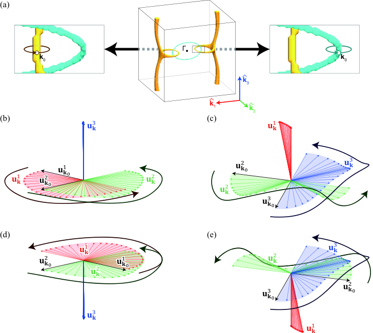
For the nodal link shown in Fig. 1(a) in this phononic system, we choose two closed loops [the arrowed loops in Fig. 1(a)] that enclose each nodal ring [the orange and cyan colored shapes Fig. 1(a), respectively]. We calculate the orthonormal eigenvectors along the closed loops Park et al. 2021. We gather all the eigenstates at the origin, and their behaviors are shown in Fig. 1(b), (c), respectively. We may regard the topological charge for Fig. 1(b) as the quaternion number because and rotate by around fixed Wu et al. 2019; Park et al. 2021; Yang et al. 2020a. Likewise, and rotate by around fixed in Fig. 1(c), and thereby its topological charge is the quaternion number Wu et al. 2019; Park et al. 2021; Yang et al. 2020a.
Meanwhile, due to the sign freedom of the eigenstates, we can choose different eigenstates at . For the orange loop in Fig. 1(a), we flip the signs of and while keeping fixed. Then, at the following points on the loop is determined by these . The resulting relation between the eigenstates exhibits -rotations of and around [see Fig. 1(d)]. Thus, the topological charge for this situation is considered as , compared to Fig. 1(b). Likewise, we apply the sign-flipping of and with fixing to the cyan loop in Fig. 1(a). It generates the -rotations of and around [see Fig. 1(e)] making its topological charge in contrast to Fig. 1(c). Therefore, the topological charges of the left and right figures of Fig. 1(a) can be any of the four sets of quaternion numbers , , , or .
II.2 Correlation vectors in photonic system
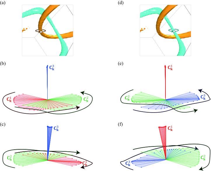
Examples of the gauge-dependent non-Abelian charge can be also visualized by the correlation vectors Park et al. 2021. For the closed loop in Fig. 2(a), we compute the orthonormal eigenstates ( for the third, fourth, and fifth bands, respectively). Then, we calculate the correlations defined by the following equation Park et al. 2021:
| (2) |
All the correlations on the closed loop are collected at the origin, as shown in Fig. 2(b). The result means its topological charge is . Now, we adjust the signs of and with fixing the sign of . The signs of at the remaining points on the closed loop are assigned by the . The resulting topological charge in Fig. 2(c) is .
Likewise, for the closed loop in Fig. 2(d), we consider two sets of . The sign of in the first set is not adjusted. For the second set, we flip the signs of and with fixing the gauge of . Thus, the topological charges of Fig. 2(e), (f) are and , respectively.

III Application of common reference point method
To fix the signs of the topological charges of our topological insulators, we fix the gauge of the eigenstates using a reference point Wu et al. 2019; Tiwari and Bzdušek 2020. We denote the common reference point as , and a line connects and of each loop, as illustrated in Fig. 3. There can be several for several closed loops while we consider only one . For example, when the topological charge on one closed loop in Fig. 3 is investigated, is calculated first. For all the remaining points on the line, is also calculated. Finally, when reaches , is determined. Then, the topological charge is calculated by the eigenstates only on the loop.
Instead of using the reference point , choosing the loops whose starting points coincide can be an alternative. However, a smaller loop generates more accurate topological charge. Thus, this alternative can be used in limited situations only, for example the nodal lines that are sufficiently close to each other.
For the phononic topological insulator, we set a common reference point as shown in Fig. 4(a), then we calculated the eigenstates of Eq. (1) along each path. The eigenstates on the closed loop of Path A are shown in Fig. 4(b), and collecting them at the origin results in [as shown in Fig. 4(c), identical to Fig. 1(b)]. Likewise, the eigenstates along Path B are plotted in Fig. 4(d) and (e) [identical to Fig. 1(c)] resulting in topological charge . The eigenstates for Path A and B should be the same at the common reference point .
The topological charge can be described by composition of the loops in Path A and B, which are the closed loops encircling both orange and cyan nodal lines. Here, the circling sequence is related to the order of and in the multiplication. If the first and second half of closed loop scan the cyan () and orange () nodal lines, respectively, the relation is written as . The signs of and are concerned with winding direction of the closed loop. Then, we can consider four relations , , , and , and their results are thus , , , and , as shown in each panel of Fig. 5, respectively. The plots in Fig. 5 are the calibrated results by Ref. Park et al. 2021. The calibration angle was set as where is the angle between and .
Note that the topological charges , , and of the double diamond photonic crystal in Ref. Park et al. 2021 were calculated using the reference point. More details will be explained in Section V.1.
IV Consistency of topological charges’ signs by the reference point method
In the following, we will elaborate that the reference point method can eliminate the chance that the non-Abelian charges are misinterpreted as Abelian. For example, let us suppose that two closed loops are in different locations [marked as Loop 1 and 2 in Fig. 6, respectively]. If we denote topological charges by these loops as and , respectively, and if we consider an additional loop [marked as Loop 3a in Fig. 6] circling along Loop 2 and 1 in sequence Park et al. 2021; Yang et al. 2020a, the Loop 3a’s topological charge is calculated by the composition of and , i.e., . We also suppose that Loop 3b scans around Loop 1 first then circles Loop 2, as shown in Fig. 6. Its topological charge is expressed as . If and satisfy , this leads to . This relation can be called ‘non-Abelian’. To write this relation, the signs of each charge should be first determined by such kind of sign convention. If there is not any sign convention, and if the topological charge of Loop 3b can be either plus or minus, it means that we can assume the sign-flipping of with fixing the other charges’ signs. Then, the above relation becomes or . Thus, such a situation could be incorrectly interpreted as ‘Abelian’. This behavior is, however, simply a result coming from the gauge freedom of the eigenstates and there is no problem in the non-Abelian nature of the non-Abelian band topology.
V Considerations of using the reference point method in phononic and photonic topological insulators
V.1 Path and degeneracies
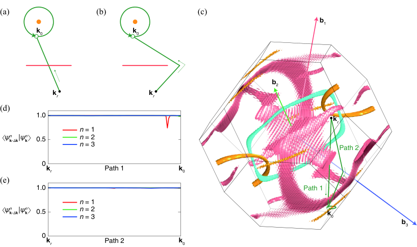
Although Fig. 3 shows the paths between and in linear forms, they do not have to be a straight line. Instead of the straight line [see Fig. 7(a)], the path sometimes should make a detour around degeneracies [see Fig. 7(b)] whichever the degeneracies are zero, one, two, or three dimensions. Suppose we investigate the topological nature by the three bands indexed as , , and . The paths should avoid the degeneracies that at least one of these three bands is concerned with, e.g., the degeneracies by the bands and or the degeneracies by the bands and . This is because the degeneracies destroy the eigenstates information at . In Fig. 7(c), Path 1 goes through the pink points (near ) while Path 2 avoids them. The pink points are degeneracies between the second and third bands ( and , respectively). () at each point on Path 1 are calculated, and only the value with shows the sharp change around the degeneracies [see Fig. 7(d)]. In contrast, their behaviors on Path 2 do not exhibit such a sharp change [see Fig. 7(e)]. In other words, the eigenstates information at cannot be delivered through the degeneracies because the degeneracies may act as the sink or source of certain topological states, like Weyl points Lu et al. 2013; Lu et al. 2015; Park and Lee 2020; He et al. 2018; Peri et al. 2019; He et al. 2020b; Jia et al. 2019; Yang et al. 2018; Yang et al. 2019; Soluyanov et al. 2015; Fruchart et al. 2018; Yang et al. 2017.
The reference point also should be fixed such that the overall distances are minimized. This is because the longer distance of may cause the loss of the Bloch states at due to the degeneracies or other unknown factors.
V.2 Gauge freedom at the reference point
Although we examined the topological charges of our topological insulators by applying the reference point method, this method does not determine the exact sign on each topological charge because the sign freedom of the eigenstates at still remains. If the eigenstates’ signs at are flipped, some quaternion charges’ signs may be flipped while the other quaternion charges’s signs do not change. For example, regarding Fig. 4 and 5, if we flip the signs of and at , the result in Fig. 4(e) may change from to while the topological charge of Fig. 4(c) is still . Fortunately, in this situation, the signs in Fig. 5 are also inverted, and therefore the non-Abelian relations between the charges survive.
VI Conclusions
In summary, we have visualized the gauge-dependent property of the non-Abelian charges Wu et al. 2019; Bouhon et al. 2019; Bouhon et al. 2020b; Tiwari and Bzdušek 2020; Guo et al. 2021; Jiang et al. 2021; Peng et al. 2021 in phononic and photonic topological insulators. We have also applied the reference point method, which is equivalent to the basis fixing Wu et al. 2019; Tiwari and Bzdušek 2020, to our topological insulators. Additionally, the consistency of non-Abelian relationship between topological charges with this method was discussed.
Based on the discussions in Section V.2, we remark the following conclusions: (i) The gauge fixing by the common reference point does not fix the quaternion charges’ signs but fix the relations between the signs. (ii) The signs of the nodal lines are adjustable by regulating the eigenstates’ signs at the reference point . (iii) The sign is not an absolute feature of the non-Abelian charge, but it is concerned with the relations between charges. In other words, the sign relation between different nodal lines is more important than the sign of absolute charges corresponding to each loop.
Acknowledgements.
The work is part-funded by the European Regional Development Fund through the Welsh Government (80762-CU145 (East)).
Appendix A Derivation of Hamiltonian for orthotropic elastic material
The constitutive equation for an orthotropic elastic material is expressed as , or
| (3) |
where and are the Cauchy strain and stress tensors, respectively (). Each component of the Cauchy strain tensor is expressed as where is the displacement vector. is the compliance tensor:
| (4) |
where is the Young’s modulus along -direction and is the shear modulus along -direction on the plane normal to -direction. is the Poisson’s ratio, the negative ratio of a transverse strain along -direction to a longitudinal strain along -direction. Because we assume an orthotropic material, the relation holds and the compliance tensor is symmetric.
| Quantities | Values |
|---|---|
| Young’s moduli (MPa) | , , |
| Shear moduli (MPa) | , |
| Poisson’s ratios (1) | , , |
| Density (kg/m3) | |
| Restoring forces (N/m3) | , , |
The wave equation for an elastic material is , where is the body force. Here, we consider the body force as the restoring force expressed as , i.e., . If the displacement vector is expressed as , substituting this into the wave equation leads Eq. (1). In Eq. (1), and are the components of the stiffness matrix as follows:
| (5) |
This orthotropic elastic material forms a nodal link when the parameters in Table 1 are used. In the given the momentum space with , , and , we calculated the eigenfrequencies . We regarded that two bands and at point are degenerated if , where m is the constant for normalization. Sets of the degeneracies formed between the first and second bands and the second and third bands are depicted as orange and cyan nodal lines, respectively, in Fig. 8(a). Band structures along and directions are also given in Fig. 8(b),(c), respectively.
References
- Wu et al. (2019) Q. Wu, A. A. Soluyanov, and T. Bzdušek, Non-abelian band topology in noninteracting metals, Science 365, 1273 (2019).
- Lenggenhager et al. (2021) P. M. Lenggenhager, X. Liu, S. S. Tsirkin, T. Neupert, and T. Bzdušek, From triple-point materials to multiband nodal links, Phys. Rev. B 103, L121101 (2021).
- Bouhon et al. (2020a) A. Bouhon, Q. Wu, R.-J. Slager, H. Weng, O. V. Yazyev, and T. Bzdušek, Non-abelian reciprocal braiding of weyl points and its manifestation in zrte, Nat. Phys. 16, 1137 (2020a).
- Xia et al. (2019) L. Xia, Q. Guo, B. Yang, J. Han, C.-X. Liu, W. Zhang, and S. Zhang, Observation of hourglass nodal lines in photonics, Phys. Rev. Lett. 122, 103903 (2019).
- Ahn et al. (2018) J. Ahn, D. Kim, Y. Kim, and B.-J. Yang, Band topology and linking structure of nodal line semimetals with monopole charges, Phys. Rev. Lett. 121, 106403 (2018).
- Kim et al. (2020) M. Kim, Z. Jacob, and J. Rho, Recent advances in 2d, 3d and higher-order topological photonics, Light Sci. Appl. 9, 130 (2020).
- Deng et al. (2019) W. Deng, J. Lu, F. Li, X. Huang, M. Yan, J. Ma, and Z. Liu, Nodal rings and drumhead surface states in phononic crystals, Nat. Commun. 10, 1769 (2019).
- Gao et al. (2018) W. Gao, B. Yang, B. Tremain, H. Liu, Q. Guo, L. Xia, A. P. Hibbins, and S. Zhang, Experimental observation of photonic nodal line degeneracies in metacrystals, Nat. Commun. 9, 950 (2018).
- Bzdušek et al. (2016) T. Bzdušek, Q. Wu, A. Rüegg, M. Sigrist, and A. A. Soluyanov, Nodal-chain metals, Nature 538, 75 (2016).
- Yan et al. (2018) Q. Yan, R. Liu, Z. Yan, B. Liu, H. Chen, Z. Wang, and L. Lu, Experimental discovery of nodal chains, Nat. Phys. 14, 461 (2018).
- Chang et al. (2017) G. Chang, S.-Y. Xu, X. Zhou, S.-M. Huang, B. Singh, B. Wang, I. Belopolski, J. Yin, S. Zhang, A. Bansil, H. Lin, and M. Z. Hasan, Topological hopf and chain link semimetal states and their application to , Phys. Rev. Lett. 119, 156401 (2017).
- Yan et al. (2017) Z. Yan, R. Bi, H. Shen, L. Lu, S.-C. Zhang, and Z. Wang, Nodal-link semimetals, Phys. Rev. B 96, 041103 (2017).
- Belopolski et al. (2019) I. Belopolski, K. Manna, D. S. Sanchez, G. Chang, B. Ernst, J. Yin, S. S. Zhang, T. Cochran, N. Shumiya, H. Zheng, B. Singh, G. Bian, D. Multer, M. Litskevich, X. Zhou, S.-M. Huang, B. Wang, T.-R. Chang, S.-Y. Xu, A. Bansil, C. Felser, H. Lin, and M. Z. Hasan, Discovery of topological weyl fermion lines and drumhead surface states in a room temperature magnet, Science 365, 1278 (2019).
- Yang et al. (2020a) E. Yang, B. Yang, O. You, H.-C. Chan, P. Mao, Q. Guo, S. Ma, L. Xia, D. Fan, Y. Xiang, and S. Zhang, Observation of non-abelian nodal links in photonics, Phys. Rev. Lett. 125, 033901 (2020a).
- He et al. (2020a) P. He, J.-H. Fu, D.-W. Zhang, and S.-L. Zhu, Double exceptional links in a three-dimensional dissipative cold atomic gas, Phys. Rev. A 102, 023308 (2020a).
- Xie et al. (2019) Y. Xie, J. Cai, J. Kim, P.-Y. Chang, and Y. Chen, Hopf-chain networks evolved from triple points, Phys. Rev. B 99, 165147 (2019).
- Lee et al. (2020) C. H. Lee, A. Sutrisno, T. Hofmann, T. Helbig, Y. Liu, Y. S. Ang, L. K. Ang, X. Zhang, M. Greiter, and R. Thomale, Imaging nodal knots in momentum space through topolectrical circuits, Nat. Commun. 11, 4385 (2020).
- Yang et al. (2020b) Z. Yang, C.-K. Chiu, C. Fang, and J. Hu, Jones polynomial and knot transitions in hermitian and non-hermitian topological semimetals, Phys. Rev. Lett. 124, 186402 (2020b).
- Bi et al. (2017) R. Bi, Z. Yan, L. Lu, and Z. Wang, Nodal-knot semimetals, Phys. Rev. B 96, 201305 (2017).
- Park et al. (2021) H. Park, S. Wong, X. Zhang, and S. S. Oh, Non-abelian charged nodal links in a dielectric photonic crystal, ACS Photonics 8, 2746 (2021).
- Wang et al. (2021) D. Wang, B. Yang, Q. Guo, R.-Y. Zhang, L. Xia, X. Su, W.-J. Chen, J. Han, S. Zhang, and C. T. Chan, Intrinsic in-plane nodal chain and generalized quaternion charge protected nodal link in photonics, Light Sci. Appl. 10, 83 (2021).
- Yang et al. (2021) B. Yang, Y. Bi, R.-X. Zhang, R.-Y. Zhang, O. You, Z. Zhu, J. Feng, H. Sun, C. T. Chan, C.-X. Liu, and S. Zhang, Momentum space toroidal moment in a photonic metamaterial, Nat. Commun. 12, 1784 (2021).
- Guo et al. (2021) Q. Guo, T. Jiang, R.-Y. Zhang, L. Zhang, Z.-Q. Zhang, B. Yang, S. Zhang, and C. T. Chan, Experimental observation of non-abelian topological charges and edge states, Nature 594, 195 (2021).
- Slobozhanyuk et al. (2017) A. Slobozhanyuk, S. H. Mousavi, X. Ni, D. Smirnova, Y. S. Kivshar, and A. B. Khanikaev, Three-dimensional all-dielectric photonic topological insulator, Nat. Photonics 11, 130 (2017).
- Lu et al. (2016) L. Lu, C. Fang, L. Fu, S. G. Johnson, J. D. Joannopoulos, and M. Soljačić, Symmetry-protected topological photonic crystal in three dimensions, Nat. Phys. 12, 337 (2016).
- Jin et al. (2017) D. Jin, T. Christensen, M. Soljačić, N. X. Fang, L. Lu, and X. Zhang, Infrared topological plasmons in graphene, Phys. Rev. Lett. 118, 245301 (2017).
- Liu et al. (2020) G.-G. Liu, P. Zhou, Y. Yang, H. Xue, X. Ren, X. Lin, H.-x. Sun, L. Bi, Y. Chong, and B. Zhang, Observation of an unpaired photonic dirac point, Nat. Commun. 11, 1873 (2020).
- Abbaszadeh et al. (2017) H. Abbaszadeh, A. Souslov, J. Paulose, H. Schomerus, and V. Vitelli, Sonic landau levels and synthetic gauge fields in mechanical metamaterials, Phys. Rev. Lett. 119, 195502 (2017).
- Brendel et al. (2017) C. Brendel, V. Peano, O. J. Painter, and F. Marquardt, Pseudomagnetic fields for sound at the nanoscale, Proc. Natl. Acad. Sci. U.S.A. , E3390 (2017).
- Wang et al. (2015) P. Wang, L. Lu, and K. Bertoldi, Topological phononic crystals with one-way elastic edge waves, Phys. Rev. Lett. 115, 104302 (2015).
- Wen et al. (2019) X. Wen, C. Qiu, Y. Qi, L. Ye, M. Ke, F. Zhang, and Z. Liu, Acoustic landau quantization and quantum-hall-like edge states, Nat. Phys. 15, 352 (2019).
- Lu et al. (2013) L. Lu, L. Fu, J. D. Joannopoulos, and M. Soljačić, Weyl points and line nodes in gyroid photonic crystals, Nat. Photonics 7, 294 (2013).
- Lu et al. (2015) L. Lu, Z. Wang, D. Ye, L. Ran, L. Fu, J. D. Joannopoulos, and M. Soljačić, Experimental observation of weyl points, Science 349, 622 (2015).
- Park and Lee (2020) H. Park and S. Lee, Double gyroids for frequency-isolated weyl points in the visible regime and interference lithographic design, ACS Photonics 7, 1577 (2020).
- He et al. (2018) H. He, C. Qiu, L. Ye, X. Cai, X. Fan, M. Ke, F. Zhang, and Z. Liu, Topological negative refraction of surface acoustic waves in a weyl phononic crystal, Nature 560, 61 (2018).
- Peri et al. (2019) V. Peri, M. Serra-Garcia, R. Ilan, and S. D. Huber, Axial-field-induced chiral channels in an acoustic weyl system, Nat. Phys. 15, 357 (2019).
- He et al. (2020b) H. He, C. Qiu, X. Cai, M. Xiao, M. Ke, F. Zhang, and Z. Liu, Observation of quadratic weyl points and double-helicoid arcs, Nat. Commun. 11, 1820 (2020b).
- Jia et al. (2019) H. Jia, R. Zhang, W. Gao, Q. Guo, B. Yang, J. Hu, Y. Bi, Y. Xiang, C. Liu, and S. Zhang, Observation of chiral zero mode in inhomogeneous three-dimensional weyl metamaterials, Science 363, 148 (2019).
- Yang et al. (2018) B. Yang, Q. Guo, B. Tremain, R. Liu, L. E. Barr, Q. Yan, W. Gao, H. Liu, Y. Xiang, J. Chen, C. Fang, A. Hibbins, L. Lu, and S. Zhang, Ideal weyl points and helicoid surface states in artificial photonic crystal structures, Science 359, 1013 (2018).
- Yang et al. (2019) Y. Yang, J.-p. Xia, H.-x. Sun, Y. Ge, D. Jia, S.-q. Yuan, S. A. Yang, Y. Chong, and B. Zhang, Observation of a topological nodal surface and its surface-state arcs in an artificial acoustic crystal, Nat. Commun. 10, 5185 (2019).
- Soluyanov et al. (2015) A. A. Soluyanov, D. Gresch, Z. Wang, Q. Wu, M. Troyer, X. Dai, and B. A. Bernevig, Type-ii weyl semimetals, Nature 527, 495 (2015).
- Bouhon et al. (2019) A. Bouhon, A. M. Black-Schaffer, and R.-J. Slager, Wilson loop approach to fragile topology of split elementary band representations and topological crystalline insulators with time-reversal symmetry, Phys. Rev. B 100, 195135 (2019).
- Bouhon et al. (2020b) A. Bouhon, T. c. v. Bzdušek, and R.-J. Slager, Geometric approach to fragile topology beyond symmetry indicators, Phys. Rev. B 102, 115135 (2020b).
- Tiwari and Bzdušek (2020) A. Tiwari and T. Bzdušek, Non-abelian topology of nodal-line rings in -symmetric systems, Phys. Rev. B 101, 195130 (2020).
- Jiang et al. (2021) B. Jiang, A. Bouhon, Z.-K. Lin, X. Zhou, B. Hou, F. Li, R.-J. Slager, and J.-H. Jiang, Experimental observation of non-abelian topological acoustic semimetals and their phase transitions, Nature Physics 10.1038/s41567-021-01340-x (2021).
- Peng et al. (2021) B. Peng, A. Bouhon, B. Monserrat, and R.-J. Slager, Non-abelian braiding of phonons in layered silicates (2021), arXiv:2105.08733 [cond-mat.mes-hall] .
- Beer et al. (2012) F. P. Beer, J. E. Russell Johnston, J. T. DeWolf, and D. F. Mazurek, Mechanics of Materials (McGraw-Hill, 2012).
- Fruchart et al. (2018) M. Fruchart, S.-Y. Jeon, K. Hur, V. Cheianov, U. Wiesner, and V. Vitelli, Soft self-assembly of weyl materials for light and sound, Proc. Natl. Acad. Sci. U.S.A. 115, E3655 (2018).
- Yang et al. (2017) Z. Yang, M. Xiao, F. Gao, L. Lu, Y. Chong, and B. Zhang, Weyl points in a magnetic tetrahedral photonic crystal, Opt. Express 25, 15772 (2017).