Multiresolution angular momentum measurements of star-forming galaxies2021Multiresolution angular momentum measurements of star-forming galaxies–S6
Abstract
We present detailed stellar specific angular momentum () measurements of ten star-forming galaxies at using both high and low spatial resolution integral field spectroscopic data. We developed a code that simultaneously models the adaptive optics (AO) assisted observations from OSIRIS/SINFONI along with their natural seeing (NS) counterparts from KMOS at spatial resolutions of [] arcsec and [] arcsec respectively. The AO data reveals 2/10 systems to be mergers and for the remaining eight the mean uncertainties decrease from 49% (NS), and 26.5% (AO), to 16% in the combined analysis. These measurements agree within 20% with simple estimates () calculated from the Hubble Space Telescope photometry and NS kinematics, however higher resolution kinematics are required to first identify these disks. We find that the choice of surface mass density model and the measurement of effective radius from photometry are the key sources of systematic effects in the measurement of between different analyses. Fitting the vs relations (Fall, 1983) with a fixed power-law slope of , we find a zero-point consistent with prior NS results at within dex. Finally, we find a dex scatter about that relation that remains high despite the AO data so we conclude it is intrinsic to galaxies at . This compares to a scatter of dex for disks at pointing to a settling of the Fall relation with cosmic time.
Keywords:
galaxies: disks – galaxies: kinematics and dynamics – galaxies: evolution1 Introduction
Approximately half of all the stars in the Universe were formed during the time period when it was 3-6 Gyr old (), with the peak of star formation happening at around (Madau & Dickinson 2014). At this epoch, the majority of the galaxy population appears very different from the rapidly rotating disks that make up the bulk of the star-forming galaxies in the local Universe. At , star-forming galaxies had clumpy morphologies (Glazebrook et al. 1995; Conselice et al. 2000; Elmegreen et al. 2005; Livermore et al. 2015), their gas fractions () were high compared to local analogues (Bouché et al. 2007; Tacconi et al. 2013; Decarli et al. 2019) and for a fixed stellar mass (), their stellar specific angular momentum was lower than that of local disks (Law et al. 2009; Obreschkow et al. 2015; Teklu et al. 2015).
The morphological diversity of regular galaxies at low redshift, typically classified by the Hubble sequence (Hubble 1926), emerged at (Szomoru et al. 2011), where the transition from the high-redshift turbulent disks to the grand design spirals we observe in the local Universe begins to take place. Both observations and theoretical models suggest that galaxy-wide instabilities play an important role in driving the evolution of galaxies during this epoch (Dekel et al. 2009; Dekel & Burkert 2014; Tacchella et al. 2016; Genzel et al. 2008). These strong instabilities can be produced in major merger events and gravitational interactions which are more frequent at (Ventou et al. 2017; Ventou et al. 2019). In the absence of mergers, a galaxy-wide instability in a rotating system can be generated by a combination of high gas surface density and low angular momentum.
Angular momentum is a fundamental physical quantity that sets the disk size and thickness and induces scaling relations such as the fundamental plane of spiral galaxies and the Tully-Fisher relation (Tully & Fisher 1977). It provides an alternative to the Hubble-type morphological classification (Fall & Efstathiou 1980; van den Bosch 1998; Obreschkow & Glazebrook 2014a) and drives the dynamical evolution of a galaxy throughout its history.
In the current framework for galaxy formation, self-bound structures of non-baryonic matter assemble due to gravitational collapse to form dark matter haloes (Peebles 1969; Blumenthal et al. 1984; Wechsler & Tinker 2018). These protohaloes acquire angular momentum as a result of tidal torques from the random alignment and orientation of the large-scale environment (Mo et al. 1998; Liao et al. 2017). The acquired specific angular momentum of the halo () has a halo mass () dependency of the form (Catelan & Theuns 1996a; Catelan & Theuns 1996b). As the gas cools and collapses to the centre of the dark matter halo, a rotationally supported disk is formed. Baryonic angular momentum is distributed within the disk by local torques and stellar feedback. In the case of star-forming disk galaxies (and in the absence of major mergers), the stellar specific angular momentum approximately preserves the halo dynamical properties and scales with the stellar mass as (Romanowsky & Fall 2012; Harrison et al. 2017; Posti et al. 2018; Fall & Romanowsky 2018).
Stellar specific angular momentum is expected to increase with cosmic time as with (e.g. Obreschkow et al. 2015 from theoretical predictions and Swinbank et al. 2017 from observations). The power-law slope, , may vary as angular momentum is redistributed due to star formation feedback, outflows and winds (Naab & Ostriker 2017). Empirically constraining the angular momentum evolution is key in reproducing galaxies with realistic morphology, rotation and size in cosmological hydrodynamical simulations (Pichon et al. 2011; Teklu et al. 2015).
Galaxy angular momentum is therefore a fundamental quantity that is not directly observed but derived from kinematics and stellar mass distributions. At high-redshift this is particularly difficult, one needs to both resolve the steep rising part of the rotation curve as well as the flat outer end to derive rotation profiles.
The majority of the current kinematic measurements at high-redshift come from seeing limited observations (Förster Schreiber et al. 2009, SINS;, Wisnioski et al. 2015, KMOS3D;, Swinbank et al. 2017, KROSS;, Gillman et al. 2020, KGES;). These measurements are heavily affected by beam smearing leading to degraded spatial resolutions of kpc and due to the possible misclassification of mergers and disks (Epinat et al. 2012; Bellocchi et al. 2012; Rodrigues et al. 2017; Sweet et al. 2019; Simons et al. 2019).
Adaptive optics assisted observations are required to resolve the inner part of the rotation curves since they improve resolution (at the kpc level which is comparable to galaxy values) but are typically limited to a smaller field of view and have a lower throughput than seeing limited observations (Burkert et al. 2016; Gillman et al. 2019). One way to account for this is to combine data at different resolutions as suggested in Glazebrook 2013 and implemented by Obreschkow et al. 2015 who made a combined analysis of galaxies at with both low- and high-resolution data. Currently, despite the large amounts of seeing limited measurements at , only a small number overlap with adaptive optics observations so any combined measurement of is limited to a small number of galaxies (e.g. Sweet et al. 2019 with two galaxies at ).
In this paper, we implement a combined measurement of the dynamics of ten star-forming galaxies to investigate the systematics in the existing measurements from seeing-limited surveys. In Section 2 we present the details of our kinematic and photometric sample. We describe the methods used to measure the dynamical properties, the PSF modelling and the combination of the different datasets in Section 3. In Section 4 we discuss the enhanced angular momentum measurements and the capabilities of our modelling and in Section 5 we present the results and conclusions of the paper. We include an appendix describing the kinematic fitting code and the different sanity checks used to avoid systematics, as well as a supplementary (online) section with an additional appendix describing each galaxy individually. Throughout the paper we assume a CDM cosmology with = 0.3, = 0.7, and = 70 km s-1 Mpc-1.
2 Observations and sample description.
We analyse a sample of ten galaxies that have adaptive optics “AO” assisted observations and natural seeing “NS” limited counterparts. This sample consists of five galaxies at from Keck/OSIRIS (AO) + VLT/KMOS (NS) shown in Figure 1 and five galaxies from VLT/SINFONI (AO) + VLT/KMOS (NS) at shown in Figure 2. We do not include galaxies at in our analysis due to low Strehl. In this Section, we describe the sample selection and the characteristics of the data from integral field spectroscopy, as well as the near-infrared photometric data from HST. Table 1 summarizes the instruments used in our full sample and some of the main parameters of the 10 galaxies.
2.1 Sample at
2.1.1 KGES observations (natural seeing)
We used the reduced datacubes of the galaxies COSMOS 110446, COSMOS 171407, COSMOS 130477, COSMOS 127977 and UDS 78317 from the KMOS Galaxy Evolution Survey (KGES; Tiley et al. 2021). This survey comprises a sample of 288 mass-selected bright () star-forming galaxies with known spectroscopic redshifts at in the ECDFS, UDS and COSMOS fields targeting their redshifted H and [Nii] emission lines.
The instrument used for this survey is the -band multi-object spectrograph (Sharples et al. 2013, KMOS;) at a pixel scale of 0.2 arcsec per pixel. The mean PSF FWHM (point-spread function at full width at half maximum) of the KGES sample is arcsec and the spectral resolution is at the location of H emission in the -band. These galaxies were chosen based on the ordered rotation that they appeared to have in seeing limited IFS data for the follow-up observations with adaptive optics. The HST images, velocity and H intensity maps from this sample are shown in Figure 1.
2.1.2 OSIRIS observations (adaptive optics)
We selected the five galaxies above based on the preliminary results of the KGES survey to do follow-up observations with adaptive optics. We prioritized the KGES targets that appeared to have ordered rotation (to more easily measure ), as well as proximity to stars that could be used for the tip-tilt correction. We observed four galaxies during March 13, 2019 with the OH-Suppressing Infra-Red Imaging Spectrograph (OSIRIS; Larkin et al. 2006) with the Keck II telescope using laser guide star mode. One of the targets was not useful due to the low signal to noise ratio (SNR). The other galaxies (COSMOS 110446, COSMOS 171407 and COSMOS 130477) were observed using the Hn3 filter (-band at 15940-16760Å) to cover the redshifted H emission line using the 0.1 arcsec plate scale.
| Galaxy | HST primary data | IFS Instrument | RA | Dec | SFR | ||
|---|---|---|---|---|---|---|---|
| (ID) | (AO+NS) | (∘) | (∘) | () | |||
| COSMOS 110446 | -band (ACS) | OSIRIS+KMOS | 149.96164 | 2.08053 | 1.5199 | 10.52 | 49 |
| COSMOS 171407 | -band (DASH) | OSIRIS+KMOS | 149.89164 | 2.34849 | 1.5247 | 10.41 | 31 |
| COSMOS 130477 | -band (ACS) | OSIRIS+KMOS | 150.00314 | 2.32999 | 1.4651 | 10.41 | 33 |
| COSMOS 127977 | -band (ACS) | OSIRIS+KMOS | 149.90790 | 2.30060 | 1.6200 | 10.05 | 45 |
| UDS 78317 | -band (CANDELS) | OSIRIS+KMOS | 34.39170 | -5.17110 | 1.5247 | 10.49 | 45 |
| COSMOS 08515 (ZC-410041) | -band (CANDELS) | SINFONI+KMOS | 150.18448 | 2.26626 | 2.4541 | 9.88 | 47 |
| GOODS-S 29868 (K20-ID7) | -band (HLF) | SINFONI+KMOS | 53.12133 | 27.77461 | 2.2239 | 10.28 | 112 |
| GOODS-S 33639 (K20-ID6) | -band (HLF) | SINFONI+KMOS | 53.12133 | 27.75588 | 2.2348 | 10.53 | 45 |
| GOODS-S 40218 (GMASS-2303) | -band (HLF) | SINFONI+KMOS | 53.16195 | -27.72266 | 2.4507 | 9.85 | 21 |
| GOODS-S 42930 (GMASS-2363) | -band (HLF) | SINFONI+KMOS | 53.16416 | -27.70990 | 2.4519 | 10.34 | 64 |
For each galaxy, we took eight exposures of 900 seconds for each target (seven for COSMOS 130477 due to bad weather conditions). The data were reduced using the OSIRIS data reduction pipeline DRP 4.2.011 1 https://github.com/Keck-DataReductionPipelines/OsirisDRP with their appropriate rectification matrices. The OSIRIS PSF FWHM is arcsec for the high SNR data but two galaxies (COSMOS 171407 and COSMOS 130477) had low SNR so we had to apply some spatial smoothing (discussed in Section 3) on the datacubes, leading to the degrading of their spatial resolution as shown in Table 2. The spectral resolution of the datacubes is .
Additionally, we included in our sample the two galaxies with similar spatial and wavelength resolutions studied in Sweet et al. 2019 (COSMOS 127977 and UDS 78317).
2.2 Sample at
Our second set of data was obtained from the public releases of the SINS/zC-SINF (Förster Schreiber et al. 2018) and KMOS (Wisnioski et al. 2015) surveys, using the Spectrograph for Integral Field Observations in the Near Infrared (Eisenhauer et al. 2003, SINFONI;) and KMOS. The HST images, velocity and H intensity maps are shown in Figure 2.
2.2.1 KMOS observations (natural seeing)
This seeing limited subsample was selected from KMOS which consists of a galaxy survey in the near-infrared with -band magnitudes of , where H emission is located in the , , and -band filters of KMOS. The five galaxies have a spatial pixel scale of 0.2 arcsec per pixel and the mean PSF FWHM is 0.73 arcsec. The spectral resolution is at the location of H emission.
2.2.2 SINS/zC observations (adaptive optics)
The SINS/zC-SINF AO survey consists of a sample of 35 galaxies in the -band with the SINFONI instrument in adaptive optics mode presented and discussed by Förster Schreiber et al. 2018. This is a follow-up survey to the seeing limited observations of the same galaxies and was designed to resolve the nebular emission and kinematics on scales of kpc. We selected the five galaxies that had available natural seeing limited observations from KMOS3D for our combination method.
The spatial pixel scale of this sample is 0.05 arcsec per pixel and the spectral resolution is in the -band. The mean PSF FWHM of this sub-sample is 0.17 arcsec.
2.3 HST imaging
We use high-resolution broad-band HST imaging of our targets from the Cosmic Evolution Survey (Scoville et al. 2007, COSMOS;), UKIDSS UDS (Lawrence et al. 2007, UDS;) and Great Observatories Origins Deep Survey (Giavalisco et al. 2004, GOODS-South;) extragalactic fields.
For the galaxies in the COSMOS and UDS fields, we use the Cosmic Assembly Near-Infrared Deep Extragalactic Legacy Survey (Koekemoer et al. 2011, CANDELS;) in the F160W filter with a pixel scale of 0.06 arcsec per pixel and PSF FWHM of 0.18 arcsec. We also use COSMOS-DASH (COSMOS-Drift And SHift) which is a Wide-Field WFC3 Imaging survey in the COSMOS field (Mowla et al. 2019) with the same filter and pixel scale of 0.1 arcsec per pixel and a PSF FWHM of 0.15 arcsec. For the galaxies in the GOODS-S field, we use the Hubble Legacy Field (Whitaker et al. 2019, HLF;) also with the F160W filter and a pixel scale of 0.06 arcsec per pixel and the same PSF size.
The galaxies COSMOS 110446, COSMOS 130477 and COSMOS 127977 do not have available -band images so we use -band22 2 I-band is a bluer band so these images provide a less accurate representation of the stellar mass distribution. HST images with the Advanced Camera for Surveys (Avila 2017, ACS;) in the F814W filter and a pixel scale of 0.03 arcsec per pixel and PSF FWHM of 0.08 arcsec.
3 Methods and analysis
In this section, we describe the methods used to obtain the photometric and kinematic models and our strategy in dealing with the different resolutions and pixel scales from each dataset. We provide the details of the spatial smoothing needed in the two galaxies with low signal-to-noise. We then describe the method used to combine the different resolutions and the capabilities and limitations of our code.
3.1 kinematic maps
We measure the ionized gas kinematics from each galaxy’s data cube by fitting a Gaussian profile to the redshifted H emission line. From the fit, we extract intensity and velocity maps with their corresponding errors. For the natural seeing data, which has higher SNR, it was possible to include the [Nii] doublet in the fitting routine. Given the large contamination from skylines in the near-infrared, the fitting steps must be done carefully and in a consistent manner.
First, we obtain the systemic redshift of each galaxy by fitting a Gaussian profile to the integrated spectrum in the wavelength range where we expect H emission (there is good consistency of our measured redshift with respect to the literature values from the KGES and SINS surveys). Then we make a Gaussian fit along the spectral direction in each spaxel to find the redshifted line using mpfit (Markwardt 2009) which is a least-squares curve fitting routine. In order to systematically select the real emission only, we use a SNR cut along the spectral axis by comparing the goodness of the Gaussian fit and the goodness of the fit to the continuum, as:
| (1) |
where is associated with the fit of a straight line to the continuum and is associated with the Gaussian profile fit to the emission line. During the Gaussian fitting, we down-weight the residual skylines in the spectrum to prevent erroneous fits and we only keep the line fits that result in velocities lower than 500 km/s and a width of at least 1.25 times the width of the skylines, similarly to the procedures employed to the KGES sample in Tiley et al. 2021.
The fitting routine allowed us to obtain the velocity fields for most of our galaxies. However, for the two galaxies from the adaptive optics data set (COSMOS 171407 & COSMOS 130477) with low SNR, we had to smooth the data cubes spatially at the cost of losing spatial resolution and spreading noise through the seeing elements. We applied Gaussian, median filter and Moffat smoothing with different kernel sizes to increase SNR, as shown in Figure 3. The median filter with a kernel size of 3 pixels provided the largest increase in SNR (a factor of 2) and still preserved a finer resolution than the natural seeing maps so it was our chosen method.

3.2 Spatial Resolution


Modelling the point spread functions of each dataset is crucial in order to derive intrinsic deconvolved kinematic models. Since the PSF associated with seeing limited observations is significantly different from that with adaptive optics correction, we model them separately throughout this analysis. For the natural seeing data, we fit Gaussian profiles to the acquisition stars during the time of observations (where available) to calculate the PSF size. For the adaptive optics sample, the PSF has a more complex shape with two key components (Davies & Kasper 2012) where the peak component accounts for the adaptive optics correction and the broad component accounts for the uncorrected atmospheric blurring.
The peak component is modelled using an Airy disk profile (Airy 1835) and the broad component using a Moffat profile (Moffat 1969). Additionally, we quantify the efficiency of the adaptive optics correction or Strehl as the ratio of the observed peak intensity in the reference star, compared to the maximum peak intensity of the modelled star at the diffraction limit (i.e a model star with the same total flux convolved only with the measured Airy disk kernel). Figure 4 shows the PSF modelling of two of the reference stars from the adaptive optics observations and Table 2 shows the PSF size of the whole sample.
| NS | AO | |||
|---|---|---|---|---|
| Galaxy | FWHM(") | FWHM(") | Strehl(%) | |
| COSMOS 110446 | 0.67 | 0.11 | 29 | |
| COSMOS 171407* | 0.58 | 0.39 | 17 | |
| COSMOS 130477* | 0.67 | 0.38 | 14 | |
| COSMOS 127977 | 0.60 | 0.11 | 29 | |
| UDS 78317 | 0.60 | 0.11 | 29 | |
| COSMOS 08515 | 0.96 | 0.16 | 24 | |
| GOODS-S 29868 | 0.60 | 0.15 | 23 | |
| GOODS-S 33639 | 0.60 | 0.20 | 13 | |
| GOODS-S 40218 | 0.87 | 0.17 | 25 | |
| GOODS-S 42930 | 0.62 | 0.17 | 13 | |
3.3 Angular momentum
We calculate the stellar specific angular momentum33 3 Using instead of is a common practice in kinematic studies because it removes the stellar mass scaling whilst combining the disk size and rotation velocity profile. content of the galaxies by assuming cylindrical axisymmetric rotation as in:
| (2) |
where and are the one-dimensional models of the surface mass density and velocity field profiles respectively. In order to infer the resolved stellar mass profiles, we adopt the model of an exponential disk:
| (3) |
where is the characteristic disk scale length and is the surface mass density normalization factor. The surface density model is obtained using a maximum likelihood estimation using the HST photometric maps with , position angle, inclination and centre coordinates as free parameters and convolving the model with the HST PSF in each case. For the initial guess of the disk size we use the reported values of from Gillman et al. 2020 and Förster Schreiber et al. 2018 (where for an exponential disk)44 4 Note that the values from Gillman et al. 2020 were obtained from a more general Sérsic’s profile fitting with galfit where is in the range and thus they naturally differ from our measurement. while for the deprojection parameters we use the best fit parameters from an initial iteration of the kinematic fit. Besides defining the extent of the stellar mass density model, the measured scale length allows us to quantify the radii where the bulk of angular momentum resides in terms of a characteristic size.
There are various systematics associated with the chosen surface density modelling. First, the morphological complexity of each individual system is not accounted for, as the model does not include additional components such as a thick disk, a central bulge or bright massive clumps. The assumed exponential profile is a simplification that aids consistency in the method and facilitates a reference scale but can potentially lead to over- (or under-) estimations of the stellar mass content55 5 The radial surface brightness profiles of 6/10 galaxies in this paper follow an exponential decay to within 10%. The rest of the sample (4/10) are within % with GOODS-S 29868 having the largest RMS residual errors (%) due to its complex light distribution.. Second, the analysis of the light distribution is limited to their H-band (or I-band) imaging which is not representative of all the stellar populations within the galaxies. This can lead to a systematic bias in the total stellar mass distribution and can affect the determination of the photometric centre measurement since the brightest region does not necessarily coincide with the kinematic centre of the galaxy.
Lastly, since we are interested in the specific angular momentum, we do not need to explicitly assume a mass-to-light ratio as it appears on both the numerator and denominator of Equation 2, however this assumption implies that the surface mass density profile is dependent only on one stellar population with no additional components. If the galaxies do have other components such as central bulges with a larger concentration of old stellar populations, then the galaxy mass-to-light ratio is not expected to be constant. We quantify these effects in section 4.7, where we use complementary J- and H-band imaging (available for the sample from Tacchella et al. 2015 via private communication) to estimate the ratio differences in the J-H color profiles and the effect of a central bulge and clump components in the measurement of .
The chosen functional form of the rotation curve is one characterized by an asymptotic velocity and the distance proposed by Boissier et al. 2003. This choice is based on the overwhelming evidence that rotation curves flatten at large radii for low and high-redshift disk galaxies (van de Hulst et al. 1957; Carignan et al. 2006; Catinella et al. 2006; de Blok et al. 2008; Zasov et al. 2017; Tiley et al. 2019b; Marasco et al. 2019) and is given by:
| (4) |
The velocity profile is obtained from the IFS data based on the assumption that the kinematics of the ionized gas is an acceptable tracer of the motions of the stars. At , a direct comparative study of two star-forming galaxies considered to be analogues of high redshift clumpy disks from the DYNAMO survey (Bassett et al. 2014) found that the stellar kinematics are closely coupled to the kinematics of the ionized gas. Similarly, Guérou et al. 2017 found a similar conclusion for a sample of 17 galaxies at intermediate redshift (). However, this remains untested directly at given the observational challenges in measuring stellar kinematics directly (Bezanson et al. 2018) and only feasible when facilities such as JWST come online. Thus, using as a proxy for has been a common approach in multiple IFS studies (e.g. Burkert et al. 2016; Swinbank et al. 2017) that assume a small effect of the increased star formation activity at 66 6 The increased supernovae feedback in star-forming galaxies drives outflows and winds that can affect the gas kinematics throughout the disk.. In this work, we follow the same assumption but note that it can lead to systematic uncertainties at the dex level as estimated with the SAMI survey at by Cortese et al. 2016.
To measure the kinematics, we use a maximum likelihood estimation where the free parameters are and as well as the position angle 77 7 A visual inspection of the HST maps shows that the measured from kinematics is more reliable than that of photometry, especially since it is constrained with two different datasets. and kinematic centre coordinates [,]. The inclination is constrained from a fit to the surface brightness profile to break the degeneracy with the velocity field as explained in more detail in Section 4.4.


A two-dimensional kinematic modelling approach, where 2D velocity field models are smoothed by the PSF to resemble the extracted velocity fields (e.g. van der Hulst et al. 1992, gipsy,; Simon et al. 2003, ringfit,; Teuben 2004, nemo,; Krajnović et al. 2006, kinemetry,; Sellwood & Spekkens 2015, diskfit,) is only accurate if the pixel-to-pixel variations in surface brightness are negligible, which is not the case for the sample in this work. A full 3D approach, where intensity cubes are smoothed to resemble the real data cubes is computationally expensive and is limited to single resolution measurements in the publicly available codes (e.g. Józsa et al. 2007, tirific,; Cresci et al. 2009, dysmal,; Bouché et al. 2015, galpak3D,; Bouché et al. 2015, GalPaK3D,; di Teodoro & Fraternali 2015, 3DBarolo,; Bekiaris et al. 2016, gbkfit,).
For these reasons, and in order to make a kinematic modelling that accounts for the difference in the emission line intensities, we use what we call a hybrid “2D” approach. It consists of creating model cubes using the galaxy size and kinematic parameters with an intensity profile based on the HST imaging. We then convolve the cubes using the modelled PSF and extract the velocity fields to find those that best resemble the real data. The accuracy of the modelling is quantified using simulations and it is explained in detail in Appendix A. An example of the velocity field model and its residuals for one of the galaxies in our sample is shown in Figure 5.
We define as the total stellar specific angular momentum, which represents the asymptotic value at from Equation 2. We find that in our sample, approaches the asymptotic value (at least at a level) at 4 as discussed in more detail in Subsection 4.5 so we take the total stellar specific angular momentum at the arbitrary value of which ensures convergence. Additionally we compute the commonly used approximation of for high-redshift galaxies from Romanowsky & Fall 2012 as:
| (5) |
where the factor is the characteristic rotation velocity evaluated at and is a spatial weighting factor which is a function of the Sérsic index with for an exponential profile.
We compute angular momentum from each dataset separately but we also perform a combined measurement to improve the kinematic modelling and explore the capabilities and restrictions of the individual measurements. This combination method is explained in detail in the next section.
3.4 The combination method
To combine both natural seeing and adaptive optics observations of a single galaxy, we have developed a maximum likelihood estimation kinematic fitting code (see Appendix A). The method combines:
i) Adaptive optics enabled high-resolution data (from Keck/OSIRIS and VLT/SINFONI) for the steep rising part of the rotation curve where the SNR is enough to prevail over the loss in throughput introduced by the adaptive optics correction and
ii) Natural seeing low-resolution data (from VLT/KMOS) to measure the flat part of the rotation curve where the bulk of angular momentum resides. At these radii, the effects of beam smearing are smaller and the SNR tends to be higher than at corresponding distances in adaptive optics assisted observations.
The algorithm, as illustrated in Figure 6 works as follows: A model cube with the varying input parameters is created, the cube is degraded with the PSF and pixel scale of the natural seeing and adaptive optics data respectively using the corresponding convolution (single Gaussian kernel for natural seeing and Airy disk + Moffat kernel for adaptive optics), the velocity fields are extracted from the convolved cubes and the best model is the one that yields the maximum likelihood from the two datasets. The photometric maps are fitted separately in each case with a similar maximum likelihood approach.
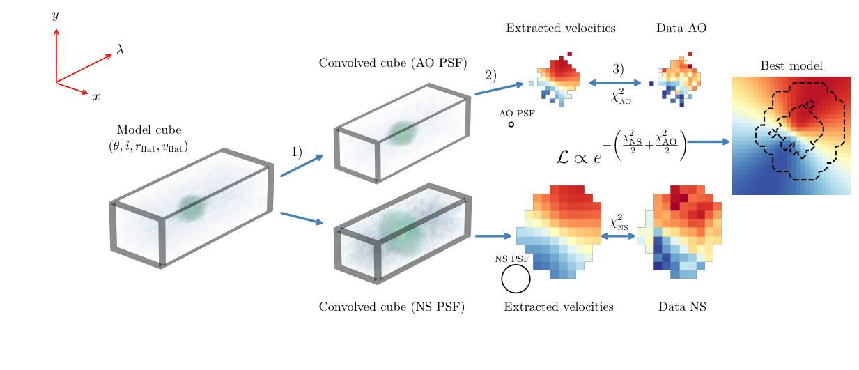
There are multiple advantages to this method. First, it makes use of the kinematic information of the same galaxy obtained with two instruments with different sensitivities, spatial resolutions and pixel scales. Second, the convolution with the respective PSF is done separately (but simultaneously), which helps mitigate the effects of systematic errors from single modelling. Lastly, this method gives the code the freedom to centre the two models at separate spatial locations so the possible differences in the alignment of the images (of a few pixels) are accounted for. We analyse the usefulness of this combination model-fitting method by comparing it to the single model fitting as discussed in Section 4.
4 Results and discussions.
| Galaxy | Data | ||||||||
|---|---|---|---|---|---|---|---|---|---|
| ID | Type | (∘) | (∘) | (kpc) | (kpc) | (km/s) | (km/s) | (kpc km/s) | (kpc km/s) |
| KMOS | |||||||||
| COSMOS 110446 | OSIRIS | ||||||||
| Combined | |||||||||
| KMOS | |||||||||
| COSMOS 171407 | OSIRIS | ||||||||
| Combined | |||||||||
| KMOS | |||||||||
| COSMOS 130477 | OSIRIS | ||||||||
| Combined | |||||||||
| KMOS | |||||||||
| COSMOS 127977 | OSIRIS | ||||||||
| Combined | |||||||||
| KMOS | |||||||||
| UDS 78317 | OSIRIS | ||||||||
| Combined | |||||||||
| KMOS | |||||||||
| COSMOS 08515 | SINFONI | ||||||||
| Combined | |||||||||
| KMOS | |||||||||
| GOODS-S 29868 | SINFONI | ||||||||
| Combined | |||||||||
| KMOS | |||||||||
| GOODS-S 33639 | SINFONI | ||||||||
| Combined | |||||||||
| KMOS | |||||||||
| GOODS-S 40218 | SINFONI | ||||||||
| Combined | |||||||||
| KMOS | |||||||||
| GOODS-S 42930 | SINFONI | ||||||||
| Combined |
The high-redshift sample studied in this paper is to date the largest sample with angular momentum measurements from the combination of high- and low-spatial resolution data. Consequently, we can address the relevance of a combination method. Throughout this section, we discuss the effect of combining the different resolutions in the determination of rotation velocity profiles, kinematic state as well as the convergence of to the asymptotic value . Table 3 shows the main results of the modelling and additional figures are included in the supplementary (online) section.

4.1 Classification as rotating disks
High-spatial resolution observations, to sub-kpc scales, are necessary to accurately determine the kinematic state of a galaxy and resolve large star-forming clumps. (Law et al. 2007; Genzel et al. 2008; Epinat et al. 2012; Livermore et al. 2015; Mieda 2015; Wisnioski et al. 2015; Fisher et al. 2017; Förster Schreiber et al. 2018; Sweet et al. 2019). In our full sample, the mean PSF FWHM of the adaptive optics sample ( arcsec) corresponds to kpc whereas the seeing-limited sample ( arcsec) corresponds to kpc. In the high-resolution data, additional components with proper line of sight velocities become visible as indicated in Figure 7.
Another way to assess the kinematic state of the sample is by determining the dynamical support using the ratio. Following Genzel et al. 2006, a system is considered dispersion supported for , and rotation supported for . However, as discussed by Tiley et al. 2019a, a galaxy is truly supported by its rotation when . In our sample, we use for the velocity and for the velocity dispersion we take the median of the annulus at in the moment two maps, where the effects of beam smearing are lower. The ratios at both resolutions are shown in Figure 8.
A commonly used approach to classify high-redshift galaxies as disks from their 2D kinematic maps (e.g Förster Schreiber et al. 2018; Wisnioski et al. 2019) consists of a set of criteria based on their rotation and dispersion profiles. These criteria (as proposed by Wisnioski et al. 2015) are:
1. a smooth monotonic velocity gradient across the galaxy, defining the kinematic axis;
2. a centrally peaked velocity dispersion distribution with maximum at the position of steepest velocity gradient, defining the kinematic centre;
3. dominant rotational support, quantified by the ratio;
4. co-aligned morphological and kinematic major axes (a.k.a. kinematic misalignment);
5. spatial coincidence of the kinematic and morphological centres.
We follow these criteria, the results from running the kinematic code and the visual inspection of the photometric maps to classify our sample: Galaxy UDS 78317 has four kinematic poles in the high-resolution map, the morphological and kinematic centres do not align, there is a large misalignment of the kinematic and morphological positions angles and it has a bright companion as seen in the HST images (see Figure 7), thus we classify it as a major merger in agreement with Sweet et al. 2019. GOODS-S 40218 is very compact and only a few pixels surpass the SNR threshold in the Gaussian fit at the two resolutions. Given these limitations, and based on the disordered velocities from both datasets and low ratios (1 for NS and 0.9 for AO), we classify this galaxy as a merger noting the large uncertainties. For the remainder of the analysis, we label these two galaxies in italics (UDS 78317 and GOODS-S 40218) throughout the paper to distinguish them from the rotating disks.
We treat COSMOS 171407 as a disk due to its ordered rotation but we note its complex structure in the AO H intensity map and a kinematic anomaly that is completely absent in its natural seeing counterpart, which is consistent with a minor merger. Galaxy GOODS-S 33639 has only a few pixels with enough SNR for the H Gaussian fit as well as poorly constrained inclinations from photometry and kinematics. However, it fulfils the conditions to be classified as a disk. The rest of the galaxies (COSMOS 110446, COSMOS 130477, COSMOS 127977, COSMOS 08515, GOODS-S 29868 and GOODS-S 42930) are classified as disks. In summary, 2/10 galaxies in our sample are classified as mergers (UDS 78317 and GOODS-S 40218), 8/10 are classified as disks with two of them (COSMOS 171407 and GOODS-S 33639) being largely uncertain. We discuss each individual case in further detail in the supplementary (online) section.

From similar disk/merger classifications, recent kinematic surveys have measured the fraction of disks () at cosmic noon and at later times. At an intermediate redshift range of , Epinat et al. 2012 found with the MASSIV survey for 50 star-forming galaxies, most of which were observed at low spatial resolution. Some larger (seeing-limited only) surveys at have found disk fractions as large as (e.g Wisnioski et al. 2015; Wisnioski et al. 2019; Stott et al. 2016). However, that range decreases to for the 35 galaxies assisted by adaptive optics studied in Förster Schreiber et al. 2018. Our results are consistent with those of the seeing limited surveys. However, it is worth noting that the five galaxies chosen from the KGES sub-sample () were galaxies that at low resolution appeared to be rotating, had flat rotation curves and well-behaved dispersion profiles. This introduces a selection bias, so the 1:5 ratio of galaxies misclassified as disks is a lower bound on this systematic uncertainty. For larger samples, with a wider range in parameter space, this ratio is likely to be higher.
4.2 Angular momentum measurements
We can use our angular momentum measurements to assess their consistency with known relations. One of these relations is the scaling of stellar specific angular momentum and stellar mass typically known as the “Fall relation” (Fall 1983). The power law that relates these quantities is well established at in the form with for disks and for bulges (Fall & Romanowsky 2018).
In Figure 9 we plot the eight disks in the vs map as well as the results from other studies that make predictions on the Fall relation at various redshift ranges (Fall & Romanowsky 2013; Swinbank et al. 2017; Posti et al. 2018; Gillman et al. 2020; Bouché et al. 2021). Since is measured more precisely using both resolutions (as shown in Appendix A), we use those values to find the scaling law that best describes the 8 disk galaxies (we exclude the mergers UDS 78317 and GOODS-S 40218). We use the relation where is the slope from the commonly used relation and is the normalization. In Table 4 we show the best-fit parameters to the unconstrained model (free and ) as well as a model with a fixed power-law slope .
From our small sample, we find a scatter of 0.38 dex, which occupies a similar parameter space in the vs relation as the majority of the measurements from Gillman et al. 2020 where they used 201 spatially resolved (seeing limited) galaxies at with a scatter of 0.56 dex. The constrained fit () to their sample has a small positive offset in the vertical axis () as compared to our constrained fit.
| Data | ||
|---|---|---|
| Constrained fit () | ||
| Unconstrained fit | ||
| KGES () | ||
| KGES unconstrained |
The small difference could be explained by the different mass distribution estimates from their photometric models which are more general (Sérsic models with ) than our assumed exponential disks (). There are also systematic differences associated to the chosen velocity profile, which in their case is measured at the kinematic position angle instead of the full velocity field. In their measurement, there could be objects that show ordered rotation at low resolution but that could be mergers when seen with high spatial resolution. We note that the limited number of objects in our sample and the small mass range provide little diagnostic ability on the slope of the vs relation.
According to the Fall relation, low- () galaxies have a low content so they are more susceptible to fragmentation due to a higher prevalence of galaxy-wide instabilities. Thus, they are better candidates for addressing the effect of angular momentum in driving clumpiness and are critical for constraining the low- regime in the vs relation. Constraints in the low-mass regime () of the Fall relation have been found at an intermediate redshift range () by Contini et al. 2016 and Bouché et al. 2021 using seeing-limited observations with the Multi Unit Spectroscopic Explorer (MUSE; Bacon et al. 2010). In our sample, the only galaxy with trustworthy results in the low- regime is COSMOS 08515. Part of the reason is that the sample is biased towards high-, as the targets chosen to be observed with adaptive optics with OSIRIS were the ones that appeared to be large disks with ordered rotation from the natural seeing observations in the KGES survey. A combined (NS+AO) analysis of galaxies in the low-mass regime is thus necessary to impose better constraints on the vs relation at the redshift of interest.
Another important measurement is the contribution of each data type in the total measurement of in terms of their spatial extent. In the combined analysis, we measure the contribution of the individual data sets by measuring the amount of angular momentum in the model enclosed within the boundaries of the high- and low-resolution maps respectively as shown in Figure 10. The adaptive optics data, with its sensitivity limitations, contributes to a mean value of of total whereas the natural seeing maps reach . The combination is thus ideal since the adaptive optics data aids a more precise measurement of the rotation profile in the inner radius, and natural seeing aids the measurement of the bulk of which is built at large radii, where the rotation curve is expected to flatten and the effects of beam smearing are smaller.
4.3 Uncertainties in the angular momentum measurements
In order to quantify the uncertainties in the measurement of associated with the individual and combined fits, we resample each galaxy times and run the same analysis for each iteration. To do this, we create a perfect model cube from the best-fit parameters using the pixel scale of the data and masking out empty pixels. We then convolve with the PSF and extract the velocity field from the convolved cube. Next, in order to recreate the observational errors, we take the residual velocity field (the difference between the best kinematic model and the real velocity field) and resample it with a normal distribution in each pixel. This new error map is then added to the model velocity field. This empirical approach better captures the contribution of artifacts and substructure that are not covered by the kinematic model, since they manifest in the residual velocity fields. If we used the Gaussian line fit errors instead, we would get unrealistically low uncertainties since the residuals are typically 0-70 km/s compared to the formal errors of km/s from the Gaussian line fits. We also resample the photometric model, where the noise is estimated from the RMS of the background regions in the HST images.
For each realization of the model, we recalculate in the individual and combined cases with the advantage of knowing the actual value of from the input model . The scatter in the deviations from this real value will give us an estimation of how good the measurement is in each case. This exercise quantifies the random error that would be obtained if a galaxy corresponding to the best fit model was observed with the same data mask, substructure and similar noise levels. It also allows us to assess the systematic error levels in the methodology.
The systematic error in for each galaxy is calculated from the median of the errors from the 100 realizations of the model. For the full sample, the average systematic errors are for the natural seeing data, for the adaptive optics data and in the combination. More importantly, by taking the standard deviation of the individual errors from the realizations we obtain the error for each galaxy as well as the errors in all parameters reported in Table 3. The mean percentage error for the measurements using natural seeing data is 49%, in the case of adaptive optics 26.5% and as for the combined resolutions it is 16% as shown in Figure 11. This clear improvement can be explained by the better constraints imposed in the inner part of the rotation curves where the adaptive optics data is essential as well as the larger spatial extent of the combined data.
4.4 Geometrical parameters
We pay special attention in determining the position angle and inclination as they are critical quantities in the deprojection of the velocity field. In the case of the inclination, there is a well-known degeneracy between rotation velocity and inclination that arises from kinematic modelling alone (e.g. Begeman 1989; Epinat et al. 2010; Kamphuis et al. 2015; Bekiaris et al. 2016). In order to break this degeneracy, and noting that the uncertainty in the inclinations is one of the largest caveats in our analysis, we adopt a consistent approach to that of Swinbank et al. 2017 for relative comparison where we constrain the inclination from the galaxies’ surface brightness profiles as done by other kinematic codes (e.g. Bouché et al. 2015, GalPaK3D,). For axisymmetric disk-like galaxies, the axis ratio can be used to estimate the inclination (Holmberg 1946) as:
| (6) |
where is the observed axis ratio and is the true axis ratio of an edge on system that depends on morphological type (Heidmann et al. 1972; Fouque et al. 1990). In the thin-disk approximation , so this relation reduces to , however, star-forming galaxies at high redshift show vertical dispersion (Law et al. 2007; Förster Schreiber et al. 2009) that corresponds to thick disks with so we adopt this value for consistency with previous studies at high redshift (e.g. Wisnioski 2012; Harrison et al. 2017; Gillman et al. 2020).
We compare the inclinations measured individually from photometry () and from the kinematic modelling alone () where we find that the kinematic modelling underestimates the inclinations for 8/10 of the galaxies in the sample as seen in Figure 12. The values of of those eight galaxies are low , where the degeneracy with the velocity field (characterized by ) escalates more rapidly as discussed by Bekiaris et al. 2016. This degeneracy leads to an increase on the parameter and thus an overall increase in the measurements of . Besides the known degeneracy, such low inclinations deviate significantly from the mean expected inclination of disk galaxies given their random orientations in space. Following geometrical arguments, this mean expected value is (see Appendix of Law et al. 2009) which is consistent with the mean value of the photometric inclinations (and bootstrap errors) of our sample . On the other hand, the mean kinematic inclinations largely disagree with .
Moreover, the predictions on the Fall relation are significantly different when using the kinematic or photometric inclinations. If we used best fit parameters from the kinematic model alone (without constraining the inclination from photometry), we find a zero-point of 2.75 for the fixed power slope , which has a positive 0.23 offset with the with respect to the fit with the photometric inclinations. This experiment confirms the necessity of imposing constraints in the inclinations from the surface brightness profiles.
In the case of the position angle , we used the values measured from the kinematic modelling since the equivelocity contours of the “spider diagram” (e.g. fourth column in Figure 5) are indicative of a clear main axis. On the other hand, the position angle estimated from photometry depends on the light distribution which is more susceptible to global non-axisymmetric features within the disk (Palunas & Williams 2000). The from kinematics is thus better constrained, especially in the combined case.
The misalignment between and can be a product of physical differences such as bright clumps in the continuum, the asymmetry between the stellar and gas distributions as well as complex morphologies due to mergers (Rodrigues et al. 2017). However, it can also be a product of the lack of precision in the deprojection of high redshift maps. We find that the galaxies that show the largest misalignment are the two mergers and the galaxy with large uncertainties (GOODS-S 33639) as indicated in Figure 13, which is consistent with the disk-merger criteria discussed in Section 4.1. For the rest of the sample, there is an overall agreement in the position angles which supports the choice of using the photometric inclinations.
4.5 Angular momentum convergence
Stellar specific angular momentum converges to an asymptotic value at large radii, with some notable differences between the different resolutions. A direct comparison of the convergence at different radii (namely ) between the different data types shows that the measured converges faster in the case of the high-resolution data as shown in Figure 14. This result is expected since the rapidly growing rotation curves are better determined with the high-resolution data in the centre of the disks, whereas the flat part of the rotation curve is better determined with the seeing limited data where the effects of beam smearing are smaller.
Another consistent result that we find throughout the whole sample is that the approximation (Equation 5), agrees within with the total angular momentum value measured from the best fit models in the combined analysis as in Figure 15. This approximation relies on global variables that can be measured from low-resolution data such as the galaxy size and asymptotic velocity, hence natural seeing observations can provide a good estimation of the total angular momentum content of galaxies that are indeed disks as suggested by Romanowsky & Fall 2012.
4.6 Comparison with Natural-seeing based results
We test the reliability of natural-seeing based estimations of by comparing them with those from the combined analysis. In order to do that, we measure the ratio of both quantities as a function of disk scale length as shown in Figure 16, where no dependence on redshift or galaxy size was found.
We find that the NS-only measurements of for the disk galaxies are within 10% from the combined ones (with the exception of COSMOS 0851588 8 The large discrepancy is due to the dramatic difference between the values of , which is more prominently affected by beam smearing in the case of the NS fit (it has the lowest spatial resolution in the full sample with PSF FWHM = 0.966 arcsec).), suggesting that if the galaxies are truly disks, then the natural seeing based estimations of are reliable. However, in the case of the two galaxies classified as mergers, the discrepancy in the measurement is large (), which shows how the poor determination of the real kinematic state of the galaxy (from low resolution) can lead to under- or over-estimations of . Even if the estimation of from the combined analysis of those galaxies is also wrong (as the calculation is still done assuming an exponential disk with ordered rotation), the large difference between the two measurements could be used as an indicator of a complex kinematic state for future large samples.
In order to compare our results with other existing low-resolution studies and directly address the possible systematics associated with our chosen method, we compare our individual measurements to those obtained for the KGES sample by Gillman et al. 2020 for the five galaxies at that overlap with our sample. We compare their measurements with our natural-seeing only measurements (as well as the combined resolutions) as shown in Figure 17. This is not a fully direct comparison since the functional form they used to measure is different from ours but it allows to identify the systematic differences between the two approaches. The values in Gillman et al. 2020 are obtained with the approximation (Equation 5) where is measured from a Sérsic fit with GALFIT and is obtained from a parametric model that can rise or decline at large radii99 9 This parametric model of the rotation velocity is based on an exponential light profile so it is characterized by the scale length of an exponential disk (Equation 10 in Freeman 1970).. Since the KGES values of are measured at , where beam smearing effects are low, they are similar to our measurement at the level.
We find that the large differences in the galaxy size measurement (shown in Table 5) directly translate into the large discrepancies of our measurements with the values. For the galaxies where our measurement of is significantly larger ( 75%) (COSMOS 110446, COSMOS 127977 and COSMOS 171407), the ratios in are also significantly larger, whereas for the galaxies where the measurement of is smaller ( 50%) (COSMOS 130477 and UDS 78317), the value is smaller as well.
The large difference in galaxy sizes can be attributed to the different surface brightness profiles used in each case (Sérsic profile with varying in Gillman et al. 2020 and exponential disk in our analysis) because the radius enclosing half of the light depends strongly on the power-law slope. This implies that an erroneous fit of the Sérsic index , which could be caused by the low resolution of the HST maps and clumpy nature of these galaxies, can lead to over or underestimations of the light profile as well as unrealistic values of . For example, the steep gradient in SNR could bias the fit to smaller values of (steep profile), and thus bias the fit to small values of . In fact, some of the Sérsic fits, particularly those with , are at the limit of the fitting range and thus the estimations of the galaxy size are unreliable. In our analysis, we chose the exponential profile, which has a shallower slope and thus contains a large fraction of the galaxy light in the outskirts, where the SNR of the data is low. For 6/10 galaxies, the (average) radial surface brightness profile has lower RMS residuals when using the exponential disk assumption as compared to the Sérsic fit as shown for each individual galaxy in Figures S1 to S6 in the supplementary section.
The comparison to the results of the KGES sample also allows us to determine the intrinsic scatter in the vs relation. The RMS scatter of the KGES seeing-limited sample is dex whereas for our eight disks we get dex. Even though a sample of eight disks is not enough to make statistically significant predictions, we note that this is still a large scatter, suggesting that adding the high-resolution kinematic data does have a significant effect on it. This could indicate that the observed scatter found from low resolution studies is not related to systematic effects caused by poor resolution. Instead, this intrinsic scatter could be attributed to different mechanisms of retention and redistribution of angular momentum due to inflows and outflows, morphological differences, varied bulge-to-total fractions, and complex environmental conditions such as higher incidence of minor mergers and large gas accretion from cosmic filaments. In the local Universe, the RMS scatter of the parametric relation of disks decreases to dex (e.g. Romanowsky & Fall 2012; Obreschkow & Glazebrook 2014b; Posti et al. 2018), pointing to the emerging of rotational support that assembles massive disks in the local Universe (Simons et al. 2017).
| Galaxy | (kpc) | (kpc) | ||
| ID | Gillman et al. 2020 | (this work) | ||
| COSMOS 110446 | 1.08 | 0.5 | 2.35 | |
| COSMOS 171407 | 2.13 | 0.2 | 4.03 | |
| COSMOS 130477 | 2.75 | 1.1 | 4.03 | |
| COSMOS 127977 | 2.06 | 0.2 | 3.69 | |
| UDS 78317 | 4.07 | 0.4 | 3.02 | |
| Tacchella et al. 2015 | (this work) | |||
| COSMOS 08515 | 2.2 | 0.5 | 4.9 | |
| GOODS-S 29868 | 5.7 | 0.2 | 4.7 | |
| GOODS-S 33639 | 3.6 | 0.6 | 5.0 | |
| GOODS-S 40218 | 1.3 | 0.9 | 1.8 | |
| GOODS-S 42930 | 1.7 | 1.3 | 2.7 | |
4.7 Effects of galaxy clumpiness
The precision of a direct pixel-by-pixel measurement of from the actual data is limited by the number of pixels with useful information in and as well as their difference in pixel scales and spatial resolutions (this motivated the use of the analytical calculation from Equation 2). However, it can be useful when trying to avoid bias from assumed models. In the case of the photometry, extensive star-formation activity in bright clumps (not necessarily massive) within the disks and a central bulge can affect the observed morphology from the HST maps which is not accounted for in the exponential disk assumption. We calculate the pixel-by-pixel stellar specific angular momentum of all galaxies as
| (7) |
where go through all the spatially-matched pixels in velocity and photometry. In order to quantify the effects of clumpiness as well as the chosen form of , we perform four separate experiments (the first three are shown in Figure 18) that we explain in the following paragraphs.
i) Using HST data instead of the I(x,y) model: We take the measurement of where and come from the best-fit models and compare it to the measurement where comes from the HST data directly. Galaxies COSMOS 110446, COSMOS 130477, COSMOS 127977, UDS 78317 and GOODS-S 29868 show a large difference at the difference level (with using the HST being higher), likely due to the multiple bright components located away from the centre in their HST maps. The difference in the rest of the galaxies is at the level. The majority of the light coming from the bright regions comes from young stellar populations that ionize the surrounding gas, so it only represents a small fraction of the full mass content. Hence if these clumps are young, then the assumption that light traces mass provides an upper bound in the systematic error which is at the level for the whole sample.
ii) Using a Sérsic profile (in 2D) instead of the exponential profile (in 2D): Another way to test the systematics associated with the choice of surface brightness profile is by using a Sérsic profile instead of the exponential disk. We use the best-fit parameters from Gillman et al. 2020 and Tacchella et al. 2015 to create the models from where we find large differences throughout the whole sample with the majority of the ratios being larger than unity (model yields larger ratios than Sérsic profile ) except for the merger UDS 78317 and GOODS-S 29868 which are the only galaxies where from the exponential disk fit is lower as seen in Table 5. In particular, we find dramatic differences at the >50% level for six galaxies with COSMOS 110446 and COSMOS 171407 being the most extreme cases with ratios of 3.2 and 2.5 respectively. As mentioned in the previous subsection, despite the generalities that a Sérsic profile allows, steep gradients in the poorly-constrained light profiles can lead to small values of which translate to lower values of and thus underestimate the total value of .
iii) 2D approach vs 1D analytical calculation: In addition to testing the systematics associated with the assumed model, we compare the pixel-by-pixel measurement with the estimation from the one-dimensional analytical expression in Equation 2. We find a strong dependence in the disk scale length as the analytic calculation deviates significantly () in the case of COSMOS 08515 and GOODS-S 33639 which have the largest (2.9 and 3 kpc respectively). On the other hand, the galaxies where the difference in is (COSMOS 110446, UDS 78317, GOODS-S 40218 and GOODS-S 42930) are the galaxies with the lowest with kpc. This scale dependence can be attributed to the error introduced by the discrete change in intensities (and velocities) from the pixel-by-pixel approach. This effect is stronger when is large since more pixels will have values that deviate more from the analytical expression which is more reliable since it depends only on , and .
iv) Bulge and clumps contribution: We quantify the effect of adding a central bulge in the modelling that follows a Sérsic profile with and a size of kpc in our modelling. The choice of this size is motivated by the findings of Fisher & Drory 2010 who estimate typical bulge sizes in the local Universe and the bulge-disk decomposition performed in Tacchella et al. 2015 on the SINS galaxies where they find typical bulge sizes of kpc. We recalculate with the modified mass distribution model while keeping the same velocity field information (since it is constrained by the multiple resolutions). We add the extra co-rotating component by varying the bulge-to-total ratio in the range [0.1-0.5], noting that in the decomposition on J- and H-band HST images performed by Tacchella et al. 2015 on COSMOS 08515, GOODS-S 33639, GOODS-S 40218 and GOODS-S 42930, the bulge-to-total ratios were all in the range [0-0.3].
For a constant mass-to-light ratio , we find that the effect of the bulge is a decrease in the total measurement of , in consistency with similar studies (e.g. Romanowsky & Fall 2012; Obreschkow & Glazebrook 2014b). The effect is minimal at with a small median decrease in of , and becomes more prominent at higher , having the maximum effect at of with a median decrease of 10% in . However, since the stellar populations in the bulge are different from those in the disk, then the in each component is different as well. In order to quantify this effect, we make use of the J- and H- band HST data at used in Tacchella et al. 2015 (via private communication) to perform a color analysis. Since J-H colors at correspond to rest-frame u-g, we can use them as a proxy for stellar mass-to-light ratios based on color- relations (Bell & de Jong 2001). From the radial color profiles and color maps we find color differences in the bulge and disk of which translate to bulges that are more massive than the disk using the relations in Bell et al. 2003. This difference sets an upper bound of , and shows that galaxies with massive central bulges (higher mass-to-light ratios) have a lower content of stellar specific angular momentum.
A similar color analysis of the galaxies with the most prominent clumps and high quality HST multi-wavelength data (namely COSMOS 08515 and GOODS-S 29868), sets an upper bound on the effect of their bright clumps on the overall measurement of . From the color maps, we identify clumps that are bluer (younger) than the disk with a maximum difference of which translates to a difference in mass-to-light ratio of . Thus, these clumps are 50% less massive than their host disks so they contribute less to the mass profile of the galaxy. In parallel to the effect of the bulge, the effect of these young clumps in is a slight decrease of 8% for COSMOS 08515 (with two clumps) and 5% for GOODS-S 29868 (one clump), where we have used clump sizes of kpc from the HST broad-band imaging at their distance from the galaxy centre. The measurement of this effect is limited to the difference in mass profile as we did not include any extra kinematic components in the model. Besides its consistency with similar studies, this assumption is justified from the inspection of the velocity fields which show no significant differences in the regions where these clumps reside (they appear to co-rotate with the disks). For the rest of the sample, this contribution () is expected to be of similar order so it does not have a dramatic effect on the stellar specific angular momentum measurements in this work.
5 Conclusions
We have gathered and analysed a sample of 10 high-redshift ( and ) galaxies that have IFS observations at high and low spatial resolution as well as near-infrared HST observations to measure their stellar specific angular momentum content. This is the largest sample to date with angular momentum measurements coming from the combination of adaptive optics assisted observations and their seeing limited counterparts. We summarize our findings as follows:
- •
We developed a code to combine and take advantage of the different capabilities of each data type (adaptive optics provides high resolution but low sensitivity and natural seeing provides low resolution but high sensitivity). In the “2D” modelling we carefully apply the right convolution to each model cube and find the best model using a maximum likelihood technique. We successfully tested the kinematic code by simulating a sample of mock galaxies with similar characteristics and running the code at different resolutions. Besides providing a sanity check for the code, it also confirmed that the combination of the different resolutions reduces the uncertainty in as explained in Appendix A.
- •
In order to increase SNR in two of the adaptive optics assisted datacubes, we employed different spatial smoothing methods and the median filter provided the best results. The signal was improved sufficiently so that H emission could be used to measure its emission line kinematics and the spatial resolution was kept high enough to improve that of seeing limited data.
- •
We have measured the improvement in the uncertainties of by resampling the models with a Monte Carlo approach. The mean uncertainties in the sample are 49% in the natural seeing case, 26.5% for adaptive optics and 16% when combining the datasets. The improvement comes from a reduction in the effects of beam smearing and the accurate modelling of the rotation curves, which are expected to rise rapidly in the inner regions of disk galaxies (better determined with adaptive optics) and then flatten at large radii (better determined with the deeper seeing limited counterpart). The combination can thus improve the measurements of that come from large seeing-limited surveys and will be more useful once large samples of adaptive optics assisted measurements are made with upcoming facilities such as JWST and next generation ground-based IFUs.
- •
Estimates of from the natural seeing observations are reliable (within of the combined analysis) when the galaxies are confidently classified as disks. The only exception was galaxy COSMOS 08515 due to the very poor resolution in NS. This suggests that the reliability of the findings from large seeing limited surveys depends strongly on the accurate kinematic classification of the samples.
- •
Besides the measurement from the best-fit models, we calculate the stellar specific angular momentum of all galaxies with a widely used approximation in terms of the rotation profile and size of the disk. This value labeled consistently agrees with the asymptotic angular momentum measurement obtained from the full modelling within 20%.
- •
A pixel-by-pixel measurement is subject to large systematic uncertainties due to resolution effects and pixel scales. A smooth profile assumption from an analytical calculation of can reduce the effect of these systematics and its reliability depends on the choice of surface brightness and rotation velocity profiles. In particular, the size is a critical quantity in measuring and depends strongly on the choice of .
- •
We classify GOODS-S 40218 and UDS 78317 as mergers. The latter was previously defined as a rotating disk from natural seeing only studies but turned out to be a merger from the high-resolution observations, in accordance with Sweet et al. 2019. We find that two of the other systems (COSMOS 171407 and GOODS-S 33639) have complex H intensity and kinematic structures but insufficient to catalog them as mergers so we treat them as disks. The other six galaxies are classified as rotating disks.
- •
We used the eight galaxies identified as disks to make a prediction on the Fall relation ( vs ). We find that our best fit with a constrained slope agrees with the findings of previous high-redshift studies within dex. This is limited by the small number of galaxies in our current sample. A direct comparison to the relation found from a seeing limited sample at a similar redshift (Gillman et al. 2020 at ) shows a minor offset, despite the differences in the methods used to measure (different mass distributions and radial extents).
- •
The scatter of our measurements in the Fall relation remains large ( dex) even in the combined analysis in similarity with the “NS-only” analysis of Gillman et al. 2020. The scatter is thus intrinsic and reflects diversity in galaxy assembly and complex morphology where stellar bulge-to-total ratios may play a more important role. In the local Universe, the scatter decreases to pointing to the assembly of disks through rotational support.
In future work, we will apply the method introduced here on a larger sample from the seeing limited survey Förster Schreiber et al. 2009 with its adaptive optics counterparts from Förster Schreiber et al. 2018. This will expand the current combined analysis to a low-mass regime and will provide further constraints in the vs relation from multi-resolution measurements of .
Acknowledgements
We thank the anonymous referee for helpful comments and suggestions that greatly improved this manuscript. JE is funded by the Swinburne University Postgraduate Research Award (SUPRA). JE, DBF, KG, DO and SMS acknowledge support from Australian Research Council (ARC) DP grant DP160102235. DBF acknowledges support from ARC Future Fellowship FT170100376. DO is a recipient of an ARC Future Fellowship (FT190100083) funded by the Australian Government. ALT acknowledges support from a Forrest Research Foundation Fellowship. SG acknowledges the support of the Science and Technology Facilities Council through grant ST/N50404X/1 and ST/L00075X/1 for support and the Cosmic Dawn Centre of Excellence funded by the Danish National Research Foundation under grant No. 140. Some of the data presented herein were obtained at the W. M. Keck Observatory, which is operated as a scientific partnership among the California Institute of Technology, the University of California and NASA. The Observatory was made possible by the generous financial support of the W. M. Keck Foundation. The KMOS data were obtained at the Very Large Telescope of the European Southern Observatory, Paranal, Chile, and provided by the KGES survey team and the public release of KMOS3D. The SINFONI data were obtained at the same facility and provided in the public release of the SINS/zC-AO survey. HST data were obtained from the data archive at the Space Telescope Science Institute. Simulations in this work were performed on the OzStar national facility at Swinburne University of Technology and the National Collaborative Research Infrastructure Strategy (NCRIS). We acknowledge the open-source software packages used throughout this work including astropy (Astropy Collaboration et al. 2013), scipy (Virtanen et al. 2019), numpy (van der Walt et al. 2011), CMasher (van der Velden 2020), matplotlib (Hunter 2007).
6 Data availability
The data underlying this article will be shared on reasonable request to the corresponding author.
References
- Airy (1835) Airy G. B., 1835, Transactions of the Cambridge Philosophical Society, 5, 283
- Astropy Collaboration et al. (2013) Astropy Collaboration et al., 2013, A&A, 558, A33
- Avila (2017) Avila R. J., 2017, Advanced Camera for Surveys Instrument Handbook for Cycle 25 v. 16.0
- Bacon et al. (2010) Bacon R., et al., 2010, in McLean I. S., Ramsay S. K., Takami H., eds, Society of Photo-Optical Instrumentation Engineers (SPIE) Conference Series Vol. 7735, Ground-based and Airborne Instrumentation for Astronomy III. p. 773508, doi:10.1117/12.856027
- Bassett et al. (2014) Bassett R., et al., 2014, MNRAS, 442, 3206
- Begeman (1989) Begeman K. G., 1989, A&A, 223, 47
- Bekiaris et al. (2016) Bekiaris G., Glazebrook K., Fluke C. J., Abraham R., 2016, Monthly Notices of the Royal Astronomical Society, 455, 754
- Bell & de Jong (2001) Bell E. F., de Jong R. S., 2001, ApJ, 550, 212
- Bell et al. (2003) Bell E. F., McIntosh D. H., Katz N., Weinberg M. D., 2003, ApJS, 149, 289
- Bellocchi et al. (2012) Bellocchi E., Arribas S., Colina L., 2012, A&A, 542, A54
- Bezanson et al. (2018) Bezanson R., et al., 2018, ApJ, 858, 60
- Blumenthal et al. (1984) Blumenthal G. R., Faber S., Primack J. R., Rees M. J., 1984, Nature, 311, 517
- Boissier et al. (2003) Boissier S., Prantzos N., Boselli A., Gavazzi G., 2003, MNRAS, 346, 1215
- Bouché et al. (2007) Bouché N., et al., 2007, ApJ, 671, 303
- Bouché et al. (2015) Bouché N., Carfantan H., Schroetter I., Michel-Dansac L., Contini T., 2015, AJ, 150, 92
- Bouché et al. (2021) Bouché N. F., et al., 2021, arXiv e-prints, p. arXiv:2101.12250
- Burkert et al. (2016) Burkert A., et al., 2016, ApJ, 826, 214
- Carignan et al. (2006) Carignan C., Chemin L., Huchtmeier W. K., Lockman F. J., 2006, ApJ, 641, L109
- Catelan & Theuns (1996a) Catelan P., Theuns T., 1996a, Monthly Notices of the Royal Astronomical Society, 282, 436
- Catelan & Theuns (1996b) Catelan P., Theuns T., 1996b, MNRAS, 282, 455
- Catinella et al. (2006) Catinella B., Giovanelli R., Haynes M. P., 2006, ApJ, 640, 751
- Conselice et al. (2000) Conselice C. J., Bershady M. A., Jangren A., 2000, ApJ, 529, 886
- Contini et al. (2016) Contini T., et al., 2016, A&A, 591, A49
- Cortese et al. (2016) Cortese L., et al., 2016, Monthly Notices of the Royal Astronomical Society, 463, 170
- Cresci et al. (2009) Cresci G., et al., 2009, Astrophysical Journal, 697, 115
- Davies & Kasper (2012) Davies R., Kasper M., 2012, ARA&A, 50, 305
- Decarli et al. (2019) Decarli R., et al., 2019, ApJ, 882, 138
- Dekel & Burkert (2014) Dekel A., Burkert A., 2014, MNRAS, 438, 1870
- Dekel et al. (2009) Dekel A., Sari R., Ceverino D., 2009, ApJ, 703, 785
- Eisenhauer et al. (2003) Eisenhauer F., et al., 2003, in Iye M., Moorwood A. F. M., eds, Society of Photo-Optical Instrumentation Engineers (SPIE) Conference Series Vol. 4841, Instrument Design and Performance for Optical/Infrared Ground-based Telescopes. pp 1548–1561 (arXiv:astro-ph/0306191), doi:10.1117/12.459468
- Elmegreen et al. (2005) Elmegreen D. M., Elmegreen B. G., Rubin D. S., Schaffer M. A., 2005, ApJ, 631, 85
- Epinat et al. (2010) Epinat B., Amram P., Balkowski C., Marcelin M., 2010, Monthly Notices of the Royal Astronomical Society, 401, 2113
- Epinat et al. (2012) Epinat B., et al., 2012, A&A, 539, A92
- Fall (1983) Fall S. M., 1983, in Athanassoula E., ed., Vol. 100, Internal Kinematics and Dynamics of Galaxies. pp 391–398
- Fall & Efstathiou (1980) Fall S. M., Efstathiou G., 1980, MNRAS, 193, 189
- Fall & Romanowsky (2013) Fall S. M., Romanowsky A. J., 2013, ApJ, 769, L26
- Fall & Romanowsky (2018) Fall S. M., Romanowsky A. J., 2018, ApJ, 868, 133
- Fisher & Drory (2010) Fisher D. B., Drory N., 2010, ApJ, 716, 942
- Fisher et al. (2017) Fisher D. B., et al., 2017, MNRAS, 464, 491
- Foreman-Mackey et al. (2013) Foreman-Mackey D., Hogg D. W., Lang D., Goodman J., 2013, PASP, 125, 306
- Förster Schreiber et al. (2009) Förster Schreiber N. M., et al., 2009, ApJ, 706, 1364
- Förster Schreiber et al. (2018) Förster Schreiber N. M., et al., 2018, ApJS, 238, 21
- Fouque et al. (1990) Fouque P., Bottinelli L., Gouguenheim L., Paturel G., 1990, ApJ, 349, 1
- Freeman (1970) Freeman K. C., 1970, ApJ, 160, 811
- Genzel et al. (2006) Genzel R., et al., 2006, Nature, 442, 786
- Genzel et al. (2008) Genzel R., et al., 2008, ApJ, 687, 59
- Giavalisco et al. (2004) Giavalisco M., et al., 2004, ApJ, 600, L93
- Gillman et al. (2019) Gillman S., et al., 2019, MNRAS, 486, 175
- Gillman et al. (2020) Gillman S., et al., 2020, MNRAS, 492, 1492
- Glazebrook (2013) Glazebrook K., 2013, Publications of the Astronomical Society of Australia, 30, e056
- Glazebrook et al. (1995) Glazebrook K., Ellis R., Santiago B., Griffiths R., 1995, MNRAS, 275, L19
- Guérou et al. (2017) Guérou A., et al., 2017, A&A, 608, A5
- Harrison et al. (2017) Harrison C. M., et al., 2017, MNRAS, 467, 1965
- Heidmann et al. (1972) Heidmann J., Heidmann N., de Vaucouleurs G., 1972, Mem. RAS, 75, 85
- Holmberg (1946) Holmberg E., 1946, Meddelanden fran Lunds Astronomiska Observatorium Serie II, 117, 3
- Hubble (1926) Hubble E., 1926, Contributions from the Mount Wilson Observatory / Carnegie Institution of Washington, 324, 1
- Hunter (2007) Hunter J. D., 2007, Computing in Science & Engineering, 9, 90
- Józsa et al. (2007) Józsa G. I. G., Kenn F., Klein U., Oosterloo T. A., 2007, A&A, 468, 731
- Kamphuis et al. (2015) Kamphuis P., Józsa G. I. G., Oh S. . H., Spekkens K., Urbancic N., Serra P., Koribalski B. S., Dettmar R. J., 2015, MNRAS, 452, 3139
- Koekemoer et al. (2011) Koekemoer A. M., et al., 2011, ApJS, 197, 36
- Krajnović et al. (2006) Krajnović D., Cappellari M., de Zeeuw P. T., Copin Y., 2006, MNRAS, 366, 787
- Larkin et al. (2006) Larkin J., et al., 2006, in Society of Photo-Optical Instrumentation Engineers (SPIE) Conference Series. p. 62691A, doi:10.1117/12.672061
- Law et al. (2007) Law D. R., Steidel C. C., Erb D. K., Larkin J. E., Pettini M., Shapley A. E., Wright S. A., 2007, ApJ, 669, 929
- Law et al. (2009) Law D. R., Steidel C. C., Erb D. K., Larkin J. E., Pettini M., Shapley A. E., Wright S. A., 2009, ApJ, 697, 2057
- Lawrence et al. (2007) Lawrence A., et al., 2007, MNRAS, 379, 1599
- Liao et al. (2017) Liao S., Gao L., Frenk C. S., Guo Q., Wang J., 2017, MNRAS, 470, 2262
- Livermore et al. (2015) Livermore R. C., et al., 2015, MNRAS, 450, 1812
- Madau & Dickinson (2014) Madau P., Dickinson M., 2014, ARA&A, 52, 415
- Marasco et al. (2019) Marasco A., Fraternali F., Posti L., Ijtsma M., Di Teodoro E. M., Oosterloo T., 2019, Astronomy and Astrophysics
- Markwardt (2009) Markwardt C. B., 2009, in Bohlender D. A., Durand D., Dowler P., eds, Astronomical Society of the Pacific Conference Series Vol. 411, Astronomical Data Analysis Software and Systems XVIII. p. 251 (arXiv:0902.2850)
- Mieda (2015) Mieda E., 2015, PhD thesis, University of Toronto
- Mo et al. (1998) Mo H. J., Mao S., White S. D. M., 1998, MNRAS, 295, 319
- Mobasher et al. (2015) Mobasher B., et al., 2015, ApJ, 808, 101
- Moffat (1969) Moffat A. F. J., 1969, A&A, 3, 455
- Mowla et al. (2019) Mowla L. A., et al., 2019, ApJ, 880, 57
- Naab & Ostriker (2017) Naab T., Ostriker J. P., 2017, ARA&A, 55, 59
- Obreschkow & Glazebrook (2014a) Obreschkow D., Glazebrook K., 2014a, ApJ, 784, 26
- Obreschkow & Glazebrook (2014b) Obreschkow D., Glazebrook K., 2014b, ApJ, 784, 26
- Obreschkow et al. (2015) Obreschkow D., et al., 2015, ApJ, 815, 97
- Palunas & Williams (2000) Palunas P., Williams T. B., 2000, AJ, 120, 2884
- Peebles (1969) Peebles P. J. E., 1969, ApJ, 155, 393
- Pichon et al. (2011) Pichon C., Pogosyan D., Kimm T., Slyz A., Devriendt J., Dubois Y., 2011, MNRAS, 418, 2493
- Posti et al. (2018) Posti L., Fraternali F., Di Teodoro E. M., Pezzulli G., 2018, A&A, 612, L6
- Rodrigues et al. (2017) Rodrigues M., Hammer F., Flores H., Puech M., Athanassoula E., 2017, MNRAS, 465, 1157
- Romanowsky & Fall (2012) Romanowsky A. J., Fall S. M., 2012, ApJS, 203, 17
- Scoville et al. (2007) Scoville N., et al., 2007, ApJS, 172, 1
- Sellwood & Spekkens (2015) Sellwood J. A., Spekkens K., 2015, arXiv e-prints, p. arXiv:1509.07120
- Sharples et al. (2013) Sharples R., et al., 2013, The Messenger, 151, 21
- Simon et al. (2003) Simon J. D., Bolatto A. D., Leroy A., Blitz L., 2003, ApJ, 596, 957
- Simons et al. (2017) Simons R. C., et al., 2017, ApJ, 843, 46
- Simons et al. (2019) Simons R. C., et al., 2019, The Astrophysical Journal, 874, 59
- Stott et al. (2016) Stott J. P., et al., 2016, MNRAS, 457, 1888
- Sweet et al. (2019) Sweet S. M., et al., 2019, MNRAS, 485, 5700
- Swinbank et al. (2017) Swinbank A. M., et al., 2017, MNRAS, 467, 3140
- Szomoru et al. (2011) Szomoru D., Franx M., Bouwens R. J., van Dokkum P. G., Labbé I., Illingworth G. D., Trenti M., 2011, ApJ, 735, L22
- Tacchella et al. (2015) Tacchella S., et al., 2015, ApJ, 802, 101
- Tacchella et al. (2016) Tacchella S., Dekel A., Carollo C. M., Ceverino D., DeGraf C., Lapiner S., Mand elker N., Primack Joel R., 2016, MNRAS, 457, 2790
- Tacconi et al. (2013) Tacconi L. J., et al., 2013, ApJ, 768, 74
- Teklu et al. (2015) Teklu A., Remus R., Dolag K., Beck A., Burkert A., Schmidt A., Schulze F., Steinborn L., 2015, The Astrophysical Journal, 812
- Teuben (2004) Teuben P. J., 2004, in Ochsenbein F., Allen M. G., Egret D., eds, Astronomical Society of the Pacific Conference Series Vol. 314, Astronomical Data Analysis Software and Systems (ADASS) XIII. p. 621
- Tiley et al. (2019a) Tiley A. L., et al., 2019a, MNRAS, 482, 2166
- Tiley et al. (2019b) Tiley A. L., et al., 2019b, MNRAS, 485, 934
- Tiley et al. (2021) Tiley A. L., et al., 2021, MNRAS, 506, 323
- Tully & Fisher (1977) Tully R. B., Fisher J. R., 1977, A&A, 500, 105
- Ventou et al. (2017) Ventou E., et al., 2017, A&A, 608, A9
- Ventou et al. (2019) Ventou E., et al., 2019, A&A, 631, A87
- Virtanen et al. (2019) Virtanen P., et al., 2019, arXiv e-prints, p. arXiv:1907.10121
- Wechsler & Tinker (2018) Wechsler R. H., Tinker J. L., 2018, ARA&A, 56, 435
- Whitaker et al. (2019) Whitaker K. E., et al., 2019, ApJS, 244, 16
- Wisnioski (2012) Wisnioski E., 2012, PhD thesis, Swinburne University of Technology
- Wisnioski et al. (2015) Wisnioski E., et al., 2015, ApJ, 799, 209
- Wisnioski et al. (2019) Wisnioski E., et al., 2019, ApJ, 886, 124
- Zasov et al. (2017) Zasov A. V., Saburova A. S., Khoperskov A. V., Khoperskov S. A., 2017, Physics Uspekhi, 60, 3
- de Blok et al. (2008) de Blok W. J. G., Walter F., Brinks E., Trachternach C., Oh S. H., Kennicutt R. C. J., 2008, AJ, 136, 2648
- di Teodoro & Fraternali (2015) di Teodoro E. M., Fraternali F., 2015, Monthly Notices of the Royal Astronomical Society, 451, 3021
- van de Hulst et al. (1957) van de Hulst H. C., Raimond E., van Woerden H., 1957, Bull. Astron. Inst. Netherlands, 14, 1
- van den Bosch (1998) van den Bosch F. C., 1998, ApJ, 507, 601
- van der Hulst et al. (1992) van der Hulst J. M., Terlouw J. P., Begeman K. G., Zwitser W., Roelfsema P. R., 1992, in Worrall D. M., Biemesderfer C., Barnes J., eds, Astronomical Society of the Pacific Conference Series Vol. 25, Astronomical Data Analysis Software and Systems I. p. 131
- van der Velden (2020) van der Velden E., 2020, The Journal of Open Source Software, 5, 2004
- van der Walt et al. (2011) van der Walt S., Colbert S. C., Varoquaux G., 2011, Computing in Science and Engineering, 13, 22
- van der Wel et al. (2014) van der Wel A., et al., 2014, ApJ, 788, 28
Appendix A Kinematic fitting code
We developed a fitting code based on a maximum likelihood estimation with emcee1010 10 https://emcee.readthedocs.io/en/stable/ (Foreman-Mackey et al. 2013) that takes the velocity fields from two different datasets of the same galaxy and finds the best kinematic model. As mentioned in the main text, the two datasets can have different spatial resolutions, radial extents, alignments and pixel scales. Additionally, the code can also find the best fit from individual data.
The deprojected velocity models are built following Obreschkow & Glazebrook 2014a (Appendix B) where the parameters to fit are position angle , inclination , kinematic centre coordinates (, ), asymptotic velocity and characteristic radius of the rotation curve . The deprojected velocity model is obtained by multiplying the circular velocity model by a deprojection function in each pixel as
| (8) |
where is called the deprojection factor and is calculated as:
| (9) |
with and the face-on coordinates that are computed from the parameters position angle , inclination and kinematic centre () as
| (10) |
| (11) |
After the deprojected velocity model is created, it is masked so that it matches the input velocity field in each pixel and it is then used to create a model datacube. The position of the model emission line is drawn from the velocity model and the line intensity is given by an input surface mass density model characterized by the size of the galaxy . The width of the line is modelled according to the instrument spectral resolution. The model datacube is then convolved with the data PSF accordingly (Airy Disk + Moffat kernels in the adaptive optics case and a Gaussian kernel for natural seeing) and the velocity maps are then extracted from the convolved cubes.
The best fit model is obtained from minimizing the negative log-likelihood function (which corresponds to maximizing the log-likelihood) using the two input velocity fields and the two model velocity fields. The initial guess for the position angle is estimated using pafit1111 11 http://www-astro.physics.ox.ac.uk/~mxc/software/#pafit and the initial guess of the kinematic centre is estimated from a visual inspection of the peak in the H intensity maps. The best-fit parameters from the probability distribution are calculated as the median of the marginalized parameters in the last 100 steps of the MCMC run which corresponds to the maximum of the likelihood function in the hyperspace of parameters.
In the case of fitting to a single resolution, the used in the likelihood estimation is drawn from the individual fit. In the case of the combined analysis, where the data at both resolutions is used, the is the sum of the two different contributions from the two datasets
| (12) |
where represent the coordinates in the natural seeing data and represent the coordinates in the adaptive optics data, which do not need to be correlated since each model is fit separately.
In order to verify the efficacy of the code and quantify the improvement when doing the combined analysis, we simulated a sample of mock galaxies that resemble our real sample. The mock galaxies are built by creating a perfect intensity cube and photometric map with different values of position angle (), inclination (), galaxy centre at a random distance of pixels from the centre, asymptotic velocity ( km/s), characteristic radius of the rotation curve ( kpc) and disk scale length ( kpc). After extracting the velocity field we introduced Gaussian noise at the level of the real data but also instrumental limitations and loss of random pixels due to signal to noise. Figure 19 shows an example of three of these mock galaxies.

For each mock galaxy, we ran the fitting code in the three cases (natural seeing only, adaptive optics only and combined resolutions). In each case, we obtain a best fit value of specific angular momentum which can be compared to the input value of the model .
The first notable result is that the spread in the percentage error is largest in the natural seeing only case with , followed by the adaptive optics only case with . In the case of the combined analysis, the spread in the percentage error is the lowest with , as shown by the histograms in Figure 20. Additionally, the mean systematic percentage error in each case is low (-0.2%, -0.5% and -0.5% respectively) which illustrates the robustness of the code.
Additionally, we test the accuracy of the angular momentum measurement as a function of the input size and inclination of the mock galaxies by comparing the percentage errors with the input values of and as shown in Figure 21. We find no significant dependence on disk scale length as the mean trend is within 2.5% and the RMS is of a similar order for all three cases. As expected, the uncertainty decreases slightly towards larger radii since larger disks have a higher number of useful pixels in the fit, thus the error is smaller. The effect of disk inclination is noticeable for high and low values of corresponding to near edge-on and near face-on projections of the disk. In the former, the small number of useful pixels in the deprojection affects the accuracy of the fit and in the latter, the line of sight velocities are low and closer to the noise values. These effects are particularly noticeable in the NS case given the large pixel scales where can be up to in some cases. However, given the conservative range that we used for the inclinations () and the lack of additional features such as bulges or non-symmetrical clumps in the mock photometry maps, the inclinations found by the code are in very good agreement with the input values so these effects are small and merit special attention only when individual galaxies have very low inclinations at low resolution.
Supplemental Materials:
Appendix B Case by case discussion
In this supplementary section we discuss the results and individual characteristics of each galaxy. The supporting figures for the whole sample are shown bellow with the main results of each galaxy, including the velocity fields and angular momentum measurements at the single and combined resolutions (Figures S1 to S6).
- •
COSMOS 110446 (disk): The data shows a smooth monotonic velocity gradient with consistent position angles in the two resolutions and a in the case of NS and in the case of the AO data. Despite a misalignment between the kinematic and photometric position angles, we classify this galaxy as a rotating disk as it fulfils the rest of the requirements listed in Section 4.1.
- •
COSMOS 171407 (minor merger treated as a disk): After smoothing the original adaptive optics datacube with a median filter, the gain in resolution decreases to about 2. The adaptive optics data shows the presence of a large redshifted clump on the blueshifted side of the disk and a more complex H intensity distribution. These features are also visible in the HST data which differs significantly from the exponential disk approach. We classify this galaxy as a minor merger but treat it as a disk given its ordered rotation (with in the AO data) and matching kinematic and morphological centres.
- •
COSMOS 130477 (disk): This galaxy fulfils all the conditions to be classified as a disk, with kinematics clearly dominated by rotation with and in NS and AO respectively. Despite the spatial smoothing on the original high-resolution datacube, there are very few pixels with enough SNR to retrieve a value in the velocity field and thus the kinematic centre is less reliable. For that reason, the natural seeing map has a higher weight in the fit. However, the adaptive optics data contribution is still evident in the rapid rise of the rotation curve. We emphasize that for an exponential rotation velocity model of disk galaxies, the rotation curve rises rapidly in the innermost regions of the galaxies where the adaptive optics data is a better tracer. This galaxy is a good example of that behavior.
- •
COSMOS 127977 (disk): The data quality is good in both resolutions and in this particular case, the extent of the high-resolution data is similar to the seeing limited one. It fulfils all conditions to be classified as a disk with (NS) and (AO). The model of the NS data shows a slowly rising rotation curve as compared to the high-resolution data which is consistent with the expected effects of beam smearing.
- •
UDS 78317 (merger): This galaxy is a very clear example of how low resolution can affect the correct classification of galaxies at high redshift. The seeing limited maps suggest a smooth rotating disk with a clear rotation axis despite a low ratio of 1.3. On the other hand, the adaptive optics data clearly shows a complex kinematic state in both the kinematic and H intensity maps which resemble that of a merging system or a highly disrupted disk with . In the analysis of this galaxy at both resolutions conducted by Sweet et al. 2019, they also concluded that this galaxy is a merger.
- •
COSMOS 08515 (disk): The adaptive optics gain in resolution is 6 but the radial extent of adaptive optics data is much lower than the seeing limited one so the combination is ideal for a good determination of the velocity field. The two datasets clearly show an ordered rotation with (NS) and (AO), and fulfil all criteria to be classified as a disk.
- •
GOODS-S 29868 (disk): This is an extended galaxy with a ring-like shape from the HST and adaptive optics H intensity maps (not visible in the natural seeing maps) that shows an ordered rotation, with only one small additional kinematic component arising from the high-resolution data. The complexity in the HST map makes the assumption of an exponential disk problematic since the kinematic and photometric centre disagree significantly. This galaxy clearly shows the effects of beam smearing in the low-resolution maps since they resemble a smooth disk with ordered rotation with considerable flux in the centre. However, in the high-resolution maps, the real shape of the galaxy (the ring-like structure as seen in the HST map) becomes more clear and the low flux at the centre becomes evident. This system is clearly dominated by rotation with (NS) and (AO) and despite the mismatch between the photometric and kinematic centres, we classify it as a disk.
- •
GOODS-S 33639 (disk): The high-resolution data contains many pixels where the direction of the velocity differs from that of the best velocity field, however the error bar from the Gaussian fit in some of these points is large so they are likely to be dominated by noise rather than signatures from the H emission. Overall the galaxy shows a moderately ordered rotation in both resolutions with (NS) and (AO), similar kinematic position angles at both resolutions, and similar photometric and kinematic centres so we classify it as a disk. There is also a significant misalignment with the photometric axis in both cases because the continuum map does not show a clear major axis. The measurement of the angular momentum content of the galaxy is largely uncertain as evidenced by the large errors quoted in 3.
- •
GOODS-S 40218 (merger): The results from this galaxy are the most defective from our sample since very few pixels have enough SNR for a reliable Gaussian fit and due to its compact size. We classify this galaxy as a merger given the lack of ordered rotation and low ratios (1.0 for NS and 0.9 for AO). The angular momentum measurement is unreliable and should only be taken for reference. However, by measuring the uncertainty on this target (by MCMC resampling), we have an indication of the limits of the code for future work where we have similar data.
- •
GOODS-S 42930 (disk): This galaxy has a coherent ordered rotation in both datasets and shows clearly the difference in the shape of rotation curves from low- and high- resolution (in the latter, the rotation curve rises more rapidly). The combination of the datasets improves the measurement since it yields a more realistic model where the rotation curve rises fast but reaches a consistent velocity at large radii. The kinematic and photometric centres and position angles coincide and the ratios are large (3.3 for NS and 3.4 for AO) so we confidently classify this galaxy as a disk.


