Non-intrusive Balancing Transformation of Highly Stiff Systems with Lightly-damped Impulse Response

Proper orthogonal decomposition (POD), also known as Karhunen-Loeve expansion and principal component analysis, is a data compression method for linear dimensionality reduction that learns the low-dimensional space by maximizing the projection energy in the sense of an energy inner product (e.g., $L^{2}$),

where $q(\boldsymbol{x},t)$ is the FOM solution, centered about the time-averaged mean or steady-state solution, $\phi(\boldsymbol{x})$ is the POD basis, $\boldsymbol{x}\in\Omega$, and $\mathscr{H}$ is the Hilbert space associated with an inner product. $(\cdot,\cdot)$ represents time average, $\langle\cdot,\cdot\rangle$ shows the inner product, and $\left\lVert\cdot\right\rVert$ is the inner product norm. Optimization problem (1) is solved here by singular value decomposition of the FOM snapshots matrix $\mathbf{Q}\in\mathbb{R}^{n\times n_{t}}$, $\mathbf{Q}=\mathbf{V}\boldsymbol{\Sigma}\mathbf{U}^{T}.$ POD modes are the column vectors of $\mathbf{V}$ (the trial subspace), and $\boldsymbol{\Sigma}$ is the diagonal matrix of singular values, where the singular values are arranged in descending order and represent the amount of energy captured by the modes. The method of snapshots proposed by Sirovich [11] is an alternative way for computing the basis functions. We use scalar-valued POD [12], where the POD modes are computed separately for each variable. However, when the governing equations are dimensional, snapshots are normalized before computing the POD modes to remove bias in projection-based ROMs [57]. In this sense, the FOM solution is decomposed as,

where, $\mathbf{V}\in\mathbb{R}^{n\times m}$, $m$ is the number of retained POD modes, $\bar{\mathbf{q}}\in\mathbb{R}^{n}$ is the steady-state solution, $\hat{\mathbf{q}}(t)\in\mathbb{R}^{m}$ is the vector of generalized coordinates (modal amplitudes), and $\mathbf{S}\in\mathbb{R}^{n\times n}$ is a diagonal scaling matrix, where the diagonal elements of this matrix are scaled by $L^{2}$ norm of the FOM solution as $\mathbf{S}_{i,i}=\frac{1}{\alpha_{i}}$ and,

Here, $n$ is the spatial degrees of freedom (i.e., number of cells in a control volume approach), and $n_{t}$ is the number of snapshots.

Consider a linear time-invariant (LTI) system obtained by semi-discretization of the linearized governing partial differential equations (PDEs),

where, $\mathbf{q}(t)\in\mathbb{R}^{n}$ is the FOM state, $\mathbf{J}\in\mathbb{R}^{n\times n}$ is the FOM Jacobian matrix, $\mathbf{B}\in\mathbb{R}^{n}$ contains boundary flux information and $u(t)$ is the input. We normalize the LTI system equations using the scaling matrix $\mathbf{S}$,

Substituting modal expansion (2), and projecting onto the test subspace $\mathbf{W}\in\mathbb{R}^{n\times m}$ yields,

where, $\mathbf{W}=\mathbf{V}$ in the standard Galerkin projection. Therefore, $\mathbf{W}^{T}\mathbf{V}=\mathbf{I}$, $\mathbf{I}\in\mathbb{R}^{m\times m}$ is the identity matrix, and,

which is solved here with the third-order Runge-Kutta scheme.

Substituting approximation (2) in equation (5) and discretizing with an implicit time integration scheme (e.g. backward Euler) yields,

Least-squares Petrov-Galerkin (LSPG) seeks to minimize the residual $\mathbf{r}$,

where,

is the FOM residual and $\Delta\tilde{\mathbf{q}}=\tilde{\mathbf{q}}^{k}-\tilde{\mathbf{q}}^{k-1}$. Minimization problem (9) is equivalent to $\mathbf{W}^{T}\mathbf{r}=0,$ which yields $\mathbf{W}=\mathbf{S}(\mathbf{I}-\Delta t\beta_{0}\mathbf{J})\mathbf{S}^{-1}\mathbf{V}$ as the test subspace, where $\beta_{0}=0$ for explicit time integration schemes and $\beta_{0}=1$ for implicit schemes [32, 31, 15]. Therefore,

and with further rearrangements we have,

where, $\Delta\hat{\mathbf{q}}=\hat{\mathbf{q}}^{k}-\hat{\mathbf{q}}^{k-1}$. It is easy to verify that LSPG is equivalent to Galerkin projection: a) when using an explicit time integration scheme, or b) when $\Delta t$ approaches zero. Note that LSPG is sensitive to the time step $\Delta t$, therefore, some fine-tuning is required for the LSPG ROM to achieve optimal performance [58].

Consider an LTI system in state-space form,

where, $\mathbf{x}(t)\in\mathbb{R}^{n}$ is the FOM state, $\dot{\mathbf{x}}(t)=\frac{d\mathbf{x}(t)}{dt}$, $u(t)\in\mathbb{R}^{p}$ is the input, and $\mathbf{y}(t)\in\mathbb{R}^{q}$ is the system output ($q=n$ for full-state output). Without loss of generality, we remove the feedthrough term (i.e., $\mathbf{D}=\mathbf{0}$) in what follows. Here, $\mathbf{A}\in\mathbb{R}^{n\times n}$, $\mathbf{B}\in\mathbb{R}^{n\times p}$, and $\mathbf{C}\in\mathbb{R}^{q\times n}$ are constant matrices. BT consists of identifying a transformation such that the reachability and observability Gramians are equal and diagonal [40, 45]. Reachability (equivalent to controllability in continuous-time systems) and observability Gramians are Hermitian matrices that are positive definite if and only if the system is reachable (i.e., $\mathcal{R}(\mathscr{P})=n$) and observable (i.e., $\mathcal{R}(\mathscr{O})=n$), respectively, where, $\mathscr{P}$ is the reachability matrix,

and $\mathscr{O}$ is the observability matrix,

The Reachability Gramian ($\mathcal{W}_{p}$) is a measure of the degree of reachability, that is, the amount of energy required to drive the system from zero to a desired state [40]. Therefore,

in continuous-time systems and $\mathcal{W}_{p}=\mathscr{P}\mathscr{P}^{*}$ in discrete-time systems, where, (^∗) denotes complex conjugate transpose. Reachability Gramian is the solution of the following Lyaounov equation,

Reachability and observability are known as dual concepts [40]. Observability Gramian ($\mathcal{W}_{o}$) therefore, identifies the impact of the state on the system output, when $u(t)=0$. For continuous-time systems we have,

which reduces to $\mathcal{W}_{o}=\mathscr{O}^{*}\mathscr{O}$ in discrete-time systems. Similar to reachability Gramian, observability Gramian is the solution of a Lyapunov equation,

Equations (16) and (18) cannot be evaluated for unstable systems, therefore, the standard balanced truncation based on analytical Gramians is only applicable to stable systems.

The intent is to identify a transformation that balances the reachability and observability Gramians in the following sense,

where, $\boldsymbol{\Sigma}$ is a diagonal matrix. Its diagonal components are Hankel singular values, that are invariant under coordinate transformation and represent the input-output energy of the system. Subsequently, the balancing transformation $\mathbf{T}_{r}$ is computed by $\mathbf{T}_{r}=\mathbf{U}\mathbf{W}_{r}\boldsymbol{\Sigma}_{r}^{-1/2}$, where, subscript $r$ shows that the directions corresponding to the smaller Hankel singular values are truncated. $\mathbf{U}$ is the Cholesky factor of the reachability Gramian $\mathcal{W}_{p}=\mathbf{U}\mathbf{U}^{*}$, and $\mathbf{W}$ is obtained by SVD of the product $\mathbf{U}^{*}\mathbf{L}=\mathbf{W}\boldsymbol{\Sigma}\mathbf{V}^{*}$, where $\mathbf{L}$ is computed by Cholesky factorization of the observability Gramian $\mathcal{W}_{o}=\mathbf{L}\mathbf{L}^{*}$. Column vectors of $\mathbf{T}_{r}$ are called the direct modes and adjoint modes are row vectors of the inverse transformation $\mathbf{T}_{r}^{-1}=\boldsymbol{\Sigma}_{r}^{-1/2}\mathbf{V}_{r}^{*}\mathbf{L}^{*}$ [40]. Balanced ROMs can then be constructed by transformation of the FOM (13) as,

where,

Regardless of the model reduction method, ROMs satisfy the following lower bound,

However, the error encountered with the balanced low-dimensional system in (21) is also upper-bounded,

where, $\mathbf{G}=\mathbf{C}(s\mathbf{E}-\mathbf{A})^{-1}\mathbf{B}$ and $\mathbf{G}_{r}=\mathbf{C}_{r}(s\mathbf{E}_{r}-\mathbf{A}_{r})^{-1}\mathbf{B}_{r}$ are the transfer functions of FOM and ROM, respectively [54, 55, 45]. Here, $\mathbf{E}=\mathbf{I}\in\mathbb{R}^{n\times n}$, $\mathbf{E}_{r}=\mathbf{I}_{r}\in\mathbb{R}^{r\times r}$, and $s\in\mathbb{C}$. It is important to note that BT is equivalent to the standard POD-Galerkin projection when the observability Gramian is used as the inner product, that is, when the test subspace is modified as $\mathbf{W}=\mathcal{W}_{o}\mathbf{V}$ [38, 59].

Under-sampling the FOM solution through training reduces the offline computation costs associated with model reduction. However, when sharp gradients, discontinuities or shock waves are present, higher sampling rates are required to avoid numerical oscillations as a result of unresolved dynamics. We propose an output domain decomposition method to confine high sampling frequencies to subdomains with sharp gradients and reduce offline computation costs of model reduction. Considering the discrete-time linear system (25), we proceed by partitioning the output matrix $\mathbf{C}$ into $q_{m}$ blocks that represent $q_{m}$ subdomains in the output space:

where each block is used in a ROM trained with a different sampling frequency that is adjusted according to the smoothness of the solution in the subdomain. Sampling frequency is increased in subdomains that contain sharp gradients to resolve the gradients, but the high sampling frequency is confined only to individual subdomains to maintain computational feasibility. As a result, we avoid training one full-state output ROM with high sampling frequencies that entail prohibitive computation costs. The balanced ROM with output domain decomposition takes the following structure:

where,

and for $i=1,\dots,q_{m}$, we have,

Systems with lightly-damped impulse response - and hence a longer Markov sequence - require excessive storage and a high computational cost for SVD of a high-dimensional Hankel matrix. Tangential interpolation is employed as a way to reduce the offline cost of ERA in multi-input multi-output (MIMO) systems by projecting the impulse response onto the leading left and right tangential directions [56]. Two orthogonal projection matrices are chosen for the entire sequence of Markov parameters to retain the structure of the Hankel matrix [56]. Therefore, the impulse response snapshots are first assembled in matrix $\mathbf{Q}_{L}$ as,

We seek the solution to the following optimization problem,

where, $\mathbf{P}_{1}=\mathbf{W}_{1}\mathbf{W}_{1}^{*}$, and $\mathbf{W}_{1}$ contains the first $l_{1}$ columns of $\mathbf{U}_{L}$ given by SVD of the impulse response snapshots $\mathbf{Q}_{L}=\mathbf{U}_{L}\boldsymbol{\Sigma}_{L}\mathbf{V}_{L}^{*}$. Similarly, to obtain the right tangential directions we form, $\mathbf{Q}_{R}=[\mathbf{y}_{1}^{T}\ \ \mathbf{y}_{2}^{T}\ \ \vdots\ \ \mathbf{y}_{m_{o}+m_{p}-1}^{T}]^{T},$ and solve the optimization problem,

that is equivalent to SVD of the sequence of Markov parameters $\mathbf{Q}_{R}=\mathbf{U}_{R}\boldsymbol{\Sigma}_{R}\mathbf{V}_{R}^{*}$, where, $\mathbf{P}_{2}=\mathbf{W}_{2}\mathbf{W}_{2}^{*}$ and $\mathbf{W}_{2}=\mathbf{V}_{R}(:,1:l_{2})$ [56]. The new sequence of Markov parameters for ERA is obtained by projection of the original impulse response sequence $\hat{\mathbf{y}}_{i}=\mathbf{W}_{1}^{*}\mathbf{y}_{i}\mathbf{W}_{2}$. However, the balanced ROM trained with this sequence has $l_{1}$ outputs and $l_{2}$ inputs. Therefore, the original input-output dimensions are recovered by $\mathbf{A}_{r}=\hat{\mathbf{A}}$, $\mathbf{B}_{r}=\hat{\mathbf{B}}\mathbf{W}_{2}^{*}$, and $\mathbf{C}_{r}=\mathbf{W}_{1}\hat{\mathbf{C}}$, where, $\hat{\mathbf{A}}$, $\hat{\mathbf{B}}$, and $\hat{\mathbf{C}}$ are the balanced ROM matrices obtained by applying ERA to the projected impulse response sequence $\hat{\mathbf{y}}_{i}$ [56].

The steady-state solution shown in Figure 1 is obtained by solving the nonlinear Navier-Stokes equations (39) with dual time-stepping in a computational domain consisting of 1000 cells with $\Delta x=1\times 10^{-5}m$ and a time step of $\Delta t=1\times 10^{-8}sec$.

For subsonic inlet boundary conditions, we specify upstream pressure, temperature, and the reactant and product species mass fraction, whereas, back pressure is specified for the subsonic outlet conditions. Table 1 lists the prescribed upstream and back pressure values at the boundaries.

The eigenvalues of the linearized system Jacobian in equation (45) are shown in Figure 1, which shows that all of the eigenvalues reside in the left half of the complex plane (the maximum real component is -180.44) and the continuous-time system is stable.

Figure 2 compares the time evolution of the state perturbation at $x=0.0045m$ computed by the linearized and nonlinear FOMs. The back pressure is perturbed by the sinusoidal input shown in equation (47) with a perturbation amplitude of $0.01\%p_{back}$ and a frequency of 215 kHz. The third-order Runge-Kutta scheme is then used to solve the linearized and nonlinear equations with a time step of $\Delta t=1\times 10^{-9}sec$.

The stiffness introduced by the chemical source term results in an ill-conditioned Jacobian matrix, where the condition number of the Jacobian of the linear system of equations (45) is as high as $4.82\times 10^{13}$. An ill-conditioned transformation matrix is a consequence of the stiffness of the linearized system, which presents challenges in transforming the system via the analytical BT approach. ERA on the other hand, uses the empirical shifted Hankel matrix to bypass computation of the Gramians and the inverse transformation matrix without additional costs associated with adjoint system simulations.

The performance of data-driven models is driven by sampling properties. In non-intrusive balancing transformation, the frequency and sampling time of the impulse response impacts robustness and accuracy of the balanced ROMs. Figure 3 shows the norm of the state when snapshots are collected every 100 time steps. It is clear that after the initial transients, the system undergoes lightly-damped oscillations that take a long time to decay. Tu and Rowley [63] classified this behavior as a simple impulse response tail, where following the initial non-normal growth, only a few eigenvectors remain active in the flow, and these eigenvectors persist for a long interval of time. Therefore, it is critical to sample the impulse response for a long enough time to capture the decay of the remaining lightly-damped structures.

We collect a total of 1000 snapshots of the impulse response, which covers $100\mu sec$ of the dynamics, every 100 time steps (equivalent to a sampling period of $T_{s}=0.1\mu sec$) to train ROMs. Shorter sampling times were found to miss the evolution of the lightly-damped low-frequency eigenvector. As a result, the underlying empirical Gramians are not balanced, and theoretical error bounds are not satisfied, which leads to inaccurate or unstable ROMs. On the other hand, lower sampling frequencies prevent capturing some of the critical high-frequency structures and affects the predictive performance of the balanced ROMs. Figure 4 shows the Hankel singular values for pressure, velocity, temperature, and species mass fraction. Capturing $99.99\%$ of the input-output energy requires 77 modes for pressure and velocity, 50 modes for temperature, and 19 modes for species mass fraction.

Balanced ROMs are then constructed with ERA. Eigenvalues of the ROMs are shown in Figure 4. All eigenvalues are located inside the unit circle (with maximum absolute value of $|\lambda|=0.9999976$), which demonstrates discrete-time stability of the balanced ROMs, despite the fact that the time step of balanced ROMs is 100 times larger than the original time step of the FOM ($\Delta t=1\times 10^{-9}sec$). Clearly, the linearized FOM is unstable with the larger time step of $\Delta t=1\times 10^{-7}sec$.

The snapshot of the perturbation variables at time $t=6\mu sec$ in Figure 5 demonstrates good agreement of the impulse response reconstruction by ERA with the linearized FOM.

In order to compare the predictive performance of Galerkin and LSPG ROMs with the balanced ROMs, POD modes are computed based on the same impulse response snapshots that are used for training the balanced ROMs. Figure 4 shows cumulative energy of the POD modes,

where, $\sigma_{j}$ is the $j^{th}$ singular value of the snapshots matrix. The first 80 modes of pressure and velocity, 70 modes of temperature, and 10 modes of species mass fraction capture $99.99\%$ of the impulse response energy. It is clear here that with the slow decay of modal energies adjoint simulation via output projection [38] is still expensive. Thus, ERA enables feasible implementation of BT by avoiding adjoint simulations.

Figure 6 shows the performance of the standard POD-Galerkin ROM, when the ROM is trained with the impulse response snapshots and tested with a sinusoidal input with an amplitude of $0.01\%p_{back}$ and a frequency of 215 kHz. Numerical errors start to accumulate early in the simulation and ultimately blow up the solution.

The performance of ERA is demonstrated in Figure 7 in a purely predictive setting. Balanced ROMs are trained with unit impulse response and tested here with sinusoidal input of amplitude $0.01\%p_{back}$ and frequency of 215 kHz. Unit impulse response is sampled every 100 time steps (equivalent to a sampling period of $T_{s}=0.1\mu sec$) and a total of 1000 snapshots are collected, which covers $100\mu sec$ of the dynamics. The offline stage of ERA including construction of the Hankel matrix and computing the balanced ROM matrices takes 114.16 seconds of wall-clock time. It is noted that this is a one-time cost, and that the balanced ROMs can be used in a truly predictive setting for unseen conditions, as will be demonstrated. The online stage (time advancement) on the other hand, takes 0.116 seconds, which contributes to an online speedup factor of 138.12.

It is shown in Figure 7 that the balanced ROM results for the species mass fraction perfectly matches the FOM. For pressure, velocity and temperature, ROMs overlap with the FOM everywhere in the domain except for at the vicinity of the right boundary. The discrepancy at the right boundary is an artifact of low sampling frequency. Snapshots of the impulse response are collected every 100 time steps to build the Hankel matrix, which is clearly not sufficient to capture the sharp gradients (shown in Figure 8) that evolve close to the right boundary immediately after the unit impulse enters the computational domain.

As a result, the predictive performance of ROMs with sinusoidal input, that similarly relies on the balancing modes computed based on the unit impulse response, is affected by the sampling rate. While the unit impulse propagates in the domain sharp gradients are attenuated and lower sampling frequencies absorb the essential dynamics. Therefore, this discrepancy is confined to the right end of the domain.

This is more clear in Figure 9, which illustrates the first direct mode of pressure. Numerical errors can be seen close to the right boundary. In confirmation of our hypothesis that the errors are caused by insufficient sampling frequency, we also computed the Hankel matrix using the system response to a Gaussian input with zero mean and a standard deviation of 100. Figure 9 (b) demonstrates the first direct pressure mode with Gaussian input response. The Gramians are not balanced with a Gaussian input and the ROMs identified by ERA are not accurate. However, at the early stages, numerical errors are removed as a result of smoother gradients with a Gaussian-shaped input, which suggests that the low sampling frequency is indeed the source of errors at the vicinity of the right boundary. Similar improvements are observed by reducing the sampling period to $T_{s}=0.001\mu sec$, but at a higher computation cost.

Demonstrated in Figure 10 is the predictive performance of the standard POD-Galerkin and LSPG ROMs compared against balanced ROMs. To train the projection-based ROMs, POD modes are computed by the snapshots obtained with pressure forcing with an amplitude of $0.01\%p_{back}$ and combined frequencies of 200, 210, and 220 kHz. Similar to ERA, the projection-based ROMs are also tested for perturbation frequency of 215 kHz. The LSPG ROM is sensitive to the temporal step size, therefore, its performance is evaluated with three different step sizes. Unlike the balanced ROM however, relative error values show that both projection-based ROMs exhibit poor predictive performance and unbounded numerical errors.

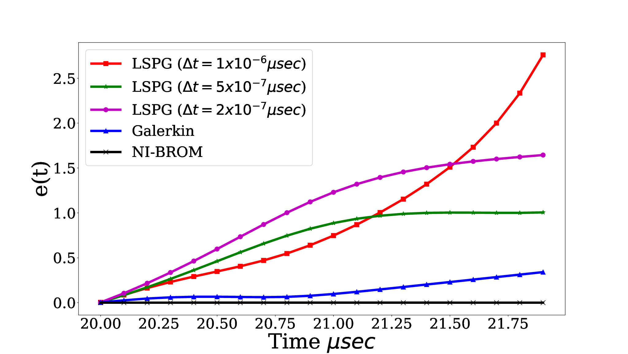
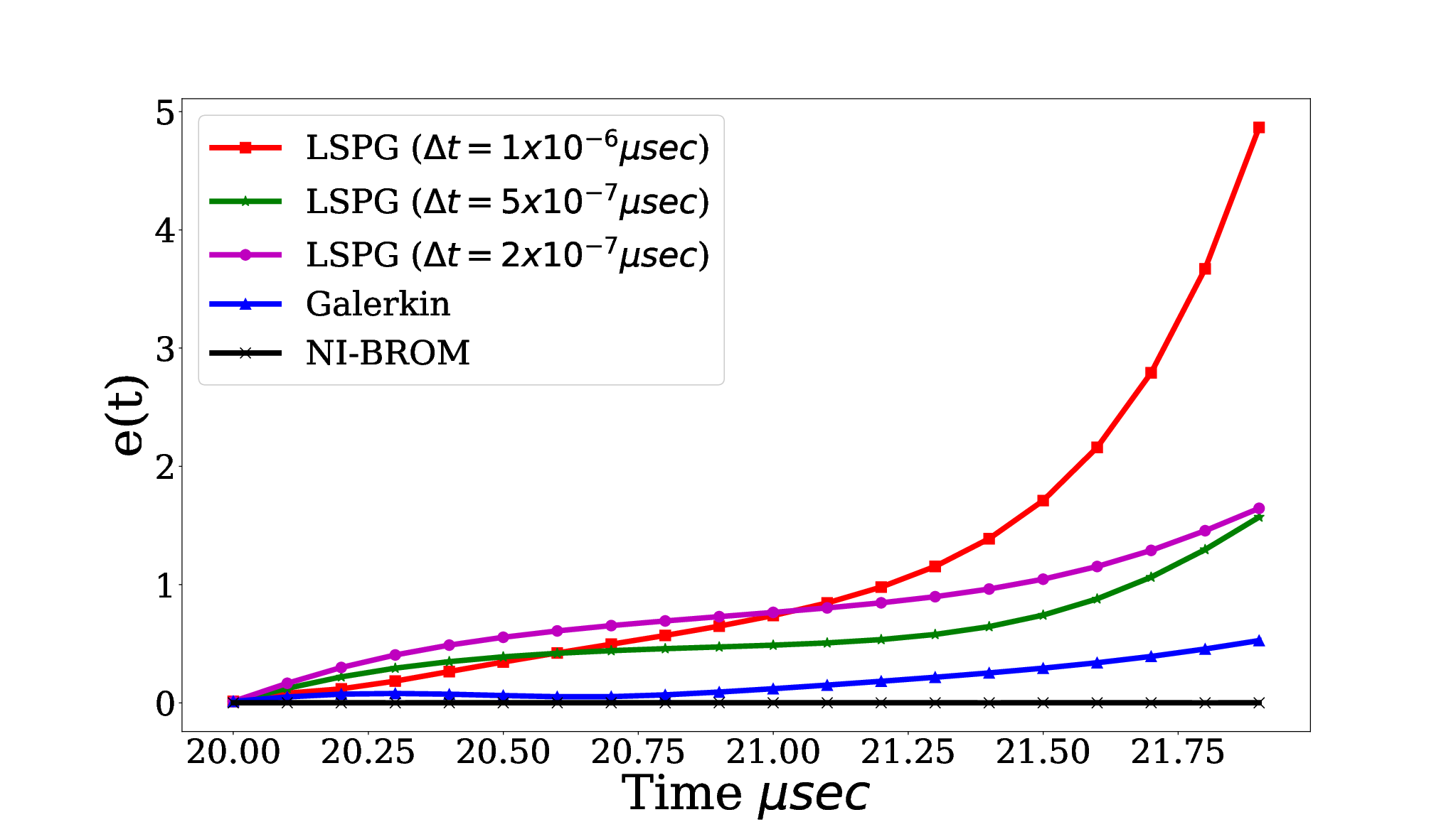
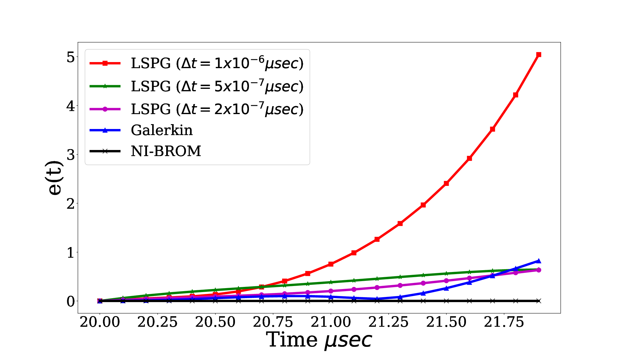
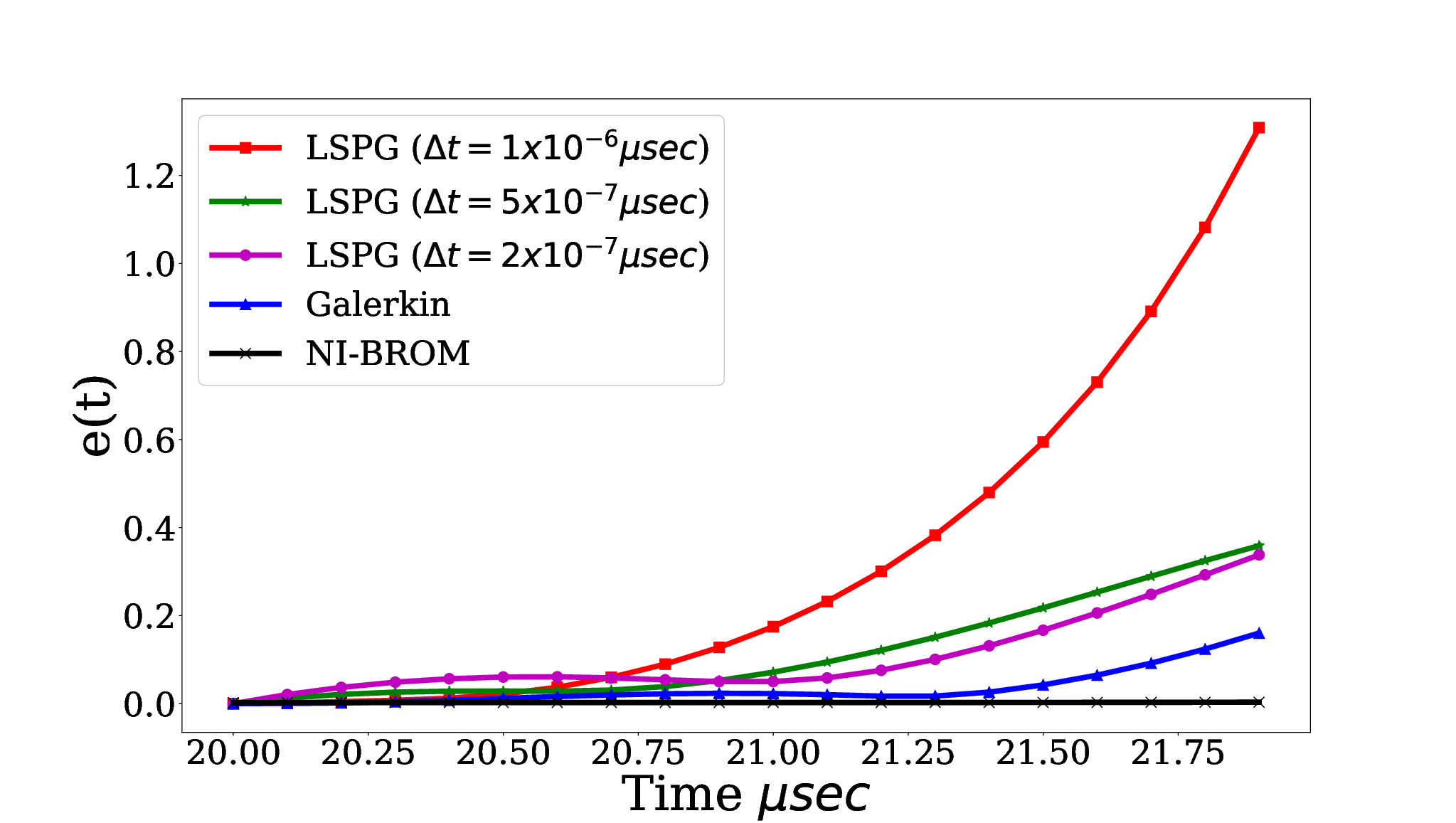
The analysis so far has been based on a perturbation frequency of 215 kHz. Figure 11 demonstrates the predictive performance of balanced ROMs for different perturbation frequencies. The perturbation amplitude is retained at $0.01\%p_{back}$, and the unit impulse response is collected with a sampling period of $T_{s}=0.1\mu sec$ and a total of 1000 Markov parameters are used to train the ROMs. The last 100 cells of the domain are removed from the analysis (after computing the solution and before evaluating the relative errors). As shown in Figure 11 balanced ROM errors decay in time for all frequencies.

Next, we use the output domain decomposition approach with tangential interpolation to resolve the sharp gradients that develop at the vicinity of the right boundary. We have a single-input multi-output (SIMO) system, therefore, reduction is applied only along the left tangential directions. The full-state output is divided into three subdomains (i.e., $q_{m}=3$ in equation (32)), where $\mathbf{C}_{1}\in\mathbb{R}^{950\times 1000}$ corresponds to ROM 1 that is trained with the largest sampling period of $T_{s}=0.1\mu sec$, $\mathbf{C}_{2}\in\mathbb{R}^{45\times 1000}$ corresponds to ROM 2 trained with a sampling period of $T_{s}=0.01\mu sec$, and $\mathbf{C}_{3}\in\mathbb{R}^{5\times 1000}$ is for ROM 3 trained with the smallest sampling period of $T_{s}=0.001\mu sec$. Tangential interpolation is separately applied to ROM 1 and ROM 2. Since ROM 3 originally has a low-dimensional output (state at 5 cells), further reduction of the number of outputs via projection over the tangential directions affects accuracy, therefore, we maintain the original number of outputs in ROM 3. Table 2 lists the wall-clock times of subdomain ROMs with and without tangential interpolation. Projection of the impulse response sequence over the dominant tangential directions has clearly reduced the total offline cost of ERA. It is noted that by a more radical truncation along the left tangential directions ROMs remain stable and offline computations are reduced at the cost of accuracy.

The sensitivity of balanced ROMs constructed with ERA is studied here with respect to the sampling time. As shown in Figure 12, ROMs with 50 and 200 Markov parameters fail to capture the decay of the lightly-damped eigenvector in the impulse response tail and therefore, exhibit a poor predictive performance. Relative prediction error computed for ROMs with 1000 and 2000 Markov parameters overlap. Thus, the impulse response sequence captures the essential dynamics and further increase in the sampling time does not improve accuracy. The relative error profiles in Figure 7 show that the domain decomposition approach has effectively improved accuracy of the balanced ROMs by resolving the numerical errors at the right boundary, despite the impulse response sequence is projected onto a lower-dimensional output space via the tangential interpolation. We have not used domain decomposition for the species mass fraction, since the sharp gradients are only observed in pressure, velocity, and temperature profiles.

We further investigate the sensitivity of the balanced ROMs with respect to sampling properties by evaluating the relative prediction error of ROMs trained with different impulse response sampling frequencies shown in Figure 13. Sampling periods of $T_{s}=1\mu sec$ and $T_{s}=0.5\mu sec$ seem to leave out some of the high-frequency structures that are critical to the dynamics of the system. The error reduces as the sampling period is decreased to $T_{s}=0.1\mu sec$, which showed good agreement with the FOM in Figure 7 for unseen forcing input. Training subdomain ROMs with different sampling periods in the output domain decomposition approach has clearly improved accuracy of the state prediction by one to two orders of magnitude.

References

- [1] Aditya K, Gruber A, Xu C, Lu T, Krisman A, Bothien M, Chen J. 2019 Direct numerical simulation of flame stabilization assisted by autoignition in a reheat gas turbine combustor. Proceedings of the Combustion Institute 37, 2635–2642.
- [2] Elghobashi S. 2020 Direct numerical simulation of turbulent flows laden with droplets or bubbles. Annual Review of Fluid Mechanics 51, 217–244.
- [3] Zhang C, Duan L, Choudhari M. 2018 Direct numerical simulation database for supersonic and hypersonic turbulent boundary layers. AIAA journal 56, 4297–4311.
- [4] Lee M, Moser R. 2015 Direct numerical simulation of turbulent channel flow up to . J Fluid Mech 774, 395–415.
- [5] Noack B, Niven R. 2013 A hierarchy of maximum entropy closures for Galerkin systems of incompressible flows. Comput Math Appl 65, 1558–1574.
- [6] Wei M, Rowley C. 2009 Low-dimensional models of a temporally evolving free shear layer. J Fluid Mech 228, 113–134.
- [7] Wei M, Qawasmeh B, Barone M, van Bloemen Waanders B, Zhou L. 2012 Low-dimensional model of spatial shear layers. Phys Fluids 24, 014108.
- [8] Ohlberger M, Rave S. 2015 Reduced basis methods: Success, limitations and future challenges. arXiv preprint arXiv:1511.02021.
- [9] Holmes P, Lumley J, Berkooz G. 1996 Turbulence, Coherent Structures, Dynamical Systems and Symmetry. New York: Cambridge University Press.
- [10] Berkooz G, Holmes P, Lumley L. 1993 The proper orthogonal decomposition in the analysis of turbulent flows. Ann Rev Fluid Mech 25, 539–575.
- [11] Sirovich L. 1987 Turbulence and the dynamics of coherent structures. Q Appl Math 45, 561–590.
- [12] Rowley C, Colonius T, Murray R. 2004 Model reduction for compressible flows using POD and Galerkin projection. Physica D 189, 115–129.
- [13] Lee K, Carlberg K. 2020 Model reduction of dynamical systems on nonlinear manifolds using deep convolutional autoencoders. J Comp Phys. 404, 108973.
- [14] Ghattas O, Willcox, K. . 2021 Learning physics-based models from data: perspectives from inverse problems and model reduction. Proceedings of the Royal Society A 30, 445–554.
- [15] Benner P, Gugercin S, Willcox K. 2015 A survey of projection-based model reduction methods for parametric dynamical systems. SIAM review 57, 483–531.
- [16] Serre G, Lafon P, Gloerfelt X, Bailly C. 2012 Reliable reduced-order models for time-dependent linearized Euler equations. J Comp Phys 231, 5176–5194.
- [17] Rezaian E, Wei M. 2021 A global eigenvalue reassignment method for the stabilization of nonlinear reduced-order models. Int J Numer Methods Eng 122, 2393–2416.
- [18] Pan S, Duraisamy K. 2018 Data-driven discovery of closure models. SIAM Journal on Applied Dynamical Systems 17, 2381–2413.
- [19] Iliescu T, Wang Z. 2013 Variational multiscale proper orthogonal decomposition: Convection-dominated convection-diffusion-reaction equations. Math Comput 82, 1357–1378.
- [20] Wells D, Wang Z, Xie X, Iliescu T. 2017 An evolve-then-filter regularized reduced order model for convection-dominated flows. Int J Numer Meth Fl 84, 598–615.
- [21] Kalashnikova I, van Bloemen Waanders B, Arunajatesan S, Barone M. 2014 Stabilization of projection-based reduced order models for linear time-invariant systems via optimization-based eigenvalue reassignment. Comput Methods Appl Mech Eng 272, 251–270.
- [22] Rezaian E, Wei M. 2020 A hybrid stabilization approach for reduced-order models of compressible flows with shock-vortex interaction. Int J Numer Methods Eng 121, 1629–1646.
- [23] Mojgani R, Balajewicz M. 2020 Stabilization of linear time-varying reduced order models, a feedback controller approach. Int J Numer Meth Eng 121, 5490–5510.
- [24] Amsallem D, Farhat C. 2012 Stabilization of projection-based reduced-order models. Int J Numer Methods Eng 91, 358–377.
- [25] Balajewicz M, Tezaur I, Dowell E. 2016 Minimal subspace rotation on the Stiefel manifold for stabilization and enhancement of projection-based reduced order models for the compressible Navier-Stokes equations. J Comp Phys 321, 224–241.
- [26] Lucia D, Beran P. 2003 Projection methods for reduced order models of compressible flows. J Comp Phys. 188, 252–280.
- [27] Barone M, Kalashnikova I, Segalman D, Thornquist H. 2009 Stable Galerkin reduced order models for linearized compressible flow. J Comput Phys 228, 1932–1946.
- [28] Kalashnikova I, Barone M. 2011 Stable and efficient Galerkin reduced order models for non-linear fluid flow. 6th AIAA Theoretical Fluid Mechanics Conference p. 3110.
- [29] Chan J. 2020 Entropy stable reduced order modeling of nonlinear conservation laws. J Comput Phys p. 109789.
- [30] Carlberg K, Bou-Mosleh C, Farhat C. 2011 Efficient non-linear model reduction via a least-squares Petrov-Galerkin projection and compressive tensor approximations. Int J Numer Meth Eng 86, 155–181.
- [31] Bui-Thanh T, Willcox K, Ghattas O. 2008 Model reduction for large-scale systems with high-dimensional parametric input space. SIAM J Sci Comput 30, 3270–3288.
- [32] Huang C, Wentland C, Duraisamy K, Merkle C. 2020 Model reduction for multi-scale transport problems using structure-preserving least-squares projections with variable transformation. arXiv preprint arXiv:2011.02072.
- [33] Wang Z, Akhtar I, Borggaard J, Iliescu T. 2012 Proper orthogonal decomposition closure models for turbulent flows: a numerical comparison. Computer Methods in Applied Mechanics and Engineering 237, 10–26.
- [34] Ahmed SE, Pawar S, San O, Rasheed A, Iliescu T, Noack BR. 2021 On closures for reduced order models A spectrum of first-principle to machine-learned avenues. arXiv preprint arXiv:2106.14954.
- [35] Rempfer D, Fasel H. 1994 Dynamics of three-dimensional coherent structures in a flat-plate boundary layer. J Fluid Mech 275, 257–283.
- [36] Gouasmi A, Parish E, Duraisamy K. 2017 A priori estimation of memory effects in reduced-order models of nonlinear systems using the Mori–Zwanzig formalism. Proceedings of the Royal Society A 473, 20170385.
- [37] Parish EJ, Wentland CR, Duraisamy K. 2020 The Adjoint Petrov–Galerkin method for non-linear model reduction. Computer Methods in Applied Mechanics and Engineering 365, 112991.
- [38] Rowley C. 2005 Model reduction for fluids, using balanced Proper Orthogonal Decomposition. Int J Bifurcat Chaos 15, 997–1013.
- [39] Moore B. 1981 Principal component analysis in linear systems: Controllability, observability, and model reduction. IEEE transactions on automatic control 26, 17–32.
- [40] Antoulas A. 2005 Approximation of large-scale dynamical systems. Society for Industrial and Applied Mathematics.
- [41] Vettermann J, Sauerzapf S, Naumann A, Beitelschmidt M, Herzog R, Benner P, Saak J. 2021 Model Order Reduction Methods for Coupled Machine Tool Models. MM Science Journal p. DOI: 10.17973/MMSJ.2021_7_2021072.
- [42] Behr M, Benner P, Heiland J. 2021 Invariant Galerkin Trial Spaces and Davison-Maki Methods for the Numerical Solution of Differential Riccati Equations. p. arXiv:1910.13362.
- [43] Benner P, Breiten T. 2013 Low rank methods for a class of generalized Lyapunov equations and related issues. Numerische Mathematik 124, 441–470.
- [44] Shank S, Simoncini V, Szyld D. 2016 Efficient low-rank solution of generalized Lyapunov equations. Numerische Mathematik 134, 327–342.
- [45] Willcox K, Peraire J. 2002 Balanced model reduction via the proper orthogonal decomposition. AIAA journal 40, 2323–2330.
- [46] Flinois T, Morgans A, Schmid P. 2015 Projection-free approximate balanced truncation of large unstable systems. Physical Review E 92, 023012.
- [47] Juang J. 1994 Applied system identification. Prentice-Hall, Inc.
- [48] Ma Z, Ahuja S, Rowley C. 2011 Reduced-order models for control of fluids using the eigensystem realization algorithm. Theoret Comput Fluid Dyn 25, 233–247.
- [49] Peherstorfer B, Willcox K. 2016 Data-driven operator inference for nonintrusive projection-based model reduction. Computer Methods in Applied Mechanics and Engineering 306, 196–215.
- [50] McQuarrie S, Huang C, Willcox K. 2021 Data-driven reduced-order models via regularised Operator Inference for a single-injector combustion process. Journal of the Royal Society of New Zealand 51, 194–211.
- [51] Gosea I, Gugercin S, Beattie C. 2021 Data-driven balancing of linear dynamical systems. arXiv preprint arXiv:2104.01006.
- [52] Tu J, Rowley C, Luchtenburg D, Brunton S, Kutz J. 2014 On Dynamic Mode Decomposition: Theory and Applications. arXiv:1312.0041.
- [53] Hammarling S. 1982 Numerical solution of the stable, non-negative definite lyapunov equation. IMA Journal of Numerical Analysis 2, 303–323.
- [54] Glover K. 1984 All optimal Hankel-norm approximations of linear multivariable systems and their L,-error bounds. International journal of control 39, 1115–1193.
- [55] Hinrichsen D, Pritchard A. 1990 An improved error estimate for reduced-order models of discrete-time systems. IEEE Transactions on Automatic Control 35, 317–320.
- [56] Kramer B, Gugercin S. 2016 Tangential interpolation-based eigensystem realization algorithm for MIMO systems. Mathematical and Computer Modelling of Dynamical Systems, 22, 282–306.
- [57] Lumley J, Poje A. 1997 Low-dimensional models for flows with density fluctuations. Physics of Fluids 9, 2023–2031.
- [58] Carlberg K, Barone M, Antil H. 2017 Galerkin v. least-squares Petrov–Galerkin projection in nonlinear model reduction. J Comput Phys 330, 693–734.
- [59] Carlberg K. 2015 Adaptive h-refinement for reduced-order models. International Journal for Numerical Methods in Engineering 102, 1192–1210.
- [60] Brunton S, Kutz J. 2019 Data-driven science and engineering: Machine learning, dynamical systems, and control. New York: Cambridge University Press.
- [61] Turns S. 1996 Introduction to combustion. New York: McGraw-Hill Companies.
- [62] Wentland C. 2021 Prototyping Environment for Reacting Flow Order Reduction Methods (PERFORM). https://doi.org/10.5281/zenodo.5517532.
- [63] Tu J, Rowley C. 2012 An improved algorithm for balanced POD through an analytic treatment of impulse response tails. Journal of Computational Physics 231, 5317–5333.