Coalgebra symmetry for discrete systems

Giorgio Gubbiotti Address: Scuola Internazionale Superiore di Studi Avanzati, Via Bonomea 265, 34136 Trieste, Italy Current address: Dipartimento di Matematica “Federigo Enriques”, Università degli Studi di Milano, Via C. Saldini 50, 20133 Milano, Italy Email address: giorgio.gubbiotti@unimi.it , Danilo Latini Address: School of Mathematics and Physics, The University of Queensland, Brisbane, QLD 4072, Australia Email address: d.latini@uq.edu.au and Benjamin K. Tapley Address: Department of Mathematical Sciences, NTNU, 7491 Trondheim, Norway Email address: benjamin.tapley@ntnu.no

Abstract.

In this paper we introduce the notion of coalgebra symmetry for discrete systems. With this concept we prove that all discrete radially symmetric systems in standard form are quasi-integrable and that all variational discrete quasi-radially symmetric systems in standard form are Poincaré–Lyapunov–Nekhoroshev maps of order $N-2$ , where $N$ are the degrees of freedom of the system. We also discuss the integrability properties of several vector systems which are generalisations of well-known one degree of freedom discrete integrable systems, including two $N$ degrees of freedom autonomous discrete Painlevé I equations and an $N$ degrees of freedom McMillan map.

2020 Mathematics Subject Classification

39A36; 16T15; 17B62; 17B63.

1. Introduction

In this paper we show how to use the coalgebra symmetry approach to build invariants for discrete systems. In particular, we consider systems of second order difference equations:

(1.1)

\mathbf{x}_{n+1}=\mathbf{F}\left(\mathbf{x}_{n},\mathbf{x}_{n-1}\right),

where the unknown is a sequence of vectors $\left\{\mathbf{x}_{n}\right\}_{n\in\mathbb{Z}}$ in $\mathbb{R}^{N}$ with $N\in\mathbb{N}$ . Like in the continuous case the coalgebra symmetry approach allows us to extend invariants from symplectic systems with one degree of freedom to symplectic systems with $N$ degrees of freedom, see for instance the review [5].

Besides the general definition, we present some general results on the integrability through the coalgebra symmetry approach of some classes of $N$ degrees of freedom analog of the systems in standard form [58]:

(1.2)

x_{n+1}+x_{n-1}=F\left(x_{n}\right),

where $\left\{x_{n}\right\}_{n\in\mathbb{Z}}$ is the unknown function. Integrable examples include a generalisation of the celebrated McMillan equation [45], one of the first integrable discrete systems ever discovered, and of the autonomous discrete Painleve I equation. We underline that a two-degrees of freedom generalisation of the McMillan equation presented already in [44] by a brute-force computation, and later understood in terms of discrete Garnier systems [59]. On the other hand, up to our knowledge, the generalisations of the autonomous Painlevé I equation we present are new.

The extension of the coalgebra approach to the discrete setting we present is a result that paves the way to a systematic study of the integrability conditions for discrete systems with more than one degree of freedom. Indeed, while almost all discrete systems with one degree of freedom fall into the class of the aforementioned QRT maps, with some notable exceptions [70, 23, 55, 17], there is no general analog description for systems with more degrees of freedom. Partial classification of systems in more than one degree of freedom has been given in [30, 16, 29, 44], usually with the additional condition that the system possesses invariants of a given form, or additional structures such as symplectic structures.

So, in this paper we present an efficient way to build discrete systems with $N$ degrees of freedom from those with one degree of freedom, which is something that is completely missing in the discrete case. This gives a new evidence on how techniques developed in the continuum setting can be extended proficiently to the discrete case. We also show that the access to a very efficient integrability test such as the algebraic entropy [13], makes easier to predict the behaviour of the obtained $N$ -degrees of freedom systems.

The plan of the paper is the following: in Section 2 we recall some general result on the integrability of discrete systems. In Section 3 we give the definition of coalgebra symmetry for discrete Poisson maps. The great part of the construction follows the ideas used in the continuous setting, see [5]. However, the definition we state is slightly different from the one used in the continuous setting. In Section 4 we present some general results on two classes of discrete systems, namely the radially symmetric and the quasi-radially symmetric, show their coalgebraic interpretation, and present explicit examples of it. In Section 5 we discuss two non-linear examples which generalise a well-known integrable system, the autonomous discrete Painlevé I equation. In Section 6 we discuss an $N$ degrees of freedom generalisation of the McMillan map. We show that this generalisation is not integrable, but it is only quasi-integrable, while a particular case is quasi-maximally superintegrable. Finally, in Section 7 we give some conclusions and an outlook on future researches and developments.

2. Discrete systems and integrability

In this section we give a preliminary introduction on the concepts of integrability for finite-dimensional discrete systems we are going to use throughout the paper. Differently from finite-dimensional continuous integrable systems whose history can be traced back to the times of Liouville [41], the integrability of their discrete counterpart is a much more recent subject. The history of such a subject can be traced back from the seminal paper of McMillan [45], where the eponymous map was introduced, and had a great propulsion after the introduction of the celebrated QRT maps [50, 51]. In particular, the theory of symplectic integrable maps was developed in [66, 14, 43]. For a complete overview on the subject we refer to the mentioned papers, the review [32], the book [33], and the introductory material in the thesis [63].

2.1. Invariants and integrability

Before considering the vector difference equations in the form (1.1) we consider the general case: let $\{\mathbf{z}_{n}\}\subset\mathbb{R}^{M}$ be a sequence of vectors, solving the first-order vector difference equation

(2.1)

\mathbf{z}_{n+1}=\mathbf{K}\left(\mathbf{z}_{n}\right),

where $\mathbf{K}=\mathbf{K}(\mathbf{z})$ is a locally analytic function of its arguments. This is what we call an $M$ -dimensional difference equation. An invariant for such an equation is a locally analytic function $I=I(\mathbf{z})$ such that $I(\mathbf{z}_{n+1})=I(\mathbf{z}_{n})$ . In such general case we give the following definition:

Definition 2.1.

The first-order $M$ -dimensional difference equation is algebraically integrable if it admits $M-1$ functionally independent invariants.

In general it is quite difficult to find invariant for difference equations. When the equation is rational and invertible with a rational inverse there is an efficient algorithm we recall in Appendix A.

Definition 2.1 is very general, and works for arbitrary maps. If some additional structure is present, the number of invariants needed for integrability can be lowered. Before proceeding any further, we note that any first order difference equation (2.1) is equivalent to iterate a map of the following form:

(2.2)

T\colon\mathbf{z}\in\mathbb{R}^{M}\mapsto\mathbf{K}(\mathbf{z})\in\mathbb{R}^{M}.

We call this form the map form of a first-order difference equation. Since the iteration of the map is equivalent to go from $n$ to $n+1$ we use the shorthand notation $T\colon n\mapsto n+1$ , to denote the map form of a difference equation.

A special, but relevant case is the one of Poisson maps:

Definition 2.2.

Let us assume we are given an $M$ -dimensional difference equation (2.1) and its map form (2.2). Then:

2.2.1.

A Poisson structure of rank $2r$ is a skew-symmetric matrix $J=J\left(\mathbf{z}_{n}\right)$ of constant rank $2r$ such that the Jacobi identity holds:

(2.3)

\sum_{l=1}^{n}\left(J_{li}\frac{\partial J_{jk}}{\partial z_{n,l-1}}+J_{lj}\frac{\partial J_{ki}}{\partial z_{n,l-1}}+J_{lk}\frac{\partial J_{ij}}{\partial z_{n,l-1}}\right)=0,\quad\forall i,j,k.

2.2.2.

Given a Poisson structure $J=J(\mathbf{z}_{n})$ we define its associated Poisson bracket as:

(2.4) $\{f,g\}=\nabla fJ\left(\mathbf{z}_{n}\right)\nabla g^{T},$

where $f$ , $g$ are locally analytic functions on $\mathbb{R}^{M}$ , and $\nabla$ denotes the gradient operator.
2.2.3.

Two locally analytic functions $f$ and $g$ are said to be in involution with respect to a Poisson structure $J=J\left(\mathbf{z}_{n}\right)$ if $\left\{f,g\right\}=0$ .

2.2.4.

An $M$ -dimensional difference equation is a Poisson map if it preserves the Poisson structure $J\left(\mathbf{z}_{n}\right)$ , i.e.:

(2.5)

\frac{\partial\mathbf{z}_{n+1}}{\partial\mathbf{z}_{n}}J({\mathbf{z}_{n}})\left(\frac{\partial\mathbf{z}_{n+1}}{\partial\mathbf{z}_{n}}\right)^{T}=J({\mathbf{z}_{n+1}}),

where $\partial\mathbf{z}_{n+1}/\partial\mathbf{z}_{n}$ is the Jacobian matrix of $\mathbf{z}_{n+1}$ .

Remark 2.1.

We can easily see that $\{z_{n,i-1},z_{n,j-1}\}=J_{ij}(\mathbf{z}_{n})$ . Since this completely specifies the Poisson structure, it is usual to give it in terms of the commutation relations of the dependent variables $\mathbf{z}_{n}$ .

Then we have the following characterisation of integrability for Poisson maps:

Definition 2.3 ([66, 14, 43]).

An $M$ -dimensional Poisson map $T\colon n\mapsto n+1$ with respect to a Poisson structure of rank $2r$ is Liouville–Poisson integrable if it possesses $M-r$ functionally independent invariants in involution with respect to the associated Poisson bracket.

Remark 2.2.

The rank of a Poisson structure is such that $1\leq r\leq\lfloor M/2\rfloor$ . So we can distinguish two extremal cases:

•

Minimal rank $r=1$ : the number of invariants needed for Liouville–Poisson integrability is maximal, that is $M-1$ . In this case Liouville–Poisson integrability is equivalent to algebraic integrability, see definition 2.1.
•

Maximal rank $r=\lfloor M/2\rfloor$ : the number of invariants needed for Liouville–Poisson integrability is minimal, that is $M-\lfloor M/2\rfloor$ .

A relevant case is when the rank is maximal and the dimension is even, that is $M=2r$ . In such case the Poisson structure is invertible; defining $\Omega=J^{-1}$ we call such a matrix a symplectic structure, and a map preserving it is a symplectic map. In the full rank case the number of invariants needed is exactly half of the dimension of the base space $M/2$ . In such a case the number $N:=M/2$ is called the number of degrees of freedom of the system.

The previous remark highlight a very special case of Liouville–Poisson integrability, which we state as a separate definition:

Definition 2.4 ([66, 14, 43]).

An $2N$ -dimensional ( $N$ degrees of freedom) symplectic map $T\colon n\mapsto n+1$ is Liouville integrable if it possesses $N$ functionally independent invariants in involution with respect to the associated Poisson bracket.

Furthermore, we give some additional definition to cover the cases when there exist more or less invariants than the number given in Definitions 2.1 and 2.3.

Definition 2.5.

Suppose we are given a Poisson map $T\colon n\mapsto n+1$ (2.2), with associated Poisson structure of rank $2r$ . Then:

2.5.1.
If $T\colon n\mapsto n+1$ is Liouville–Poisson integrable, and possesses $k$ additional functionally independent invariants, with $0<k<r$ , then it is said to be superintegrable. Moreover:
1. 2.5.1.a.
  
  if $k=1$ the map is said to be minimally superintegrable,
2. 2.5.1.b.
  
  if $k=r-2$ the map is said to be quasi-maximally superintegrable,
3. 2.5.1.c.
  
  if $k=r-1$ the map is said to be maximally superintegrable.
2.5.2.
If $T\colon n\mapsto n+1$ possesses $\kappa$ commuting functionally independent invariants with $0<\kappa<M-r$ , then it is said to be Poincaré–Lyapunov–Nekhoroshev (PLN) map of order $\kappa$ . Moreover:
1. 2.5.2.a.
  
  if $\kappa=1$ the map is said to be Poincaré–Lyapunov (PL) map,
2. 2.5.2.b.
  
  if $\kappa=M-r-1$ the map is said to be quasi-integrable,

Remark 2.3.

We make the following observations:

•

In the literature on superintegrable systems, see for instance [46], it is often omitted in the definition of superingrability the requirement for the system to be Liouville–Poisson integrable. In fact there are known examples in the literature where it is possible to find a huge number of invariants, but not a full set of commuting ones, see [6]. So, to avoid the situation where a superintegrable system might not be a Liouville–Poisson integrable systems, we prefer to stick to a definition where superintegrability requires Liouville–Poisson integrability. We will see an example of discrete system with such a property in Section 6.
•
In the symplectic case ( $M=2N$ ) a symplectic map is:
- –
  
  superintegrable when it is Liouville integrable and possesses $N<k<2N$ invariants,
- –
  
  quasi-maximally superintegrable when it is superintegrable and possesses $2N-2$ invariants,
- –
  
  maximally superintegrable when it is superintegrable and possesses $2N-1$ invariants.
- –
  
  quasi-integrable when it possesses $N-1$ commuting invariants.

2.2. Variational discrete systems and their integrability

Given a $M$ -dimensional difference equation (2.1), it is not easy to decide if there exists a compatible Poisson or symplectic structure. Some partial results were given in [15]. An important particular case is when the equation is variational, that is when the system arises from a discrete Lagrangian, see [42, 66, 14, 64, 28] for further details. In particular we also mention that the relationship of variational structures with Liouville integrability was used in [30, 29] to prove integrability of some four-dimensional difference equations.

Let us stick to our case of interest: a system of second-order difference equations of the form (1.1) is variational if there exist a function

(2.6)

L=L_{n}(\mathbf{x}_{n+1},\mathbf{x}_{n}),

called the discrete Lagrangian, such that the system itself is equivalent to the Euler-Lagrange equations:

(2.7)

\nabla_{\mathbf{x}_{n}}\left[L_{n}(\mathbf{x}_{n+1},\mathbf{x}_{n})+L_{n-1}(\mathbf{x}_{n},\mathbf{x}_{n-1})\right]=0.

Note that in general the Euler–Lagrange equations are a multi-valued function in $\mathbf{x}_{n+1}$ and $\mathbf{x}_{n-1}$ , see [33]. Then we have the following result:

Lemma 2.1 ([14, 33]).

If the discrete Lagrangian $L$ does not depend explicitly on $n$ , then the Euler–Lagrange equations (2.7) leave invariant the following symplectic structure:

(2.8)

\Omega(\mathbf{x}_{n},\mathbf{x}_{n-1})=\begin{pmatrix}\mathbb{O}_{N}&\Lambda_{N}(\mathbf{x}_{n},\mathbf{x}_{n-1})\\ -\Lambda_{N}(\mathbf{x}_{n},\mathbf{x}_{n-1})&\mathbb{O}_{N}\end{pmatrix}

where $\mathbb{O}_{N}$ is the zero $N\times N$ matrix and:

(2.9)

\Lambda_{N}(\mathbf{x}_{n},\mathbf{x}_{n-1})=\begin{pmatrix}\dfrac{\partial^{2}L}{\partial x_{n,1}\partial x_{n-1,1}}&\dots&\dfrac{\partial^{2}L}{\partial x_{n,1}\partial x_{n-1,N}}\\[8.61108pt] \vdots&&\vdots\\[8.61108pt] \dfrac{\partial^{2}L}{\partial x_{n,N}\partial x_{n-1,1}}&\dots&\dfrac{\partial^{2}L}{\partial x_{n,N}\partial x_{n-1,N}}\end{pmatrix}.

For generalisations and proof of such a result we refer to [63].

3. Coalgebra symmetry for discrete systems

The coalgebra symmetry approach to (super)integrable systems is an approach that allows to build a (classical) Liouville integrable system on the tensor product of $N$ copies of a given Poisson algebra $\mathfrak{A}$ . The concept of coalgebra originated in Quantum Group theory and it was not until the papers [12, 7] that its application to (classical) Liouville integrable was devised. We note that besides these seminal applications the coalgebra symmetry approach has been extended to many other cases, and many integrable and superintegrable systems have been understood within this algebraic framework. For a comprehensive review containing several explicit examples (for deformed coalgebras also), some generalisations of the method (such as comodule algebras [3] and Loop coproducts [48]) and many references on the topic we refer the reader to [5]. Additional examples, where other physical applications can be found (also in the quantum mechanical setting), involve superintegrable systems defined on non-Euclidean spaces [2, 8, 9, 11, 10, 53, 49], models with spin-orbital interactions [54], discrete quantum mechanical systems [40] and superintegrable systems related to the generalised Racah algebra $R(n)$ [21, 37, 38, 39].

Roughly speaking, the general idea behind this algebraic approach is to reinterpret one degrees of freedom dynamical Hamiltonian systems as the images, under a given symplectic realisation, of some (smooth) functions of the generators of a given Poisson (co)algebra $(\mathfrak{A},\Delta)$ . Then, by using the (not necessarily primitive) coproduct, the method consists in extending the one degrees of freedom system, originally defined on $\mathfrak{A}$ , to a higher degrees of freedom one defined on the tensor product of $N$ copies of $\mathfrak{A}$ . The main point resides in the fact that the obtained higher degrees of freedom system is endowed with constants of motion arising as the images of the coalgebra Casimir invariants through the application of the so-called $m$ th coproduct maps. In this section, we will recall the definition of coalgebra and then adapt it to the study of (super)integrable discrete systems.

3.1. Definition of coalgebra and coproduct

We state the following main definition:

Definition 3.1 ([19, 22]).

A coalgebra is a pair of objects $(\mathfrak{A},\Delta)$ where $\mathfrak{A}$ is a unital, associative algebra and $\Delta\colon\mathfrak{A}\rightarrow\mathfrak{A}\otimes\mathfrak{A}$ is a coassociative map, that is:

(3.1)

(\Delta\otimes\Id)\circ\Delta=(\Id\otimes\Delta)\circ\Delta.

meaning that the following diagram is commutative:

(3.2)

\begin{CD}\mathfrak{A}@>{\Delta}>{}>\mathfrak{A}\otimes\mathfrak{A}\\ @V{\Delta}V{}V@V{}V{\Delta\otimes\Id}V\\ \mathfrak{A}\otimes\mathfrak{A}@>{}>{\Id\otimes\Delta}>\mathfrak{A}\otimes\mathfrak{A}\otimes\mathfrak{A}\end{CD}

and is an algebra homomorphism from $\mathfrak{A}$ to $\mathfrak{A}\otimes\mathfrak{A}$ , i.e. $\Delta(X\cdot Y)=\Delta(X)\cdot\Delta(Y)$ , for all $X,Y\in\mathfrak{A}$ . The map $\Delta$ is called the coproduct map.

As for Definition 3.1 the base algebra $\mathfrak{A}$ of a coalgebra $(\mathfrak{A},\Delta)$ can be any unital algebra. However, following [7] we are interested to the case when the algebra $\mathfrak{A}$ is a Poisson algebra. We have then the following definition:

Definition 3.2.

The pair $(\mathfrak{A},\Delta)$ is a Poisson coalgebra if $\mathfrak{A}$ is a Poisson algebra and $\Delta$ is a Poisson homomorphism between $\mathfrak{A}$ and $\mathfrak{A}\otimes\mathfrak{A}$ , i.e.:

(3.3)

\Delta\bigl(\{X,Y\}_{\mathfrak{A}}\bigl)=\{\Delta(X),\Delta(Y)\}_{\mathfrak{A}\otimes\mathfrak{A}}\quad\forall\,X,Y\in\mathfrak{A}\,,

with respect to the standard Poisson structure on $\mathfrak{A}\otimes\mathfrak{A}$ given by:

(3.4)

\{X\otimes Y,W\otimes Z\}_{\mathfrak{A}\otimes\mathfrak{A}}:=\{X,W\}_{\mathfrak{A}}\otimes YZ+XW\otimes\{Y,Z\}_{\mathfrak{A}},

for all $X,Y,Z,W\in\mathfrak{A}$ .

So, let $(\mathfrak{A},\Delta)$ be a Poisson coalgebra generated by the set $\left\{A_{1},\dots,A_{K}\right\}$ , with $K:=\text{dim}(\mathfrak{A})$ . In what follows we will denote by $C_{i}=C_{i}\left(A_{1},\dots,A_{K}\right)$ for $i=1,\dots,r$ the $r$ functionally independent Casimir functions of $\mathfrak{A}$ .

Remark 3.1.

We remark that also when $\mathfrak{A}$ is a Poisson algebra, the definition of the coproduct map might be non-trivial. However, for Lie–Poisson algebras with generators $A_{i}$ , $i=1,\dots,K$ , the coproduct is primitive [62], i.e.:

(3.5)

\Delta(A_{i})=A_{i}\otimes 1+1\otimes A_{i}\qquad\Delta(1)=1\otimes 1,

and for general elements it is defined by extension.

By recursion we can define the $m$ th coproduct $\Delta^{(m)}\colon\mathfrak{A}\rightarrow\mathfrak{A}^{\otimes m}$ , where $\mathfrak{A}^{\otimes m}=\bigotimes_{i=1}^{m}\mathfrak{A}$ , as:

(3.6)

\Delta^{(m)}:=\begin{cases}\Delta&\text{if $m=2$},\\ \bigl(\overbrace{\Id\otimes\Id\otimes\dots\otimes\Id}^{m-2}\otimes\Delta^{(2)}\bigr)\circ\Delta^{(m-1)}.&\text{if $m>2$}.\end{cases}

By induction on $m$ , from the fact that $\Delta$ is a Poisson map on $\mathfrak{A}\otimes\mathfrak{A}$ we have that the $m$ th coproduct $\Delta^{(m)}$ is a Poisson map on $\mathfrak{A}^{\otimes m}$ [7, 5] (see also [48]).

Using the $m$ th coproduct it is possible to define elements on $\mathfrak{A}^{\otimes m}$ by applying it to the generators $A_{i}$ of the original Poisson algebra $\mathfrak{A}$ . This can be extended to functions $h\in\mathcal{C}^{\infty}(\mathfrak{A})$ through the following formula:

(3.7)

h^{(m)}:=\Delta^{(m)}(h)(A_{1},\dots,A_{K}):=h(\Delta^{(m)}(A_{1}),\dots,\Delta^{(m)}(A_{K})).

Clearly $h^{(m)}\in\mathcal{C}^{\infty}(\mathfrak{A}^{\otimes m})$ .

3.2. Coalgebra symmetry and Liouville integrability

The extension we just proposed can be performed to the Casimir elements to produce a set of commuting invariants on a given realisation in $N$ degrees of freedom. This is the first link of the coalgebra structure with Liouville integrability.

To be more specific, let us take a $N\in\mathbb{N}$ fixed. Then we can consider a chain of tensor products $\mathfrak{A}^{\otimes m}$ for all $m\leq N$ with embedding:

(3.8)

j_{m}\colon A\in\mathfrak{A}^{\otimes m}\mapsto A\otimes\overbrace{1\otimes 1\otimes\dots\otimes 1}^{N-m}\in\mathfrak{A}^{\otimes N},

so that we can consider all the elements as lying in the final tensor product $\mathfrak{A}^{\otimes N}$ . In particular, see [47], we can consider all the Poisson brackets in $\mathfrak{A}^{\otimes N}$ in the following way: let $A\in\mathfrak{A}^{\otimes m}$ and $A^{\prime}\in\mathfrak{A}^{\otimes m^{\prime}}$ , then:

(3.9)

\left\{A,A^{\prime}\right\}_{\mathfrak{A}^{\otimes N}}=\left\{j_{m}(A),j_{m^{\prime}}(A^{\prime})\right\}_{\mathfrak{A}^{\otimes N}}.

We state the following:

Lemma 3.1 ([7]).

Consider the following $rN$ functions:

(3.10)

\mathcal{F}_{m,j}:=\Delta^{(m)}(C_{j})(A_{1},\dots,A_{K}),\quad m=1,\dots,N,j=1,\dots,r.

Then the set $\mathcal{L}_{\mathsf{r},N}=\left\{\mathcal{F}_{m,j}\right\}_{m=1,\dots,N,j=1,\dots,r}$ is a set of Poisson-commuting functions on $\mathfrak{A}^{\otimes N}$ . Furthermore, they Poisson commute with $\Delta^{(N)}(A_{i})$ , $i=1,\dots,K$ .

Proof.

We refer the reader to [7, 5]. ∎

In the continuum case, one can use formula (3.7) to define a $N$ -degrees of freedom Hamiltonian starting from a one degree of freedom Hamiltonian. That is, taking a function $h\in\mathcal{C}^{\infty}(\mathfrak{A})$ , we generate its $N$ degrees of freedom extension by defining $h^{(N)}\in\mathcal{C}^{\infty}(\mathfrak{A}^{\otimes N})$ from equation (3.7). A Hamiltonian constructed in this way is said to admit the coalgebra symmetry, and by taking into account Lemma 3.1, it is possible to show that Poisson commutes with the functions $\mathcal{F}_{m,j}$ making them invariants (first integrals) of the associated dynamical system of Hamilton equations [7, 5].

As underlined in the previous section, in the discrete setting there is no exact discrete analog of the Hamiltonian, so the construction we just explained does not extend trivially. However, we consider the evolution of the generator of the Poisson algebra $\mathfrak{A}$ under the flow of a discrete dynamical system. In such a case to underline the discrete nature of the evolution we specify the Poisson algebra as $\mathfrak{A}=\langle A_{1}^{(n)},\dots,A_{K}^{(n)}\rangle$ , and work with a given symplectic realisation of $\mathfrak{A}$ . We then state the following definition:

Definition 3.3.

A Poisson map $T\colon n\mapsto n+1$ is said to possess the coalgebra symmetry with respect to the Poisson coalgebra $(\mathfrak{A},\Delta)$ if for all $N\in\mathbb{N}$ the evolution of generators in a fixed symplectic realisation in $N$ degrees of freedom of the Poisson coalgebra is:

(i)

closed in the Poisson coalgebra, that is:

(3.11) $A_{i}^{(n+1)}=a_{i}(A_{1}^{(n)},\dots,A_{K}^{(n)}),\quad i=1,\dots,K,$

with $a_{i}\in\mathcal{C}^{\infty}(\mathfrak{A})$ ,
(ii)

it is a Poisson map with respect to the Poisson algebra $\mathfrak{A}$ , that is:

(3.12) $\{A_{i}^{(n+1)},A_{j}^{(n+1)}\}=T\bigl(\{A_{i}^{(n)},A_{j}^{(n)}\}\bigr),\quad i,j=1,\dots,K,$
(iii)

admits the Casimirs $\{C_{1}^{(n)},\dots,C_{r}^{(n)}\}$ of the algebra $\mathfrak{A}$ as invariants.

So, now note immediately that any invariant for the system (3.11) is an invariant for the original Poisson map. This trivially follows noticing that the system (3.11) on $N$ degrees of freedom symplectic realisation of $\mathfrak{A}$ is a consequence of the Poisson map itself: using the coordinate realisation we are able to build the invariants in the original coordinates. This construction, enables us to summarise our construction of the discrete coalgebra symmetry in the following theorem:

Theorem 3.2.

Consider a Poisson map $T\colon n\mapsto n+1$ with coalgebra symmetry with respect to the coalgebra $(\mathfrak{A},\Delta)$ . Then $T\colon n\mapsto n+1$ admits a set of $rN$ commuting invariants $\mathcal{L}_{r,N}$ (3.10).

Proof.

The proof follows trivially applying the $m$ th coproduct to the system (3.11), and then considering the construction of the functions $\mathcal{F}_{j,m}$ (3.10). Commutation follows from Lemma 3.1. ∎

3.3. Coalgebra symmetry and superintegrability

In what we discussed in the previous sections we applied recursively the map $\Delta^{(2)}$ to define the $m$ -th coproduct maps $\Delta^{(m)}$ . However, besides (3.6) another recursive relation can be defined for the $m$ -th coproduct maps, i.e. [5]:

(3.13)

\Delta^{(m)}_{R}:=\begin{cases}\Delta&\text{if $m=2$},\\ \bigl(\Delta^{(2)}\otimes\overbrace{\Id\otimes\Id\otimes\dots\otimes\Id}^{m-2}\bigr)\circ\Delta^{(m-1)}.&\text{if $2<m\leq N$}.\end{cases}

Since the coproduct is coassociative, we have that for all $N\in\mathbb{N}$ fixed:

(3.14)

\Delta^{(N)}(A_{i})=\Delta_{R}^{(N)}(A_{i}).

However, when lower dimensional coproducts are considered, substantial differences arise. In particular, lower dimensional left $m$ -th coproducts with $2<m<N$ will contain objects living on the tensor product space $1\otimes 2\otimes\dots\otimes m$ , whereas lower dimensional right $m$ -th coproducts will be defined on the sites $(N-m+1)\otimes(N-m+2)\otimes\dots\otimes N$ . This implies that coalgebra symmetry not only generate a completely integrable Hamiltonian system but, in principle, a superintegrable one. This is because besides the left Casimirs (3.10) we will also be able to define the set $\mathcal{R}_{r,N}=\{\mathcal{G}_{m,j}\}_{m=1,\dots,N,j=1,\dots,r}$ composed by the functions

(3.15)

\mathcal{G}_{m,j}:=\Delta^{(m)}_{R}(C_{j})(A_{1},\dots,A_{K}),\quad m=1,\dots,N,j=1,\dots,r.

called the right Casimirs. Analogously than Lemma 3.1 we have that this set is composed by $rN$ functions in involution. Notice that because of the coassociativity property $\mathcal{F}_{N,j}=\mathcal{G}_{N,j}$ , $j=1,\dots r$ .

Summing up we obtain the following result:

Theorem 3.3.

Consider a Poisson map $T\colon n\mapsto n+1$ with coalgebra symmetry with respect to the coalgebra $(\mathfrak{A},\Delta)$ . Then $T\colon n\mapsto n+1$ admits two set of $rN$ commuting invariants: $\mathcal{L}_{r,N}$ (3.10) and $\mathcal{R}_{r,N}$ (3.15).

Remark 3.2.

We remark that the elements of the sets $\mathcal{L}_{r,N}$ and $\mathcal{R}_{r,N}$ in general do not commute between themselves, see for instance [39] for the example of the $\mathfrak{sl}_{2}(\mathbb{R})$ Lie–Poisson algebra.

3.4. Final remarks on the coalgebra symmetry

Before discussing some concrete cases with explicit Lie–Poisson algebras we give some final remarks on the procedure:

(1)

Even in the continuum case it is not possible to tell a priori if a system with coalgebra symmetry is Liouville integrable, see [4]. This depends on the explicit symplectic realisation of the coalgebra $(\mathfrak{A},\Delta)$ chosen and the number of functionally independent invariants that is possible to extract from the set $\mathcal{L}_{r,N}$ . When we have $N$ degrees of freedom it is enough that the set $\mathcal{L}_{r,N}$ consists of $N-1$ functionally independent invariants: the coalgebraic Hamiltonian $h^{(N)}$ will yield the last one.
(2)

In all the examples we will present, even though the set $\mathcal{L}_{r,N}$ consists of $N-1$ functionally independent invariants, it will not be enough to give integrability because of the lack of the Hamiltonian. However, in most cases the additional missing invariants can be found directly studying the system (3.11) with the methods discussed in Appendix A.

4. General classes of additive differential systems and coalgebra

Consider the following system of second-order additive difference equations:

(4.1)

\mathbf{x}_{n+1}+\mathbf{x}_{n-1}=\mathbf{F}\left(\mathbf{x}_{n}\right).

This system preserves the canonical $\mathbb{R}^{2N}$ measure:

(4.2)

m=\ud\mathbf{x}_{n}\wedge\ud\mathbf{x}_{n-1}.

The system (4.1) is not Lagrangian for all choices of the vector function $\mathbf{F}\left(\mathbf{x}_{n}\right)$ . We note that, if there exists a scalar function $V=V(\mathbf{x}_{n})$ such that $\gradient V(\mathbf{x}_{n})=\mathbf{F}(\mathbf{x}_{n})$ , then the system (4.1) can be derived by the following Lagrangian:

(4.3)

L=\mathbf{x}_{n+1}\cdot\mathbf{x}_{n}-V\left(\mathbf{x}_{n}\right).

From Lemma 2.9 we have that to the Lagrangian (4.3) corresponds the canonical (full-rank) Poisson bracket:

(4.4)

\left\{x_{n,i},x_{n,j}\right\}=\left\{x_{n-1,i},x_{n-1,j}\right\}=0,\quad\left\{x_{n,i},x_{n-1,j}\right\}=\delta_{i,j}

where $\delta_{i,j}$ is Kronecker delta.

We now pass to consider two particular cases of systems in the form (4.1) and prove that they possess the coalgebra symmetry.

4.1. Radially symmetric systems and the $\mathfrak{sl}_{2}(\mathbb{R})$ algebra

Consider the following particular case of (4.1):

(4.5)

\mathbf{x}_{n+1}+\mathbf{x}_{n-1}=f\left(\absolutevalue{\vec{x}_{n}}\right)\frac{\mathbf{x}_{n}}{\absolutevalue{\vec{x}_{n}}}.

This system has radial symmetry: if $\mathbf{x}_{n}$ is a solution of (4.5) then $\mathbf{X}_{n}=R\mathbf{x}_{n}$ with $R\in\SO\left(N\right)$ is another solution. The system (4.5) is variational with the following Lagrangian:

(4.6)

L=\mathbf{x}_{n+1}\cdot\mathbf{x}_{n}-V\left(\absolutevalue{\vec{x}_{n}}\right),\quad V\left(r\right)=\int f\left(r\right)\ud r.

From the general case we have that equation (4.5) preserves the canonical Poisson bracket (4.4).

The following result follows from a trivial computation:

Lemma 4.1.

A radially symmetric system (4.5) possesses the following $N\left(N-1\right)/2$ invariants:

(4.7)

L_{i,j}^{(n)}=x_{n,i}x_{n-1,j}-x_{n-1,i}x_{n,j}.

In total there are $2N-3$ functionally independent functions in formula (4.7).

The skewsymmetric invariants $L_{i,j}$ are the discrete analogue of the components of the angular momentum. It is well known that out of the $2N-3$ functionally independent invariant it is possible to construct $N-1$ functionally independent and commuting with respect to the Poisson bracket (4.4). We show how to construct this set of $N-1$ commuting invariants with the coalgebra symmetry approach, as it was proved in the in the continuum case in [6, 5]. This is the content of the following proposition:

Proposition 4.2.

A radially symmetric system (4.5) possesses coalgebra symmetry with respect to the Lie algebra $\mathfrak{sl}_{2}(\mathbb{R})$ with the following $N$ degrees of freedom symplectic realisation:

(4.8)

J_{+}^{(n)}=\mathbf{x}_{n}^{2},\quad J_{-}^{(n)}=\mathbf{x}_{n-1}^{2},\quad J_{3}^{(n)}=\mathbf{x}_{n}\cdot\mathbf{x}_{n-1}.

Remark 4.1.

The commutation relations of the Lie-Poisson algebra $\mathfrak{sl}_{2}(\mathbb{R})$ are (for sake of simplicity when dealing with abstract properties we omit the superscript $(n)$ ):

(4.9)

\{J_{+},J_{-}\}=4J_{3},\quad\{J_{+},J_{3}\}=2J_{+},\quad\{J_{-},J_{3}\}=-2J_{-}.

This algebra has a single Casimir given by

(4.10)

C=J_{+}J_{-}-J_{3}^{2}.

Proof.

We have to prove that the three conditions of Definition 3.3 hold. This can be done by direct computation. For instance, using the explicit form of the recurrence (4.5) we prove that the action on the generators of the $\mathfrak{sl}_{2}(\mathbb{R})$ algebra (4.8) form the following dynamical system:


(4.11a)	$\displaystyle J_{+}^{(n+1)}$	$\displaystyle=f^{2}(\sqrt{J_{+}^{(n)}})-2J_{3}^{(n)}\frac{f(\sqrt{J_{+}^{(n)}})}{\sqrt{J_{+}^{(n)}}}+J_{-}^{(n)},$
(4.11b)	$\displaystyle J_{-}^{(n+1)}$	$\displaystyle=J_{+}^{(n)},$
(4.11c)	$\displaystyle J_{3}^{(n+1)}$	$\displaystyle=-J_{3}^{(n)}+\sqrt{J_{+}^{(n)}}f(\sqrt{J_{+}^{(n)}}).$

Then using the commutation relations (4.9) we prove that they are preserved (see also formula (2.5)). Finally, it is trivial to see that the Casimir function (4.10) is preserved by the evolution (4.11). ∎

So, following the procedure outlined in Section 3, and using the same reasoning in [6, 5], from the left and right Casimir functions of such an algebra we derive the following two sets of functionally-independent invariants commuting with respect to the canonical Poisson bracket (4.4):


(4.12a)	$\displaystyle\mathcal{C}_{m}^{(n)}$	$\displaystyle=\sum_{1\leq i<j\leq m}\left(L_{i,j}^{(n)}\right)^{2},\quad m=2,\dots,N,$
(4.12b)	$\displaystyle\mathcal{D}_{m}^{(n)}$	$\displaystyle=\sum_{N-m+1\leq i<j\leq N}\left(L_{i,j}^{(n)}\right)^{2},\quad m=2,\dots,N.$

Notice that $\mathcal{C}_{N}^{(n)}=J_{+}^{(n)}J_{-}^{(n)}-(J_{3}^{(n)})^{2}=\mathcal{D}_{N}^{(n)}$ because of the coassociativity. This can be summarised in the following theorem:

Theorem 4.3.

A radially symmetric system (4.5) is quasi-integrable with one of the sets of invariants:

(4.13)

\mathcal{L}=\bigl\{\mathcal{C}_{2}^{(n)},\dots,\mathcal{C}_{N}^{(n)}\bigr\}\quad\text{or}\quad\mathcal{R}=\bigl\{\mathcal{D}_{2}^{(n)},\dots,\mathcal{D}_{N}^{(n)}\bigr\},

Additionally, if we can find an additional invariant commuting either with $\mathcal{L}$ or $\mathcal{R}$ , then system becomes Liouville integrable and moreover quasi-maximally superintegrable.

As we noted in Section 3, the invariants of the system (4.11) are invariants of the radially symmetric system (4.5). So, for a given function $f$ studying the system (4.11) we can find the $N$ th invariant mentioned in Theorem 4.3. We now give an explicit example of this occurrence.

Example 1.

Consider the following linear system:

(4.14)

\mathbf{x}_{n+1}+\mathbf{x}_{n-1}=\alpha\mathbf{x}_{n}.

This system is radial with $f\left(\rho\right)=\alpha\rho$ (hence it is variational), and the associated dynamical system (4.11) is:

(4.15)

\begin{gathered}J_{+}^{(n+1)}=\alpha^{2}J_{+}^{(n)}-2\alpha J_{3}^{(n)}+J_{-}^{(n)},\\ J_{-}^{(n+1)}=J_{+}^{(n)},\quad J_{3}^{(n+1)}=-J_{3}^{(n)}+\alpha J_{+}^{(n)}.\end{gathered}

This system is linear and we find the invariant:

(4.16)

\mathcal{H}^{(n)}=J_{+}^{(n)}-\alpha J_{3}^{(n)}+J_{-}^{(n)}.

From Theorem 4.3 we consider the set of invariants:

(4.17)

\mathcal{S}=\left\{\mathcal{H}^{(n)},\mathcal{C}_{2}^{(n)},\dots,\mathcal{C}_{N}^{(n)}\right\}.

Functional independence and involutivity in this set can be proved by induction. So, we proved that the linear system (4.14) is Liouville integrable. Moreover, since there are $2N-3$ functionally independent elements of the discrete angular momentum that are invariants, we have that the system (4.14) is quasi-maximally superintegrable. $\square$

Remark 4.2.

We remark that, with respect to the rank 2 Lie–Poisson bracket (4.9) the system (4.15) is Poisson–Liouville integrable. Indeed, it possesses the Casimir (4.10), and one invariant (4.16).

Remark 4.3.

The linear system (4.14) is actually maximally superintegrable. Indeed it possesses the following invariants:

(4.18)

\mathcal{H}^{(n)}_{k}=x_{n,k}^{2}-\alpha x_{n,k}x_{n-1,k}+x_{n-1,k}^{2},\quad k=1,\dots,N.

The set

(4.19)

\mathcal{S}^{\prime}=\left\{\mathcal{H}^{(n)}_{1},\dots,\mathcal{H}^{(n)}_{N},\mathcal{C}_{2}^{(n)},\dots,\mathcal{C}_{N}^{(n)}\right\}.

is a set of $2N-1$ functionally independent and commuting invariants. This is easily seen by induction because the invariants are polynomial and they all depend on different $x_{n,k}$ . Indeed, the system is a discrete analog of an isotropic harmonic oscillator, which is a well known maximally superintegrable system.

4.2. Quasi-radially symmetric systems and the $h_{6}$ algebra

Consider the following system that is a particular case of (4.1):

(4.20)

\mathbf{x}_{n+1}+\mathbf{x}_{n-1}=f\left(\absolutevalue{\vec{x}_{n}}\right)\frac{\mathbf{x}_{n}}{\absolutevalue{\vec{x}_{n}}}+g\left(\mathbf{x}_{n}\right)\boldsymbol{\beta},

where $g$ is a scalar function and $\boldsymbol{\beta}$ is a constant vector. Since when $g\equiv 0$ equation (4.20) reduces to (4.5) we call such a system of difference equations a quasi-radially symmetric system.

The following result follows from a trivial computation:

Lemma 4.4.

A quasi-radially symmetric system of the form (4.20) possess the following $N\left(N-1\right)\left(N-2\right)/6$ invariants:

(4.21)

K^{(n)}_{i,j,k}=\beta_{i}L_{j,k}^{(n)}+\beta_{j}L_{k,i}^{(n)}+\beta_{k}L_{i,j}^{(n)},\quad 1\leq i<j<k\leq N.

In total there are $2N-5$ functionally independent functions in formula (4.21).

Quasi-radial systems are not always variational. We give the following characterisation (whose proof follows from direct computations):

Lemma 4.5.

A quasi-radially symmetric system (4.20) preserves the canonical Poisson bracket (4.4) if and only if the $g\left(\mathbf{x}_{n}\right)\equiv h\left(\boldsymbol{\beta}\cdot\mathbf{x}_{n}\right)$ , that is:

(4.22)

\mathbf{x}_{n+1}+\mathbf{x}_{n-1}=f\left(\absolutevalue{\vec{x}_{n}}\right)\frac{\mathbf{x}_{n}}{\absolutevalue{\vec{x}_{n}}}+h\left(\boldsymbol{\beta}\cdot\mathbf{x}_{n}\right)\boldsymbol{\beta},

In such case, the system is variational with Lagrangian:

(4.23)

L=\mathbf{x}_{n+1}\cdot\mathbf{x}_{n}-V\left(\absolutevalue{\vec{x}_{n}}\right)-H\left(\boldsymbol{\beta}\cdot\mathbf{x}_{n}\right),\quad H\left(\rho\right)=\int h\left(\rho\right)\ud\rho,

and $V$ is defined as in equation (4.6).

We show how to construct a set of $N-2$ commuting invariants with the coalgebra approach. We will use the functions $K_{i,j,k}$ as building blocks of the invariants. This is the content of the following proposition:

Proposition 4.6.

A variational quasi-radially symmetric system (4.22) possesses coalgebra symmetry with respect to the two-photon algebra $h_{6}$ with the following $N$ degrees of freedom symplectic realisation:

(4.24)

\begin{gathered}A_{+}^{(n)}=\boldsymbol{\beta}\cdot\mathbf{x}_{n},\quad A_{-}^{(n)}=\boldsymbol{\beta}\cdot\mathbf{x}_{n-1},\quad M^{(n)}=\boldsymbol{\beta}^{2},\\ B_{+}^{(n)}=\mathbf{x}_{n}^{2},\quad B_{-}^{(n)}=\mathbf{x}_{n-1}^{2},\quad K^{(n)}=\mathbf{x}_{n}\cdot\mathbf{x}_{n-1}-\frac{\boldsymbol{\beta}^{2}}{2}.\end{gathered}

Remark 4.4.

In the $h_{6}$ Lie-Poisson algebra the element $M$ is central, while the other have the following commutation table [6, 5, 72]:

(4.25)

\begin{array}[]{ccccccc}\{\phantom{f},\phantom{g}\}&A_{+}&A_{-}&B_{+}&B_{-}&K\\ A_{+}&0&-M&0&-2A_{-}&-A_{+}\\ A_{-}&M&0&2A_{+}&0&A_{-}\\ B_{+}&0&-2A_{+}&0&-4K-2M&-2B_{+}\\ B_{-}&2A_{-}&2A_{-}&4K+2M&0&2B_{-}\\ K&A_{+}&-A_{-}&2B_{+}&-2B_{-}&0\end{array}

This Lie-Poisson algebra has two Casimirs, one is the central element $M$ , while the other is the quartic function:

(4.26)

C_{0}=\bigl[MB_{+}-A_{+}^{2}\bigr]\bigl[MB_{-}-A_{-}^{2}\bigr]-\bigl[MK-A_{+}A_{-}+M^{2}/2\bigr]^{2}.

However, since in the expression (4.26) $M$ can be factorised, we can lower the degree of the Casimir by one, and consider the cubic function $C=C_{0}/M$ , i.e.:

(4.27)

C=MB_{+}B_{-}-B_{+}A^{2}_{-}-B_{-}A^{2}_{+}-M(K+M/2)^{2}+2A_{-}A_{+}(K+M/2).

Proof.

We have to prove that the three conditions of Definition 3.3 hold. This can be done by direct computation. For instance, using the explicit form of the recurrence (4.22) we prove that the action on the generators of the $h_{6}$ algebra (4.8) form the following dynamical system:


(4.28a)	$\displaystyle A_{+}^{(n+1)}$	$\displaystyle=A_{+}^{(n)}\frac{f(\sqrt{B_{+}^{(n)}})}{\sqrt{B_{+}^{(n)}}}+M^{(n)}h(A_{+}^{(n)})-A_{-}^{(n)},$
(4.28b)	$\displaystyle A_{-}^{(n+1)}$	$\displaystyle=A_{+}^{(n)},$
(4.28c)	$\displaystyle B_{+}^{(n+1)}$	$\displaystyle\begin{aligned} &=f^{2}(\sqrt{B_{+}^{(n)}})+2\left[A_{+}^{(n)}h(A_{+}^{(n)})-K^{(n)}-\frac{M^{(n)}}{2}\right]\frac{f(\sqrt{B_{+}^{(n)}})}{\sqrt{B_{+}^{(n)}}}\\ &+\left[M^{(n)}h(A_{+}^{(n)})-2A_{-}^{(n)}\right]h(A_{+}^{(n)})+B_{-}^{(n)},\end{aligned}$
(4.28d)	$\displaystyle B_{-}^{(n+1)}$	$\displaystyle=B_{+}^{(n)},$
(4.28e)	$\displaystyle K^{(n+1)}$	$\displaystyle=-K^{(n)}-M^{(n)}+A_{+}^{(n)}h(A_{+}^{(n)})+\sqrt{B_{+}^{(n)}}f(\sqrt{B_{+}^{(n)}}).$
(4.28f)	$\displaystyle M^{(n+1)}$	$\displaystyle=M^{(n)},$

Then, using the commutation relations (4.25), we prove that they are preserved (see also formula (2.5)). Finally, it is trivial to see that the central element $M^{(n)}$ and the Casimir function (4.26) is preserved by the evolution (4.28). ∎

So, following the procedure of Section 3, and using the same procedure as in [6, 5] we derive the following two sets of functionally independent invariants commuting with respect to the canonical Poisson bracket (4.4):


(4.29a)	$\displaystyle\mathcal{I}_{m}^{(n)}$	$\displaystyle=\sum_{1\leq i<j<k\leq m}\left(K_{i,j,k}^{(n)}\right)^{2},\quad m=3,\dots,N,$
(4.29b)	$\displaystyle\mathcal{J}_{m}^{(n)}$	$\displaystyle=\sum_{N-m+1\leq i<j<k\leq N}\left(K_{i,j,k}^{(n)}\right)^{2},\quad m=3,\dots,N.$

Notice that $\mathcal{I}_{N}^{(n)}=\mathcal{J}_{N}^{(n)}$ because of the coassociativity. This can be summarised in the following theorem:

Theorem 4.7.

A variational quasi-radially symmetric system (4.22) is a PLN map of order $N-2$ with one of the sets of invariants:

(4.30)

\mathcal{L}=\bigl\{\mathcal{I}_{3}^{(n)},\dots,\mathcal{I}_{N}^{(n)}\bigr\}\quad\text{or}\quad\mathcal{R}=\bigl\{\mathcal{J}_{3}^{(n)},\dots,\mathcal{J}_{N}^{(n)}\bigr\},

Additionally:

•

if we can find one additional invariant commuting either with $\mathcal{L}$ or $\mathcal{R}$ , then the system becomes quasi-integrable;
•

if we can find two additional invariant commuting either with $\mathcal{L}$ or $\mathcal{R}$ , then system becomes Liouville integrable and moreover superintegrable with $2N-3$ invariants.

As we noted in Section 3, the invariants of the system (4.11) are invariants of the variational quasi-radially symmetric system (4.22). So, for given functions $f$ and $h$ , studying the system (4.11) we can search for the $(N-1)$ th and the $N$ th invariant mentioned in Theorem (4.7). We now give an explicit example of both cases.

Example 2.

Consider the following linear system:

(4.31)

\mathbf{x}_{n+1}+\alpha_{0}\mathbf{x}_{n}+\mathbf{x}_{n-1}=\left(1+\alpha_{1}\boldsymbol{\beta}\cdot\mathbf{x}_{n}\right)\boldsymbol{\beta}.

This system is clearly variational quasi-radial with $f\left(\rho\right)=-\alpha_{0}\rho$ , and $h\left(\sigma\right)=1+\alpha_{1}\sigma$ .

The associated dynamical system is:


(4.32a)	$\displaystyle A_{+}^{(n+1)}$	$\displaystyle=(\alpha_{1}M^{(n)}-\alpha_{0})A_{+}^{(n)}+M^{(n)}-A_{-}^{(n)},$
(4.32b)	$\displaystyle A_{-}^{(n+1)}$	$\displaystyle=A_{+}^{(n)},$
(4.32c)	$\displaystyle B_{+}^{(n+1)}$	$\displaystyle\begin{aligned} &=\alpha_{0}^{2}B_{+}^{(n)}+\alpha_{0}\left[2K^{(n)}+M^{(n)}-2\left(A_{+}^{(n)}\right)^{2}\alpha_{1}-2A_{+}^{(n)}\right]\\ &+\alpha_{1}^{2}\left(A_{+}^{(n)}\right)^{2}M^{(n)}+2\alpha_{1}\left(M^{(n)}-A_{-}^{(n)}\right)A_{+}^{(n+1)}\\ &+M^{(n)}-2A_{-}^{(n)}+B_{+}^{(n)},\end{aligned}$
(4.32d)	$\displaystyle B_{-}^{(n+1)}$	$\displaystyle=B_{+}^{(n)},$
(4.32e)	$\displaystyle K^{(n+1)}$	$\displaystyle=\alpha_{1}(A_{+}^{(n)})^{2}-\alpha_{0}B_{+}^{(n)}+A_{+}^{(n)}-K^{(n)}-M^{(n)},$
(4.32f)	$\displaystyle M^{(n+1)}$	$\displaystyle=M^{(n)}.$

Besides the central element $M^{(n)}$ and the Casimir $C^{(n)}$ , arising from (4.27) through the realisation (4.24), the system (4.32) has two additional functionally independent invariants:


(4.33a)	$\displaystyle\mathcal{H}_{1}^{(n)}$	$\displaystyle=\alpha_{1}A_{-}^{(n)}A_{+}^{(n)}-\alpha_{0}K^{(n)}+A_{-}^{(n)}+A_{+}^{(n)}-B_{-}^{(n)}-B_{+}^{(n)},$
(4.33b)	$\displaystyle\mathcal{H}_{2}^{(n)}$	$\displaystyle\begin{aligned} &=\alpha_{0}\left(A_{-}^{(n)}A_{+}^{(n)}-K^{(n)}M^{(n)}\right)+\left(A_{-}^{(n)}\right)^{2}+\left(A_{+}^{(n)}\right)^{2}\\ &-\left(B_{-}^{(n)}+B_{+}^{(n)}\right)M^{(n)},\end{aligned}$

So, following Theorem 4.7, we consider the set of invariants

(4.34)

\mathcal{S}=\left\{\mathcal{H}_{1}^{(n)},\mathcal{H}_{2}^{(n)},\mathcal{I}_{3}^{(n)},\dots,\mathcal{I}_{N}^{(n)}\right\}.

Functional independence and involutivity in this set can be proved by induction. So, we proved that the linear system (4.31) is Liouville integrable, and moreover superintegrable with the $2N-3$ functionally independent invariants, considering the $K_{i,j,k}$ from Lemma 4.4. $\square$

Remark 4.5.

We remark that, with respect to the rank 4 Lie–Poisson bracket (4.25) the system (4.32) is Poisson–Liouville integrable. Indeed, it possesses a central element, one Casimir (4.27), and two commuting invariants (4.33).

Example 3.

Consider the following nonlinear system:

(4.35)

\mathbf{x}_{n+1}+\alpha_{0}\mathbf{x}_{n}+\mathbf{x}_{n-1}=\left[1+\alpha_{1}\boldsymbol{\beta}\cdot\mathbf{x}_{n}+\varepsilon\left(\boldsymbol{\beta}\cdot\mathbf{x}_{n}\right)^{2}\right]\boldsymbol{\beta}.

This system is variational quasi-radial with $f\left(\rho\right)=-\alpha_{0}\rho$ and $h\left(\sigma\right)=1+\alpha_{1}\sigma+\varepsilon\sigma^{2}$ . This system is a non-integrable deformation of the linear system (4.31). We can claim that the system is non-integrable because it is a polynomial system of degree higher than one, so the sequence of degrees is either linear or exponential [67, 13]. By a quick computation it is easy to see that the degrees of iterates of (4.35) is $d_{n}=2^{n}$ , so that the associated algebraic entropy is positive. However, we will prove using the coalgebra symmetry that it is quasi-integrable.

The associated dynamical system is:


(4.36a)	$\displaystyle A_{+}^{(n+1)}$	$\displaystyle=[\alpha_{1}(M^{(n)}+\varepsilon A_{+}^{(n)})-\alpha_{0}]A_{+}^{(n)}+M^{(n)}-A_{-}^{(n)},$
(4.36b)	$\displaystyle A_{-}^{(n+1)}$	$\displaystyle=A_{+}^{(n+1)},$
(4.36c)	$\displaystyle B_{+}^{(n+1)}$	$\displaystyle\begin{aligned} &=\alpha_{0}^{2}B_{+}^{(n)}+\alpha_{0}\left[2K^{(n)}+M^{(n)}-2\left(A_{+}^{(n)}\right)^{2}\alpha_{1}-2A_{+}^{(n)}\right]\\ &+\alpha_{1}^{2}\left(A_{+}^{(n)}\right)^{2}M^{(n)}+2\alpha_{1}\left(M^{(n)}-A_{-}^{(n)}\right)A_{+}^{(n+1)}\\ &+M^{(n)}-2A_{-}^{(n)}+B_{+}^{(n)}+2\varepsilon(A_{+}^{(n)})^{2}\times\\ &\phantom{(A_{+}^{(n)})^{2}}\Bigl\{(\alpha_{1}M^{(n)}-\alpha_{0})A_{+}^{(n)}-A_{-}^{(n)}+M^{(n)}\bigl[1+\varepsilon(A_{+}^{(n)})^{2}\bigr]\Bigr\},\end{aligned}$
(4.36d)	$\displaystyle B_{-}^{(n+1)}$	$\displaystyle=B_{+}^{(n)},$
(4.36e)	$\displaystyle K^{(n+1)}$	$\displaystyle=\alpha_{1}\left(A_{+}^{(n)}\right)^{2}-\alpha_{0}B_{+}^{(n)}+A_{+}^{(n)}-K^{(n)}-M^{(n)}+\varepsilon\left(A_{+}^{(n)}\right)^{3}.$
(4.36f)	$\displaystyle M^{(n+1)}$	$\displaystyle=M^{(n)},$

Besides the central element $M^{(n)}$ and the Casimir (4.26) realised through (4.24), the system (4.32) has one additional invariants, given by formula (4.33b). So, following Theorem 4.7, we consider the set of invariants

(4.37)

\mathcal{S}^{\prime}=\left\{\mathcal{H}_{2}^{(n)},\mathcal{I}_{3}^{(n)},\dots,\mathcal{I}_{N}^{(n)}\right\}.

Functional independence and involutivity in this set can be proved by induction. So, we proved that the linear system (4.31) is quasi-integrable. Notice, however that despite being non-integrable the system possess a galore of invariants: $2N-4$ total invariants, considering the $K_{i,j,k}$ functions from Lemma 4.4.

We notice that from a computational point of view the (real) orbits of equation (4.35), for $\varepsilon=0$ and $\varepsilon\neq 0$ , are very similar even for $O(1)$ values of $\varepsilon$ . To this end, see Figure 1 where we compare two cases with $\varepsilon=0$ and $\varepsilon=10$ , but same initial conditions $(\mathbf{x}_{0},\mathbf{x}_{-1})=(0.1,0.1,0.1,0.1,0.1,0,0,0.1)$ , and parameters $\alpha_{0}=0.2$ , $\alpha_{1}=0.5$ , $\boldsymbol{\beta}=(0.05,0.2,0.1,0.25)$ . $\square$

Remark 4.6.

We might wonder if we can hope for the existence of more functionally independent invariants for the system (4.36). In this case algebraic entropy comes to our aid: computing the degrees of the iterates of the system (4.36) we get the following sequence of degrees:

(4.38)

1,5,13,29,61,125,253,509,1021,2045,4093,8189,16381\dots.

The growth of this sequence is clearly exponential, as it is readily shown by the generating function:

(4.39)

g(z)=\frac{2z+1}{(z-1)(2z-1)},

which implies $S=\log 2$ . Since the algebraic entropy is less than the maximal value $\log 5$ we have some form of regularity, expected by the preservation of the rank 4 Lie–Poisson bracket, and the existence of one central element, one Casimir (4.27), and two commuting invariants (4.33). In short, we have that the system (4.36) cannot be Poisson–Liouville integrable, but it is enough regular to provide us one additional invariant.

5. Vector extensions of the autonomous discrete Painlevé I

Consider the autonomous version of the discrete Painlevé equation (shortly aut- $\mathrm{d}P_{\text{I}}$ ) [32, 26]:

(5.1)

x_{n+1}+x_{n}+x_{n-1}=\frac{\alpha}{x_{n}}+\beta,

where $\alpha,\beta\in\mathbb{R}$ are arbitrary constants. This system admits the following discrete Lagrangian [42]:

(5.2)

L_{\text{I}}^{(1)}=x_{n+1}x_{n}+\frac{x_{n}^{2}}{2}-\alpha\log x_{n}-\beta x_{n},

and leaves invariant the following QRT biquadratic:

(5.3)

B^{(n)}=x_{n}^{2}x_{n-1}+x_{n}x_{n-1}^{2}-\alpha\left(x_{n}+x_{n-1}\right)-\beta x_{n}x_{n-1}.

We wish to generalise this equation to $N$ degrees of freedom. A simple observation can be made to notice that we can do this easily by considering the Lagrangian, rather the equation itself. Indeed, we can introduce the following two Lagrangians:


(5.4a)	$\displaystyle L_{\text{I},a}^{(N)}$	$\displaystyle=\mathbf{x}_{n+1}\cdot\mathbf{x}_{n}+\frac{\mathbf{x}_{n}^{2}}{2}-\alpha\log\absolutevalue{\vec{x}_{n}}-\boldsymbol{\beta}\cdot\mathbf{x}_{n}.$
(5.4b)	$\displaystyle L_{\text{I},b}^{(N)}$	$\displaystyle=\mathbf{x}_{n+1}\cdot\mathbf{x}_{n}+\frac{\mathbf{x}_{n}^{2}}{2}-\kappa\log\boldsymbol{\alpha}\cdot\mathbf{x}_{n}-\boldsymbol{\beta}\cdot\mathbf{x}_{n},$

where $\alpha,\kappa\in\mathbb{R}$ and $\boldsymbol{\alpha},\boldsymbol{\beta}\in\mathbb{R}^{N}$ .

The associated Euler–Lagrange equations are the following:


(5.5a)	$\displaystyle\mathbf{x}_{n+1}+\mathbf{x}_{n}+\mathbf{x}_{n-1}$	$\displaystyle=\frac{\alpha}{\absolutevalue{\vec{x}_{n}}^{2}}\mathbf{x}_{n}+\boldsymbol{\beta},$
(5.5b)	$\displaystyle\mathbf{x}_{n+1}+\mathbf{x}_{n}+\mathbf{x}_{n-1}$	$\displaystyle=\kappa\frac{\boldsymbol{\alpha}}{\boldsymbol{\alpha}\cdot\mathbf{x}_{n}}+\boldsymbol{\beta}.$

For $2\leq N\leq 4$ the heuristic calculation of the algebraic entropy for the system (5.5a) gives the following degree of growth:

(5.6)

1,3,7,15,25,39,55,75,97,123,151,183,217,255\dots.

The associated generating function is given by:

(5.7)

g_{a}\left(z\right)=\frac{1+z+z^{2}+3z^{3}}{(1+z)(1-z)^{3}},

which readily implies the growth (5.6) is quadratic.

In the same way, for $1\leq N\leq 4$ the heuristic calculation of the algebraic entropy for the system (5.5b) gives the following degree of growth:

(5.8)

1,2,4,8,13,20,28,38,49,62,76,92,109\dots.

The associated generating function is given by:

(5.9)

g_{b}\left(z\right)=\frac{1+2z^{3}}{(1+z)(1-z)^{3}},

which readily implies the growth (5.8) is quadratic.

These two results gave us the indication that two systems (5.5) are integrable. In what follows, we will prove that these two systems are actually superintegrable, by building their invariants.

5.1. Superintegrability of the system (5.5a)

In this section, we will prove that the system (5.5a) is Liouville integrable for all $N\in\mathbb{N}$ . We start noticing that the system (5.5a) is quasi-radially symmetric and variational. So, from Theorem 4.7 we have that to prove Liouville integrability and superintegrability we need to find two additional invariants.

Now, to build the additional invariants, we use the same strategy we employed in the examples in Section 4. From the proof of Proposition 4.24 the associated dynamical system on the generators of the $h_{6}$ algebra is:


(5.10a)	$\displaystyle A_{+}^{(n+1)}$	$\displaystyle=\alpha\frac{A_{+}^{(n+1)}}{B_{+}^{(n+1)}}+M^{(n)}-A_{-}^{(n+1)}-A_{+}^{(n+1)},$
(5.10b)	$\displaystyle A_{-}^{(n+1)}$	$\displaystyle=A_{+}^{(n)},$
(5.10c)	$\displaystyle B_{+}^{(n+1)}$	$\displaystyle\begin{aligned} &=\frac{\left(M^{(n)}-\alpha\right)\left(2B_{+}^{(n)}-\alpha\right)+2\alpha\left(A_{+}^{(n)}-K^{(n)}\right)}{B_{+}^{(n)}}\\ &+B_{+}^{(n)}+B_{-}^{(n)}+2\left(K^{(n)}-A_{+}^{(n)}-A_{-}^{(n)}\right),\end{aligned}$
(5.10d)	$\displaystyle B_{-}^{(n+1)}$	$\displaystyle=B_{+}^{(n)},$
(5.10e)	$\displaystyle K^{(n+1)}$	$\displaystyle=\alpha+A_{+}^{(n)}-B_{+}^{(n)}-K^{(n)}-M^{(n)},$
(5.10f)	$\displaystyle M^{(n+1)}$	$\displaystyle=M^{(n)}.$

Heuristically, the computation of the algebraic entropy of the dynamical system (5.10) gives the degree sequence (5.8). So, we expect to find two more commuting invariants besides the trivial central element $M^{(n)}$ and the Casimir (4.27). Using the method of Appendix A we find the two commuting invariants:


(5.11a)	$\displaystyle\mathcal{H}_{1}^{(n)}$	$\displaystyle\begin{aligned} &=\left(\alpha+B_{+}^{(n)}-2K^{(n)}-M^{(n)}\right)A_{-}^{(n)}\\ &+\left(\alpha+B_{-}^{(n)}-2K^{(n)}-M^{(n)}\right)A_{+}^{(n)}\\ &+K^{(n)}\left(2K^{(n)}+3M^{(n)}\right)-2B_{+}^{(n)}B_{-}^{(n)}\end{aligned}$
(5.11b)	$\displaystyle\mathcal{H}_{2}^{(n)}$	$\displaystyle\begin{aligned} &=\left(K^{(n)}-A_{-}^{(n)}-A_{+}^{(n)}+\frac{B_{-}^{(n)}+B_{+}^{(n)}}{2}\right)\left(\alpha^{2}+B_{-}^{(n)}B_{+}^{(n)}\right)\\ &-2\alpha\left(\frac{K^{(n)}}{2}+\frac{M^{(n)}}{4}\right)\left[B_{-}^{(n)}+B_{+}^{(n)}-2\left(A_{-}^{(n)}+A_{+}^{(n)}\right)\right]\\ &-2\alpha\left[K^{(n)}+\frac{3M^{(n)}}{2}\right]K^{(n)}+M^{(n)}B_{-}^{(n)}B_{+}^{(n)}.\end{aligned}$

So, following Theorem 4.7, we consider the following set of invariants:

(5.12)

\mathcal{S}_{\text{I},a}=\left\{\mathcal{H}_{1}^{(n)},\mathcal{H}_{2}^{(n)},\mathcal{I}_{3}^{(n)},\dots,\mathcal{I}_{N}^{(n)}\right\}.

Functional independence and involutivity in this set can be proved by induction. So, we proved that the system (5.5a) is Liouville integrable and moreover superintegrable with the $2N-3$ functionally independent invariants, considering the $K_{i,j,k}$ from Lemma 4.4.

Remark 5.1.

We note that the same construction holds also for $N=1$ , even though the coalgebra structure in the invariant (5.3) is not immediately clear. Indeed, for $N=1$ we have:

(5.13)

\mathcal{H}_{1}^{(n)}=\beta_{1}\left(B^{(n)}+M^{(n)}\right),

proving that (5.5a) is a bona fide coalgebric extension of the autonomous discrete Painlevé I equation (5.1).

Now, we consider the case $\boldsymbol{\beta}=\mathbf{0}$ :

(5.14)

\mathbf{x}_{n+1}+\mathbf{x}_{n}+\mathbf{x}_{n-1}=\frac{\alpha}{\absolutevalue{\vec{x}_{n}}^{2}}\mathbf{x}_{n}

which is special because the system becomes radially symmetric. The system is clearly integrable, but we will prove it using its coalgebra symmetry with respect to the $\mathfrak{sl}_{2}(\mathbb{R})$ algebra: from Theorem 4.3 if we can find an additional invariant the system becomes quasi-maximally superintegrable.

From the proof of Proposition 4.8 the associated dynamical system on the generators of the $\mathfrak{sl}_{2}(\mathbb{R})$ algebra is:

(5.15)

\begin{gathered}J_{+}^{(n+1)}=\frac{\alpha}{J_{+}^{(n)}}\left(\alpha-2J_{3}^{(n)}\right)+2J_{3}^{(n)}-2\alpha+J_{-}^{(n)}+J_{+}^{(n)},\\ J_{-}^{(n+1)}=J_{+}^{(n)},\quad J_{3}^{(n+1)}=\alpha-\left(J_{3}^{(n)}+J_{+}^{(n)}\right).\end{gathered}

Using the method of Appendix A we find the Casimir (4.10), and one additional invariant:

(5.16)

\mathcal{H}_{1}^{(n)}\left(\boldsymbol{\beta}=\mathbf{0}\right)\begin{aligned} &=\left(J_{+}^{(n)}+J_{-}^{(n)}+2J_{3}^{(n)}\right)\left(J_{+}^{(n)}J_{-}^{(n)}+\alpha^{2}\right)\\ &-2\alpha\left[2J_{+}^{(n)}J_{-}^{(n)}+\left(J_{+}^{(n)}+J_{-}^{(n)}\right)J_{3}^{(n)}\right].\end{aligned}

So, following Theorem 4.3, we consider the following set of invariants:

(5.17)

\mathcal{S}_{\text{I},a}\left(\boldsymbol{\beta}=\mathbf{0}\right)=\left\{\mathcal{H}_{1}^{(n)}\left(\boldsymbol{\beta}=\mathbf{0}\right),\mathcal{C}_{2}^{(n)},\dots,\mathcal{C}_{N}^{(n)}\right\}.

Functional independence and involutivity in this set can be proved by induction. So, we proved that the system (5.14) is Liouville integrable and moreover quasi-maximally superintegrable with the $2N-2$ functionally independent invariants, considering the independent components of the discrete angular momentum $L_{i,j}$ from Lemma 4.1.

5.2. Superintegrability of the system (5.5b)

Consider the matrix $R\in\mathrm{SO}\left(N\right)$ such that $R^{T}\boldsymbol{\hat{\alpha}}=\left(1,0,\dots,0\right)^{T}$ , where $\boldsymbol{\hat{\alpha}}=\boldsymbol{\alpha}/\absolutevalue{\valpha}$ . So, the linear transformation $\mathbf{x}_{n}=R\mathbf{y}_{n}$ maps the system (5.5b) into:


(5.18a)	$\displaystyle y_{1,n+1}+y_{1,n}+y_{1,n-1}$	$\displaystyle=\frac{\kappa}{y_{1,n}}+\beta_{1}^{\prime},$
(5.18b)	$\displaystyle\mathbf{Y}_{n+1}+\mathbf{Y}_{n}+\mathbf{Y}_{n-1}$	$\displaystyle=\mathbf{B},$

where $\mathbf{Y}_{n}=\left(y_{2,n},\dots,y_{N,n}\right)^{T}$ , $\boldsymbol{\beta^{\prime}}=R\boldsymbol{\beta}$ , and $\mathbf{B}=\left(\beta_{2}^{\prime},\dots,\beta_{N}^{\prime}\right)$ . Clearly, this preserves the variational structure with the following Lagrangian:

(5.19)

\ell_{\text{I},b}^{(N)}=\mathbf{y}_{n+1}\cdot\mathbf{y}_{n}+\frac{\mathbf{y}_{n}^{2}}{2}-\kappa\log y_{1,n}-\boldsymbol{\beta^{\prime}}\cdot\mathbf{y}_{n}.

The system is clearly a superposition of an autonomous discrete Painlevé I equation (5.1) in the variable $y_{1,n}$ and a linear quasi-radial system of the form (4.31) with $\alpha_{0}=1$ and $\alpha_{1}=0$ . From Theorem 4.7, we derive the following set of invariants:

(5.20)

\mathcal{S}_{\text{I},b}=\left\{B^{(n)}\left(y_{1,n},y_{1,n-1}\right),\mathcal{E}_{1}^{(n)},\mathcal{E}_{2}^{(n)},\mathcal{K}^{(n)}_{2},\dots,\mathcal{K}^{(n)}_{N-1}\right\},

where:

(5.21)

\mathcal{E}_{i}^{(n)}=\mathcal{H}_{i}^{(n)}\left(\mathbf{Y}_{n},\mathbf{Y}_{n-1},\mathbf{B},\alpha_{0}=1,\alpha_{1}=0\right),\quad i=1,2,

with $\mathcal{H}_{i}^{(n)}$ given in equation (4.33), and

(5.22)

\mathcal{K}_{i}^{(n)}=\mathcal{I}_{i}^{(n)}\left(\mathbf{Y}_{n},\mathbf{Y}_{n-1},\mathbf{B},\alpha_{0}=1,\alpha_{1}=0\right),\quad i=2,\dots,N-1.

with $\mathcal{I}_{i}^{(n)}$ given in equation (4.29a). The functional independence and the commutation of the invariants in the set $\mathcal{S}_{\text{I},b}$ can be proven by induction. Moreover, from Lemma (4.4) for $N-1$ we obtain $2N-5$ functionally independent invariants. So, in total we have (by induction) a set of $2N-4$ functionally independent invariants, which makes the system (5.18) superintegrable.

So, applying the inverse transformation $\mathbf{y}_{n}=R^{-1}\mathbf{x}_{n}$ we obtain that the original system (5.5b) is superintegrable with $2N-4$ functionally independent invariants.

Remark 5.2.

We remark that there is another candidate coalgebra symmetry for the system (5.5b). That is, consider the Poisson–Lie algebra $\mathcal{A}_{10}$ generated by

(5.23)

\begin{gathered}A_{+}^{(n)}=\boldsymbol{\alpha}\cdot\mathbf{x}_{n},\quad A_{-}^{(n)}=\boldsymbol{\alpha}\cdot\mathbf{x}_{n-1},\quad B_{+}^{(n)}=\boldsymbol{\beta}\cdot\mathbf{x}_{n},\quad B_{-}^{(n)}=\boldsymbol{\beta}\cdot\mathbf{x}_{n-1},\\ C_{+}^{(n)}=\mathbf{x}_{n}^{2},\quad C_{-}^{(n)}=\mathbf{x}_{n-1}^{2},\quad K^{(n)}=\mathbf{x}_{n}\cdot\mathbf{x}_{n-1},\\ M^{(n)}_{\alpha}=\boldsymbol{\alpha}^{2},\quad M^{(n)}_{\beta}=\boldsymbol{\beta}^{2},\quad M^{(n)}_{\alpha\beta}=\boldsymbol{\alpha}\cdot\boldsymbol{\beta},\end{gathered}

defined with respect to the canonical Poisson bracket (4.4). Here the elements $\{M_{\alpha}^{(n)},M_{\beta}^{(n)},M^{(n)}_{\alpha\beta}\}$ are central, while the other elements realise the following commutation table:

(5.24)

\begin{array}[]{cccccccc}\{\quad,\quad\}&A_{+}^{(n)}&A_{-}^{(n)}&B_{+}^{(n)}&B_{-}^{(n)}&C_{+}^{(n)}&C_{-}^{(n)}&K^{(n)}\\ A_{+}^{(n)}&0&M_{\alpha}^{(n)}&0&M_{\alpha\beta}^{(n)}&0&2A_{-}^{(n)}&A_{+}^{(n)}\\ A_{-}^{(n)}&-M_{\alpha}^{(n)}&0&-M_{\alpha\beta}^{(n)}&0&-2A_{+}^{(n)}&0&-A_{-}^{(n)}\\ B_{+}^{(n)}&0&M_{\alpha\beta}^{(n)}&0&M_{\beta}^{(n)}&0&2B_{-}^{(n)}&B_{+}^{(n)}\\ B_{-}^{(n)}&-M_{\alpha\beta}^{(n)}&0&-M_{\beta}^{(n)}&0&-2B_{+}^{(n)}&0&-B_{-}^{(n)}\\ C_{+}^{(n)}&0&2A_{+}^{(n)}&0&2B_{+}^{(n)}&0&4K^{(n)}&2C_{+}^{(n)}\\ C_{-}^{(n)}&-2A_{-}^{(n)}&0&-2B_{-}^{(n)}&0&-4K_{n}&0&-2C_{-}^{(n)}\\ K^{(n)}&-A_{+}^{(n)}&A_{-}^{(n)}&-B_{+}^{(n)}&B_{-}^{(n)}&-2C_{+}^{(n)}&2C_{-}^{(n)}&0\end{array}

So, $\mathcal{A}_{10}$ represents the Poisson analogue of a non-semisimple Lie algebra whose Levi decomposition is given by:

(5.25)

\mathcal{A}_{10}=\langle A_{+}^{(n)},A_{-}^{(n)},B_{+}^{(n)},B_{-}^{(n)},M_{\alpha}^{(n)},M_{\beta}^{(n)},M_{\alpha\beta}^{(n)}\rangle\oplus_{S}\langle C_{+}^{(n)},C_{-}^{(n)},K^{(n)}\rangle

Note that $\langle C_{+}^{(n)},C_{-}^{(n)},K^{(n)}\rangle\simeq\mathfrak{sl}_{2}(\mathbb{R})$ .

We were able to prove that the dynamical system associated with the generators (5.23) and the evolution (5.5b) is closed. Furthermore, we can prove that this associated system is integrable both according to the algebraic entropy criterion and the Liouville–Poisson definition. However, the search for Casimir invariants of this Lie-Poisson algebra is still an open problem.

Moreover, we note that the algebra can be extended to the algebra $\mathcal{A}_{2(2k+1)}$ for every $k\in\mathbb{N}$ in the following way:

(5.26)

\begin{gathered}A_{i,+}^{(n)}=\boldsymbol{\alpha}_{i}\cdot\mathbf{x}_{n},\quad A_{i,-}^{(n)}=\boldsymbol{\alpha}_{i}\cdot\mathbf{x}_{n-1},\quad K^{(n)}=\mathbf{x}_{n}\cdot\mathbf{x}_{n-1},\\ Q_{+}^{(n)}=\mathbf{x}_{n}^{2},\quad Q_{-}^{(n)}=\mathbf{x}_{n-1}^{2},\quad M^{(n)}_{\alpha_{i}\alpha_{j}}=\boldsymbol{\alpha}_{i}\cdot\boldsymbol{\alpha}_{j},\end{gathered}

where $i=1,\dots,k$ and $j=i,\dots,k$ . A Levi decomposition similar to (5.25) holds. The algebra $\mathcal{A}_{2(2k+1)}$ , its Casimir(s), associated discrete dynamical systems and construction of the invariants will be subject of future works.

5.3. Continuum limits

The autonomous discrete Painlevé equation (5.1) has this name because under the following coordinate scaling:

(5.27)

x_{n}=1+\frac{A}{3}h^{2}X(t),\quad\alpha=-3-\frac{AB}{3}h^{4},\quad\beta=6,\quad t=nh,

in the limit $h\to 0$ reduces to:

(5.28)

\ddot{X}=-AX^{2}-B,

whose deautonomisation is the Painlevé I equation [34]. Notice that, since we are in the autonomous case, this differential equation is related to the differential equation solved by the Weiestraß $\wp$ -function [71]:

(5.29)

\left[\wp^{\prime}\left(z\right)\right]^{2}=4\wp^{3}(z)-g_{2}\wp(z)-g_{3},\quad z,g_{2},g_{3}\in\mathbb{C}.

Therefore, we can suppose that a similar scaling holds in the $N$ degrees of freedom case. However, it is possible to prove by direct computation that no scaling of the form

(5.30)

\mathbf{x}_{n}=\mathbf{x}_{0}+\frac{A}{3}h^{\gamma}\mathbf{X}(t),\quad\alpha=\alpha(h),\quad\boldsymbol{\beta}=\boldsymbol{\beta}(h),\quad\mathbf{x}_{0}\in\mathbb{S}^{N},\quad\gamma\in\mathbb{N},

where $\alpha(h)$ and $\boldsymbol{\beta}(h)$ are analytic functions of their argument, balances the terms in the systems (5.5).

So, at the moment, the nontrivial problem of the continuum limit of both systems (5.5) is still open and we cannot relate those systems to vector extensions of the Weierstraß differential equations (5.29).

6. Vector extension of the McMillan map

Consider the so-called McMillan map [45]:

(6.1)

x_{n+1}+x_{n-1}=\frac{\alpha x_{n}+\beta}{1-x_{n}^{2}}.

This a famous discrete integrable system, admitting the following biquadratic invariant:

(6.2)

B^{(n)}=x_{n}^{2}x_{n-1}^{2}-x_{n}^{2}-x_{n-1}^{2}+\alpha x_{n}x_{n-1}+\beta\left(x_{n}+x_{n-1}\right).

Historically, this was one of the first discrete systems ever introduced, and it is an example of a QRT map. This system has the following discrete Lagrangian:

(6.3)

L_{\text{II}}=x_{n+1}x_{n}-\left[\frac{\alpha+\beta}{2}\log(x_{n}-1)+\frac{\alpha-\beta}{2}\log(x_{n}+1)\right].

Remark 6.1.

The McMillan equation (6.1) is also known to be the autonomous limit of the discrete Painlevé II equation, as it was found in [26], through the so-called singularity confinement method.

An obvious $N$ degrees of freedom generalisation of the McMillan map is given by the following system of equations:

(6.4)

\mathbf{x}_{n+1}+\mathbf{x}_{n-1}=\frac{\alpha\mathbf{x}_{n}+\boldsymbol{\beta}}{1-\mathbf{x}_{n}^{2}}.

Note that the discrete Lagrangian (6.3) does not generalise to a Lagrangian for the system (6.4). Unfortunately, due to the lack of general theorems for discrete Lagrangians of system of second order equations we cannot claim that this system does not possess a Lagrangian at all.

Moreover, the algebraic entropy test applied to this system for $2\leq N\leq 4$ gives us the following degree sequence:

(6.5)

1,3,9,21,45,93,189,381,765,1533,3069,6141,12285,24573\dots,

which has the following generating function:

(6.6)

g\left(z\right)=\frac{(z+2)(z+1)}{(z-1)(z-2)}.

This suggests that the algebraic entropy of the system (6.4) is $S=\log 2>0$ . That is, the algebraic entropy test suggests that the system (6.4) is not integrable. Notice that the algebraic entropy is not maximal (because the map associated to (6.4) has degree 3). This immediately suggests the existence of some commuting invariants.

On the other hand, consider the case $\boldsymbol{\beta}=\mathbf{0}$ :

(6.7)

\mathbf{x}_{n+1}+\mathbf{x}_{n-1}=\frac{\alpha\mathbf{x}_{n}}{1-\mathbf{x}_{n}^{2}}.

We now have for $2\leq N\leq 4$ the following growth of degrees:

(6.8)

1,3,9,19,33,51,73,99,129,163,201,243,289,339,393,451,513\dots.

This growth is clearly sub-exponential. Indeed, computing the generating function we obtain:

(6.9)

g\left(z;\boldsymbol{\beta}=\mathbf{0}\right)=\frac{3z^{2}+1}{(1-z)^{3}},

which implies that the growth is quadratic. For all $N\in\mathbb{N}$ the system (6.7) is radial and possesses the following Lagrangian:

(6.10)

L_{\text{II}}^{(N)}=\mathbf{x}_{n+1}\cdot\mathbf{x}_{n}+\frac{\alpha}{2}\log\left(1-\mathbf{x}_{n}^{2}\right).

Remark 6.2.

We remark that the system (6.7) was introduced for $N=2$ in [44] searching for explicit invariants for a general map in standard from (4.1) with a given continuum limit. The $N$ degrees of freedom generalisation was suggested from radial symmetry, and proved to be a reduction of a discrete analogue of the Garnier system in [59]. These systems were further generalised in [60], by considering symplectic maps related to systems defined on symmetric spaces. For a general review on these topics we refer to [61, Chap. 25].

6.1. Invariants of the system (6.4)

In this section we will prove that the system (6.4) is not Liouville integrable for all $N\in\mathbb{N}$ , but it possesses many invariants.

We start noticing that the system (6.4) is quasi-radially symmetric, but not variational. However, from Lemma 4.8, we have that the system (6.4) possesses the $N\left(N-1\right)\left(N-2\right)/6$ invariants $K_{i,j,k}$ (4.21) and their Poisson-commuting combinations (4.29) (these can be defined even without a Poisson structure).

Moreover, we have that the system (6.4) admits the coalgebra symmetry with respect to the $h_{6}$ algebra. Indeed, we have the following associated dynamical system:


(6.11a)	$\displaystyle A_{+}^{(n+1)}$	$\displaystyle=\frac{\alpha A_{+}^{(n)}+M^{(n)}}{1-B_{+}^{(n)}}-A_{-}^{(n)},$
(6.11b)	$\displaystyle A_{-}^{(n+1)}$	$\displaystyle=A_{+}^{(n)},$
(6.11c)	$\displaystyle B_{+}^{(n+1)}$	$\displaystyle\begin{aligned} &=B_{-}^{(n)}-\frac{\alpha^{2}+2\alpha K^{(n)}+\alpha M^{(n)}+2A_{-}^{(n)}}{1-B_{+}^{(n)}}\\ &+\frac{\alpha^{2}+2\alpha A_{+}^{(n)}+M^{(n)}}{\left(1-B_{+}^{(n)}\right)^{2}},\end{aligned}$
(6.11d)	$\displaystyle B_{-}^{(n+1)}$	$\displaystyle=B_{+}^{(n)},$
(6.11e)	$\displaystyle K^{(n+1)}$	$\displaystyle=\frac{\alpha B_{+}^{(n)}+A_{+}^{(n)}}{1-B_{+}^{(n)}}-K^{(n)}-M^{(n)},$
(6.11f)	$\displaystyle M^{(n+1)}$	$\displaystyle=M^{(n)}.$

The system is clearly closed in $h_{6}$ . By direct computation it is possible to show that the Lie–Poisson bracket of $h_{6}$ is preserved, and finally that the central element $M^{(n)}$ and the Casimir (4.27) are preserved by (6.11).

Heuristically, the computation of the algebraic entropy of the dynamical system (6.11) gives the degree sequence (6.5). So, we don’t expect the system to be integrable, but besides the central element $M^{(n)}$ and the Casimir (4.27), we obtain the following invariant:

(6.12)

\mathcal{B}^{(n)}=B_{+}^{(n)}B_{-}^{(n)}-B_{+}^{(n)}-B_{-}^{(n)}+\alpha\left(K^{(n)}+\frac{M^{(n)}}{2}\right)+A_{+}^{(n)}+A_{-}^{(n)}.

Note that the invariant $\mathcal{B}$ (6.12) is a direct coalgebraic generalisation of the biquadratic (6.2).

Thus, summing up these results, we get the following set of $N-1$ invariants:

(6.13)

\mathcal{S}_{\text{II}}=\left\{\mathcal{B}^{(n)},\mathcal{I}_{3}^{(n)},\dots,\mathcal{I}_{N}^{(n)}\right\}.

It is possible to prove by induction on the degrees of freedom that these invariants are functionally independent.

The set (6.13) does not contain enough invariant to prove integrability, especially because the system is lacking a Poisson structure. Considering the $2N-5$ invariants coming from Lemma 4.4 we have a total of $2N-4$ independent invariants (this can be proven again by induction). However, we will see later that the behaviour of the system is very regular.

6.2. Quasi-maximal superintegrability of the $\boldsymbol{\beta}=\mathbf{0}$ case (6.7)

The Liouville integrability of the $\boldsymbol{\beta}=\mathbf{0}$ case follows from the general case $\boldsymbol{\beta}\neq\mathbf{0}$ , noticing that all the invariants are analytic in the neighbourhood of $\boldsymbol{\beta}=\mathbf{0}$ and the system becomes radially symmetric.

However, here we give a short proof using the coalgebra symmetry $\mathfrak{sl}_{2}(\mathbb{R})$ and Theorem 4.3: if we find an additional commuting invariant then the system becomes quasi-maximal superintegrable. The associated dynamical system (4.11) is:

(6.14)

\begin{gathered}J_{+}^{(n+1)}=J_{-}^{(n)}-\frac{2\alpha J_{3}^{(n)}}{1-J_{+}^{(n)}}+\frac{\alpha^{2}J_{+}^{(n)}}{\left(1-J_{+}^{(n)}\right)^{2}},\\ J_{-}^{(n+1)}=J_{+}^{(n)},\quad J_{3}^{(n+1)}=-J_{3}^{(n)}+\frac{\alpha J_{+}^{(n)}}{1-J_{+}^{(n)}}.\end{gathered}

Heuristically, the computation of the algebraic entropy of the dynamical system (6.14) gives the degree sequence (6.8), implying integrability. If we search for invariants of this system, besides the Casimir (4.10), we obtain the following invariant:

(6.15)

\mathcal{M}^{(n)}=J_{+}^{(n)}+J_{-}^{(n)}-J_{3}^{(n)}\left(\alpha+J_{3}^{(n)}\right).

Note that the invariant $\mathcal{M}^{(n)}$ (6.15) is a direct coalgebraic generalisation of the biquadratic $\tilde{B}^{(n)}=B^{(n)}\left(x_{n},x_{n-1};\beta=0\right)$ , with $B$ given by (6.2).

So, from Theorem 4.3 we build the set of invariants:

(6.16)

\mathcal{P}_{\text{II}}\left(\boldsymbol{\beta}=\mathbf{0}\right)=\left\{\mathcal{M}^{(n)},\mathcal{C}_{2}^{(n)},\dots,\mathcal{C}_{N}^{(n)}\right\}.

Functional independence and involutivity in this set can be proved by induction. So, we proved that the system (6.7) is Liouville integrable, and then it is quasi-maximally superintegrable.

6.3. Continuum limits

It is known that the McMillan map (6.1) has a cubic oscillator as continuum limit, see for instance [20] for the associated non-autonomous case. For its $N$ degrees of freedom generalisation (6.4) we have an analogous property. The case $\boldsymbol{\beta}=\mathbf{0}$ was considered in [44, 59].

To be more precise, consider the following scaling:

(6.17)

\mathbf{x}_{n}=h\mathbf{X}\left(t\right),\quad\alpha=2+h^{2}A,\quad\boldsymbol{\beta}=h^{3}\mathbf{B},\quad t=nh,\quad h\to 0.

Substituting into the left hand side of equation (6.4) we get:

(6.18)

\mathbf{x}_{n+1}+\mathbf{x}_{n-1}=h\left[2\mathbf{X}\left(t\right)+h^{2}\mathbf{\ddot{X}}\left(t\right)\right]+O\left(h^{4}\right).

For the right hand side we have:

(6.19)

\frac{\alpha\mathbf{x}_{n}+\boldsymbol{\beta}}{1-\mathbf{x}_{n}^{2}}=2h\mathbf{X}\left(t\right)+h^{3}\left[\left(A+\mathbf{X}^{2}\right)\mathbf{X}+2\mathbf{B}\right]+O\left(h^{4}\right).

So, comparing the two sides and balancing the terms in $h$ we obtain the system:

(6.20)

\mathbf{\ddot{X}}=\left(A+\mathbf{X}^{2}\right)\mathbf{X}+2\mathbf{B}.

This vector system is a vector non-linear cubic oscillator, a natural generalisation of the one degree of freedom cubic oscillator. Such a system possesses the following Lagrangian:

(6.21)

\mathcal{L}_{\text{II}}=\frac{1}{2}\mathbf{\dot{X}}^{2}-\frac{1}{2}\left(A+\mathbf{X}^{2}\right)\mathbf{X}^{2}-2\mathbf{B}\cdot\mathbf{X}.

A trivial invariant is the energy (which coincides up to Legendre transformation with the Hamiltonian):

(6.22)

E=\frac{1}{2}\mathbf{\dot{X}}^{2}+\frac{1}{2}\left(A+\mathbf{X}^{2}\right)\mathbf{X}^{2}+2\mathbf{B}\cdot\mathbf{X}.

In the integrable case (6.7) we can also consider the continuum limit in the Lagrangian (6.3):

(6.23)

L_{\text{II}}=h^{4}\mathcal{L}_{\text{II}}\left(\mathbf{B}=\mathbf{0}\right)+O\left(h^{5}\right).

Therefore, we can see clearly a drastic difference between the continuum and the discrete case: the continuum case is always variational and the variational structure itself yields “for free” the invariant (6.22).

Let us now discuss the invariants. Under the scaling (6.17) the elements of the discrete angular momentum become:

(6.24)

L_{i,j}^{(n)}=h^{3}\ell_{i,j}+O\left(h^{4}\right),\quad\ell_{i,j}=-X_{i}\dot{X}_{j}+\dot{X}_{i}X_{j},

while the invariants $K_{i,j,k}$ become:

(6.25)

K_{i,j,k}^{(n)}=h^{6}\kappa_{i,j,k}+O\left(h^{7}\right),\quad\kappa_{i,j,k}=B_{i}\ell_{j,k}+B_{j}\ell_{k,i}+B_{k}\ell_{i,j}.

Following for instance [5], we have that these can be used to build the commuting set of invariants:


(6.26a)	$\displaystyle I_{m}$	$\displaystyle=\sum_{1\leq i<j<k\leq m}\kappa_{i,j,k}^{2},\quad m=3,\dots,N,$
(6.26b)	$\displaystyle J_{m}$	$\displaystyle=\sum_{N-m+1\leq i<j<k\leq N}\kappa_{i,j,k}^{2},\quad m=3,\dots,N.$

In the same way the invariant (6.12) is related to the energy integral (6.22):

(6.27)

\mathcal{B}^{(n)}=h^{4}E+O\left(h^{5}\right).

The set of invariants $\mathcal{Q}=\left\{E,I_{3},\dots,I_{N}\right\}$ , makes the system quasi-integrable.

In the quasi-maximally superintegrable case $\boldsymbol{\beta}=\mathbf{0}$ , we have that this property is preserved by the continuum limit, which clearly correspond to put $\mathbf{B}=\mathbf{0}$ . To see this, just notice that $E\left(\mathbf{B}=\mathbf{0}\right)$ stays an invariant, and that we can construct the left and right Casimirs of $\mathfrak{sl}_{2}(\mathbb{R})$ from formula (4.12) as:


(6.28a)	$\displaystyle C_{m}$	$\displaystyle=\sum_{1\leq i<j\leq m}\ell_{i,j}^{2},\quad m=2,\dots,N,$
(6.28b)	$\displaystyle D_{m}$	$\displaystyle=\sum_{N-m+1\leq i<j\leq N}\ell_{i,j}^{2},\quad m=2,\dots,N.$

So, the set of invariants $\mathcal{Q}\left(\mathbf{B}=\mathbf{0}\right)=\left\{E\left(\mathbf{B}=\mathbf{0}\right),C_{2},\dots,C_{N}\right\}$ , make the system Liouville integrable, and the existence of the additional non-commuting invariants (6.24) make it quasi-maximally superintegrable.

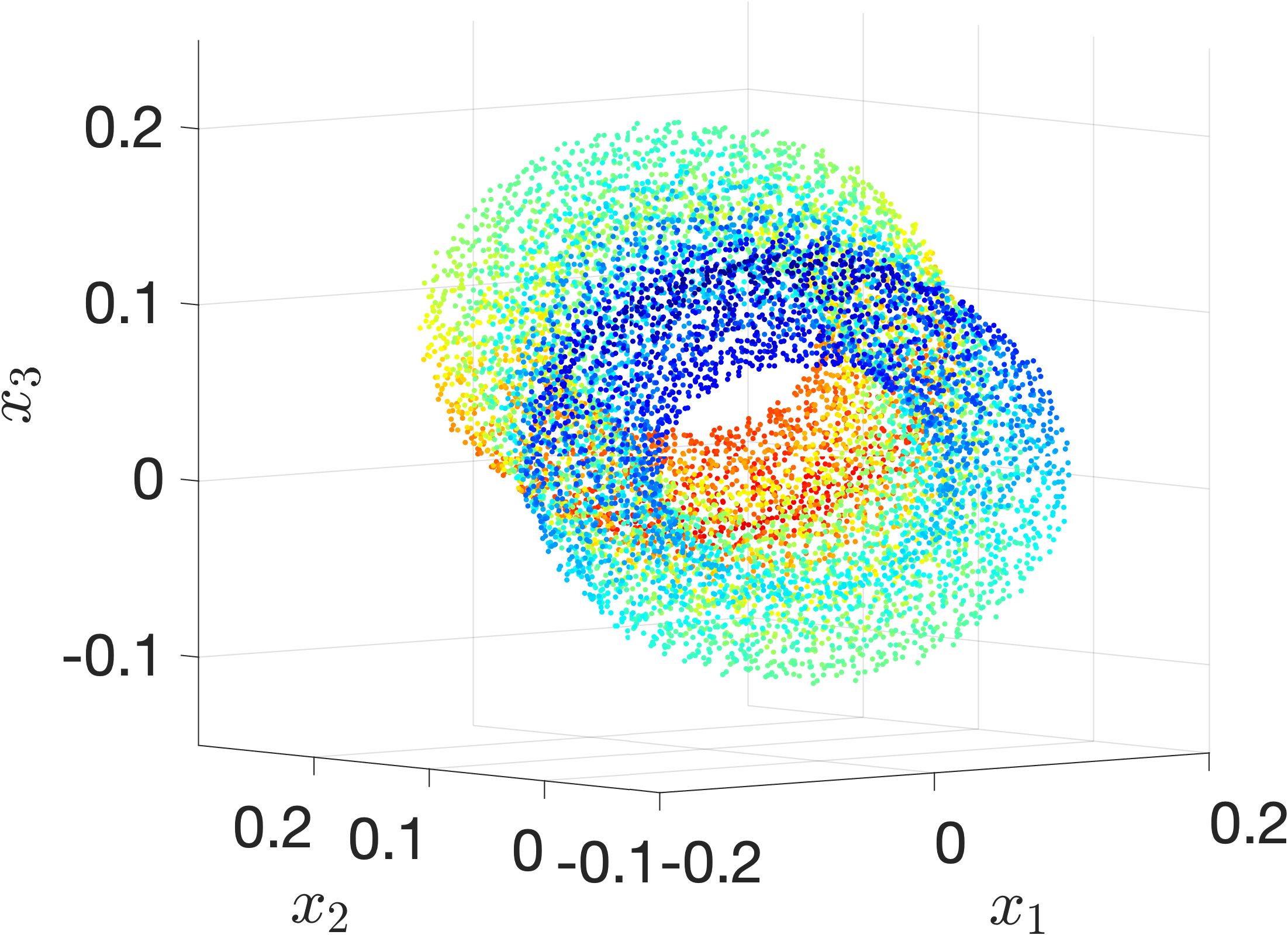
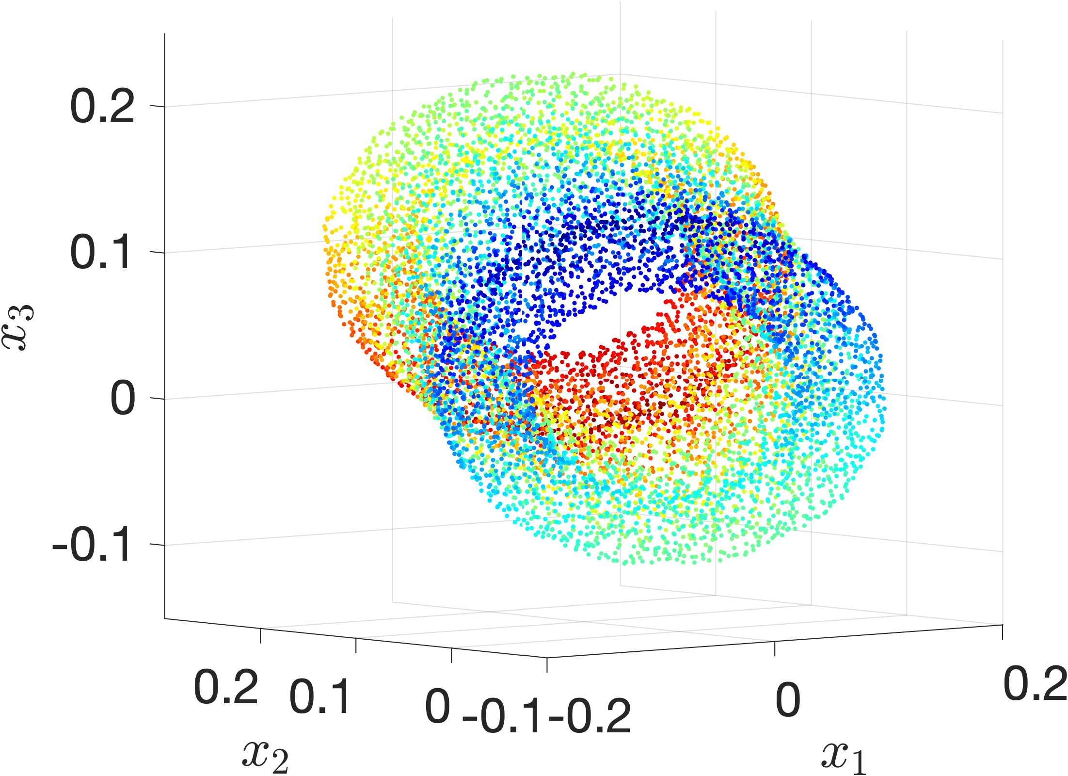
To conclude this section we show some pictures highlighting the numerical validation of the continuum limit we just presented. In particular we compare the orbits of the continuous case, ODE (6.20), with its discrete counterpart, equation (6.4) after applying the scaling (6.17). The two equations are solved in four degrees of freedom with initial values $(\mathbf{x}_{0},\mathbf{x}_{-1})=(0.1,0.1,0.1,0.1,0.1,0,0,0.1)$ , $\alpha=-2$ , $h=0.5$ and $\boldsymbol{\beta}=(0.05,0.2,0.1,0.25)$ . In figure 2 the numerical orbits are plotted. In particular we note that both orbits look very close to an integrable one. Incidentally, this result exhibits another limit of the “orbit method” to identify integrability, see for instance [68, 31]. Finally, figures 3 and 4 show the values of $B_{+}^{(n)}=\boldsymbol{\beta}\cdot\mathbf{x}_{n}$ and $C_{+}^{(n)}=\mathbf{x}_{n}^{2}$ for the continuous case and the discrete case. These two figures highlight a simple oscillatory behaviour, which in both cases mimic the behaviour of the system with one degree of freedom.

7. Conclusions

In this paper we presented a discrete analogue of the coalgebra approach to generate systems in $N$ degrees of freedom as extensions of integrable systems in one degree of freedom. We gave two general results on the integrability properties of two classes of systems of second order difference equation in standard form. Namely, we proved in Theorem 4.3 that all radially-symmetric systems (4.5) are quasi-integrable, and in Theorem 4.7 that all quasi-radially symmetric systems are PLN maps of rank $N-2$ . Up to our knowledge, this is the first time that quasi-integrable discrete systems are produced. Then we considered the following explicit examples of systems in $N$ degrees of freedom:

(1)

A maximally superintegrable radially-symmetric linear equation (4.14) in $N$ degrees of freedom.
(2)

A superintegrable quasi-radially-symmetric linear equation (4.31) in $N$ degrees of freedom.
(3)

A quasi-integrable deformation of the previous system (4.35).
(4)

Two different $N$ degrees of freedom generalisations of the autonomous discrete Painlevé I equation (5.5).
(5)

A non-integrable $N$ degrees of freedom generalisation of the McMillan map (6.4) with many invariants.
(6)

A quasi-maximally superintegrable radially-symmetric $N$ degrees of freedom generalisation of a special case of the McMillan map (6.7).

In particular, the system (4.35) remarkably shows the entropy gap: as soon as $\varepsilon\neq 0$ the $N$ th invariant is missing and the algebraic entropy becomes positive. Despite this the (real) orbits of the system are very regular. Furthermore, we remark that, while some of the systems we considered were known in the literature, up to our knowledge the vector generalisation of the autonomous discrete Painlevé I equation (5.5a) is new.

As usual in discrete systems theory, the discrete case is more complicated than its continuum counterpart: while in the continuum case an $N$ degrees of freedom system is built on top of the $N$ th coproduct of a function, the Hamiltonian, in the discrete setting we define a Poisson map to admit a coalgebra symmetry when the evolution of the generators of the algebra is closed in the algebra and preserves the Casimir of the algebra itself. The last requirement is fundamental since it allows us to prove the existence of the invariants (3.10), and then use the construction to generate systems with $N$ degrees of freedom with a given number of invariants.

The three conditions of Definition 3.3 can be used to build systems admitting the coalgebra symmetry out of general ones. In particular, we highlight with an example that the Casimir condition can greatly help us. For sake of simplicity consider a variational difference equation of standard form (4.1) for $N=2$ with $\mathbf{x}_{n}=(x_{n},y_{n})^{T}$ and the algebra $\mathfrak{sl}_{2}(\mathbb{R})$ . Computing the evolution of the generators of $\mathfrak{sl}_{2}(\mathbb{R})$ we obtain:


(7.1a)	$\displaystyle J_{+}^{(n+1)}$	$\displaystyle=\left[x_{n-1}-\frac{\partial V}{\partial x_{n}}(x_{n},y_{n})\right]^{2}+\left[y_{n-1}-\frac{\partial V}{\partial y_{n}}(x_{n},y_{n})\right]^{2},$
(7.1b)	$\displaystyle J_{-}^{(n+1)}$	$\displaystyle=J_{+}^{(n)},$
(7.1c)	$\displaystyle J_{3}^{(n+1)}$	$\displaystyle=x_{n}\left[x_{n-1}-\frac{\partial V}{\partial x_{n}}(x_{n},y_{n})\right]^{2}+y_{n}\left[y_{n-1}-\frac{\partial V}{\partial y_{n}}(x_{n},y_{n})\right]^{2}.$

We have that the commutation relations of the $\mathfrak{sl}_{2}(\mathbb{R})$ are preserved for all $V$ , while it is not trivial to understand if the right hand side of the expressions in (7.1) are $\mathfrak{sl}_{2}(\mathbb{R})$ . However, it is pretty simple to check if the Casimir (4.10) is preserved. Computing the difference between $C^{(n+1)}$ and $C^{(n)}$ we obtain the simple expression:

(7.2)

\left(x_{n}\frac{\partial V}{\partial y_{n}}-y_{n}\frac{\partial V}{\partial x_{n}}\right)\left[x_{n}y_{n-1}-x_{n-1}y_{n}-\frac{1}{2}\left(x_{n}\frac{\partial V}{\partial y_{n}}-y_{n}\frac{\partial V}{\partial x_{n}}\right)\right]=0.

Since the second factor cannot be zero because $V=V(x_{n},y_{n})$ , the first factor gives us a linear PDE for $V$ . Solving it we obtain $V=V\bigl(\sqrt{x_{n}^{2}+y_{n}^{2}}\bigr)$ . With such value of $V$ we have that the right hand side of the system (7.1) lies in $\mathfrak{sl}_{2}(\mathbb{R})$ . This reasoning can be extended to $N>2$ , and we obtain that the only variational difference equation of standard form (4.1) admitting the $\mathfrak{sl}_{2}(\mathbb{R})$ coalgebra are exactly the radial difference equations (4.5). Note that in this reasoning the variational structure is not restrictive because we are interested in studying integrability.

We remark that in all the examples we presented the associated dynamical system on the generators of the algebra (3.11) is a fundamental tool in studying the integrability of the original difference equation. In this sense the system (3.11) plays a role even more fundamental than the $N$ degrees of freedom Hamiltonian which gives only one additional invariant. This is particularly evident in the case of equation (5.5a) where, due to the presence of the two-photon $h_{6}$ coalgebra, one should have constructed the second invariant with other methods, see [6]. In particular, our examples seem to suggest that the integrability properties of an underlying Poisson map are completely governed by those of the associated dynamical system on the generators of the algebra (3.11). To be more precise, we make this statement rigorous in the following conjecture:

Conjecture.

A Poisson map $T\colon n\mapsto n+1$ admitting a coalgebra symmetry $(\mathfrak{A},\Delta)$ , is Liouville integrable if and only if the evolution of the generators (3.11) is Poisson–Liouville integrable.

This conjecture can be used as a guiding criterion to find more integrable cases, starting from instance from a given coalgebra structure. As we mentioned in the introduction, integrable discrete systems in one degree of freedom are almost completely understood in terms of QRT mappings [50, 51]. QRT mappings have been classified in nine canonical forms in [52]. The additive form (1.2) is the first of these nine canonical forms. We plan to address to the problem of finding the $N$ degrees of freedom version of these maps admitting some notable coalgebra symmetry, like the $\mathfrak{sl}_{2}(\mathbb{R})$ algebra or the $h_{6}$ algebra.

We also note that the production of many examples of discrete integrable systems in $N$ degrees of freedom could help to understand the geometric mechanism behind integrability for systems with many degrees of freedom. Indeed, while for one degree of freedom discrete integrable systems almost all properties can be explained in terms of involution on elliptic curves and fibrations [56, 23, 65], it is known that integrable systems in more degrees of freedom are not always related to elliptic fibrations, see [31, 35, 30].

Finally, we also plan to address to the problem of finding non-autonomous versions of the coalgebraic integrable systems, e.g. with the singularity confinement method [26], and prove rigorously their growth properties with the approach from [69].

Acknowledgements

We thank Prof. Yu. B. Suris for bringing to our attention his interesting papers related to this work.

GG has been supported by Fondo Sociale Europeo del Friuli Venezia Giulia, Programma operativo regionale 2014–2020 FP195673001 (A/Prof. T. Grava and A/Prof. D. Guzzetti).

DL was supported by Australian Research Council Discovery Project DP190101529 (A/Prof. Y.-Z. Zhang).

BKT was supported by the European Unions Horizon 2020 research and innovation programme under the Marie Sklodowska-Curie grant agreement (No. 691070)

Appendix A Algorithm to find integrals of discrete systems

In this appendix we recall briefly a method for finding invariants of birational maps presented first in [24] and recently reprised in [18], where such a result was interpreted in terms of discrete Darboux polynomials.

In the case when a $M$ -dimensional difference equation (2.1) is rational we can transform its map form into a projective map by homogenising the variables. To use all the advantages of projective and algebraic geometry we usually consider the projective space to be defined on the complex field, that is we consider the complex projective space of dimension $M$ , $\mathbb{CP}^{M}$ , with coordinates $[X_{1}:\dots:X_{M+1}]$ . In such a case, we denote the map by $\varphi\colon\mathbb{CP}^{M}\to\mathbb{CP}^{M}$ . In the case when the map possess an inverse $\psi\colon\mathbb{CP}^{M}\to\mathbb{CP}^{M}$ which is a rational map too then the map is said to be birational [57]. Due to birationality the following relations hold:

(A.1)

\psi\circ\varphi=\kappa\Id,\quad\varphi\circ\psi=\lambda\Id,\quad\kappa,\lambda\in\mathbb{C}_{h}\left[x_{1},\cdots,x_{n+1}\right].

The polynomials $\kappa$ and $\lambda$ admit a possibly trivial factorisation of the form:

(A.2)

\kappa=\prod_{i=1}^{K_{\kappa}}\kappa_{i}^{d_{\kappa,i}},\quad\lambda=\prod_{i=1}^{K_{\lambda}}{\lambda}_{i}^{d_{\lambda,i}}.

The map $\varphi$ is ill-defined on the singular locus $V_{\varphi}=\left\{\kappa=0\right\}$ , while the map $\varphi$ is ill-defined on the singular locus $V_{\psi}=\left\{\lambda=0\right\}$ . The singular loci form an algebraic variety of codimension one and measure zero.

In this picture an invariant is a homogeneous function $I=I(X_{1},\dots,X_{M+1})$ such that the pullback

(A.3)

\varphi^{*}(I)(X_{1},\dots,X_{M+1}):=I(\varphi(X_{1},\dots,X_{M+1})),

satisfies $\varphi^{*}(I)=I$ . Now, if the invariant is a ratio of homogeneous polynomials, that is $I\in\mathbb{C}_{h}(X_{1},\dots,X_{M+1})$ , we can write $I=P/Q$ , with $P,Q\in\mathbb{C}_{h}[X_{1},\dots,X_{M+1}]$ . Equation (A.3) implies:

(A.4)

\varphi^{*}(P)=aP\quad\text{and}\quad\varphi^{*}(Q)=aQ

for some polynomial factor $a\in\mathbb{C}_{h}[X_{1},\dots,X_{M+1}]$ . That is the polynomials $P,Q$ are covariant.

To find covariant polynomials we use the fact that the polynomial $a$ must be composed by the factors of the polynomial $\kappa$ , see [24, Lemma 4.1]. So, we can search for invariants imposing the form of $P$ , then searching for the appropriate cofactors, building them from the factorisation (A.2). We get an invariant when we obtain more than one solution for the same $a$ . By taking ratios of the solutions we obtain the invariants.

The disadvantage of this algorithm is that it is not bounded as we don’t know a priori the degree of $P$ . However, in practice this approach is quite useful for the explicit computation of the invariants, since the conditions in (A.4) are linear, even though their number can become huge as $\deg(P)$ and $M$ grow.

Appendix B Algebraic entropy

An integrability criterion unique to birational systems with discrete degrees of freedom is low growth condition [67, 24, 13]. To be specific, we state the following criterion of integrability:

Definition B.1 (Algebraic entropy [13]).

Consider an $M$ -dimensional difference equation (2.1). If the associated projective map $\varphi\colon\mathbb{CP}^{M}\to\mathbb{CP}^{M}$ is birational, then we say that equation (2.1) is integrable in the sense of the algebraic entropy if the following limit

(B.1)

S_{\varphi}=\lim_{k\to\infty}\frac{1}{k}\log\deg\varphi^{k},

called the algebraic entropy is zero for every initial condition.

Algebraic entropy is an invariant of birational maps, meaning that its value is unchanged up to birational equivalence. Practically algebraic entropy is a measure of the complexity of a map, analogous to the one introduced by Arnol’d [1] for diffeomorphisms. In this sense growth is given by computing the number of intersections of the successive images of a straight line with a generic hyperplane in complex projective space [67].

In principle, the definition of algebraic entropy in equation (B.1) requires us to compute all the iterates of a birational map $\varphi$ and take the limit as $k\to\infty$ . However, in the majority of applications, the asymptotic behaviour of the sequence of degrees can be inferred by using generating functions [36]:

(B.2)

g\left(z\right)=\sum_{n=0}^{\infty}d_{k}z^{k},\quad d_{k}=\deg\varphi^{k}.

A generating function is a predictive tool which can be used to test the successive members of a finite sequence. It follows that the algebraic entropy is given by the logarithm of the smallest pole of the generating function, see [27, 25]. A birational map (or its avatar difference equation) will then be integrable if all the poles of the generating function lie on the unit circle.

References

[1] V.. Arnol’d “Dynamics of complexity of intersections” In Bol. Soc. Bras. Mat. 21, 1990, pp. 1–10
[2] Á. Ballesteros and F.. Herranz “Universal integrals for superintegrable systems on N-dimensional spaces of constant curvature” In J. Phys. A: Math. Theor. 40, 2007, pp. F51–F59
[3] Á. Ballesteros, F. Musso and O. Ragnisco “Comodule algebras and integrable systems” In J. Phys. A: Math. Gen. 35, 2002, pp. 8197–8211
[4] A. Ballesteros and A. Blasco “N-dimensional superintegrable systems from symplectic realizations of Lie coalgebras” In J. Phys. A: Math. Theor. 41, 2008, pp. 304028 (18pp)
[5] A. Ballesteros et al. “(Super)integrability from coalgebra symmetry: formalism and applications” In J. Phys.: Conf. Ser. 175, 2009, pp. 012004 (26pp)
[6] A. Ballesteros and F.. Herranz “Two-Photon algebra and integrable Hamiltonian systems” In J. Nonlinear Math. Phys. 8.sup1, 2001, pp. 18–22
[7] A. Ballesteros and O. Ragnisco “A systematic construction of completely integrable Hamiltonians from coalgebras” In J. Phys. A: Math. Gen. 31, 1998, pp. 3791–3813
[8] Á. Ballesteros, A. Enciso, F.. Herranz and O. Ragnisco “A maximally superintegrable system on an n-dimensional space of nonconstant curvature” In Physica D 237, 2008, pp. 505–509
[9] Á. Ballesteros, A. Enciso, F.. Herranz and O. Ragnisco “Superintegrability on N-dimensional curved spaces: Central potentials, centrifugal terms and monopoles” In Ann. Phys. 324, 2009, pp. 1219–1233
[10] Á. Ballesteros et al. “Quantum mechanics on spaces of nonconstant curvature: The oscillator problem and superintegrability” In Ann. Phys. 326, 2011, pp. 2053–2073
[11] Á. Ballesteros and F.. Herranz “Maximal superintegrability of the generalized Kepler–Coulomb system on N-dimensional curved spaces” In J. Phys. A: Math. Theor. 42, 2009, pp. 245203
[12] Á. Ballestreros, M. Corsetti and O. Ragnisco “N-dimensional classical integrable systems from Hopf Algebras” In Czechoslovak J. Phys. 46, 1996, pp. 1153–1163
[13] M. Bellon and C-M. Viallet “Algebraic entropy” In Comm. Math. Phys. 204, 1999, pp. 425–437
[14] M. Bruschi, O. Ragnisco, P.. Santini and G-Z. Tu “Integrable symplectic maps” In Physica D 49.3, 1991, pp. 273–294
[15] G.. Byrnes, F.. Haggar and G… Quispel “Sufficient conditions for dynamical systems to have pre-symplectic or pre-implectic structures” In Physica A 272, 1999, pp. 99–129
[16] H.. Capel and R. Sahadevan “A new family of four-dimensional symplectic and integrable mappings” In Physica A 289, 2001, pp. 80–106
[17] A.. Carstea and T. Takenawa “A classification of two-dimensional integrable mappings and rational elliptic surfaces” In J. Phys. A 45, 2012, pp. 155206 (15pp)
[18] E. Celledoni et al. “Using discrete Darboux polynomials to detect and determine preserved measures and integrals of rational maps” In J. Phys. A: Math. Theor. 52, 2019, pp. 31LT01 (11pp)
[19] V. Chari and A. Pressley “A guide to quantum groups” Cambridge: Cambridge university press, 1995
[20] C. Cresswell and N. Joshi “The discrete first, second and thirty-fourth Painlevé hierarchies” In J. Phys. A: Math. Gen. 32, 1999, pp. 655–669
[21] H. De, P. Iliev, W. vande and L. Vinet “The Racah algebra: An overview and recent results” In Contemp. Math., 2021, pp. 3–20
[22] V.. Drinfel’d “Proc. Int. Congress Math., Berkeley 1986”, 1987 AMS
[23] J.J. Duistermaat “Discrete Integrable Systems: QRT Maps and Elliptic Surfaces”, Springer Monographs in Mathematics Springer New York, 2011
[24] G. Falqui and C-M. Viallet “Singularity, complexity, and quasi-integrability of rational mappings” In Comm. Math. Phys. 154, 1993, pp. 111–125
[25] B. Grammaticos, R.. Halburd, A. Ramani and C-M. Viallet “How to detect the integrability of discrete systems” Newton Institute Preprint NI09060-DIS In J. Phys A: Math. Theor. 42, 2009, pp. 454002 (41 pp)
[26] B. Grammaticos, A. Ramani and V. Papageorgiou “Do integrable mappings have the Painlevé property?” In Phys. Rev. Lett. 67, 1991, pp. 1825
[27] G. Gubbiotti “Integrability of difference equations through Algebraic Entropy and Generalized Symmetries” In Symmetries and Integrability of Difference Equations: Lecture Notes of the Abecederian School of SIDE 12, Montreal 2016, CRM Series in Mathematical Physics Berlin: Springer International Publishing, 2017, pp. 75–152
[28] G. Gubbiotti “On the inverse problem of the discrete calculus of variations” In J. Phys. A: Math. Theor. 52, 2019, pp. 305203 (29pp)
[29] G. Gubbiotti “Lagrangians and integrability for additive fourth-order difference equations” In Eur. Phys. J. Plus 135, 2020, pp. 853 (30pp)
[30] G. Gubbiotti, N. Joshi, D.. Tran and C-M. Viallet “Bi-rational maps in four dimensions with two invariants” In J. Phys. A: Math. Theor 53, 2020, pp. 115201 (24pp)
[31] G. Gubbiotti, N. Joshi, D.. Tran and C-M. Viallet “Complexity and Integrability in 4D Bi-rational Maps with Two Invariants” In Asymptotic, Algebraic and Geometric Aspects of Integrable Systems Cham: Springer International Publishing, 2020, pp. 17–36
[32] J. Hietarinta “Definitions and Predictions of Integrability for Difference Equations” In Symmetries and Integrability of Difference Equations, London Mathematical Society Lecture Notes series Cambridge: Cambridge University Press, 2011, pp. 83–114
[33] J. Hietarinta, N. Joshi and F. Nijhoff “Discrete Systems and Integrability”, Cambridge Texts in Applied Mathematics Cambridge University Press, 2016
[34] E.. Ince “Ordinary Differential Equations”, Dover Books on Mathematics New York: Dover Publications, 1957
[35] N. Joshi and C-M. Viallet “Rational Maps with Invariant Surfaces” In J. Integrable Sys. 3, 2018, pp. xyy017 (14pp)
[36] S.. Lando “Lectures on Generating Functions” American Mathematical Society, 2003
[37] D. Latini “Universal chain structure of quadratic algebras for superintegrable systems with coalgebra symmetry” In J. Phys. A: Math. Theor. 52, 2019, pp. 125202
[38] D. Latini, I. Marquette and Y-Z. Zhang “Embedding of the Racah algebra R(n) and superintegrability” In Ann. Phys. 426, 2021, pp. 168397
[39] D. Latini, I. Marquette and Y-Z. Zhang “Racah algebra R(n) from coalgebraic structures and chains of R(3) substructures” In J. Phys. A: Math. Theor., 2021
[40] D. Latini and D. Riglioni “From ordinary to discrete quantum mechanics: The Charlier oscillator and its coalgebra symmetry” In Phys. Lett. A 380, 2016, pp. 3445–3453
[41] J. Liouville “Note sur l’intégration des équations différentielles de la Dynamique, présentée au Bureau des Longitudes le 29 juin 1853.” In J. Math. Pures Appl. 20, 1855, pp. 137–138
[42] J.. Logan “First integrals in the discrete variational calculus” In Aeq. Math. 9, 1973, pp. 210–220
[43] S. Maeda “Completely integrable symplectic mapping” In Proc. Jap. Ac. A, Math. Sci. 63, 1987, pp. 198–200
[44] R.. McLachlan “Integrable four-dimensional symplectic maps of standard type” In Phys. Lett. A 177, 1993, pp. 211–214
[45] E.. McMillan “A problem in the stability of periodic systems” In A tribute to E.U. Condon, Topics in Modern Physics Boulder: Colorado Assoc. Univ. Press., 1971, pp. 219–244
[46] W.. Miller, S. Post and P. Winternitz “Classical and quantum superintegrability with applications” In J. Phys. A: Math. Theor. 46.42, 2013, pp. 423001
[47] F. Musso “Loop coproducts, Gaudin models and Poisson coalgebras” In J. Phys. A: Math. Theor. 43, 2010, pp. 434026 (17pp)
[48] Fabio Musso “Integrable systems and loop coproducts” In J. Phys. A: Math. Theor. 43, 2010, pp. 455207 (13pp)
[49] S. Post and D. Riglioni “Quantum integrals from coalgebra structure” In J. Phys. A: Math. Theor. 48 IOP Publishing, 2015, pp. 075205
[50] G… Quispel, J… Roberts and C.. Thompson “Integrable mappings and soliton equations” In Phys. Lett. A 126, 1988, pp. 419
[51] G… Quispel, J… Roberts and C.. Thompson “Integrable mappings and soliton equations II” In Physica D 34.1, 1989, pp. 183–192
[52] A. Ramani, A.. Carstea, B. Grammaticos and Y. Ohta “On the autonomous limit of discrete Painlevé equations” In Physica A 305, 2002, pp. 437–444
[53] D. Riglioni “Classical and quantum higher order superintegrable systems from coalgebra symmetry” In J. Phys. A: Math. Theor. 46, 2013, pp. 265207
[54] D. Riglioni, G. Gingras and P. Winternitz “Superintegrable systems with spin induced by co-algebra symmetry” In J. Phys. A: Math. Theor. 47, 2014, pp. 122002
[55] J… Roberts and D. Jogia “Birational maps that send biquadratic curves to biquadratic curves” In J. Phys. A: Math. Theor. 48, 2015, pp. 08FT02
[56] H. Sakai “Rational surfaces associated with affine root systems and geometry of the Painlevé Equations” In Comm. Math. Phys. 220.1, 2001, pp. 165–229
[57] I.. Shafarevich “Basic Algebraic Geometry 1” 213, Grundlehren der mathematischen Wissenschaften Berlin, Heidelberg, New York: Springer-Verlag, 1994
[58] Yu.. Suris “On integrable standard-like mappings” In Funct. Anal. Appl 23, 1989, pp. 74–76
[59] Yu.. Suris “A discrete-time Garnier system” In Phys. Lett. A 189, 1994, pp. 281–289
[60] Yu.. Suris “A family of integrable symplectic standard-like maps related to symmetric spaces” In Phys. Lett. A 192, 1994, pp. 9–16
[61] Yu.. Suris “The problem of integrable discretization: Hamiltonian approach” Basel: Birkhäuser, 2003
[62] T. Tjin “Introduction to quantized Lie groups and algebras” In Int. J. Mod. Phys. A 7, 1992, pp. 6175–6213
[63] D.. Tran “Complete integrability of maps obtained as reductions of integrable lattice equations”, 2011
[64] D.. Tran, P.. van Kamp and G… Quispel “Poisson brackets of mappings obtained as $(q,-p)$ reductions of lattice equations” In Reg. Chaot. Dyn. 21.6 Springer, 2016, pp. 682–696
[65] T. Tsuda “Integrable mappings via rational elliptic surfaces” In J. Phys. A: Math. Gen. 37, 2004, pp. 2721
[66] A.. Veselov “Integrable maps” In Russ. Math. Surveys 46, 1991, pp. 1–51
[67] A.. Veselov “Growth and integrability in the dynamics of mappings” In Comm. Math. Phys. 145, 1992, pp. 181–193
[68] C-M. Viallet “Algebraic dynamics and algebraic entropy” In Int. J. Methods M. 5, 2008, pp. 1373–1391
[69] C-M. Viallet “On the algebraic structure of rational discrete dynamical systems” In J. Phys. A: Math. Theor. 48.16, 2015, pp. 16FT01
[70] C-M. Viallet, B. Grammaticos and A. Ramani “On the integrability of correspondences associated to integral curves” In Phys. Lett. A 322, 2004, pp. 186–93
[71] E.. Whittaker and G.. Watson “A Course of Modern Analysis” Cambridge University Press, 1927
[72] W.-M. Zhang, D.. Feng and R. Gilmore “Coherent states: Theory and some applications” In Rev. Mod. Phys. 62.4, 1990, pp. 867–927

Coalgebra symmetry for discrete systems

Abstract.

2020 Mathematics Subject Classification

1. Introduction

2. Discrete systems and integrability

2.1. Invariants and integrability

Definition 2.1.

Definition 2.2.

Remark 2.1.

Definition 2.3 ([66, 14, 43]).

Remark 2.2.

Definition 2.4 ([66, 14, 43]).

Definition 2.5.

Remark 2.3.

2.2. Variational discrete systems and their integrability

Lemma 2.1 ([14, 33]).

3. Coalgebra symmetry for discrete systems

3.1. Definition of coalgebra and coproduct

Definition 3.1 ([19, 22]).

Definition 3.2.

Remark 3.1.

3.2. Coalgebra symmetry and Liouville integrability

Lemma 3.1 ([7]).

Proof.

Definition 3.3.

Theorem 3.2.

Proof.

3.3. Coalgebra symmetry and superintegrability

Theorem 3.3.

Remark 3.2.

3.4. Final remarks on the coalgebra symmetry

4. General classes of additive differential systems and coalgebra

4.1. Radially symmetric systems and the 𝔰​𝔩2​(ℝ)\mathfrak{sl}_{2}(\mathbb{R}) algebra

Lemma 4.1.

Proposition 4.2.

Remark 4.1.

Proof.

Theorem 4.3.

Example 1.

Remark 4.2.

Remark 4.3.

4.2. Quasi-radially symmetric systems and the h6h_{6} algebra

Lemma 4.4.

Lemma 4.5.

Proposition 4.6.

Remark 4.4.

Proof.

Theorem 4.7.

Example 2.

Remark 4.5.

Example 3.

Remark 4.6.

5. Vector extensions of the autonomous discrete Painlevé I

5.1. Superintegrability of the system (5.5a)

Remark 5.1.

5.2. Superintegrability of the system (5.5b)

Remark 5.2.

5.3. Continuum limits

6. Vector extension of the McMillan map

Remark 6.1.

Remark 6.2.

6.1. Invariants of the system (6.4)

6.2. Quasi-maximal superintegrability of the 𝜷=𝟎\boldsymbol{\beta}=\mathbf{0} case (6.7)

6.3. Continuum limits

7. Conclusions

Conjecture.

Acknowledgements

Appendix A Algorithm to find integrals of discrete systems

Appendix B Algebraic entropy

Definition B.1 (Algebraic entropy [13]).

References

4.1. Radially symmetric systems and the $\mathfrak{sl}_{2}(\mathbb{R})$ algebra

4.2. Quasi-radially symmetric systems and the $h_{6}$ algebra

6.2. Quasi-maximal superintegrability of the $\boldsymbol{\beta}=\mathbf{0}$ case (6.7)