Homography augumented momentum constrastive learning for SAR image retrieval
Abstract
Deep learning-based image retrieval has been emphasized in computer vision. Representation embedding extracted by deep neural networks (DNNs) not only aims at containing semantic information of the image, but also can manage large-scale image retrieval tasks. In this work, we propose a deep learning-based image retrieval approach using homography transformation augmented contrastive learning to perform large-scale synthetic aperture radar (SAR) image search tasks. Moreover, we propose a training method for the DNNs induced by contrastive learning that does not require any labelling procedure. This may enable tractability of large-scale datasets with relative ease. Finally, we verify the performance of the proposed method by conducting experiments on the polarimetric SAR image datasets.
1 Introduction
Deep learning has been applied for synthetic aperture radar (SAR) image analysis tasks such as object detection Chen and Wang 2014, despeckling Tang et al. 2019; Chierchia et al. 2017; Cozzolino et al. 2020, optical data fusion Schmitt et al. 2018, and terrain surface classification Parikh et al. 2020. SAR images can capture the geographic characteristics without depending on the weather conditions. One of the applications is the SAR image retrieval task Noh et al. 2017; Teichmann et al. 2019; DeTone et al. 2018, which aims to retrieve images from a large database that are similar to a query image. This application is further utilized for complementing navigation systems when global positioning system (GPS) is not available Park et al. 2021. For the SAR image retrieval tasks, it is necessary to extract a compressed feature vector from a SAR image while maintaining the semantic information. The vector is then compared with the vectors of SAR images in the database. This technique is sometimes called the global descriptor approach. Convolutional neural networks (CNNs) are frequently used for extracting the global descriptor vectors from the images Gordo et al. 2016; Arandjelovic et al. 2016; Radenović et al. 2016. The global descriptor is a simple vector with a prescribed dimension, thus during testing, distance between vectors can be easily and scalably measured. However, this technique’s overall performance may suffer from complications such as clutter, illumination, and occlusion that all hinder the CNNs from generating adequate global descriptor vectors. To overcome these obstacles, the CNN-based local feature approaches are also suggested Yi et al. 2016; Noh et al. 2017; Teichmann et al. 2019; Cao et al. 2020; DeTone et al. 2018. These methods generate so called keypoints and their local descriptors. The keypoint represents the location of interest and the local descriptor is a vector characterizing an associated keypoint. The CNN-based local feature approaches generally aim to replace the traditional local feature approaches, such as SIFT Lowe 1999; Lowe 2004 or its variants Dellinger et al. 2014. Even though this enhances the performance of retrieving images, comparing image pairs is not scalable, thus it cannot be efficiently applied over the large-scale database. Thus, recent efforts usually focus on developing a CNN-based apporoach combining both global descriptor and local feature approaches; first retrieving images roughly using global descriptor and reranking by utilizing the local feature approach Noh et al. 2017; Park et al. 2021.
In this work, we focus only on the CNN based global descriptor method, which could be a main principle component of the deep learning-based SAR image retrieval system. We propose contrastive learning Hadsell et al. 2006 for generating the global descriptor. Contrastive learning uses multiple neural networks and compares the global descriptors relative to a loss function. To prevent the networks from generating trivial descriptors, homography transformation is applied to augmenting the SAR images. We also demonstrate that the homography transformation can generalize SAR image deformation, thus the homography transformed SAR images are used as an input data for training the networks. Contrastive learning enables the network to learn the features in a self-supervised way, which potentially leads to dealing with a large-scale dataset without involving any arduous labelling process usually done by human labor. To verify the performance of the proposed method, we show experiment results on multiple SAR datasets containing various geographic characteristics.
This paper is organized as follows. Related works of our approach are given in Section 2. In Section 3, a method for generating global descriptor is proposed, which includes contrastive learning and homography transformation. The performance results of the proposed approach on the public SAR dataset are reported in Section 4. Finally, Section 5 presents the conclusions.
2 Related Works
Contrastive learning
Contrastive learning Hadsell et al. 2006 is a self-supervised learning method which has been actively researched recently. It primarily utilizes a comparison between the feature representation pairs of the instances in a representative space to form a loss function. Contrastive learning stems from the idea that the feature vectors of the image and its augmented image are to be located closely while the two feature vectors of two distinguishable images should be located far off. Generally, contrastive learning enables the machine learning system not to rely on labels, but instead, it leads to learning with the pseudo labels generated automatically while comparing the feature vectors during training. In regards to comparing between vectors, it collects vectors from previous iterations and saves them in a memory storage. Contrastive learning can be also utilized for pretraining in a self-supervised manner in order to enhance the performance before applying it for downstream tasks Chen et al. 2021. The primitive attempt, called a memory bank scheme, stores the whole vectors obtained at the previous iterations and uses a subset of them at the current iteration Wu et al. 2018; Park et al. 2021. Since the encoder is gradually updated via backpropagation and a stochastic gradient descent algorithm, the output vectors stored in the memory bank are on occasion incompatible with those produced at the current iteration, which, in turn, leads to slow learning. Further, it involves memory issues due to the notoriously high number of the training data instances. To circumvent this, Momentum Contrast (MoCo) He et al. 2020 uses the Siamese encoder, that is, there are two distinguishable encoders with the same architectures from which the one, primary encoder, is updated with the gradient; whereas the other, momentum encoder, is updated using a momentum rule. Also, it stores the restricted numbers of the key vectors outputted by the momentum encoder into a queue matrix. These are then used when comparing with a query vector outputted by the primary encoder.
There also exist techniques to improve performance of the MoCo mechanism including adding a 2-layer MLP head, blur augmentation, and cosine learning rate schedule Chen et al. 2020a. Recent improvements of MoCo, namely MoCo v3 Chen et al. 2021, suggested an online method generating keys in the same batch to reduce the memory uses while maintaining fast learning. It also uses a form of the infoNCE Oord et al. 2018 as a loss function allowing for representative differentiations between images of a given sufficient batch size (e.g., 4096). Additionally, to further improve the performance of MoCo, they adopted a vision transformation (ViT) Dosovitskiy et al. 2020 as the backbone architecture instead of CNN. There are various approaches in contrastive learning that differ depending on the usages of the queue matrix and the forms of the loss function. They include SimCLR Chen et al. 2020b, SEER Goyal et al. 2021, SwAV Caron et al. 2020, SimSiam Chen and He 2020, and BYOL Grill et al. 2020.
Deep learning-based image retrieval
Deep neural networks (DNNs) have been widely used for representative learning. Traditional components of image retrieval systems, such as SIFT Lowe 1999; Lowe 2004, RANSAC Fischler and Bolles 1981, have been partially replaced by DNN based approaches.
Noh et al. Noh et al. 2017 introduced a method for generating local features using the CNN based model, which can substantially replace the traditional local descriptors such as SIFT. The central point of the receptive field corresponding to the local descriptor represents the keypoint, and the local descriptor is trained with the attention score layer. They also proposed a landmark dataset on which the proposed model is finetuned with the location based image classification labels, which can be regarded as a weakly supervised approach. The performance of this method is further enhanced by applying the regional aggregated selective match kernels Teichmann et al. 2019 and generating both the global descriptor and local features simultaneously Cao et al. 2020. SuperPoint DeTone et al. 2018 outputs both the keypoints and local descriptors simultaneously via a unified CNN-based backbone architecture. Its training process involves pretraining on a synthetic labeled dataset and self-supervised learning with the help of homography transformation.
Park et al. Park et al. 2021 proposed deep cosine similarity neural network to generate a normalized feature vector of a SAR image with the primary purpose of comparing SAR image pairs scalably. The proposed idea of normalizing the vector during training is also equipped in the training process of the encoders used in the present work so as to maintain its norm consistently.
Once similar images from a database are retrieved using the global descriptors, the local features are used for reranking the retrieved images. This process is usually time consuming since matching pairs through RANSAC Fischler and Bolles 1981 or Direct Linear Transformation (DLT) Andrew 2001 is not scalable. Thus, replacing these matching techniques with scalable DNN-based methods is in an active research area where many approaches such as SuperGlue Sarlin et al. 2020 and LoFTR Sun et al. 2021 have been proposed. They also utilize a state-of-the-art architecture, Transformer Vaswani et al. 2017, as their backbone networks, which can significantly enhance performances of the DNN based methods for image retrieval tasks.
3 Methodology
We generate a vector, the (global) feature vector , to compress and represent a SAR image for the purpose of SAR image retrieval. Namely, the vector contains semantic information of the SAR image. In this section, we focus on training a deep neural network based encoder to produce a feature vector that is used in the SAR image retrieval task.
3.1 Contrastive Learning
Contrastive learning has been emphasized recently in the literature as a means for generating feature embedding in a self-supervised way. Generally, it uses the Siamese encoder (twin encoders) that consists of two distinguished CNN based encoders with the same architectures and the same sets of parameters to be learned separately. When two inputs of two different encoders are similar, contrastive learning aims at producing output vectors that are likewise similar; whereas when two inputs are not similar to each other, it should produce outputs that are distinguishable. Contrastive learning allows the encoder to be trained in a self-supervised way; the input data does not need to use labels during training, thus one can aggregate more data for training the model without involving any arduous labor commonly required for labelling instances.
In this work, we use MoCo-like learning He et al. 2020 where the first encoder is updated via a stochastic gradient descent algorithm, whereas the second encoder is updated by a momemtum rule. Fig. 1 depicts the contrastive learning framework that we use for SAR image retrieval. As shown in the figure, two CNN based encoders, the “primary encoder” and the “momentum encoder” , are deployed, where and are the parameter sets corresponding to the former and latter, respectively.

The primary encoder uses a SAR image as an input to produce an output . Similarly, the momentum encoder , which has the same architecture as the primary encoder, uses a transformed SAR image that is drawn from homography transformation based distribution to output a feature vector . The primary encoder is updated using a stochastic gradient descent method where the gradients associated with the parameters are computed through backpropagation. The loss function used for training the primary encoder is described in subsection 3.3. The parameters in the momentum encoder are updated with the momentum rule , where is a momentum parameter used to slowly and stably update parameters . Also, in the momentum encoder, the queue matrix consists of columns of feature vectors calculated during the previous iterations:
| (1) |
where is a prescribed parameter representing the number of feature vectors.
Matrix is continuously enqueued using the most recently generated vectors at the current iteration while the oldest vectors are dequeued to maintain the size of the matrix. It is also emphasized that the momentum encoder uses the transformed SAR image as an input and in this work we consider homography transformation for transforming the SAR images.
3.2 Homography transformation
The transformed input used by the momentum encoder should maintain the same semantic information as the original image, and simultaneously generalize the images in order to prevent trivial training cases. To this end, in the present endeavor we utilize homography transformation. It is known that homography transformation can explain the translational and rotational transformations between an image pair in a same planar space. Thus, it is suitable for tasks such as the one of present interests where SAR images are taken from aircrafts or satellites that are positioned at various altitudes and angles to a specific surface area on a given planar space. Given a pixel location in an original image, homography transformation is a linear transformation represented by a non-singular matrix as
| (2) |
where represents the element of the homography transformation matrix , and is the transformed location. Note that the homography transformation matrix is invariant with scaling, thus containing 8 degrees of freedom. To augment the image data via homography transformation, a 4-point based homography transformation is frequently utilized DeTone et al. 2016; Nguyen et al. 2018. We employ a similar approach furnished in DeTone et al. 2016 to generate the homographic transformed SAR image , which will serve as an input to the momentum encoder.

As shown in Fig. 2, observe that the four corners of the pixel points for (represented as red dots) are drawn at random within the small blue squares. Then, using the four corner points we construct a 4-point parameterization that consists of the , displacements, for . Note that the 4-point parameterization is a matrix containing 8 dofs as the homography transformation matrix , and that can easily be converted to by the DLT algorithm Andrew 2001 or the function getPerspectiveTransform in OpenCV. As shown in the right side of Fig. 2, after applying the homography transformation to an image, the transformed image is cropped so that it is of the same size as the original image. In what follows, with a slight abuse in notation we denote the image distribution of the homography transformation and cropping applied to the image as . The training procedure is presented next.
3.3 Training
The transformed image based on is first sampled and serves as input of the momentum encoder as
| (3) | |||
| (4) |
while the original SAR image is passed as input to the primary encoder. After -normalizing feature vectors and , a logit vector is constructed as follows:
| (5) |
where parameter is called a temperature parameter Hinton et al. 2015; Pereyra et al. 2017. For each SAR image in the training dataset, the loss function takes the form of the infoNCE Oord et al. 2018, i.e.,
| (6) |
where represents the th element of the logit vector . Finally, for the training dataset , the overall loss function for training the primary encoder is given by
| (7) |
The procedure for training the primary encoder and its corresponding momentum encoder is presented in Algorithm 1. As shown in line 9 in Algorithm 1, backpropagation is conducted to calculate the gradients of the loss function w.r.t. the parameters . Stochastic gradient descent or its variants Kingma and Ba 2014; Park et al. 2020 can be applied as to update the parameters , where represents the gradients or their variants used for updating the parameters.
4 Experiments
4.1 SAR image data
As an experimental testbed for SAR image retrieval, we utilize the Uninhabited Aerial Vehicle Synthetic Aperture Radar (UAVSAR) images UAV 2021 from NASA. From the UAVSAR database, we use L-band and the ground projected complex cross (GRD) products of the polarimetric SAR (PolSAR). A central reason for using GRD products is that it provides information on pixel-wise geographic coordinates mapping that, in turn, leads to precise evaluation of performance of image retrieval. Specifically, HHHH, HVHV, VVVV products are processed to grayscale images through ASF MapReady 3.2 software, and grayscale images of HHHH, HVHV, VVVV products correspond to red, green, blue channels of the resulting PolSAR images, respectively.
| Name | Acquisition Date | Size (WH) | Region | Characteristic |
| Haywrd1 | 10/09/2018 | 1977926236 | Hayward fault, CA | Building, Mountain |
| Haywrd2 | 05/30/2019 | 1975826206 | ||
| ykdelB1 | 08/28/2018 | 230073906 | Yukon-Kuskokwim delta, AK | River delta, Tundra |
| ykdelB2 | 09/17/2019 | 231073904 | ||
| atchaf | 04/01/2021 | 64367973 | Atchafalaya river delta, LA | River delta, Vegetation |
| harvrd | 08/17/2009 | 59819319 | Harvard forest, MA | Forest |
| SanAnd | 02/21/2019 | 430506604 | LA basin, CA | Building, Mountain |
| SRIVER | 06/17/2017 | 1663121099 | Subarctic tundra area, AK | Tundra |

Table 1 lists details of the SAR image maps used in our experiments that contain various topological characteristics including building, maintain, river, and vegetation. As shown in the table, the SAR image maps are too big to serve as input for the encoders. Thus, we extract patches of size with a stride of pixels from the images. Since GRD formatting is arranged to locate the north to the upper side of an image map with respect to the geographic coordinates, it may contains a lot of “blank” area (shown as black region as in Fig. 3). Further, as the blank area does not contain any meaningful information, we eliminate this by using the local descriptor method, SAR-SIFT Dellinger et al. 2014. For each extracted patch, we generated the keypoints by SAR-SIFT and patches with at least 200 keypoints were added to the datasets in our experiments. It was deemed that a patch with less than 200 keypoints contains a significant amount of black area. The resulting patches were then resized to pixels. Homography transformation was applied “on the fly” during training. On the resized SAR patches, i.e., pixels, four points were drawn at random, from the four corner squares of pixels centered at the corner points (shown as the dashed blue lines in Fig. 2) to estimate .

For each experiment, three types of datasets consisting of the SAR patches were prepared: the query dataset, training dataset, and key dataset as shown in Fig. 4. Each of the patches in the datasets has at least 1000 SAR-SIFT based keypoints. The primary encoder and momentum encoder are trained on the training dataset whereas the SAR patches in the query dataset are used for testing. During testing, we extract the patches with similar feature vectors to the query patch from the key dataset which is also regarded as a database. We restrict the number of patches in the query dataset to 100 which are selected at random.
| Exp. Num. | Exp. Name | Query set | Key set | Training set | ||
|---|---|---|---|---|---|---|
| Exp.1 | Haywrd-Easy | Haywrd2 (100) | Haywrd1, ykdelB1 (20388) | Haywrd1 (12979) | ||
| Exp.2 | Haywrd-Hard | Haywrd2 (100) | Haywrd1, ykdelB1 (20388) |
| ||
| Exp.3 | ykdelB-Easy | ykdelB2 (100) | Haywrd1, ykdelB1 (20388) | ykdelB1 (7409) | ||
| Exp.4 | ykdelB-Hard | ykdelB2 (100) | Haywrd1, ykdelB1 (20388) |
|
To verify the performance of the proposed approach, we set up four experiments that simulate multiple operational circumstances, as shown in Table 2. The query sets are Haywrd2 or ykdelB2. Those are relatively recently acquired than the key datasets, Haywrd1 and ykdelB1 (Please see Table 1). For experiment 1 and 3 (Exp.1 and Exp.3), which is harder experiments, we have used Haywrd1 and ykdelB1 as the training datasets, respectively. For these experiments, the training datasets were the same as the key datasets, hence the encoders have already observed similar SAR image patches to the query images during training. It is therefore anticipated that the encoders would be able to generate more accurate feature vectors for these two experiments compared to the experiment cases 2 and 4 (Exp.2 and Exp.4).
For these easier experiments (Exp.2 and Exp.4), the encoders had not observed the same patches during training; instead, it was trained on the training dataset consisting of patches from atchaf, harvrd, SanAnd and SRIVER SAR maps. Also for all experiments, the Haywrd1 and ykdelB1 are used as the key dataset.
4.2 Architecture and Settings
All experiments used ResNet50 or ResNet101 He et al. 2016 as a backbone CNN architecture. The CNNs were pretrained on the ImageNet dataset Deng et al. 2009. From the output map of the conv4 layer of ResNet, we adopted generalized mean (GeM) pooling Radenović et al. 2018 that weighs the importance of the outputs to generate the feature vector. Denote that the output map of the conv4 layer as , where and are indices of height and width locations of the image, respectively. We further integrated GeM pooling followed by a fully connected layer, parameterized by weights and bias , similar to the approach in Gordo et al. 2017; Cao et al. 2020. The feature vector that summarizes the discriminative outputs of the image is produced as an output of the GeM pooling layer as
| (8) |
where , represent the height and width of the output map, and is the parameter of the GeM pooling. In our experiments parameter is set to 3. The feature vector is then normalized.
For training we employed the Adam optimizer Kingma and Ba 2014 with a learning rate of that gets decreased by after epochs. The maximum number of epochs was set to 100 and the batch size for training is 32. The temperature parameter was set to without performing any hyperparameter tunings. For contrastive learning parameters, the queue size and the momentum parameter . To prevent feature vector from having an excessively high norm, prior to normalization we added the regularization term derived in Park et al. 2021 into the loss function. Specifically, this term is simply denoted as . The coefficient of the regularization was set to .
Note that when testing the image retrieval performance, since focus is put on measuring the performance of the feature vector, we do not consider any approximate techniques for measuring distance such as query expansion Chum et al. 2007; Radenović et al. 2018 or asymmetric quantizer distance Cao et al. 2016.
4.3 Experiments Results
| Method | mAP | mP@1 | mP@10 | mP@50 |
|---|---|---|---|---|
| Exp.1 Haywrd-Easy | ||||
| ResNet50-512 | 0.5254 | 1.0000 | 0.9870 | 0.8044 |
| ResNet50-1024 | 0.4908 | 1.0000 | 0.9810 | 0.7702 |
| ResNet101-512 | 0.5366 | 0.9700 | 0.9650 | 0.8018 |
| ResNet101-1024 | 0.5314 | 0.9800 | 0.9630 | 0.7952 |
| Exp.2 Haywrd-Hard | ||||
| ResNet50-512 | 0.4092 | 1.0000 | 0.9810 | 0.6874 |
| ResNet50-1024 | 0.4287 | 1.0000 | 0.9730 | 0.7188 |
| ResNet101-512 | 0.4223 | 1.0000 | 0.9690 | 0.7050 |
| ResNet101-1024 | 0.4159 | 1.0000 | 0.9650 | 0.6976 |
| Exp.3 ykdelB-Easy | ||||
| ResNet50-512 | 0.4708 | 0.9700 | 0.9230 | 0.6128 |
| ResNet50-1024 | 0.4439 | 0.9100 | 0.8640 | 0.5760 |
| ResNet101-512 | 0.4296 | 0.9400 | 0.8690 | 0.5644 |
| ResNet101-1024 | 0.4290 | 0.9500 | 0.8630 | 0.5574 |
| Exp.4 ykdelB-Hard | ||||
| ResNet50-512 | 0.4181 | 0.9400 | 0.8440 | 0.5750 |
| ResNet50-1024 | 0.3916 | 0.9600 | 0.8340 | 0.5442 |
| ResNet101-512 | 0.3681 | 0.9700 | 0.8680 | 0.5138 |
| ResNet101-1024 | 0.3682 | 1.0000 | 0.8970 | 0.5280 |
To measure performance, we define precision and recall as follows. Recall is the total number of the retrieved SAR patches from the database (key dataset), and precision is defined as the ratio between the number of accurately retrieved SAR patches and the total number of the retrieved SAR patches. When there are the duplicate regions calculated in terms of the geographic coordinates between the query image and the retrieved image, we consider the retrieved image as the accurately retrieved image. As a primary performance measure, we have used mean average precision (mAP). The average precision is the mean value of the precision values obtained at various recall values for each query image. In the present setting, the mAP is the mean of the average precision values over 100 query images. Also, the mean precision at (mP@n) is used as a performance measure where represents the recall value. We report three mean precisions; mP@1, mP@10, mP@50. For instance, it is implied that when we retrieve ten SAR patches from the database, mP@10 represents the fraction of the number of the accurate images we can expect to retrieve correctly.
The experiment results are shown in Table 3. The methods vary depending on the dimension of the feature output , which is 512 or 1024, and the two considered architectures ResNet50 or ResNet101.
The “Haywrd” cases (Exp.1 and Exp.2) are from the Hayward fault in California, USA, and predominantly consists of human-made structures. The “ykdelB” cases (Exp.3 and Exp.4) on the other hand, mostly consist of natural formations. By comparing the mAP values, we observed that the proposed method more effectively retrieved similar images for the Haywrd experiment cases compared to the ykdelB cases. For both datasets, it can be seen that mAP values of the “Hard” cases are lower than those of the “Easy” cases.
Although the performances are relatively lower in the hard cases, it can be observed that the proposed method works well regardless of the dimension of the feature vector and the backbone architectures, as even mP@1 results in high values (over 0.9) in all the experiments. This result strongly indicates that our method can perform remarkably well without the use of any sophisticated yet non-scalable methods such as local descriptors Noh et al. 2017 and matching through RANSAC Fischler and Bolles 1981.
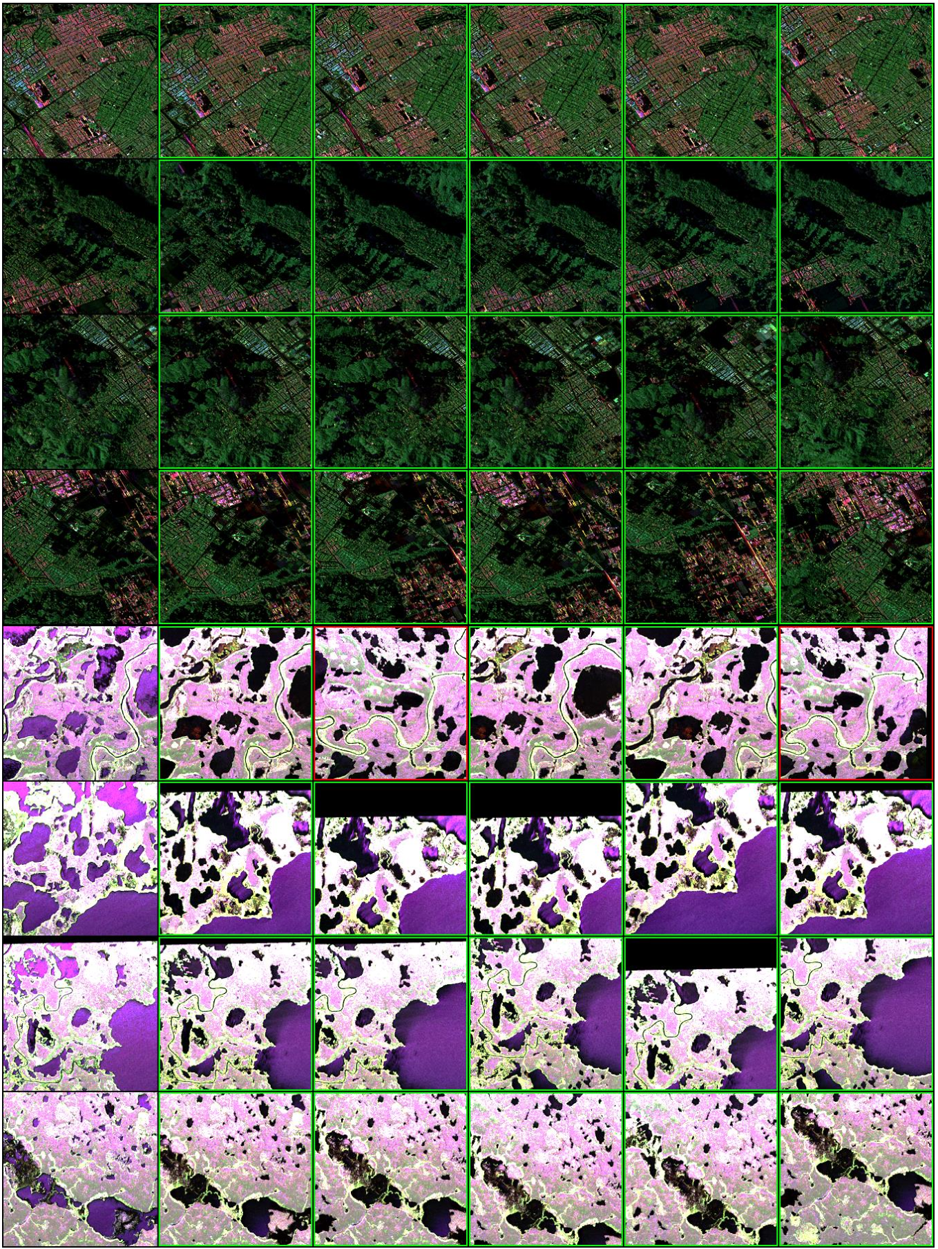
By way of visual results, Fig. 5 shows several retrieved SAR patches using ResNet101-1024 that outputs 1024 dimensional feature vector and its backbone is ResNet101. In most cases, the proposed method retrieves SAR images correctly from the database. In fact, only two retrieved images in the Exp.4 ykdelB-Hard case were incorrect; however, these images are quite similar with a query SAR image.
5 Conclusions
In this paper, we have proposed a contrastive learning method for the SAR image retrieval task. To this end, homography transformation is used for augmenting the SAR image patches and the output vector of a transformed image is compared against that of an original image. This enables the proposed encoders to be trained in a self-supervised manner, thus no labelling process is necessary for establishing the dataset. The proposed method is therefore especially applicable for tasks where the labelling process is time consuming. Experiments were conducted and the results demonstrate that even in the cases where the encoders have not seen similar SAR images to a given query image, it nevertheless successfully retrieves similar SAR images from the database. This work can be utilized for applications such as image searching based positioning or navigation, which is one our future extensions.
References
- Chen and Wang (2014) Sizhe Chen and Haipeng Wang. Sar target recognition based on deep learning. In 2014 International Conference on Data Science and Advanced Analytics (DSAA), pages 541–547. IEEE, 2014.
- Tang et al. (2019) Xiao Tang, Lei Zhang, and Xiaoli Ding. Sar image despeckling with a multilayer perceptron neural network. International Journal of Digital Earth, 12(3):354–374, 2019.
- Chierchia et al. (2017) Giovanni Chierchia, Davide Cozzolino, Giovanni Poggi, and Luisa Verdoliva. Sar image despeckling through convolutional neural networks. In 2017 IEEE International Geoscience and Remote Sensing Symposium (IGARSS), pages 5438–5441. IEEE, 2017.
- Cozzolino et al. (2020) Davide Cozzolino, Luisa Verdoliva, Giuseppe Scarpa, and Giovanni Poggi. Nonlocal cnn sar image despeckling. Remote Sensing, 12(6):1006, 2020.
- Schmitt et al. (2018) Michael Schmitt, Lloyd Haydn Hughes, and Xiao Xiang Zhu. The sen1-2 dataset for deep learning in sar-optical data fusion. arXiv preprint arXiv:1807.01569, 2018.
- Parikh et al. (2020) Hemani Parikh, Samir Patel, and Vibha Patel. Classification of sar and polsar images using deep learning: a review. International Journal of Image and Data Fusion, 11(1):1–32, 2020.
- Noh et al. (2017) Hyeonwoo Noh, Andre Araujo, Jack Sim, Tobias Weyand, and Bohyung Han. Large-scale image retrieval with attentive deep local features. In Proceedings of the IEEE international conference on computer vision, pages 3456–3465, 2017.
- Teichmann et al. (2019) Marvin Teichmann, Andre Araujo, Menglong Zhu, and Jack Sim. Detect-to-retrieve: Efficient regional aggregation for image search. In Proceedings of the IEEE/CVF Conference on Computer Vision and Pattern Recognition, pages 5109–5118, 2019.
- DeTone et al. (2018) Daniel DeTone, Tomasz Malisiewicz, and Andrew Rabinovich. Superpoint: Self-supervised interest point detection and description. In Proceedings of the IEEE conference on computer vision and pattern recognition workshops, pages 224–236, 2018.
- Park et al. (2021) Seonho Park, Maciej Rysz, Kaitlin L Fair, and Panos M Pardalos. Synthetic-aperture radar image based positioning in gps-denied environments using deep cosine similarity neural networks. Inverse Problems & Imaging, 2021.
- Gordo et al. (2016) Albert Gordo, Jon Almazán, Jerome Revaud, and Diane Larlus. Deep image retrieval: Learning global representations for image search. In European conference on computer vision, pages 241–257. Springer, 2016.
- Arandjelovic et al. (2016) Relja Arandjelovic, Petr Gronat, Akihiko Torii, Tomas Pajdla, and Josef Sivic. Netvlad: Cnn architecture for weakly supervised place recognition. In Proceedings of the IEEE conference on computer vision and pattern recognition, pages 5297–5307, 2016.
- Radenović et al. (2016) Filip Radenović, Giorgos Tolias, and Ondřej Chum. Cnn image retrieval learns from bow: Unsupervised fine-tuning with hard examples. In European conference on computer vision, pages 3–20. Springer, 2016.
- Yi et al. (2016) Kwang Moo Yi, Eduard Trulls, Vincent Lepetit, and Pascal Fua. Lift: Learned invariant feature transform. In European conference on computer vision, pages 467–483. Springer, 2016.
- Cao et al. (2020) Bingyi Cao, André Araujo, and Jack Sim. Unifying deep local and global features for image search. In European Conference on Computer Vision, pages 726–743. Springer, 2020.
- Lowe (1999) David G Lowe. Object recognition from local scale-invariant features. In Proceedings of the seventh IEEE international conference on computer vision, volume 2, pages 1150–1157. Ieee, 1999.
- Lowe (2004) David G Lowe. Distinctive image features from scale-invariant keypoints. International journal of computer vision, 60(2):91–110, 2004.
- Dellinger et al. (2014) Flora Dellinger, Julie Delon, Yann Gousseau, Julien Michel, and Florence Tupin. Sar-sift: a sift-like algorithm for sar images. IEEE Transactions on Geoscience and Remote Sensing, 53(1):453–466, 2014.
- Hadsell et al. (2006) Raia Hadsell, Sumit Chopra, and Yann LeCun. Dimensionality reduction by learning an invariant mapping. In 2006 IEEE Computer Society Conference on Computer Vision and Pattern Recognition (CVPR’06), volume 2, pages 1735–1742. IEEE, 2006.
- Chen et al. (2021) Xinlei Chen, Saining Xie, and Kaiming He. An empirical study of training self-supervised visual transformers. arXiv preprint arXiv:2104.02057, 2021.
- Wu et al. (2018) Zhirong Wu, Yuanjun Xiong, Stella X Yu, and Dahua Lin. Unsupervised feature learning via non-parametric instance discrimination. In Proceedings of the IEEE Conference on Computer Vision and Pattern Recognition, pages 3733–3742, 2018.
- He et al. (2020) Kaiming He, Haoqi Fan, Yuxin Wu, Saining Xie, and Ross Girshick. Momentum contrast for unsupervised visual representation learning. In Proceedings of the IEEE/CVF Conference on Computer Vision and Pattern Recognition, pages 9729–9738, 2020.
- Chen et al. (2020a) Xinlei Chen, Haoqi Fan, Ross Girshick, and Kaiming He. Improved baselines with momentum contrastive learning. arXiv preprint arXiv:2003.04297, 2020a.
- Oord et al. (2018) Aaron van den Oord, Yazhe Li, and Oriol Vinyals. Representation learning with contrastive predictive coding. arXiv preprint arXiv:1807.03748, 2018.
- Dosovitskiy et al. (2020) Alexey Dosovitskiy, Lucas Beyer, Alexander Kolesnikov, Dirk Weissenborn, Xiaohua Zhai, Thomas Unterthiner, Mostafa Dehghani, Matthias Minderer, Georg Heigold, Sylvain Gelly, et al. An image is worth 16x16 words: Transformers for image recognition at scale. arXiv preprint arXiv:2010.11929, 2020.
- Chen et al. (2020b) Ting Chen, Simon Kornblith, Mohammad Norouzi, and Geoffrey Hinton. A simple framework for contrastive learning of visual representations. In International conference on machine learning, pages 1597–1607. PMLR, 2020b.
- Goyal et al. (2021) Priya Goyal, Mathilde Caron, Benjamin Lefaudeux, Min Xu, Pengchao Wang, Vivek Pai, Mannat Singh, Vitaliy Liptchinsky, Ishan Misra, Armand Joulin, et al. Self-supervised pretraining of visual features in the wild. arXiv preprint arXiv:2103.01988, 2021.
- Caron et al. (2020) Mathilde Caron, Ishan Misra, Julien Mairal, Priya Goyal, Piotr Bojanowski, and Armand Joulin. Unsupervised learning of visual features by contrasting cluster assignments. arXiv preprint arXiv:2006.09882, 2020.
- Chen and He (2020) Xinlei Chen and Kaiming He. Exploring simple siamese representation learning. arXiv preprint arXiv:2011.10566, 2020.
- Grill et al. (2020) Jean-Bastien Grill, Florian Strub, Florent Altché, Corentin Tallec, Pierre H Richemond, Elena Buchatskaya, Carl Doersch, Bernardo Avila Pires, Zhaohan Daniel Guo, Mohammad Gheshlaghi Azar, et al. Bootstrap your own latent: A new approach to self-supervised learning. arXiv preprint arXiv:2006.07733, 2020.
- Fischler and Bolles (1981) Martin A Fischler and Robert C Bolles. Random sample consensus: a paradigm for model fitting with applications to image analysis and automated cartography. Communications of the ACM, 24(6):381–395, 1981.
- Andrew (2001) Alex M Andrew. Multiple view geometry in computer vision. Kybernetes, 2001.
- Sarlin et al. (2020) Paul-Edouard Sarlin, Daniel DeTone, Tomasz Malisiewicz, and Andrew Rabinovich. Superglue: Learning feature matching with graph neural networks. In Proceedings of the IEEE/CVF conference on computer vision and pattern recognition, pages 4938–4947, 2020.
- Sun et al. (2021) Jiaming Sun, Zehong Shen, Yuang Wang, Hujun Bao, and Xiaowei Zhou. Loftr: Detector-free local feature matching with transformers. arXiv preprint arXiv:2104.00680, 2021.
- Vaswani et al. (2017) Ashish Vaswani, Noam Shazeer, Niki Parmar, Jakob Uszkoreit, Llion Jones, Aidan N Gomez, Lukasz Kaiser, and Illia Polosukhin. Attention is all you need. arXiv preprint arXiv:1706.03762, 2017.
- DeTone et al. (2016) Daniel DeTone, Tomasz Malisiewicz, and Andrew Rabinovich. Deep image homography estimation. arXiv preprint arXiv:1606.03798, 2016.
- Nguyen et al. (2018) Ty Nguyen, Steven W Chen, Shreyas S Shivakumar, Camillo Jose Taylor, and Vijay Kumar. Unsupervised deep homography: A fast and robust homography estimation model. IEEE Robotics and Automation Letters, 3(3):2346–2353, 2018.
- Hinton et al. (2015) Geoffrey Hinton, Oriol Vinyals, and Jeff Dean. Distilling the knowledge in a neural network. arXiv preprint arXiv:1503.02531, 2015.
- Pereyra et al. (2017) Gabriel Pereyra, George Tucker, Jan Chorowski, Łukasz Kaiser, and Geoffrey Hinton. Regularizing neural networks by penalizing confident output distributions. arXiv preprint arXiv:1701.06548, 2017.
- Kingma and Ba (2014) Diederik P Kingma and Jimmy Ba. Adam: A method for stochastic optimization. arXiv preprint arXiv:1412.6980, 2014.
- Park et al. (2020) Seonho Park, Seung Hyun Jung, and Panos M Pardalos. Combining stochastic adaptive cubic regularization with negative curvature for nonconvex optimization. Journal of Optimization Theory and Applications, 184(3):953–971, 2020.
- UAV (2021) Dataset: UAVSAR POLSAR, NASA 2021. Retrieved from ASF DAAC, 22 April 2021.
- He et al. (2016) Kaiming He, Xiangyu Zhang, Shaoqing Ren, and Jian Sun. Deep residual learning for image recognition. In Proceedings of the IEEE conference on computer vision and pattern recognition, pages 770–778, 2016.
- Deng et al. (2009) Jia Deng, Wei Dong, Richard Socher, Li-Jia Li, Kai Li, and Li Fei-Fei. Imagenet: A large-scale hierarchical image database. In 2009 IEEE conference on computer vision and pattern recognition, pages 248–255. Ieee, 2009.
- Radenović et al. (2018) Filip Radenović, Giorgos Tolias, and Ondřej Chum. Fine-tuning cnn image retrieval with no human annotation. IEEE transactions on pattern analysis and machine intelligence, 41(7):1655–1668, 2018.
- Gordo et al. (2017) Albert Gordo, Jon Almazan, Jerome Revaud, and Diane Larlus. End-to-end learning of deep visual representations for image retrieval. International Journal of Computer Vision, 124(2):237–254, 2017.
- Chum et al. (2007) Ondrej Chum, James Philbin, Josef Sivic, Michael Isard, and Andrew Zisserman. Total recall: Automatic query expansion with a generative feature model for object retrieval. In 2007 IEEE 11th International Conference on Computer Vision, pages 1–8. IEEE, 2007.
- Cao et al. (2016) Yue Cao, Mingsheng Long, Jianmin Wang, Han Zhu, and Qingfu Wen. Deep quantization network for efficient image retrieval. In Proceedings of the AAAI Conference on Artificial Intelligence, volume 30, 2016.