Ionizing radiation from AGNs at with the Subaru Hyper Suprime-Cam Survey and the CFHT Large Area U-band Deep Survey (CLAUDS)2021Ionizing radiation from AGNs at with the Subaru Hyper Suprime-Cam Survey and the CFHT Large Area U-band Deep Survey (CLAUDS)–A
Abstract
We use deep and wide imaging data from the CFHT Large Area U-band Deep Survey (CLAUDS) and the Hyper Suprime-Cam Subaru Strategic Program (HSC-SSP) to constrain the ionizing radiation (Lyman Continuum; LyC) escape fraction from AGNs at . For 94 AGNs with spectroscopic redshifts at , we use their -band / -band flux ratios to estimate LyC transmission of individual AGNs. The distribution of their LyC transmission shows values lower than the range of LyC transmission values for IGM of the same redshift range, which suggests that LyC escape fraction of AGNs at is considerably lower than unity in most cases. We do not find any trend in LyC transmission values depending on their UV luminosities. Based on the photometry of stacked images we find the average flux ratio of LyC and non-ionizing UV photons escaping from the objects for AGNs at , which corresponds to LyC escape fraction if we assume a fiducial intrinsic SED of AGN. Based on the estimated LyC escape fraction and the UV luminosity function of AGNs, we argue that UV-selected AGNs’ contribution to the LyC emissivity at the epoch is minor, although the size of their contribution largely depends on the shape of the UV luminosity function.
Keywords:
galaxies: active – galaxies: evolution – galaxies:high-redshift – intergalactic medium – cosmology: observations.1 Introduction
Active Galactic Nuclei (AGNs) and massive stars in star-forming galaxies are the two primary sources of hydrogen-ionizing radiation (Lyman Continuum; LyC hereafter) in the Universe. Understanding the relative contributions from these two populations to the ionizing photon budget over cosmic time is deeply connected to our understanding of AGN and star-formation activity in galaxies at different epochs.
In light of measurements of the faint-end galaxy UV luminosity function (UVLF) at high redshift, it has been suggested that faint galaxies are the population primarily responsible for reionizing the Universe (Inoue et al. 2006; Robertson et al. 2013; Dressler et al. 2015; Finkelstein et al. 2015; Ishigaki et al. 2015, e.g.,). However, maintaining reionization is not easy even with the large number of faint galaxies that are observed: even if the UVLF is integrated beyond the current observing limits, relatively high ionizing photon escape fractions, %, are needed to keep intergalactic space ionized. In contrast, direct constraints on for star-forming galaxies at infer relatively low average values of 10% (Steidel et al. 2018; Iwata et al. 2019, e.g.,). This tension suggests that in galaxies may be luminosity-dependent or may increase at higher redshift (Inoue et al. 2006). Alternatively, an additional source of ionizing photons may be required.
Several studies based on the observations of the quasar UVLF have reported that the AGN contribution to the ionizing photon budget is minor (Willott et al. 2010; Onoue et al. 2017; Akiyama et al. 2018; Kulkarni et al. 2019). However, Giallongo et al. 2015 argued that the steep faint-end slope of the AGN UVLF they found for X-ray selected AGNs at would imply that AGN could provide enough photons to keep the Universe ionized. This view is supported by Boutsia et al. 2018 who argued that, based on spectroscopy of faint AGNs in the COSMOS field, the number density of faint AGNs could be higher than found by earlier studies, and that, consequently, AGNs could make a substantial contribution to the ionizing photon budget (see also Giallongo et al. 2019, Grazian et al. 2020 and Boutsia et al. 2021 for further reports on high AGN space density at ). Clearly, an accurate determination of the AGN UVLF is critically important to give us a definitive evaluation of the AGN contribution to the ionizing photon budget. But another critical parameter to be understood here is the ionizing radiation escape fraction for AGNs.
Previous studies often assumed on the supposition that ionizing photons emerging from the AGN can efficiently escape into the intergalactic space. However, studies of for AGNs at based on direct measurement of their LyC have shown that this assumption could be wrong (Cristiani et al. 2016; Micheva et al. 2017a; Grazian et al. 2018; Romano et al. 2019; Smith et al. 2020), although the number of AGN used in these studies is still small, except Cristiani et al. 2016 and Romano et al. 2019 who examined of large numbers of bright quasars from SDSS at . Given the potential importance of AGN in reionizing the Universe, it is therefore important to better constrain the AGN and its dependence on AGN luminosity.
The goal of the present paper is to constrain based on a large sample of AGNs with a broad range of UV luminosity. Here, we turn to the Deep layer of the HSC Subaru Strategic Program (Aihara et al. 2018; Aihara et al. 2019, HSC-SSP;) which we combine with very deep -band images from the Canada-France-Hawaii Telescope (CFHT) Large Area U-band Deep Survey (Sawicki et al. 2019, CLAUDS, ). These two surveys cover 19 deg2 with very deep imaging to an unprecedented combination of area and depth; they span enough volume with sufficient sensitivity to contain a significant population of high- AGNs with a wide range of luminosities (more than 2 orders of magnitude in flux at rest-frame 1400Å). Together with a large spectroscopic sample of 94 AGNs at that we assembled in these fields from the literature, the deep CLAUDS -band images allow us to measure the ionizing flux escaping from each spectroscopically-confirmed AGN, while the HSC-SSP photometry at longer wavelengths provides their non-ionizing UV luminosity.
Throughout this paper we use AB magnitudes and assume the (, , ) = (0.3, 0.7, 70 km s-1 Mpc-1) cosmology.
2 Data
This study uses very deep observed-frame -band11 1 Depending on the field, CLAUDS uses u-band and u∗-band filters (Sawicki et al. 2019). We refer these two bandpass filters collectively as -band. fluxes to determine the amount of ionizing photons escaping from AGN located at redshifts . Photometry at longer wavelengths is used to determine the intrinsic AGN luminosity which is needed to convert the escaping ionizing flux into the ionizing photon escape fraction. Accurate redshifts are essential for the AGN to ensure that the -band contains only ionizing radiation. For these reasons our data consist of a sample of AGNs with spectroscopic redshifts (described in Section 2.1) and photometry from two very deep, overlapping imaging surveys (Section 2.2).
2.1 Sample AGNs
We use the imaging data from CLAUDS and HSC-SSP deep survey which consist of four independent fields (XMM-LSS, Extended-COSMOS, ELAIS-N1, and DEEP2-3) with areas of 4–6 deg2 each and 18.60 deg2 in total and with imaging (Section 2.2). We compiled a list of AGNs in the fields from the literature in the redshift range between =3.3 and 4.0. Our list consists of 94 AGNs and contains only AGNs with redshifts marked as highly reliable based on detections of multiple emission lines. We excluded AGNs which are only listed in the catalogue of PRIMUS (Coil et al. 2011; Cool et al. 2013) even if their redshifts in the catalogue are between 3.3 and 4.0, as reliability of the redshift listed in the catalogue is not high for high redshift objects. In Tables 1, 2, and 4 we give the positions, spectroscopic redshifts, absolute magnitudes at rest-frame 1450 Å, type of AGN (broad-line AGN (‘BLA’) or narrow-line AGN (‘NLA’)) in literature if available, references and their designations in the references. For the AGNs in the SXDS / XMM-LSS field, we only use those at redshift larger than 3.4, as only u∗-band images are available in this field and in the u∗-band image there would be significant (%) contributions from non-ionizing photons for objects at .
| SXDS / XMM-LSS | |||||||||||
|---|---|---|---|---|---|---|---|---|---|---|---|
| ID | R.A.(J2000) | Decl.(J2000) | Redshift | Filter | Type | N/Ea | Ref.b | Designation | |||
| S01 | 3.5120 | u∗ | BLA | N | 01,01 | SXDS0016 | |||||
| S03 | 3.5190 | u∗ | BLA | N | 02,02 | SDSS021613.88040827.2 | |||||
| S07 | 3.4220 | u∗ | NLA | E | 01,01 | SXDS0422 | |||||
| S10 | 3.9806 | u∗ | BLA | N | 03,01 | SXDS0459 | |||||
| S11 | 3.9832 | u∗ | BLA | N | 04,01 | VANDELS_UDS_199159 | |||||
| S13 | 3.5110 | u∗ | – | E | 05,– | IRS_AAOmega:AAO_SMA_047 | |||||
| S14 | 3.8570 | u∗ | BLA | E | 01,01 | SXDS0809 | |||||
| S15 | 3.6990 | u∗ | BLA | N | 01,01 | SXDS0824 | |||||
| S16 | 3.5530 | u∗ | BLA | N | 01,01 | SXDS0835 | |||||
| S19 | 3.7611 | u∗ | BLA | N | 06,06 | VIPERS:123049002 | |||||
| S20 | 3.6400 | u∗ | BLA | N | 06,06 | VIPERS:124045929 | |||||
| S22 | 3.7148 | u∗ | BLA | N | 07,07 | N_19_46 | |||||
| S24 | 3.8466 | u∗ | BLA | N | 07,07 | N_66_19 | |||||
| S25 | 3.5333 | u∗ | BLA | N | 02,02 | SDSS022236.43033840.7 | |||||
| S30 | 3.6719 | u∗ | BLA | N | 07,07 | N_97_11 | |||||
| S31 | 3.8653 | u∗ | BLA | N | 07,07 | N_11_3 | |||||
| S35 | 3.7790 | u∗ | BLA | N | 02,02 | SDSS022413.41052724.8 | |||||
| S37 | 3.4905 | u∗ | BLA | N | 07,07 | N_50_45 | |||||
| S38 | 3.8527 | u∗ | BLA | N | 08,08 | VVDSDEEP:020254576 | |||||
| S40 | 3.4147 | u∗ | BLA | N | 02,02 | SDSS022543.53042834.5 | |||||
| S41 | 3.5900 | u∗ | – | N | 05,– | 2XLSSdJ022545.0043736 | |||||
| S42 | 3.8600 | u∗ | BLA | N | 08,08 | VVDSDEEP:020290592 | |||||
| S44 | 3.5700 | u∗ | – | N | 05,– | 2XLSSdJ022630.8041326 | |||||
| S48 | 3.7400 | u∗ | – | E | 05,– | 2XLSSdJ022741.9043605 | |||||
| S49 | 3.6260 | u∗ | BLA | N | 08,08 | VVDSDEEP:020277536 | |||||
| S50 | 3.7407 | u∗ | BLA | N | 02,02 | SDSS022754.61044535.5 | |||||
| S52 | 3.6581 | u∗ | BLA | N | 07,07 | N_105_36 | |||||
Notes. a: ‘N’ stands for a nuclear-dominated AGN, while ‘E’ stands for an extended AGN (see Section 3.2).
b: References. The first reference is for redshift, and the second one is for AGN type. 01: Akiyama et al. 2015, 02: SDSS quasar catalog DR14 (Pâris et al. 2018), 03: He et al., in prep., 04: VANDELS DR2 (Pentericci et al. 2018), 05: M. Akiyama, private communication, 06: VIPERS PDR2 (Cucciati et al. 2017), 07: Menzel et al. 2016, 08: VVDS (Le Fèvre et al. 2013).
| COSMOS | |||||||||||
|---|---|---|---|---|---|---|---|---|---|---|---|
| ID | R.A.(J2000) | Decl.(J2000) | Redshift | Filter | Type | N/Ea | Ref.b | Designation | |||
| C07 | 3.6095 | u | BLA | N | 09,09 | COSMOS_J095753.49+024736.1 | |||||
| C08 | 3.9860 | u | – | N | 10,– | B18_0664641 | |||||
| C10 | 3.9600 | u | BLA | E | 11,11 | L450105 | |||||
| C11 | 3.3030 | u | NLA | N | 11,11 | lid_1808 | |||||
| C12 | 3.5240 | u | BLA | E | 12,09 | COSMOS_J095901.31+024418.8 | |||||
| C13 | 3.3260 | u | BLA | N | 11,11 | L772453 | |||||
| C14 | 3.7480 | u | BLA | N | 10,10 | B18_1730531 | |||||
| C15 | 3.3600 | u | BLA | N | 13,13 | M12_1511846 | |||||
| C16 | 3.6300 | u | BLA | N | 10,10 | B18_1938843 | |||||
| C17 | 3.6860 | u | NLA | E | 11,11 | lid_2189 | |||||
| C18 | 3.3710 | u | BLA | N | 12,12 | XMMC_149.85099+2.27609 | |||||
| C19 | 3.3450 | u | BLA | N | 12,12 | XMMC_149.86981+2.29391 | |||||
| C20 | 3.6510 | u | BLA | N | 12,12 | XMMC_149.87949+2.22567 | |||||
| C21 | 3.3350 | u | NLA | E | 11,11 | cid_1134 | |||||
| C22 | 3.3600 | u | BLA | N | 14,13 | L747071 | |||||
| C23 | 3.3170 | u | BLA | N | 14,14 | L1040434 | |||||
| C24 | 3.4990 | u | BLA | N | 12,12 | XMMC_150.00412+2.03904 | |||||
| C25 | 3.3430 | u | NLA | E | 11,11 | lid_1244 | |||||
| C26 | 3.3600 | u | BLA | N | 13,13 | PRIMUS_110535 | |||||
| C27 | 3.5460 | u | NLA | E | 15,15 | CCOS1505 | |||||
| C28 | 3.9490 | u | BLA | E | 14,14 | L862385 | |||||
| C29 | 3.4100 | u | BLA | N | 13,13 | M12_0790476 | |||||
| C30 | 3.8650 | u | BLA | N | 14,13 | L768961 | |||||
| C31 | 3.3330 | u | BLA | N | 12,12 | XMMC_150.20888+2.48202 | |||||
| C32 | 3.7150 | u | BLA | N | 12,12 | XMMC_150.20929+2.43844 | |||||
| C33 | 3.3560 | u | BLA | N | 12,09 | XMMC_150.24087+2.65873 | |||||
| C34 | 3.7470 | u | BLA | N | 14,14 | L179154 | |||||
| C35 | 3.7170 | u | BLA | N | 11,13 | M12_1208399 | |||||
| C36 | 3.7580 | u | BLA | N | 14,14 | C1432719 | |||||
| C37 | 3.8460 | u | BLA | E | 14,14 | L405213 | |||||
| C38 | 3.5120 | u | NLA | N | 11,11 | cid_1656 | |||||
| C39 | 3.3280 | u | BLA | N | 12,12 | XMMC_150.29764+2.14830 | |||||
| C40 | 3.4980 | u | NLA | E | 15,15 | CCOS784 | |||||
| C41 | 3.8400 | u | BLA | N | 13,13 | L368476 | |||||
| C42 | 3.3100 | u | NLA | E | 11,11 | cid_3293 | |||||
| C43 | 3.4820 | u | NLA | E | 11,11 | cid_1672 | |||||
| C44 | 3.3280 | u | BLA | E | 14,12 | L554731 | |||||
| C45 | 3.8590 | u | – | E | 16,– | CCOS879 | |||||
| C46 | 3.4870 | u | NLA | E | 11,11 | lid_4112 | |||||
| C47 | 3.5710 | u | NLA | E | 11,11 | cid_2949 | |||||
| C49 | 3.4650 | u | BLA | N | 09,09 | COSMOS_J100145.58+024212.6 | |||||
A list of sample AGNs in the COSMOS field. COSMOS ID R.A.(J2000) Decl.(J2000) Redshift Filter Type N/Ea Ref.b Designation C50 3.4710 u BLA N 11,11 L441487 C51 3.5600 u BLA N 13,13 M12_1628943 C52 3.6500 u BLA N 13,13 M12_1159815 C53 3.7490 u BLA N 12,12 XMMC_150.70394+2.36961 C54 3.5675 u BLA E 11,11 L419634 C55 3.4970 u∗ BLA N 11,12 lid_1710 C56 3.3020 u BLA N 12,09 COSMOS_J100256.92+024321.2 C57 3.6260 u∗ BLA N 10,10 B18_0899256 C59 3.7720 u – N 10,– B18_0247934 C60 3.6800 u BLA N 03,03 VVDSWIDE:100359356 C61 3.5570 u BLA N 03,03 VVDSWIDE:100105943 C62 3.4035 u BLA N 02,02 SDSS100502.75+012426.3
Notes. a: ‘N’ stands for a nuclear-dominated AGN, while ‘E’ stands for an extended AGN (see Section 3.2).
b: References. The first reference is for redshift, and the second one is for AGN type. 02: SDSS quasar catalog DR14 (Pâris et al. 2018), 03: VVDS Le Fèvre et al. 2013, 09: Trump et al. 2009, 10: Boutsia et al. 2018, 11: Marchesi et al. 2016, 12: Brusa et al. 2010, 13: Masters et al. 2012, 14: Hasinger et al. 2018, 15: Civano et al. 2012, 16: Vito et al. 2014.
| ELIAS-N1 | |||||||||||
| ID | R.A.(J2000) | Decl.(J2000) | Redshift | Filter | Type | N/Ea | Ref.b | Designation | |||
| E01 | 3.3370 | u | BLA | N | 02 | SDSS160647.69+543449.6 | |||||
| E03 | 3.5080 | u | BLA | N | 02 | SDSS160934.12+550015.1 | |||||
| E04 | 3.4050 | u | BLA | N | 02 | SDSS160947.88+552542.7 | |||||
| E05 | 3.9290 | u | BLA | N | 02 | SDSS161107.45+534208.1 | |||||
| E07 | 3.5830 | u | BLA | N | 02 | SDSS161143.22+553157.3 | |||||
| DEEP2-3 | |||||||||||
| D03 | 3.5440 | u | BLA | N | 02 | SDSS232352.94003942.7 | |||||
| D04 | 3.5850 | u | BLA | N | 02 | SDSS232433.92005849.3 | |||||
| D07 | 3.6590 | u | BLA | N | 02 | SDSS232522.84002439.1 | |||||
| D08 | 3.7940 | u | BLA | N | 02 | SDSS232557.46005458.3 | |||||
| D09 | 3.6760 | u | BLA | N | 02 | SDSS232717.95+000545.7 | |||||
| D10 | 3.6370 | u | BLA | N | 02 | SDSS232850.03+004059.0 | |||||
| D11 | 3.3980 | u | BLA | N | 02 | SDSS232910.12+001337.9 | |||||
| D12 | 3.4490 | u | BLA | N | 02 | SDSS233049.38000357.2 | |||||
| D13 | 3.3360 | u | BLA | N | 02 | SDSS233052.60003510.6 | |||||
Notes. a: ‘N’ stands for a nuclear-dominated AGN, while ‘E’ stands for an extended AGN (see Section 3.2).
b: 02: SDSS quasar catalog DR14 (Pâris et al. 2018).
Fig. 1 shows the distribution of redshifts and absolute magnitudes at rest-frame 1450Å for our sample of AGNs. We calculate the magnitude of each AGN through a K-correction procedure that uses the synthetic colour calculated from a fiducial quasar spectrum to infer the magnitude at rest-frame 1450Å from the observed i-band magnitude. The fiducial spectrum comes from Lusso et al. 2015 and is based on the HST Wide Field Camera 3 spectra of 53 quasars at with correction of absorption by IGM. The K-correction calculation is expressed as
| (1) |
which we can expand as
| (2) |
where the synthetic colour is the difference between magnitude at rest-frame 1450Å and i-band magnitude for the fiducial AGN spectrum at the observed redshift, and is a luminosity distance to the object. With cosmology fixed, the only uncertainty in Equation 2 is due to the synthetic colour term, which could in principle be eliminated (as, for example, in Sawicki & Thompson 2006) by using the observed magnitude (instead of our ) as observed-frame corresponds closely to rest-frame 1450Å at our redshifts. However, we use i-band instead of r-band because at the r-band filter could contain the Ly emission line and, consequently, the flux -band flux density could strongly deviate from the continuum flux density. Nevertheless, while non-zero, is still small and fairly constant, ranging over 0.15–0.22 mag depending on the object’s redshift. The values we calculated are listed in Tables 1, 2, and 4. The sample AGNs used in this study come from multiple catalogs in the literature and contain both X-ray selected and optically selected AGNs. We have compiled as many AGNs with reliable spectroscopic redshifts as possible, and there is no uniform selection criteria. Nevertheless, as Fig. 1 shows, there is no strong selection bias in terms of UV luminosity, and even in the higher redshift range UV-faint AGNs are included in the sample.
2.2 Photometric data
For photometry in , , , , and -bands, we use the HSC SSP S20A internal data release. We also tested photometry with the S18A data release which was processed using an older version of the pipeline and is identical to the second public data release (Aihara et al. 2019, PDR2;). We confirmed that choice of the data release does not alter our findings on the LyC transmission from the sample AGNs significantly. At shorter wavelengths, we use the u-band and u∗-band observations provided by CLAUDS (Sawicki et al. 2019). The median depth of the data is =27.1 AB (5 in 2″ apertures), and there is a 1.36 deg2 sub-area in the COSMOS field with a median depth of =27.7 AB (5 in 2″ apertures). The median seeing size (FWHM) of the CLAUDS -band data is 092, while for the HSC SSP Deep+UltraDeep data they are 081, 074, 062, 071 for , , , , -bands, respectively (Aihara et al. 2019).
In Fig. 2, throughput of the systems with these bandpass filters are shown in the rest-frame wavelengths for sources at , along with the stacked quasar spectrum by Lusso et al. 2015. At , u-band is free from non-ionizing photons, while for u∗-band there are some contributions by non-ionizing photons for sources at , because the filter transmission slope is shallower than u-band and there is also a small leak around Å. In Section 3.3 we will correct for such effects of non-ionizing photons. For the COSMOS field all the objects except two have both u-band and u∗-band images (the remaining two have only u∗-band image). We use u-band for those objects if both are available. For the objects in the ELIAS-N1 and DEEP2-3 fields only u-band images are available, and in the SXDS/XMM-LSS field only u∗-band images are available.
3 Analysis
3.1 Photometry
The coordinates of the sample AGNs are taken from their positions in the
HSC SSP database,
which is based on the -band images.
For photometry in the HSC bands we use PSF model-based photometry
[grizy]_psfflux_mag
and its error [grizy]_psfflux_magerr in the forced catalog of the
database. For u and u∗-band images, we used photutils
(Bradley
et al. 2019) to obtain 15-diameter aperture
photometry.
Uncertainties were estimated with the help of artificial point sources
inserted into the images. The procedure is described in
Appendix A.
If an object’s flux density is more than three times higher than the
1 error of the image, we regard the object is detected in
u or u∗-band , and use PSF model-based photometry in the HSC SSP
database, which employs the same algorithm used for photometry in HSC
bandpass filters, as its -band magnitude. Otherwise the object is
regarded as undetected in -band, and 15-diameter aperture
photometry value is used to set the 3 upper-limit of its flux
density.
We visually inspected postage stamp images of the all sample AGNs and
found that there is no object which has significant detection in
-band with a spatial offset relative to i-band.
Finally, foreground Galactic dust extinction corrections were applied to all the photometric data. Here we used the dust reddening map by Schlegel et al. 1998, with the calibration by Schlafly & Finkbeiner 2011, obtained from the NASA/IPAC IRSA web service22 2 https://irsa.ipac.caltech.edu/applications/DUST/.
In Fig. 3 colours of the sample AGNs are plotted against their redshifts. The average colours of the sample AGNs are also plotted, in 0.1 redshift steps. When we calculate the average we simply use the lower limit values for those not detected in -band. Therefore these average values should be taken as lower limits. In the figure we also show the expected colours if we use the stacked quasar spectrum by Lusso et al. 2015 as a fiducial intrinsic SED, apply average IGM attenuation at the redshift using a prescription given by Inoue et al. 2014, and assume . The expected colours increase along redshift, due to increased average IGM attenuation. The observed colours of the sample AGNs roughly follow the trend of the expected colours, although there are large dispersions in the observed colours. As described in Section 2.1, the sample AGNs in this study come from multiple sources and no uniform selection criterion was adopted. Prochaska et al. 2009 examined colours of SDSS quasars and found that colours of 3.5 quasars are systematically redder than those at 3.6. They argued that the SDSS colour-selection criteria would introduce such selection bias. From Fig. 3, we do not see evidence for a bias of this type in terms of colours for the sample AGNs in the present study. The measured colours of individual objects are given in Tables 1, 2, and 4.
3.2 Selection of nuclear-dominated AGNs
As described in Section 3.3, we need to assume an intrinsic SED of AGN to estimate the LyC transmission and escape fraction. For that purpose, we use the stacked quasar spectrum by Lusso et al. 2015 as a template of intrinsic AGN SED. If the flux of an AGN is not dominated by its nucleus but its host galaxy significantly contributes to its flux, we should use a different SED to properly estimate the LyC transmission. However, it is difficult to estimate the intrinsic SED when the nuclear photons do not dominate the SED. Thus we focus on sub-sample of AGNs dominated by nuclear emission. In order to do so, we use the difference between magnitudes in -band measured by fitting PSF () and those with photometry using galaxy surface density profile model fitting (Bosch et al. 2018, CModel;), . We use the following criterion to select nuclear-dominated AGNs:
| (3) |
This criterion means that flux density measured with galaxy model fitting needs to be 15% or less larger than the flux density measured with PSF fitting. Although this criterion is arbitrary, it eliminates most of the AGNs which are classified as NLAs in literature among the sample AGNs. As shown in Fig. 4, all but two objects among 12 NLA AGNs have magnitude difference larger than 0.15, and through visual inspection we find that the objects with magnitude difference larger than 0.15 generally show extended morphologies in the HSC images.
Among 94 sample AGNs, 74 objects satisfy this criterion. We refer this subsample as ‘nuclear-dominated’ AGNs and this subsample is used to estimate LyC transmission and escape fraction.
3.3 Estimation of LyC transmission
We use u and u∗-band photometry to estimate LyC emissivity and transmission of the target AGNs. Rest-frame wavelength ranges traced by these photometric data vary depending on redshift of the source. For u-band the rest-frame wavelength ranges traced by the filter with 50% of the peak throughput are 800 – 924 Å and 688 – 795Å for an object at and , respectively, and for u∗-band they are 789 – 936 Å and 694 – 824 Å for an object at and , respectively. For u-band at about 90% of photons have 912Å (for both a template AGN SED and an SED that is flat in ), and at all photons collected with this filter are LyC. On the other hand, for u∗-band , about 23% of photons from a source at are non-ionizing UV photons, and due to a small red leak in the filter transmission around 5030 Å(see Fig. 2), a few per cent of the photons collected with the filter is expected to be non-ionizing photons even for a source at . We need to correct for contributions from such non-ionizing photons to calculate LyC emissivity of the target AGNs.
LyC transmission for an object we want to know is defined as
| (4) |
where and are the observed and intrinsic LyC flux densities, respectively. Note that includes attenuation by both ISM and IGM. On the other hand, the escape fraction of LyC is the ratio of LyC luminosity going out from an object to that generated within the object:
| (5) |
and the relation between and can be expressed as:
| (6) |
where is IGM opacity for the sightline of the object. Because is unknown, we do not derive for individual sources, but calculate only . We will estimate using stacking analysis in Section 3.5.
Similar to , transmission of non-ionizing UV photon is
| (7) |
If -band contains non-ionizing photons, the sum of and equals to the observed flux densities in u or u∗-band , . For and we use a mean QSO spectrum by Lusso et al. 2015 as an intrinsic SED. In Section 4.1 we discuss how our estimates of LyC transmission change if the assumed intrinsic SED is changed.
For AGNs observed with u-band filter at , all photons collected by u-band filter are LyC photons, and we can simply use Eq. 4 to calculate LyC transmission. For AGNs observed with u∗-band filter or those with u-band filter and at , we need to estimate the amount of non-ionizing UV photons in the observation and subtract it to obtain :
| (8) |
In order to estimate , we need to take the fluctuation of caused by the intervening IGM into account. An absorber at a redshift close to the source produces both the LyC absorption and the Ly absorption, and the degree of these absorption is determined by the opacity of the absorber. However, LyC photons travelling toward us can be also absorbed by an absorber at lower redshift due to Ly absorption. This makes a variation in the values of for sightlines toward sources at a redshift with a certain value of Ly absorption, leading to an uncertainty in estimating and . In order to consider the effect of such uncertainty, we use the results of Monte Carlo simulation of IGM transmission (Inoue & Iwata 2008) which generate 10,000 sightlines for redshifts consistent with the Hi cloud distribution defined analytically by Inoue et al. 2014. First we use the mean UV transmission from 10,000 realizations of the sightlines with the redshift of a sample AGN to make an initial estimate of LyC transmission, :
| (9) |
Then we extract 1,000 instances from Monte Carlo realizations with in the range of 33 3 Changing the range of from Monte Carlo realization does not affect the best estimate value of in most cases. By selecting sightlines with and instead of , the changes in resultant best estimate values are less than 10% for 69 and 60 objects out of the 74 sample AGNs, respectively. The largest change in is %.. These simulated sightlines are used to get the distribution of , and then to derive the mean value of , which is used as the best estimate of LyC transmission of the object. The standard deviation of values is added to the error estimate of in addition to the photometric errors.
In Tables 1, 2, and 4 values calculated with this procedure are provided. Among 74 nuclear-dominated sample AGNs, 41 objects are undetected (i.e., have flux densities less than ) in u-band or u∗-band images. For these objects, we estimate the upper limit of in the same manner as detected sources but using upper limit flux density in u-band or u∗-band , and if the estimated , which equals to , exceeds the value of the upper limit flux density (i.e., upper limit of is negative), we cannot put any constraint on for the object. There are 14 such cases.
3.4 Distribution of LyC transmission
In Fig. 5 the distribution of LyC transmission () of the 60 sample AGNs (14 objects with negative upper-limit among 74 objects are removed) is plotted against their redshifts. If u/u∗-band measured flux densities are below the 3 detection limit then the values based on the 3 limits are presented as long as the upper limit values are larger than the expected non-ionizing photon flux densities. Note that includes attenuation by IGM. As the redshift of a target AGN increases, the frequency of high IGM opacity along the sightline becomes higher, as indicated by the solid lines and shaded areas in Fig. 5. The distribution of values for individual AGN also reflects this increase of IGM opacity with redshift. Note that the majority of the data points are under the average IGM transmission (solid lines), which means that the average of the sample AGNs is smaller than unity.
To examine if there is a UV luminosity dependence on LyC transmission, in Fig. 6 values are plotted against AGN’s absolute magnitudes at rest-frame 1450Å. In the left panel of the figure we show the distribution of values of the nuclear-dominated AGNs at . In the right panel of the figure we also show the distribution of AGNs at , a narrower redshift range where average IGM attenuation is relatively smaller than that for higher redshift. There are 38 AGNs in the redshift range. In both panels we also plot the median and mean values in 0.5 magnitude bins, as well as the variation of median values estimated by bootstrap resampling. In calculation of median and mean values and variations, we use values based on 15-diameter aperture photometry even if the values are negative, while we use 3 upper-limits if objects are not detected in -band when plotting of individual AGNs. No clear dependence on UV luminosity is seen in neither panel. In the next subsection we further examine if there is any UV luminosity dependence on LyC radiation from AGNs, through stacking analysis.
In Fig. 6 there appears to be a gap in the distribution of for both sample AGNs at and those at ; a group of AGNs has while others have around 0.1–0.3. In Fig. 7, we show the histograms of of the sample AGNs. For those without detection in -band, we adopt 3 upper-limits of . We also show the histograms of LyC transmission of IGM, which is equivalent to the case when . Those are generated using the results of Monte Carlo realization of IGM distribution calculated for 10,000 sightlines per redshift in 0.1 step between and 4.0, and are combined with weighted average based on the redshift distribution of the sample AGNs. From Fig. 7 we see that the distribution of the sample AGNs is more clustered towards lower values than that of IGM, which is also clearly seen in Fig. 5. Such distribution indicates that LyC escape fraction of the sample AGNs is considerably less than unity in most cases. We also see that there is a second peak of at in the distribution of the sample AGNs. It should be reminded that the bimodality of LyC escape fraction has been suggested in past studies on LyC escape of star-forming galaxies (Micheva et al. 2017b; Nakajima et al. 2020, e.g.,) and luminous quasars at (Cristiani et al. 2016). The distribution found in Fig. 6 and 7 may imply that LyC escape fraction distribution of AGNs studied here also has a bimodal distribution. Unfortunately, statistical significance is marginal due to a small number of the sample AGNs, and there is a non-negligible possibility that such bimodal distribution can be observed even if AGNs have a single value or their intrinsic distributes uniformly among certain values between 0 and 1, due to the variance of IGM attenuation. To confirm the bimodality of we need larger sample of AGNs.
3.5 Average LyC escape fraction from stacking analysis
We use the 38 objects in the redshift range among the nuclear-dominated AGNs, including both with and without -band detections, for stacking analysis. First, subsections of u-band or u∗-band images centred at their -band centroid positions are extracted. We mask objects (except the sample AGNs) detected by running SExtractor version 2.19.5 (Bertin & Arnouts 1996) with 5 connected pixels above 2 as a threshold. The local background value is estimated by getting a median value of the count distribution for a area around the object after iterations of 2 clipping, and the value is subtracted from the image so that the median background value becomes zero. We then normalise the images with their diameter aperture flux density at rest-frame 1450Å. The flux density at rest-frame 1450Å of an object is derived from which is estimated in the way described in Section 2.1. We also correct for IGM attenuation by dividing the images with mean IGM transmission with u / u∗-band at the object’s redshift, using the transmission formulation by Inoue et al. 2014. The mean image is then generated by taking a mean of the array of counts for each pixel. Measurement of the integrated counts with diameter aperture gives the average .
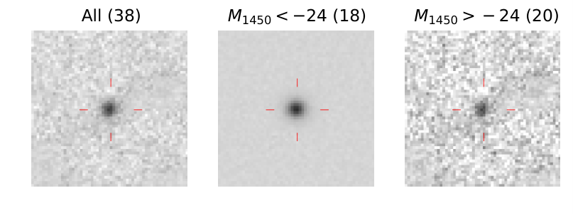
To search for indications of luminosity dependence on the LyC escape fraction, we also generate stacked images of two subsamples based on absolute UV magnitude. For this, we generate stacks with 18 objects and 20 objects with and , respectively. In Fig. 8 we show the stacked image with the full sample of 38 objects, as well as images for two subgroups.
In the stacking procedure we assume the mean IGM attenuation for all objects. This assumption would be valid to estimate the mean flux ratio if the number of stacked objects is sufficiently large. We estimate the effect of fluctuation in IGM transmission by randomly selecting sightlines from Monte Carlo IGM realisations and taking averages of their IGM transmissions. With 10,000 tests the standard deviation of the average IGM transmission is 11% for 38 sightlines and 15–17% for 18 and 20 sightlines. These fluctuations are taken into account when we estimate the error in stacking analysis to derive average . Additionally, we execute bootstrap resampling of the images used for stacking and include the resulting scatter in the error budget of our measurements. It should be also noted that we ignore any possible deviation of average IGM opacity around the sample AGNs from the average value determined from the observations of Lyman absorbers (Inoue et al. 2014). Strong ionizing radiation from AGNs may efficiently ionize neutral hydrogen surrounding them and make their surrounding environment more transparent to the ionizing radiation (Scott et al. 2000, proximity effect; e.g.,). On the other hand, AGNs may reside in the peaks of matter distribution of the universe and Hi column density in the vicinity of the AGNs may be higher than the average. Prochaska et al. 2013 used close pairs of quasars at different redshifts to find an excess of Ly absorption in the transverse direction of quasars, with a correlation length of 12.5 Mpc for optically thick ( cm-2) absorbers. Interestingly, Hennawi & Prochaska 2007 argues that such excess of absorbers is not observed in the the line of sight direction and claims anisotropic ionizing radiation of quasars. Although there are such possible complexities in the Hi gas distribution in the vicinity of AGNs, we consider that it is fair to adopt the mean IGM attenuation to estimate in this study, because FWHMs of the filter transmission are 530Å and 647Å for u-band and u∗-band respectively, which correspond to 550 Mpc in comoving scale for an object at . We measure LyC transmission along such a long line of sight and therefore the effect of AGN environment in the Hi column density would be insignificant.
Table 5 summarises the measured values of average for the 38 AGNs as well as bright and faint subgroups. Median stacked images are also generated, and their values are also shown in the Table. The error sizes of bright and faint subsamples are larger than those of the stacking of all objects, because the errors are dominated by fluctuations in bootstrap tests and IGM transmission rather than background noise, and a standard deviation with smaller number of sample objects is larger. We see no significant difference between for the brighter subgroup and that for the fainter one, which is also suggested by the distribution of LyC transmission distribution of individual objects shown in Fig. 6. Here we do not take non-ionizing photons contained in u / u∗-band into account. Although the flux densities of non-ionizing photons from individual objects are unknown, if we assume the intrinsic SED (Lusso et al. 2015) and use the mean IGM attenuation (Inoue et al. 2014) at the redshifts of the sample AGNs, the expected normalized counts of non-ionizing photons in the stacked image is 0.013. The numbers of shown in Table 5 would be smaller by 0.01 if we were able to subtract non-ionizing photons from the u / u∗-band images.
The measured value can be translated into LyC escape fraction with an assumption of the intrinsic flux ratio between LyC and UV (at rest-frame 1450Å) by
| (10) |
With the fiducial model SED, at the average redshift of the 38 sample AGNs () the ratio between the flux traced with u-band and that at rest-frame 1450 Å is 0.601. The values using this ratio as are also listed in Table 5.
We also examine how varies if AGNs in different redshift ranges are used for stacking. In Table 5 we show and values for the case with a narrower redshift range () and the case in which the redshift range is shifted to higher redshift by (). The value for AGNs at is higher than the value of those at , and value for AGNs at is lower than the case with , although the differences are within standard deviations and thus are statistically insignificant. Possible causes of these differences would include the evolution of (smaller at higher redshift) and additional IGM attenuation with respect to the IGM model by Inoue et al. 2014 at higher redshift or at shorter wavelength. The size of the present AGN sample would not allow us to further investigate the redshift evolution of and , but the readers should be aware of such uncertainties in and values in this study. does not depend on the shape of the intrinsic SED, while the conversion from to uses (Equation 10). We will further discuss the effect of changes in the assumed intrinsic spectrum in Section 4.1.
| Number of | a | |||||
|---|---|---|---|---|---|---|
| objects | Mean | Median | Mean | Median | ||
| all | 38 | 0.1820.043 | 0.1630.057 | 0.3030.072 | 0.2710.094 | |
| 18 | 0.2150.062 | 0.1820.087 | 0.3580.104 | 0.3030.145 | ||
| 20 | 0.1520.061 | 0.1440.068 | 0.2530.101 | 0.2400.112 | ||
| all | 25 | 0.2470.050 | 0.2330.059 | 0.4100.084 | 0.3880.099 | |
| all | 37 | 0.1420.041 | 0.0950.046 | 0.2360.068 | 0.1580.076 | |
Notes. a: Correction to IGM attenuation is made with assumption of mean IGM attenuation by Inoue et al. 2014. b: Assuming the intrinsic = 0.601 based on the AGN SED by Lusso et al. 2015.
4 Discussion
4.1 The effect of assumed intrinsic AGN SED
There is a large dispersion in the Å continuum slopes of AGNs reported in the literature. One cause of such differences is the difficulty in correcting for IGM absorption. However, there may also be intrinsic differences in the continuum slopes depending on the redshift and luminosity of the sample AGNs (Lusso et al. 2015, see detailed discussion in). Here we examine how our estimates of LyC transmission, , and LyC escape fraction, , change when we alter our assumptions about the intrinsic AGN SED.
In addition to the baseline AGN SED that we used in Section 3, we now consider two continuum slopes from the literature that differ significantly from our baseline SED model and from each other at rest-frame wavelength Å. One is the slope reported by Telfer et al. 2002, which is based on HST UV spectra of 184 quasars at (most of their sample AGNs are at ). The fitted continuum slope for their composite spectrum is () for 500ÅÅ and for Å. The other is the slope reported by Scott et al. 2004, which is based on FUSE spectra of 100 AGNs at . This sample contains AGNs at lower redshifts than those in the samples used by Telfer et al. 2002 and Lusso et al. 2015; moreover, less luminous Seyfert 1 AGNs are included in this sample, while the samples of Telfer et al. 2002 and Lusso et al. 2015 contain only quasars. At Å the continuum slope for this sample is , which is much steeper than the slope reported by Telfer et al. 2002; at Å the slope is , which is similar to that of Telfer et al. 2002. In Fig. 9 we show the SED of Lusso et al. 2015 and the continuum slopes of Telfer et al. 2002 and Scott et al. 2004.
We calculated for our sample AGNs with the same procedure that we used in Section 3.3 but now changing the intrinsic SED from the Lusso et al. 2015 AGN spectrum to one of the two other SEDs described above. The difference between obtained assuming the Lusso et al. 2015 SED and that with a different SED varies for each object. For the case with the continuum slope of Telfer et al. 2002 values become higher, up to 0.1, and with a median of 0.026. This happens because for the Telfer et al. 2002 SED the intrinsic LyC luminosity relative to the luminosity at 1450Å is smaller than for the Lusso et al. 2015 SED. On the other hand, if we use the continuum slope from Scott et al. 2004 then the relative LyC luminosity of the intrinsic SED is higher than that for the Lusso et al. 2015 SED, and consequently the values become smaller, up to 0.17, with a median difference of 0.033.
In these tests with the UV slopes by Telfer et al. 2002 and Scott et al. 2004 we use continuum slopes as intrinsic SEDs, without including emission lines. To check for the effect of emission lines we also run a test using the quasar composite spectrum by Vanden Berk et al. 2001 which is based on spectra of SDSS quasars. This SED is also shown in Fig. 9. Because this composite spectrum is not corrected for IGM absorption, at Å we use the continuum slope of Telfer et al. 2002, namely . In this case, values become larger than those we obtained with the Lusso et al. 2015 SED by a median value of 0.046, with a maximum difference of 0.23.
These tests indicate that by altering the assumed intrinsic SED, the estimate of will change, and in most cases the variation is less than 0.1 though there are some cases where the estimate varies by 0.2. Lusso et al. 2015 provides uncertainties of their stacked spectrum estimated through bootstrap, and they are shown in Fig. 9. As seen in the figure, the variations of SEDs in wavelengths shorter than the Lyman limit by considering UV slopes by Telfer et al. 2002 and Scott et al. 2004 are larger than the uncertainties in Lusso et al. 2015 spectrum. The possible changes in due to uncertainties of Lusso et al. 2015 spectrum will be smaller than the variations considered above. The intrinsic SED could possibly be different from AGN to AGN, and in order to precisely determine the intrinsic SED at rest-frame Å a high dispersion spectrum is required to identify absorption by intervening Hi clouds which is not available for our sample AGNs.
When we calculate average LyC escape fractions using stacked images, we use the intrinsic flux ratio between the LyC and UV (Equation 10) spectral regions. The intrinsic flux ratios for the continuum slopes from Scott et al. 2004 and Telfer et al. 2002 are 0.738 and 0.455, respectively, while it is 0.601 for the Lusso et al. 2015 SED. Therefore, the mean value for our 38 AGNs at will be 0.247 and 0.400, respectively, if we adopt the slopes by Scott et al. 2004 and Telfer et al. 2002.
Recently Vanden Berk et al. 2020 claimed that, based on GALEX photometry of SDSS quasars, EUV (Å) slope of these quasars are , much redder than those reported by Telfer et al. 2002, Scott et al. 2004, and Lusso et al. 2015. If the intrinsic relative flux density of LyC to non-ionizing UV photon is smaller than the fiducial model considered in this study, LyC escape fraction could be higher, although LyC emissivity of the sample AGNs (which is discussed in Section. 4.4 will not change.
We also examine whether there is a trend that AGNs with redder rest-frame UV slope, which might be caused by attenuation by dust, show smaller LyC transmission compared to those with bluer UV slope. We use colour as an indicator of rest-frame UV slope of the sample AGNs44 4 Here the effect of emission lines on observed broad-band flux densities is ignored. i-band contains Civ emission line when the object is between (see Fig. 2), and the variance of its strength may affect the observed colour., and do not find a significant correlation between the observed colours and the estimated LyC transmission values. In Fig. 10 we show the distribution of LyC transmission against the observed colours. We see that there are fewer objects with relatively large LyC transmission among those with larger colours, and it may be caused by the presence of dust attenuation. However, median and mean values do not indicate any statistically significant correlation between the colours and the LyC transmission values.
4.2 Difference between broad-line and narrow-line AGNs
The distribution of material in the vicinity of the AGN may play a role in helping or hindering the escape of ionizing radiation. Because BLAs and NLAs are thought to represent different AGN viewing angles, differences between these two types of AGN can help us determine if geometry plays a role in the escape of ionizing radiation.
The source of ionizing radiation from an AGN could be the accretion disk surrounding its supermassive black hole, and if NLAs are those AGNs in which a dusty torus obscures the broad-line region from our direct observation, then ionizing radiation from NLAs could be heavily attenuated by the intervening material. Consequently, we might see a difference in average (and hence the distribution of values for individual sources) between BLAs and NLAs. With this goal in mind, we split our AGN sample and search for a difference in measured LyC transmission between the broad-line AGN (BLA) subsample and narrow-line AGN (NLA) subsample. As described in Section 3.2, we select AGNs which are classified as ‘nuclear-dominated’ by examining a difference between PSF magnitude and magnitude with galaxy model (CModel) fitting to estimate LyC transmission and to carry out stacking analysis, and all but two of 12 AGNs classified as NLA in literature are excluded. Here we use all of the 94 sample AGNs which include 20 AGNs classified as extended and all of the 12 NLAs, and carried out the analysis to calculate in the same manner as described in Section 3.3, assuming the intrinsic SED to be the fiducial AGN SED by Lusso et al. 2015. For -band photometry we use PSF magnitudes for both nuclear-dominated and extended AGNs, to examine LyC transmission from their central AGN which is expected to be a point-like source. In contrast to these results, Micheva et al. 2017a examined LyC emission from 14 AGNs in the SSA22 field in which half are type ii AGNs, and found that none of the 7 type ii AGNs has detectable LyC emission, while LyC from two type i AGNs are detected.
Fig. 11 shows and absolute UV magnitudes for the 94 sample AGNs, with classifications as BLA (blue), NLA (red), and those without type information in the literature (gray). Unfortunately, because the number of NLAs in our sample is small, we cannot reach a solid conclusion at present. However, we see that some of the highest values are for NLAs, which is at odds with the naive idea that NLAs may be AGNs with small LyC escape fractions due to circum-AGN obscuration. Such trend is also seen when we divide the sample into ‘nuclear-dominated’ and ‘extended’; the AGNs with extended morphology which are detected in u-band or u∗-band filters appear to show relatively high LyC transmission.
Fig. 12 shows the distribution of and colour for the sample AGNs, including NLAs and those with extended morphology. We see that many of the AGNs with large LyC transmission and red colour are extended, and some of them are classified as NLAs. It would be reasonable to consider that stellar populations of the host galaxies contribute significantly to UV flux densities in extended AGNs, and because LyC escape fraction of star-forming galaxies at selected by their rest-frame UV colours is generally believed to be small (Steidel et al. 2018; Iwata et al. 2019, less than 10%; e.g.,), it is difficult to understand why extended AGNs show higher LyC transmission. To make further progress on this issue larger AGN samples, particularly those of NLAs, are needed.
4.3 Comparison with previous studies
Cowie et al. 2009 used GALEX FUV measurements to search for LyC from X-ray selected AGNs in a 0.9 deg2 field. They found that only small fraction of X-ray selected AGNs in the redshift range between 0.9 and 1.4 have detectable ionizing flux. They argue that the presence of absorbers along the line of sight will extinguish the ionizing radiation. Cowie et al. 2009 also claim that only broad-line AGNs among their 32 sample AGNs have detectable ionizing flux, which is at odds with our finding (see Section 4.2). They used an ionizing to non-ionizing flux ratio to estimate the contribution to the ionizing background radiation and concluded that AGNs provide insufficient ionizing radiation at .
Micheva et al. 2017a used 14 AGNs in a redshift range in the SSA22 field to search for LyC radiation with Subaru Suprime-Cam narrow-band imaging. Their UV absolute magnitude ranges from to and many of them are faint AGNs. Among the four LyC candidates, two show offsets from the peak positions of non-ionizing UV, and their LyC radiation could come from stellar sources or they may be contaminated by foreground sources. The of the remaining two sources are estimated to be 0.31 and 0.73 when the median IGM attenuation of their redshift is assumed.
Grazian et al. 2018 used deep optical spectra of 16 AGNs at . The of their sample AGNs ranges from to which is fainter than typical SDSS quasars but brighter than UV luminosity ranges of the sample AGNs in Micheva et al. 2017a and the present study. They detect LyC from all of their sample AGNs, and derived the mean . They found no significant difference between of their sample AGNs and the values for bright quasars. The method they use to determine is different from the one used in Micheva et al. 2017a and this study; they used a flux ratio / as and used mean flux between rest-frame 892 and 905Å and that for 915 and 945Å, respectively, for and . The values Grazian et al. 2018 reported tend to be higher than the values we present in this study, and the difference may come from the different way to estimate .
The study by Romano et al. 2019 is based on a large sample of QSO spectra obtained by SDSS DR14. They used 2508 QSOs at with UV absolute magnitude range , which include objects at higher redshifts and with brighter UV luminosity range than those used in this study. Their method to measure is the same as Grazian et al. 2018. They found , which they concluded to be consistent with the result by Grazian et al. 2018.
Smith et al. 2020 used HST WFC3/UVIS imaging of the GOODS North and South and the ERS fields to examine LyC emission from galaxies and AGNs with spectroscopic redshifts at . There are 17 AGNs in their sample. The rest-frame UV absolute magnitudes of most of them is , fainter than the sample AGNs in this study. Only one among them is detected with the best estimate –30%.
Our results confirm the fact reported in these previous studies that the average of high redshift AGNs is considerably smaller than unity. Although we find no clear luminosity dependence in LyC transmission or LyC escape fraction, we would need a larger sample of faint AGNs in order to further study the existence of luminosity dependence. Also, we need sample of AGNs at different redshift ranges with comparable size to investigate redshift evolution.
4.4 Implications for contribution by AGNs to cosmic reionization
We can calculate the contribution of AGNs to the volume-averaged ionizing radiation emissivity, by integrating the LyC luminosity over a range of UV luminosities:
| (11) |
where is the non-ionizing UV luminosity and is the number density of AGNs in the luminosity range (luminosity function). We use the UVLF (double power-law fit) for the quasar sample at based on the HSC SSP wide-layer imaging data by Akiyama et al. 2018, with an assumption that there is no evolution in UVLF in the redshift range of the sample AGNs. The mean redshift of the 38 nuclear-dominated sample AGNs at used to calculate and through the stacking analysis in Section 3.5 is 3.44, and we use the value to calculate luminosity in equation 11. In Table 6 we show the calculated with three integration ranges. One is which is roughly the UV absolute magnitude range of the sample AGNs, and the second one is , an extended range, and the other is to integrate over the entire luminosity range. Here we use values in Table 5 depending on . If we use a single value of 0.182 independent of absolute UV magnitude, decreases about 5% from the values in Table 6.
| Integration range | (1024 erg/s/Hz/Mpc3) | |||
|---|---|---|---|---|
| Akiyama et al. 2018 | Masters et al. 2012 | Giallongo et al. 2015 | Becker & Bolton 2013a | |
Notes. a: LyC emissivity based on Ly forest observations.
Becker & Bolton 2013 reported from all sources based on QSO Ly forest observations over . The nominal value at is erg/s/Hz/Mpc3. Their error estimates include both statistical and systematic errors which could arise during the course of the inference. Our estimate of the contribution from AGNs to the LyC emissivity based on the UVLF by Akiyama et al. 2018 is 5.5–7.6% of the nominal value, depending on the integration range of the UVLF. Our results suggest that if LyC escape fraction of faint AGNs beyond the luminosity range we study here remains the same level as those we examine, the AGNs are the minor contributor to the background ionizing radiation in the Universe at .
The estimate of contribution in LyC emissivity by faint AGNs largely depends on the assumed UVLF, especially on its faint-end slope. The estimate of contribution in LyC emissivity by faint AGNs depends on the assumed faint-end slope of the UVLF, and the reported faint-end slopes of –4 AGNs in the literature are largely different (see Fig. 21 of Akiyama et al. 2018). In Table 6, in addition to the emissivity values using the UVLF by Akiyama et al. 2018, we also list values using the UVLF by Masters et al. 2012 (for quasars) and that by Giallongo et al. 2015 (for AGNs at –4.5), assuming no evolution of the UVLF. Because these UVLFs predict higher number density of faint AGNs, the emissivity values using these UVLFs are 2 to 5 times higher than the values with the UVLF by Akiyama et al. 2018. Also, because the redshift interval of the results by Giallongo et al. 2015 we use in this study is to 4.5, if we adopt a number density evolution suggested by Schindler et al. 2019, the number density at will be a factor of 2 higher. In such case, the LyC emissivity by AGNs could be as high as 40–50% of the nominal value at by Becker & Bolton 2013.
Giallongo et al. 2015 argued that, based on their selection of faint AGN candidates in the GOODS-S field with photometric redshift and X-ray detection, the number density of faint AGNs at is much higher than those estimated from the existing luminosity function reported in literature, and suggested that LyC emissivity by AGNs could provide ionizing photons sufficient to keep the IGM ionized. For the redshift range their estimate of is erg/s/Hz/Mpc3, which exceeds the nominal value of from all sources at reported by Becker & Bolton 2013 ( erg/s/Hz/Mpc3; see also Boutsia et al. 2021 for the updated UVLF and estimates on the contributions to the LyC emissivity by faint AGNs). We should note that recent results of quasar UVLF at and higher based on HSC SSP (Akiyama et al. 2018; Matsuoka et al. 2018) suggest fewer number density of faint AGNs. Also, our study suggest of high-z AGNs could be 0.2–0.4 (Table 5), much smaller than unity which Giallongo et al. 2015 assumed. If of AGNs at continues to be less than unity as found in this study for AGNs, it further reduces the contribution to the volume-averaged ionizing radiation by AGNs at higher redshift.
Akiyama et al. 2018 argued that the difference between the UVLFs of rest-frame UV selected AGNs and those of X-ray selected AGNs may come from the fact that the latters are dominated by obscured AGNs in the fainter part which are missed in the UV-selected sample selection. Because LyC emission examined in this study is that from nuclei of the sample AGNs, it would be reasonable to use the UVLF of UV-selected AGNs to estimate LyC emissivity of the nuclear activities in the AGNs at the epoch. However, we should be cautious that, since we do not find a trend that LyC transmission estimates of NLA or AGNs with extended UV emission are smaller than BLA or nuclear-dominated AGNs (see Fig. 11), contributions to LyC emissivity from obscured AGNs or AGNs whose UV emission is dominated by those from host galaxies could be non-negligible.
5 Conclusions
In this paper we assembled a sample of AGNs with spectroscopic redshift between 3.3 and 4.0 in the four independent fields of the Deep layer of the HSC SSP to constrain their LyC escape fraction (). Among the 94 AGNs we select 74 nuclear-dominated AGNs based on i-band photometry. We use deep -band data from CLAUDS to directly measure observed LyC flux densities. Our findings can be summarized as follows:
- •
With a sample of 74 nuclear-dominated AGNs spanning in the UV absolute magnitude range , we do not find significant trend in with their UV luminosities.
- •
By stacking 38 AGNs in the redshift range and assuming mean IGM attenuation and intrinsic LyC/UV flux ratio, we find the mean value of . The mean values for luminous AGNs () and faint AGNs () are and , respectively. The difference between the value for luminous AGNs and that for faint AGNs is not significant.
- •
When we assume the UVLF by Akiyama et al. 2018 and use the average values, the contribution to the LyC emissivity by AGNs at is 5–8%. The estimate of contribution to the LyC emissivity by AGNs largely depends on the assumed UVLF, but if remains much less than unity, by adopting the UVLF with flat faint-end slope recently reported (Akiyama et al. 2018; Matsuoka et al. 2018), it is suggested that LyC emission from nuclei of AGNs at higher redshift would be a minor contributor to the volume-averaged ionizing radiation (i.e., not a major player of the cosmic reionization).
- •
We do not see a geometric effect on (no obvious BLA vs NLA difference), though a large NLA sample is needed to be definitive.
Acknowledgements
II wishes to thank Dr. Konstantina Boutsia for providing several AGN spectra in the COSMOS field used in this study, Dr. Wanqiu He for additional redshift information of AGNs in the XMM-LSS field, and Dr. Masayuki Tanaka for valuable suggestions. We are grateful to the anonymous referee for valuable comments.
This work was supported by JSPS KAKENHI Grant Numbers 18740114, 24244018, and 17H01114 and by a Discovery Grant from the Natural Sciences and Engineering Research Council of Canada.
The Hyper Suprime-Cam (HSC) collaboration includes the astronomical communities of Japan and Taiwan, and Princeton University. The HSC instrumentation and software were developed by NAOJ, the Kavli Institute for the Physics and Mathematics of the Universe (Kavli IPMU), the University of Tokyo, the High Energy Accelerator Research Organization (KEK), the Academia Sinica Institute for Astronomy and Astrophysics in Taiwan (ASIAA), and Princeton University. Funding was contributed by the FIRST program from Japanese Cabinet Office, the Ministry of Education, Culture, Sports, Science and Technology (MEXT), the Japan Society for the Promotion of Science (JSPS), Japan Science and Technology Agency (JST), the Toray Science Foundation, NAOJ, Kavli IPMU, KEK, ASIAA, and Princeton University.
This work is based on observations obtained with MegaPrime/MegaCam, a joint project of CFHT and CEA/DAPNIA, at the Canada-France-Hawaii Telescope (CFHT) which is operated by the National Research Council (NRC) of Canada, the Institut National des Science de l’Univers of the Centre National de la Recherche Scientifique (CNRS) of France, and the University of Hawaii. This research uses data obtained through the Telescope Access Program (TAP), which has been funded by the National Astronomical Observatories, Chinese Academy of Sciences, and the Special Fund for Astronomy from the Ministry of Finance. This work uses data products from TERAPIX and the Canadian Astronomy Data Centre. It was carried out using resources from Compute Canada and Canadian Advanced Network For Astrophysical Research (CANFAR) infrastructure.
This paper makes use of software developed for the Large Synoptic Survey Telescope. We thank the LSST Project for making their code available as free software at http://dm.lsstcorp.org.
The Pan-STARRS1 Surveys (PS1) have been made possible through contributions of the Institute for Astronomy, the University of Hawaii, the Pan-STARRS Project Office, the Max-Planck Society and its participating institutes, the Max Planck Institute for Astronomy, Heidelberg and the Max Planck Institute for Extraterrestrial Physics, Garching, The Johns Hopkins University, Durham University, the University of Edinburgh, Queen’s University Belfast, the Harvard-Smithsonian Center for Astrophysics, the Las Cumbres Observatory Global Telescope Network Incorporated, the National Central University of Taiwan, the Space Telescope Science Institute, the National Aeronautics and Space Administration under Grant No. NNX08AR22G issued through the Planetary Science Division of the NASA Science Mission Directorate, the National Science Foundation under Grant No. AST-1238877, the University of Maryland, and Eotvos Lorand University (ELTE).
This research partly uses database of Sloan Digital Sky Survey (SDSS). Funding for the SDSS and SDSS-II has been provided by the Alfred P. Sloan Foundation, the Participating Institutions, the National Science Foundation, the U.S. Department of Energy, the National Aeronautics and Space Administration, the Japanese Monbukagakusho, the Max Planck Society, and the Higher Education Funding Council for England. The SDSS Web Site is http://www.sdss.org/.
This research made use of Astropy, a community-developed core Python package for Astronomy.
We wish to express our gratitude to the indigenous Hawaiian community for their understanding of the significant role of the summit of Maunakea in astronomical research.
Data Availability
Hyper Suprime-Cam Subaru Strategic Program Public Data are available at https://hsc-release.mtk.nao.ac.jp/. The data underlying this article will be shared on reasonable request to the corresponding author.
References
- Aihara et al. (2018) Aihara H., et al., 2018, PASJ, 70, S4
- Aihara et al. (2019) Aihara H., et al., 2019, PASJ, 71, 114
- Akiyama et al. (2015) Akiyama M., et al., 2015, PASJ, 67, 82
- Akiyama et al. (2018) Akiyama M., et al., 2018, PASJ, 70, S34
- Becker & Bolton (2013) Becker G. D., Bolton J. S., 2013, MNRAS, 436, 1023
- Bertin & Arnouts (1996) Bertin E., Arnouts S., 1996, A&AS, 117, 393
- Bosch et al. (2018) Bosch J., et al., 2018, PASJ, 70, S5
- Boutsia et al. (2018) Boutsia K., Grazian A., Giallongo E., Fiore F., Civano F., 2018, ApJ, 869, 20
- Boutsia et al. (2021) Boutsia K., et al., 2021, arXiv e-prints, p. arXiv:2103.10446
- Bradley et al. (2019) Bradley L., et al., 2019, astropy/photutils: v0.6, doi:10.5281/zenodo.2533376
- Brusa et al. (2010) Brusa M., et al., 2010, ApJ, 716, 348
- Civano et al. (2012) Civano F., et al., 2012, ApJS, 201, 30
- Coil et al. (2011) Coil A. L., et al., 2011, ApJ, 741, 8
- Cool et al. (2013) Cool R. J., et al., 2013, ApJ, 767, 118
- Cowie et al. (2009) Cowie L. L., Barger A. J., Trouille L., 2009, ApJ, 692, 1476
- Cristiani et al. (2016) Cristiani S., Serrano L. M., Fontanot F., Vanzella E., Monaco P., 2016, MNRAS, 462, 2478
- Cucciati et al. (2017) Cucciati O., et al., 2017, A&A, 602, A15
- Dressler et al. (2015) Dressler A., Henry A., Martin C. L., Sawicki M., McCarthy P., Villaneuva E., 2015, ApJ, 806, 19
- Finkelstein et al. (2015) Finkelstein S. L., et al., 2015, ApJ, 810, 71
- Giallongo et al. (2015) Giallongo E., et al., 2015, A&A, 578, A83
- Giallongo et al. (2019) Giallongo E., et al., 2019, ApJ, 884, 19
- Grazian et al. (2018) Grazian A., et al., 2018, A&A, 613, A44
- Grazian et al. (2020) Grazian A., et al., 2020, ApJ, 897, 94
- Hasinger et al. (2018) Hasinger G., et al., 2018, ApJ, 858, 77
- Hennawi & Prochaska (2007) Hennawi J. F., Prochaska J. X., 2007, ApJ, 655, 735
- Inoue & Iwata (2008) Inoue A. K., Iwata I., 2008, MNRAS, 387, 1681
- Inoue et al. (2006) Inoue A. K., Iwata I., Deharveng J.-M., 2006, MNRAS, 371, L1
- Inoue et al. (2014) Inoue A. K., Shimizu I., Iwata I., Tanaka M., 2014, MNRAS, 442, 1805
- Ishigaki et al. (2015) Ishigaki M., Kawamata R., Ouchi M., Oguri M., Shimasaku K., Ono Y., 2015, ApJ, 799, 12
- Iwata et al. (2019) Iwata I., Inoue A. K., Micheva G., Matsuda Y., Yamada T., 2019, arXiv e-prints, p. arXiv:1907.11113
- Kulkarni et al. (2019) Kulkarni G., Worseck G., Hennawi J. F., 2019, MNRAS, 488, 1035
- Le Fèvre et al. (2013) Le Fèvre O., et al., 2013, A&A, 559, A14
- Lusso et al. (2015) Lusso E., Worseck G., Hennawi J. F., Prochaska J. X., Vignali C., Stern J., O’Meara J. M., 2015, MNRAS, 449, 4204
- Marchesi et al. (2016) Marchesi S., et al., 2016, ApJ, 817, 34
- Masters et al. (2012) Masters D., et al., 2012, ApJ, 755, 169
- Matsuoka et al. (2018) Matsuoka Y., et al., 2018, ApJ, 869, 150
- Menzel et al. (2016) Menzel M.-L., et al., 2016, MNRAS, 457, 110
- Micheva et al. (2017a) Micheva G., Iwata I., Inoue A. K., 2017a, MNRAS, 465, 302
- Micheva et al. (2017b) Micheva G., Iwata I., Inoue A. K., Matsuda Y., Yamada T., Hayashino T., 2017b, MNRAS, 465, 316
- Nakajima et al. (2020) Nakajima K., Ellis R. S., Robertson B. E., Tang M., Stark D. P., 2020, ApJ, 889, 161
- Onoue et al. (2017) Onoue M., et al., 2017, ApJ, 847, L15
- Pâris et al. (2018) Pâris I., et al., 2018, A&A, 613, A51
- Pentericci et al. (2018) Pentericci L., McLure R. J., Franzetti P., Garilli B., the VANDELS team 2018, arXiv e-prints, p. arXiv:1811.05298
- Prochaska et al. (2009) Prochaska J. X., Worseck G., O’Meara J. M., 2009, ApJ, 705, L113
- Prochaska et al. (2013) Prochaska J. X., et al., 2013, ApJ, 776, 136
- Robertson et al. (2013) Robertson B. E., et al., 2013, ApJ, 768, 71
- Romano et al. (2019) Romano M., Grazian A., Giallongo E., Cristiani S., Fontanot F., Boutsia K., Fiore F., Menci N., 2019, A&A, 632, A45
- Sawicki & Thompson (2006) Sawicki M., Thompson D., 2006, ApJ, 642, 653
- Sawicki et al. (2019) Sawicki M., et al., 2019, Monthly Notices of the Royal Astronomical Society, 489, 5202
- Schindler et al. (2019) Schindler J.-T., et al., 2019, ApJ, 871, 258
- Schlafly & Finkbeiner (2011) Schlafly E. F., Finkbeiner D. P., 2011, ApJ, 737, 103
- Schlegel et al. (1998) Schlegel D. J., Finkbeiner D. P., Davis M., 1998, ApJ, 500, 525
- Scott et al. (2000) Scott J., Bechtold J., Dobrzycki A., Kulkarni V. P., 2000, ApJS, 130, 67
- Scott et al. (2004) Scott J. E., Kriss G. A., Brotherton M., Green R. F., Hutchings J., Shull J. M., Zheng W., 2004, ApJ, 615, 135
- Smith et al. (2020) Smith B. M., et al., 2020, ApJ, 897, 41
- Steidel et al. (2018) Steidel C. C., Bogosavljević M., Shapley A. E., Reddy N. A., Rudie G. C., Pettini M., Trainor R. F., Strom A. L., 2018, ApJ, 869, 123
- Telfer et al. (2002) Telfer R. C., Zheng W., Kriss G. A., Davidsen A. F., 2002, ApJ, 565, 773
- Trump et al. (2009) Trump J. R., et al., 2009, ApJ, 696, 1195
- Vanden Berk et al. (2001) Vanden Berk D. E., et al., 2001, AJ, 122, 549
- Vanden Berk et al. (2020) Vanden Berk D. E., Wesolowski S. C., Yeckley M. J., Marcinik J. M., Quashnock J. M., Machia L. M., Wu J., 2020, MNRAS, 493, 2745
- Vito et al. (2014) Vito F., Gilli R., Vignali C., Comastri A., Brusa M., Cappelluti N., Iwasawa K., 2014, MNRAS, 445, 3557
- Willott et al. (2010) Willott C. J., et al., 2010, AJ, 139, 906
Appendix A Magnitude error estimates
For HSC SSP data, error values from the database output
([grizy]_psfflux_magerr) are used as 1
errors PSF model-based magnitude errors.
We compared the magnitude errors from the database with those computed
using SExtractor and confirmed that the errors by these two
independent software agree reasonably well.
For CLAUDS CFHT / MegaCam u-band and u∗-band photometry,
we use 15-diameter aperture photometry to determine if an object is
detected or not.
Aperture magnitude errors are
estimated as follows. First for each patch where a target AGN
resides we generate a template point spread function by selecting bright
point sources in the patch and combine them after normalization (about
60 to 80 sources are used for each patch). Then 1,000 dummy point
sources with a spatial profile based on the template PSF with Poisson
noise fluctuation are
added to the image. We measure their aperture counts with 15
diameter aperture. The standard deviation of these values gives
1 error for point sources with a magnitude. This procedure is
repeated for magnitude range 21.0 to 28.5 with a 0.5 magnitude step for
each patch. The magnitude error of each AGN in our sample was determined
by interpolating results of these simulations.
For objects with signal in aperture photometry, we use
PSF model-based photometry for CLAUDS data in the HSC SSP database to
obtain flux ratios between -band and -band.