Quantum thermodynamics of holographic quenches and bounds on the growth of entanglement from the QNEC
Abstract
The quantum null energy condition (QNEC) is a lower bound on the energy-momentum tensor in terms of the variation of the entanglement entropy of a sub-region along a null direction. To gain insights into quantum thermodynamics of many-body systems, we study if the QNEC restricts irreversible entropy production in quenches driven by energy-momentum inflow from an infinite memoryless bath in two-dimensional holographic theories. We find that an increase in both entropy and temperature, as implied by the Clausius inequality of classical thermodynamics, are necessary but not sufficient to not violate QNEC in quenches leading to transitions between thermal states with momentum which are dual to Banados-Teitelboim-Zanelli geometries. For an arbitrary initial state, we can determine the lower and upper bounds on the increase of entropy (temperature) for a fixed increase in temperature (entropy). Our results provide explicit instances of quantum lower and upper bounds on irreversible entropy production whose existence has been established in literature. We also find monotonic behavior of the non-saturation of the QNEC with time after a quench, and analytically determine their asymptotic values. Our study shows that the entanglement entropy of an interval of length always thermalizes in time with an exponent . Furthermore, we determine the coefficient of initial quadratic growth of entanglement analytically for any , and show that the slope of the asymptotic ballistic growth of entanglement for a semi-infinite interval is twice the difference of the entropy densities of the final and initial states. We determine explicit upper and lower bounds on these rates of growth of entanglement.
Quantum thermodynamics has established various instances where thermodynamics can be generalized even to finite-dimensional quantum systems interacting with a bath by accounting for entanglement and measures of accessible quantum information Brandão and Gour 2015; Guryanova et al. 2016; Yunger Halpern and Renes 2016; Yunger Halpern et al. 2016; Goold et al. 2016; Gour et al. 2018; Chitambar and Gour 2019. For instance, it has been shown that the one-shot work cost of creating a state and the extractable work from it are bounded by the hypothesis-testing relative entropy between the state and the thermal equilibrium Yunger Halpern and Renes 2016. This discipline has found applications in understanding (bio-)chemical reactions, and also in the study of quantum engines.
Although limited progress has been achieved in the applications of quantum thermodynamics to many-body systems, there have been independent developments of interest. One such example is the formulation of the Quantum Null Energy Condition (QNEC) Bousso et al. 2016a which sets lower bounds on the expectation value of null components of the energy-momentum tensor in terms of null variations of the entanglement entropy of subregions whose boundary contains the point of observation. QNEC has been proven for free quantum field theories (QFTs) Bousso et al. 2016b; Malik and Lopez-Mobilia 2020, holographic QFTs Koeller and Leichenauer 2016, two-dimensional (2D) conformal field theories (CFTs) Balakrishnan et al. 2019, and also for general Poincaré-invariant QFTs using half-sided modular inclusion properties of operator algebras Ceyhan and Faulkner 2020. In a 2D CFT with central charge , the strictest form of QNEC is Wall 2012; Koeller and Leichenauer 2016; Balakrishnan et al. 2019
| (1) |
where are the two non-vanishing null components of the energy-momentum tensor, and the derivatives are obtained from infinitesimal variations of the entanglement entropy of any interval ending at the point of observation under shifts along the (right) and (left) pointing null directions respectively. Recently it has been pointed out that QNEC can follow from positivity conditions on variations of the relative entropy under null shape deformations Leichenauer et al. 2018; Lashkari 2019; Moosa et al. 2021 (see also Ceyhan and Faulkner 2020) and such positivity conditions also hold for sandwiched Renyi divergences. A pertinent question is therefore, whether QNEC and its possible generalizations impose criteria which go beyond classical thermodynamics, such as quantum generalizations of the Clausius inequality discussed in the literature Deffner and Lutz 2010; Deffner and Lutz 2011; Plastina et al. 2014; Angel Garcıa-March et al. 2016; Deffner and Lutz 2011; Van Vu and Hasegawa 2021; Landi and Paternostro 2021.
When any system with finite energy interacts with a memoryless infinitely large energy bath, its entropy can only increase monotonically. In holographic QFTs, this feature is reproduced via the monotonic growth of the area of the apparent and event horizons, and eventual thermalization following a quench Bardeen et al. 1973; Balasubramanian et al. 2011; Hubeny and Rangamani 2010; Chesler and Yaffe 2014.
In this work, we consider fast quenches that lead to transitions between thermal states carrying momentum in 2D holographic systems, and establish that the QNEC implies more than the mere rise of both the temperature and the thermodynamic entropy. For a fixed increase in the entropy (temperature), the increase in temperature (entropy) has to be bounded from both above and below so that the QNEC is unviolated after quench. Our results thus provide explicit instances of the upper and lower bounds on irreversible entropy production in quantum many-body systems whose existence has been established using tools of quantum information theory Deffner and Lutz 2010; Deffner and Lutz 2011; Plastina et al. 2014; Angel Garcıa-March et al. 2016; Deffner and Lutz 2011; Van Vu and Hasegawa 2021; Landi and Paternostro 2021. Furthermore, we extend previous results Calabrese and Cardy 2004; Calabrese and Cardy 2005; Calabrese and Cardy 2009; Hubeny et al. 2013a; Liu and Suh 2014a; Liu and Suh 2014b; Rangamani et al. 2016; Leichenauer and Moosa 2015; Calabrese and Cardy 2016 on the growth and thermalization of entanglement entropy in 2D CFTs, and establish bounds on the rates of growth of entanglement which can be validated in numerical simulations and experiments.
Our holographic results apply when the central charge of the CFT is large and it has a sparse spectrum (implying strong coupling). Nevertheless, we argue that our results are relevant for understanding entropy production from quenches faster than any microscopic time scale in a generic many-body system.
I Holographic quenches
A two-dimensional strongly coupled holographic CFT with a large central charge can be described by a three-dimensional Einstein gravity coupled to a few fields and with a negative cosmological constant Aharony et al. 2000. The central charge of the dual CFT is Brown and Henneaux 1986; Henningson and Skenderis 1998; Balasubramanian and Kraus 1999, where is Newton’s gravitational constant and is related to the cosmological constant via . Any (time-dependent) state in the CFT corresponds to a regular solution of the gravitational theory.
Quenches leading to fast transitions between thermal states at time can be described by dual metrics of the form (see also Sfetsos 1995)
| (2) | |||||
with
| (3) | ||||
| (4) |
where are related to the temperature () and entropy density () of the initial and final thermal states respectively. Explicitly,
| (5) |
These can be obtained from the thermodynamics of the Banados-Teitelboim-Zanelli (BTZ) black branes Banados et al. 1992; Banados et al. 1993 dual to the initial and final states. The coordinates and are shared by the dual field theory which lives at the boundary of the emergent radial direction. This geometry is supported by a bulk stress tensor that is traceless and locally conserved in the metric (2) with non-vanishing components
| (6) |
where
| (7) |
We find that the QNEC inequalities (1) imply that the bulk matter satisfies the classical null energy condition.
Holographic renormalization Henningson and Skenderis 1998; Balasubramanian and Kraus 1999 of the on-shell gravitational action for the metric (2) provides the expectation value of the energy-momentum tensor of the dual state (living in flat Minkowski metric):
| (8) |
The vanishing of implies tracelessness. Gravitational constraints (IV.1) also imply the Ward identity , where is the energy-momentum injection from the infinite bath into the CFT.
Finally, we note that we have been agnostic about the matter content of the bulk theory while describing the dual geometries. The explicit form (IV.1) of the bulk energy-momentum tensor, which is localized on the ingoing null shell, is simply necessitated by the Israel junction conditions. Our results therefore do not depend on the specific details of the dual CFTs.
I.1 The cut and glue method
For our analytic computations, we use the result that the geometry (2) describing a fast transition between two BTZ black branes at can be uniformized, i.e. converted to the Poincaré patch metric (with in (2)), corresponding to the vacuum, with two separate diffeomorphisms for and (see Supplemental Material for details). These uniformization maps result in two Poincaré patches bounded by the hypersurfaces () that are the respective images of the hypersurface . These hypersurfaces are glued by identifying the points on each with the same values of the physical coordinates and . See Fig. 1 for an illustration.

II Entanglement growth
The entanglement entropy of a spacelike interval with end points and in any arbitrary state of the holographic CFT can be obtained from the proper length of the geodesic in the dual bulk geometry which is anchored to the points and at the regulated boundary , and is given by Ryu and Takayanagi 2006; Hubeny et al. 2007. Here, is interpreted as an ultraviolet (UV) energy cutoff in the dual theory. Since the geodesic length can be readily computed in the Poincaré patch metric given just the endpoints 11 1 This computation can be readily done by the geodetic distance formula between two end points and in the Poincaré patch metric. This geodetic distance is simply where with ., we can compute the entanglement entropy of a spatial interval of length in any BTZ state employing the uniformization map. A simple computation yields
| (9) |
where the last term is the well-known vacuum contribution that depends on the UV regulator (see Holzhey et al. 1994; Calabrese and Cardy 2004; Cadoni and Melis 2010).
Via the cut and glue method we can readily compute the evolution of entanglement entropy for intervals at the boundary of geometries describing fast quenches between two BTZ spacetimes. Before the quench, the geodesic is located entirely in a single Poincaré patch described by the uniformization map for . After the quench, the geodesic anchored to the boundary (at points in Fig. 1) of the final Poincaré patch goes back in time and intersects the gluing hypersurface , at two points ( in Fig. 1) until a limiting time where the two intersection points merge, after which the entanglement entropy for the chosen interval thermalizes. The hypersurface thus cuts the geodesic into three arcs, two of which (labelled I and III in Fig. 1) are in the final Poincaré patch and join to on , and a third arc (labelled II in Fig. 1) joins on in the initial Poincaré patch. The length of each of the three geodetic arcs can be computed by the Poincaré patch distance formula since the endpoints are known explicitly. Variations of the entanglement entropy under null deformations of any of the endpoints can similarly be computed. For more details see Supplemental Material.
Our explicit computations confirm that the entanglement entropy has three stages of evolution Hubeny et al. 2013a; Liu and Suh 2014a; Liu and Suh 2014b for a transition between two BTZ spacetimes. In the first stage, the entanglement entropy of an interval of length grows quadratically from its pre-quench values as with
| (10) | |||||
where . The above reproduces the known result for the vacuum to thermal non-rotating BTZ transition Hubeny et al. 2013a; Liu and Suh 2014b. This initial quadratic growth has also been observed in quantum lattice systems Unanyan et al. 2010; Unanyan and Fleischhauer 2014. In the intermediate regime, the entanglement grows quasi-linearly. For a semi-infinite interval, the asymptotic growth is exactly linear, i.e. with
| (11) |
where are the initial (final) entropy densities given by (5). This is consistent with the tsunami hypothesis Liu and Suh 2014a; Calabrese and Cardy 2016 (see also Asplund et al. 2015; von Keyserlingk et al. 2018; Mezei and Stanford 2017) that the entanglement spreads with a tsunami velocity, which is the speed of light in 2D CFTs Calabrese and Cardy 2009; Calabrese and Cardy 2016, from both ends of the interval so that sub-intervals of total length should become completely entangled with the rest of the quenched system. If an interval of large length can be approximated by a thermal density matrix (see Calabrese and Cardy 2009; Hubeny et al. 2013b; Kudler-Flam 2021; Kudler-Flam et al. 2021), then the result (11) follows because the change in the entanglement at late time should be the product of the length times the difference in the thermodynamic entropy densities between final and initial states (see Mandal et al. 2015; Erdmenger et al. 2017 for other contexts). This light-cone like spreading of entanglement has been observed analytically in CFTs using replica methods Calabrese and Cardy 2005, numerically in quantum lattice systems Kim and Huse 2013; Carleo et al. 2014; Eisert et al. 2013; Hauke and Tagliacozzo 2013; Chiara et al. 2006, and experimentally in ultra-cold atomic gases Cheneau et al. 2012; Langen et al. 2013 and ion traps Jurcevic et al. 2014; Richerme et al. 2014; Bonnes et al. 2014. Our general result (11) can thus be validated both numerically and experimentally.
We are also able to prove that the entanglement entropy for any interval of length saturates sharply to the thermal value at the so called horizon time and also seen in lattice simulations as as for arbitrary fast quenches. This readily follows from the analytic result that the final intersection point between and the geodesic glued to the endpoints of the interval at the boundary in the post quench geometry occurs at , and is given by the point on parametrized by
| (12) |
The horizon time and the saturation exponent were found earlier in holographic systems only for the transition from the vacuum to a non-rotating thermal state Hubeny et al. 2013a; Liu and Suh 2014a; Liu and Suh 2014b. However, this feature can be shown to be valid analytically for a class of quenches in generic 2D CFTs Calabrese and Cardy 2005; Calabrese and Cardy 2009; Calabrese and Cardy 2016 and is also seen in experiments Cheneau et al. 2012. It will be interesting to also reproduce our general results from tensor network approaches building on Hartman and Maldacena 2013.
III The QNEC Criterion
It can be readily seen that the momentum carrying thermal states dual to BTZ geometries saturate the QNEC inequalities (1) for any length of the entangling interval Ecker et al. 2019. Therefore, these inequalities should be saturated before the quench. However, after the quench time (), we find that the QNEC inequalities (1) can be violated.
We find that the QNEC inequalities (1) imply the strictest bounds when applied for the semi-infinite interval (see Supplemental Material for dependence of on the length of the entangling interval). Translation symmetry further implies that it is sufficient to consider intervals with () involving null variations of the endpoint at the spatial origin towards right (left) respectively. Applying the cut and glue method for the semi-infinite interval, we see that demanding at implies (with ):
| (13) | ||||
For the initial vacuum state (), the above inequalities simply impose that , i.e. the final state should have zero momentum. One can analytically show that for the latter case for all time in the case of the semi-infinite interval (see Supplemental Material). It is quite interesting that although the thermalization of the the entanglement occurs at the tsunami speed (of light), QNEC saturation persists throughout the quench.
When the initial state is not the vacuum, the inequality (13) implies that , and therefore and , i.e. both the temperature and thermodynamic entropy density must not decrease after quench. However, as stated before, we get more. As for instance, with the final states satisfying (13) lie within the region bounded by the black bold lines shown at the left in Fig. 2 implying stricter bounds than classical thermodynamics.
When the upper (lower) end of the inequality (13) is satisfied, () vanishes at for the semi-infinite interval. For , although is always satisfied when (13) holds, is violated for (with depending on initial and final states) thus pushing above the lower bound on set by (13), depicted by the upper boundaries of the dotted regions in Fig.2 (see Supplemental Material for more details). The final allowed region, shown in white in Fig. 2, implies lower and upper bounds on the increase in entropy density (temperature) for a fixed increase in temperature (entropy density). The corresponding plot of allowed final states for the initial state shown in the Supplemental Material also illustrates these bounds.
Furthermore, we find that as ,
| (14) |
for the semi-infinite interval. Interestingly, for allowed transitions, and for the semi-infinite interval are also monotonically increasing and decreasing functions respectively after quench. Its implications for the relative entropy of the quenched state should be understood following Casini et al. 2017; Lashkari 2019 (see also Leichenauer et al. 2018; Moosa et al. 2021).
The bounds shown in Fig. 2 can be understood in terms of irreversible entropy production. For any process the total change in entropy can be decomposed as , where is the entropy change due to reversible heat exchange with a bath. The Clausius inequality implies that . This have been generalized in quantum thermodynamics. Ref. Deffner and Lutz 2010 provides a lower bound on in terms of the Bures distance between the out-of-equilibrium state and the final equilibrium state, and an upper bound related to the Bremermann-Bekenstein bound Bekenstein 1981. These bounds can be equivalently stated in terms of the average irreversible work Deffner and Lutz 2011; Plastina et al. 2014; Angel Garcıa-March et al. 2016. Bounds on have also been seen for an open quantum system coupled to a thermal bath Deffner and Lutz 2011; Van Vu and Hasegawa 2021; Landi and Paternostro 2021. However, such bounds depend on the choice of a distance measure on the space of states, and it is not clear which one places the tightest bound. The fast quenches considered here do not involve any reversible heat exchange, implying . Our results provide an explicit computation of lower and upper bounds on for a fixed change in temperature in a strongly interacting many-body system.
The upper and lower bounds on , the increase in entropy density, for a fixed final temperature and a given initial state, readily bound the speed of the asymptotic ballistic entanglement growth (11) for the semi-infinite interval from both above and below. Furthermore, the coefficient of the initial quadratic growth (10) is similarly bounded from above and below for any , and both of these bounds increase monotonically with (see Supplemental Material for plots).
Our results should be valid when the time scale of the quench is smaller than any other scale in the system, and the final and initial temperature scales are both smaller than the microscopic energy scale below which the CFT provides a good description Calabrese and Cardy 2016; Buchel et al. 2013. Since the strongest bounds on irreversible entropy production and entanglement growth correspond to the semi-infinite interval, our results are insensitive to the microscopic details. Our bounds can thus be verified qualitatively from growth of entanglement by studying fast quenches e.g. in spin- XX and XXZ chains numerically Unanyan et al. 2010; Unanyan and Fleischhauer 2014, and experimentally in ultra-cold atomic gases Cheneau et al. 2012; Langen et al. 2013 and in ion traps Jurcevic et al. 2014; Richerme et al. 2014; Bonnes et al. 2014. Going beyond the requirements and a sparse spectrum would require investigating higher derivative and quantum corrections in the gravitational description.
IV Discussion
Our result establishing lower and upper bounds on irreversible entropy production in holographic CFTs after quenches via the application of QNEC offers a novel perspective on the quantum thermodynamics of many-body systems.
As detailed in the Supplemental Material, our methods allow study of fast quenches between arbitrary quantum equilibrium states Ecker et al. 2019 which saturate the QNEC inequalities (1). These states can be essentially described as Virasoro hair on top of vacuum and thermal states, and are dual to Banados geometries Banados 1999. Following our methods, an erasure protocol for quantum information encoded in Virasoro hair has been implemented Banerjee et al. 2022. The QNEC inequalities reproduce the Landauer principle Sagawa 2017; Esposito et al. 2010; Reeb and Wolf 2014 and also demonstrate that certain types of encoding are tolerant against erasures faster than any microscopic timescale Banerjee et al. 2022. A more general study of transitions between quantum equilibrium states should lead to novel consequences for various quantum channels.
Acknowledgements.
It is a pleasure to thank Shira Chapman, Christian Ecker, Daniel Grumiller, Arul Lakshminarayan, Prabha Mandayam, Marios Petropoulos, Giuseppe Policastro and Suhail Ahmad Rather for helpful discussions. We also thank Souvik Banerjee for collaboration during early stages of this work, and Avik Banerjee and Nehal Mittal for collaboration on further investigations to appear in a future publication. The research of TK is supported by the Prime Minister’s Research Fellowship (PMRF). AM acknowledges the support of the Ramanujan Fellowship of the Science and Engineering Board of the Department of Science and Technology of India, the new faculty seed grant of IIT Madras and the additional support from the Institute of Eminence scheme of IIT Madras funded by the Ministry of Education of India.Supplemental Material
IV.1 Quenched Bañados geometries and the uniformization map
In the main text we describe transitions between rotating BTZ black branes. These are a special case of transitions between the more general Bañados geometries Banados 1999 defined below. Quenches leading to transitions between quantum equilibrium states (dual to Bañados geometries) can be described by dual metrics of the form (see also Sfetsos 1995)
| (15) | |||||
in the ingoing Eddington-Finkelstein gauge. This geometry is supported by a bulk stress tensor that is conserved and traceless in the background metric (15) and whose non-vanishing components are
| (16) |
The gravitational equations (with )
| (17) |
are satisfied simply by requiring
| (18) |
In absence of bulk matter, we therefore obtain
| (19) |
with , and being arbitrary chiral functions. These solutions are known as Banados geometries Banados 1999 and are related to the vacuum solution (for which ) locally by a diffeomorphism that is non-vanishing at the boundary and is dual to a conformal transformation as will be shown later. See Compère et al. 2016; Sheikh-Jabbari and Yavartanoo 2016 for detailed CFT interpretation. The dual CFT states have been called quantum equilibrium states since they saturate the QNEC inequalities (1) Ecker et al. 2019.
The gravitational constraints (IV.1) imply that the metric (2) can describe instantaneous transitions between arbitrary quantum equilibrium states at with the initial () and final () chiral functions being so that
| (20) |
if we set
| (21) |
Holographic renormalization Henningson and Skenderis 1998; Balasubramanian and Kraus 1999 of the on-shell gravitational action for the metric (2) can be used to extract the expectation value of the energy-momentum tensor of the dual state (living in flat Minkowski metric) and it is (with ):
| (22) |
Any Bañados geometry (IV.1) can be uniformized to the Poincaré patch metric. The uniformization map is defined in terms of boundary lightcone coordinates that satisfy
| (23) |
where denotes the Schwarzian derivative. The uniformization map, which takes the metric (2) to the Poincaré patch metric with coordinates , and is
| (24) |
It is easy to see that at the boundary , reduces to respectively – so the boundary lightcones are reparametrized following (23). The boundary metric, which is identified with the physical metric on which the CFT lives, still remains the flat Minkowski space. The uniformization map transforms of the dual quantum equilibrium state to zero in agreement with the conformal anomaly of the dual CFT, provided the central charge is indeed . For BTZ black brane solutions we choose
| (25) |
The uniformization map is valid only outside the outer horizon with the latter mapping to the Poincaré horizon . Note that (23) determines only up to an overall (fractional linear) transformation, which accounts for the local isometries of Banados metrics. It is convenient to fix these redundancies by choosing such that is a fixed point, and .
IV.2 Computing the entanglement entropy and QNEC
by the cut and glue method
Let denote the lightcone coordinates of the endpoints of the entangling interval whose entanglement entropy is of interest. In the dual Banados spacetime we place these points at the boundary . When we map this spacetime to the Poincaré patch metric via the uniformization map (IV.1), the endpoints get mapped to and at the boundary . These endpoints are denoted as and in Fig. 1. In what follows, it is useful to redefine the Poincaré patch radial coordinate as so that the boundary is at . Explicitly, the endpoints of the entangling interval at the boundary are at
| (26) |
The equations for the geodesic in the Poincaré patch metric connecting any two endpoints and are given by the two equations
| (27) |
As shown in Fig. 1, when the endpoints lie in the post-quench geometry, the above geodesic is cut into three segments by the cut and glue prescription described in the main text. The two gluing hypersurfaces, which are simply the respective images of the hypersurface are:
| (28) |
The intersection points of the geodesic and the gluing hypersurface parametrized by the physical coordinates and can be found by substituting (IV.2) and (28) into the above two equations (IV.2) for the geodesic, and solving for and . We obtain at most two pairs of solutions giving the two intersection points and shown in Fig. 1. The image of the intersection points on is obtained simply by substituting the values of and for the equation describing in (28). The geodesic with these endpoints in the pre-quench Poincaré patch is then completed by the arc following the equations (IV.2) with endpoints chosen to be these intersection points (see Fig. 1). To compute the length of the arcs we simply need the endpoints explicitly and employ the invariant distance formula mentioned in the main text.
For BTZ geometries, the explicit form of given by (25) allows for explicit analytic solutions of the intersection points at early time and near thermalization time () generically, and for all times when the final state is non-rotating. When the boundary interval is at the geodesic intersects tangentially and lies entirely in the post-quench Poincaré patch otherwise and the two intersection points merge into one as given by
| (29) |
For , the geodesic does not intersect the gluing hypersurface. When , the intersection points can be computed in power series in .
It is obvious that the above computation can be repeated after displacing one of the two boundary endpoints to obtain .
We should be able to use this method also to study retarded correlation functions in quenched geometries following Banerjee et al. 2016 – in this case one needs to analytically continue the bulk fields across the gluing surface.
IV.3 Explicit results for and for quenches leading to a non-rotating BTZ state
Since the intersection points can be computed for all time for a final non-rotating BTZ state, we can obtain the time-dependent entanglement entropy for any quench from an arbitrary rotating BTZ (with parameters ) to final non-rotating BTZ state (with ). The final expression is however very cumbersome and simplifies only in the limit when the entangling region has large length . Explicitly,
| (30) | |||||
with denoting terms which vanish as . The above agrees with the rates of entanglement growth given by (10) (with ) and also with (11) for . It also reproduces the known result for vacuum to non-rotating BTZ transition Hubeny et al. 2013a; Liu and Suh 2014b.
Similarly one can obtain analytically for any entangling length for all time explicitly when the final state is thermal and non-rotating. Note that unlike the entanglement entropy, is discontinuous at due to the discontinuity of the derivatives of at the quenching time. Explicitly for and (i.e. for the semi-infinite interval ),
| (31) | |||||
Requiring to be non-negative at is equivalent to (13) for . When the initial state is the vacuum, vanishes for all times for the semi-infinite interval as evident from (IV.3), and as claimed in the main text. For an arbitrary initial state, (IV.3) implies that plateaus at to a finite value while vanishes in agreement with (14).
For finite and arbitrary initial and final states, diverges as and vanishes as ; and both vanish for due to thermalization of the entanglement entropy. The coefficient of the divergence of is simply a consequence of the saturation exponent of the entanglement entropy at mentioned earlier (and is the result of the double derivative in (1)). Plots of for a representative transition to a final thermal non-rotating state are shown in Fig. 3 as a function of time () for different values of of the entangling interval . It is clear from the plots that the inequality (1) gets stricter uniformly for as . This also holds for arbitrary transitions. We reproduce features of the numerical results for vacuum to non-rotating BTZ transitions for finite reported in Ecker et al. 2019.
IV.4 Computing for the semi-infinite interval and determining allowed quenches
For arbitrary quenches between rotating thermal states, the QNEC inequality (1) is the strictest for the semi-infinite interval as described above. For a generic instantaneous quench between thermal rotating states, we can compute for this semi-infinite interval analytically just after the quench i.e. when and is small, and also when is large, as in both cases we can obtain analytic expressions for the intersection points between the geodesic and the gluing hypersurface. At , jumps discontinuously from zero to the finite values given by
| (32) | |||||
and
| (33) | |||||
These are in agreement with the result for given by (IV.3) when evaluated at and with . Note that are related by simultaneous interchanges of with and with , i.e. the left and right moving temperatures. (This is not true for .) Requiring and using (32) and (33) we obtain the inequalities (13). We will call the upper bound on given by (13) as and the lower bound as . Both and are determined by and . We study by numerical determinations of the intersection points at intermediate times for generic transitions.
increases monotonically in time if and saturates to the value given by Eq. (14) as (see Fig. 4 for plots). It is therefore sufficient to check if to satisfy for . This is guaranteed if as illustrated in Fig. 4.
can be a non-monotonic function even if . However, there exists such that for which is positive for all and is also a monotonically decreasing function if . See Fig. 5 for an illustration.
To find the final allowed quenches, where both are non-negative for , it is therefore sufficient to restrict within the upper and lower bounds set by Eq. (13) for given , and then scan upwards by increasing from the lower end for fixed until we find such that stays positive for all . This gives us the allowed final states for a given (the white regions shown in Fig. 2). In this allowed region, and are monotonically increasing and decreasing functions of time respectively (it is easy to check analytically via (IV.3) when the final non-rotating state is allowed).
IV.5 The allowed final states for an initial non-rotating state
The plots for the allowed final states corresponding to an initial non-rotating state has been shown in Fig. 6. It provides another illustration of lower and upper bounds on irreversible entropy production for a given final temperature as in Fig. 2.
IV.6 Lower and upper bounds on
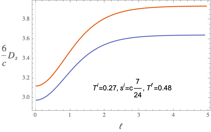
One can convert the restriction set by the QNEC for a fixed initial to a lower and upper bound for the entropy density (temperature) for a fixed final temperature (entropy density) via (5). Substituting these in (10), one readily obtains a lower and an upper bound on for a fixed initial temperature and entropy density, and a fixed final temperature (as shown in Fig. 7) or for a fixed final entropy density. Both the lower and upper bounds increase monotonically with .
References
- Brandão and Gour (2015) F. G. S. L. Brandão and G. Gour, Phys. Rev. Lett. 115, 070503 (2015).
- Guryanova et al. (2016) Y. Guryanova, S. Popescu, A. J. Short, R. Silva, and P. Skrzypczyk, Nature Communications 7 (2016), 10.1038/ncomms12049.
- Yunger Halpern and Renes (2016) N. Yunger Halpern and J. M. Renes, Phys. Rev. E 93, 022126 (2016).
- Yunger Halpern et al. (2016) N. Yunger Halpern, P. Faist, J. Oppenheim, and A. Winter, Nature Communications 7 (2016), 10.1038/ncomms12051.
- Goold et al. (2016) J. Goold, M. Huber, A. Riera, L. d. Rio, and P. Skrzypczyk, Journal of Physics A: Mathematical and Theoretical 49, 143001 (2016).
- Gour et al. (2018) G. Gour, D. Jennings, F. Buscemi, R. Duan, and I. Marvian, Nature Communications 9 (2018), 10.1038/s41467-018-06261-7.
- Chitambar and Gour (2019) E. Chitambar and G. Gour, Rev. Mod. Phys. 91, 025001 (2019).
- Bousso et al. (2016a) R. Bousso, Z. Fisher, S. Leichenauer, and A. C. Wall, Physical Review D 93 (2016a), 10.1103/physrevd.93.064044.
- Bousso et al. (2016b) R. Bousso, Z. Fisher, J. Koeller, S. Leichenauer, and A. C. Wall, Physical Review D 93 (2016b), 10.1103/physrevd.93.024017.
- Malik and Lopez-Mobilia (2020) T. A. Malik and R. Lopez-Mobilia, Phys. Rev. D 101, 066028 (2020), arXiv:1910.07594 [hep-th] .
- Koeller and Leichenauer (2016) J. Koeller and S. Leichenauer, Physical Review D 94 (2016), 10.1103/physrevd.94.024026.
- Balakrishnan et al. (2019) S. Balakrishnan, T. Faulkner, Z. U. Khandker, and H. Wang, JHEP 09, 020 (2019), arXiv:1706.09432 [hep-th] .
- Ceyhan and Faulkner (2020) F. Ceyhan and T. Faulkner, Commun. Math. Phys. 377, 999 (2020), arXiv:1812.04683 [hep-th] .
- Wall (2012) A. C. Wall, Phys. Rev. D 85, 024015 (2012), arXiv:1105.3520 [gr-qc] .
- Leichenauer et al. (2018) S. Leichenauer, A. Levine, and A. Shahbazi-Moghaddam, Phys. Rev. D 98, 086013 (2018), arXiv:1802.02584 [hep-th] .
- Lashkari (2019) N. Lashkari, JHEP 01, 059 (2019), arXiv:1810.09306 [hep-th] .
- Moosa et al. (2021) M. Moosa, P. Rath, and V. P. Su, JHEP 01, 064 (2021), arXiv:2007.15025 [hep-th] .
- Deffner and Lutz (2010) S. Deffner and E. Lutz, Phys. Rev. Lett. 105, 170402 (2010).
- Deffner and Lutz (2011) S. Deffner and E. Lutz, Phys. Rev. Lett. 107, 140404 (2011).
- Plastina et al. (2014) F. Plastina, A. Alecce, T. Apollaro, G. Falcone, G. Francica, F. Galve, N. Lo Gullo, and R. Zambrini, Physical Review Letters 113 (2014), 10.1103/physrevlett.113.260601.
- Angel Garcıa-March et al. (2016) M. Angel Garcıa-March, T. Fogarty, S. Campbell, T. Busch, and M. Paternostro, New Journal of Physics 18, 103035 (2016).
- Van Vu and Hasegawa (2021) T. Van Vu and Y. Hasegawa, Physical Review Letters 127 (2021), 10.1103/physrevlett.127.190601.
- Landi and Paternostro (2021) G. T. Landi and M. Paternostro, Rev. Mod. Phys. 93, 035008 (2021).
- Bardeen et al. (1973) J. M. Bardeen, B. Carter, and S. W. Hawking, Commun. Math. Phys. 31, 161 (1973).
- Balasubramanian et al. (2011) V. Balasubramanian, A. Bernamonti, J. de Boer, N. Copland, B. Craps, E. Keski-Vakkuri, B. Muller, A. Schafer, M. Shigemori, and W. Staessens, Phys. Rev. Lett. 106, 191601 (2011), arXiv:1012.4753 [hep-th] .
- Hubeny and Rangamani (2010) V. E. Hubeny and M. Rangamani, Adv. High Energy Phys. 2010, 297916 (2010), arXiv:1006.3675 [hep-th] .
- Chesler and Yaffe (2014) P. M. Chesler and L. G. Yaffe, JHEP 07, 086 (2014), arXiv:1309.1439 [hep-th] .
- Calabrese and Cardy (2004) P. Calabrese and J. L. Cardy, J. Stat. Mech. 0406, P06002 (2004), arXiv:hep-th/0405152 .
- Calabrese and Cardy (2005) P. Calabrese and J. L. Cardy, J. Stat. Mech. 0504, P04010 (2005), arXiv:cond-mat/0503393 .
- Calabrese and Cardy (2009) P. Calabrese and J. Cardy, J. Phys. A 42, 504005 (2009), arXiv:0905.4013 [cond-mat.stat-mech] .
- Hubeny et al. (2013a) V. E. Hubeny, M. Rangamani, and E. Tonni, JHEP 05, 136 (2013a), arXiv:1302.0853 [hep-th] .
- Liu and Suh (2014a) H. Liu and S. J. Suh, Phys. Rev. Lett. 112, 011601 (2014a), arXiv:1305.7244 [hep-th] .
- Liu and Suh (2014b) H. Liu and S. J. Suh, Phys. Rev. D 89, 066012 (2014b), arXiv:1311.1200 [hep-th] .
- Rangamani et al. (2016) M. Rangamani, M. Rozali, and A. Vincart-Emard, JHEP 04, 069 (2016), arXiv:1512.03478 [hep-th] .
- Leichenauer and Moosa (2015) S. Leichenauer and M. Moosa, Phys. Rev. D 92, 126004 (2015), arXiv:1505.04225 [hep-th] .
- Calabrese and Cardy (2016) P. Calabrese and J. Cardy, J. Stat. Mech. 1606, 064003 (2016), arXiv:1603.02889 [cond-mat.stat-mech] .
- Aharony et al. (2000) O. Aharony, S. S. Gubser, J. M. Maldacena, H. Ooguri, and Y. Oz, Phys. Rept. 323, 183 (2000), arXiv:hep-th/9905111 .
- Brown and Henneaux (1986) J. D. Brown and M. Henneaux, Commun. Math. Phys. 104, 207 (1986).
- Henningson and Skenderis (1998) M. Henningson and K. Skenderis, JHEP 07, 023 (1998), arXiv:hep-th/9806087 .
- Balasubramanian and Kraus (1999) V. Balasubramanian and P. Kraus, Commun. Math. Phys. 208, 413 (1999), arXiv:hep-th/9902121 .
- Sfetsos (1995) K. Sfetsos, Nucl. Phys. B 436, 721 (1995), arXiv:hep-th/9408169 .
- Banados et al. (1992) M. Banados, C. Teitelboim, and J. Zanelli, Phys. Rev. Lett. 69, 1849 (1992), arXiv:hep-th/9204099 .
- Banados et al. (1993) M. Banados, M. Henneaux, C. Teitelboim, and J. Zanelli, Phys. Rev. D 48, 1506 (1993), [Erratum: Phys.Rev.D 88, 069902 (2013)], arXiv:gr-qc/9302012 .
- Ryu and Takayanagi (2006) S. Ryu and T. Takayanagi, Phys. Rev. Lett. 96, 181602 (2006), arXiv:hep-th/0603001 .
- Hubeny et al. (2007) V. E. Hubeny, M. Rangamani, and T. Takayanagi, JHEP 07, 062 (2007), arXiv:0705.0016 [hep-th] .
- (46) This computation can be readily done by the geodetic distance formula between two end points and in the Poincaré patch metric. This geodetic distance is simply where with .
- Holzhey et al. (1994) C. Holzhey, F. Larsen, and F. Wilczek, Nucl. Phys. B 424, 443 (1994), arXiv:hep-th/9403108 .
- Cadoni and Melis (2010) M. Cadoni and M. Melis, Found. Phys. 40, 638 (2010), arXiv:0907.1559 [hep-th] .
- Unanyan et al. (2010) R. G. Unanyan, D. Muth, and M. Fleischhauer, Phys. Rev. A 81, 022119 (2010), arXiv:0910.3868 [quant-ph] .
- Unanyan and Fleischhauer (2014) R. G. Unanyan and M. Fleischhauer, Phys. Rev. A 89, 062330 (2014), arXiv:1011.4838 [quant-ph] .
- Asplund et al. (2015) C. T. Asplund, A. Bernamonti, F. Galli, and T. Hartman, JHEP 09, 110 (2015), arXiv:1506.03772 [hep-th] .
- von Keyserlingk et al. (2018) C. von Keyserlingk, T. Rakovszky, F. Pollmann, and S. Sondhi, Phys. Rev. X 8, 021013 (2018), arXiv:1705.08910 [cond-mat.str-el] .
- Mezei and Stanford (2017) M. Mezei and D. Stanford, JHEP 05, 065 (2017), arXiv:1608.05101 [hep-th] .
- Hubeny et al. (2013b) V. E. Hubeny, H. Maxfield, M. Rangamani, and E. Tonni, JHEP 08, 092 (2013b), arXiv:1306.4004 [hep-th] .
- Kudler-Flam (2021) J. Kudler-Flam, Phys. Rev. Lett. 126, 171603 (2021), arXiv:2102.05053 [hep-th] .
- Kudler-Flam et al. (2021) J. Kudler-Flam, V. Narovlansky, and S. Ryu, (2021), arXiv:2108.00011 [hep-th] .
- Mandal et al. (2015) G. Mandal, R. Sinha, and N. Sorokhaibam, JHEP 01, 036 (2015), arXiv:1405.6695 [hep-th] .
- Erdmenger et al. (2017) J. Erdmenger, D. Fernandez, M. Flory, E. Megias, A.-K. Straub, and P. Witkowski, JHEP 10, 034 (2017), arXiv:1705.04696 [hep-th] .
- Kim and Huse (2013) H. Kim and D. A. Huse, Phys. Rev. Lett. 111, 127205 (2013), arXiv:1306.4306 [quant-ph] .
- Carleo et al. (2014) G. Carleo, F. Becca, L. Sanchez-Palencia, S. Sorella, and M. Fabrizio, Phys. Rev. A 89, 031602 (2014), arXiv:1310.2246 [cond-mat.quant-gas] .
- Eisert et al. (2013) J. Eisert, M. van den Worm, S. R. Manmana, and M. Kastner, Phys. Rev. Lett. 111, 260401 (2013).
- Hauke and Tagliacozzo (2013) P. Hauke and L. Tagliacozzo, Phys. Rev. Lett. 111, 207202 (2013).
- Chiara et al. (2006) G. D. Chiara, S. Montangero, P. Calabrese, and R. Fazio, Journal of Statistical Mechanics: Theory and Experiment 2006, P03001 (2006).
- Cheneau et al. (2012) M. Cheneau, P. Barmettler, D. Poletti, M. Endres, P. Schauß, T. Fukuhara, C. Gross, I. Bloch, C. Kollath, and S. Kuhr, Nature 481, 484 (2012).
- Langen et al. (2013) T. Langen, R. Geiger, M. Kuhnert, B. Rauer, and J. Schmiedmayer, Nature Physics 9, 640 (2013).
- Jurcevic et al. (2014) P. Jurcevic, B. P. Lanyon, P. Hauke, C. Hempel, P. Zoller, R. Blatt, and C. F. Roos, Nature 511, 202–205 (2014).
- Richerme et al. (2014) P. Richerme, Z.-X. Gong, A. Lee, C. Senko, J. Smith, M. Foss-Feig, S. Michalakis, A. V. Gorshkov, and C. Monroe, Nature 511, 198–201 (2014).
- Bonnes et al. (2014) L. Bonnes, F. H. Essler, and A. M. Läuchli, Physical Review Letters 113 (2014), 10.1103/physrevlett.113.187203.
- Hartman and Maldacena (2013) T. Hartman and J. Maldacena, JHEP 05, 014 (2013), arXiv:1303.1080 [hep-th] .
- Ecker et al. (2019) C. Ecker, D. Grumiller, W. van der Schee, M. Sheikh-Jabbari, and P. Stanzer, SciPost Phys. 6, 036 (2019), arXiv:1901.04499 [hep-th] .
- Casini et al. (2017) H. Casini, E. Teste, and G. Torroba, J. Phys. A 50, 364001 (2017), arXiv:1703.10656 [hep-th] .
- Bekenstein (1981) J. D. Bekenstein, Phys. Rev. Lett. 46, 623 (1981).
- Buchel et al. (2013) A. Buchel, R. C. Myers, and A. van Niekerk, Phys. Rev. Lett. 111, 201602 (2013), arXiv:1307.4740 [hep-th] .
- Banados (1999) M. Banados, AIP Conf. Proc. 484, 147 (1999), arXiv:hep-th/9901148 .
- Banerjee et al. (2022) A. Banerjee, T. Kibe, N. Mittal, A. Mukhopadhyay, and P. Roy, (2022), arXiv:2202.00022 [hep-th] .
- Sagawa (2017) T. Sagawa, “Second law, entropy production, and reversibility in thermodynamics of information,” (2017), arXiv:1712.06858 [cond-mat.stat-mech] .
- Esposito et al. (2010) M. Esposito, K. Lindenberg, and C. Van den Broeck, New Journal of Physics 12, 013013 (2010).
- Reeb and Wolf (2014) D. Reeb and M. M. Wolf, New Journal of Physics 16, 103011 (2014).
- Compère et al. (2016) G. Compère, P. Mao, A. Seraj, and M. M. Sheikh-Jabbari, JHEP 01, 080 (2016), arXiv:1511.06079 [hep-th] .
- Sheikh-Jabbari and Yavartanoo (2016) M. M. Sheikh-Jabbari and H. Yavartanoo, Eur. Phys. J. C 76, 493 (2016), arXiv:1603.05272 [hep-th] .
- Banerjee et al. (2016) S. Banerjee, T. Ishii, L. K. Joshi, A. Mukhopadhyay, and P. Ramadevi, JHEP 08, 048 (2016), arXiv:1603.06935 [hep-th] .