ApproxIFER: A Model-Agnostic Approach to Resilient and Robust Prediction Serving Systems

Machine learning as a service (MLaS) paradigms allow incapable clients to outsource their computationally-demanding tasks such as neural network inference tasks to powerful clouds [1, 2, 3, 4]. More specifically, prediction serving systems host complex machine learning models and respond to the inference queries of the clients by the corresponding predictions with low latency. To ensure a fast response to the different queries in the presence of stragglers, prediction serving systems distribute these queries on multiple worker nodes in the system each having an instance of the deployed model [5]. Such systems often mitigate stragglers through replication which assigns the same task to multiple workers, either proactively or reactively, in order to reduce the tail latency of the computations [6, 7, 8, 9, 10, 11, 12]. Replication-based systems, however, entail significant overhead as a result of assigning the same task to multiple workers.

Erasure coding is known to be more resource-efficient compared to replication and has been recently leveraged to speed up distributed computing and learning systems [13, 14, 15, 16, 17, 18, 19]. The traditional coding-theoretic approaches, known as the coded computing approaches, are usually limited to polynomial computations and require a large number of workers that depends on the desired computation. Hence, such techniques cannot be directly applied in prediction serving systems.

To overcome the limitations of the traditional coding-theoretic approaches, a learning-based approach known as ParM has been proposed in [20]. In this approach, the prediction queries are first encoded using an erasure code. These coded queries are then transformed into coded predictions by learning parity models to provide straggler resiliency. The desired predictions can be then reconstructed from the fastest workers as shown in Fig. 1. By doing this, ParM can be applied to non-polynomial computations with a number of workers that is independent of the computations.

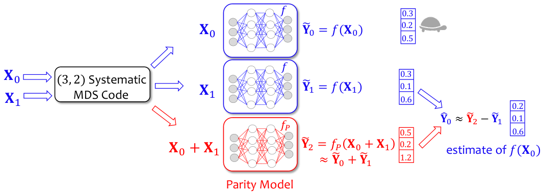
These parity models, however, depend on the model hosted by the cloud and are suitable for tolerating one straggler and handling a small number of queries (typically less than $4$). Moreover, they require retraining whenever they are used with a new cloud model. In this work, we take a different approach leveraging approximate coded computing techniques [21] to design scalable, straggler-resilient and Byzantine-robust prediction serving systems. Our approach relies on rational interpolation techniques [22] to estimate the predictions of the slow and erroneous workers from the predictions of the other workers. Our contributions in this work are summarized as follows.

1. 1.

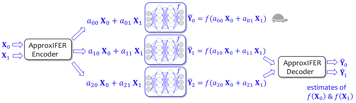
   We propose ApproxIFER, a model-agnostic inference framework that leverages approximate computing techniques. In ApproxIFER, all workers deploy instances of the model hosted by the cloud and no additional models are required as shown in Fig. 2. Furthermore, the encoding and the decoding procedures of ApproxIFER do not depend on the model depolyed by the cloud. This enables ApproxIFER to be easily applied to any neural network architecture.

2. 2.

   ApproxIFER is also robust to erroneous workers that return incorrect predictions either unintentionally or adversarially. To do so, we have proposed an algebraic interpolation algorithm to decode the desired predictions from the erroneous coded predictions.
   ApproxIFER requires a significantly smaller number of workers than the conventional replication method. More specifically, to tolerate $E$ Byzantine adversarial workers, ApproxIFER requires only $2K+2E$ workers whereas the replication-based schemes require $(2E+1)K$ workers. Moreover, ApproxIFER can be set to tolerate any number of stragglers $S$ and errors $E$ efficiently while scaling well with the number of queries $K$, whereas the prior works focused on the case where $S=1,E=0$ and $K=2,3,4$.

3. 3.

   We run extensive experiments on MNIST, Fashion-MNIST, and CIFAR-$10$ datasets on VGG, ResNet, DenseNet, and GoogLeNet architectures which show that ApproxIFER improves the prediction accuracy by up to $58\%$ compared to the prior approaches for large $K$. The results of one of our experiments on ResNet are shown in Fig. 3, but we later report extensive experiments on those datasets and architectures showing a consistent significant accuracy improvement over the prior works.

Organization. The rest of this paper is organized as follows. We describe the problem setting in Section 2. Then, we describe ApproxIFER in Section 3. In Section 4, we present our extensive experimental results. In Section 5, we discuss the closely-related works. Finally, we discuss some concluding remarks and the future research directions in Section 6.

System Architecture. We consider a prediction serving system with $N+1$ workers. The prediction serving system is hosting a machine learning model denoted by $f$. We refer to this model as the hosted or the deployed model. Unlike ParM [20], all workers have the same model $f$ in our work as shown in Fig. 4.

The input queries are grouped such that each group has $K$ queries. We denote the set of $K$ queries in a group by $\mathbf{X}_{0},\mathbf{X}_{1},\cdots,\mathbf{X}_{K-1}$.

Goal. The goal is to compute the predictions $\mathbf{Y}_{0}=f(\mathbf{X}_{0}),\mathbf{Y}_{1}=f(\mathbf{X}_{1}),\cdots,\mathbf{Y}_{K-1}=f(\mathbf{X}_{K-1})$ while being resilient to any $S$ stragglers and robust to any $E$ Byzantine workers.

In this section, we present our proposed protocol based on leveraging approximate coded computing. The encoder and the decoder of ApproxIFER are based on rational functions and rational interpolation. Most coding-theoretic approaches for designing straggler-resilient and Byzantine-robust distributed systems rely on polynomial encoders and polynomial interpolation for decoding. Polynomial interpolation, however, is known to be unstable [23]. On the other hand, rational interpolation is known to be extremely stable and can lead to faster convergence compared to polynomial interpolation [22]. This motivated a recent work to leverage rational functions rather than polynomials to design straggler-resilient distributed training algorithms [21]. ApproxIFER also leverages rational functions and rational interpolation. We provide a very brief background about rational functions next.

Rational Interpolation Background. Consider a function $f$, $n+1$ distinct points $a\leq x_{0}<x_{1},\cdots<x_{n}\leq b$ and the corresponding evaluations of $f$ at these points denoted by $f_{0},f_{1},\cdots,f_{n-1},f_{n}$. Berrut’s rational interpolant of $f$ is then defined as follows [22]:

$\displaystyle r(x)\mbox{$\stackrel{{\scriptstyle\rm def}}{{=}}$}\sum\limits_{i=0}^{n}f_{i}\ell_{i}(x),$

(1)

where $\ell_{i}(x)$, for $i\in[n]$, where $[n]\,\mbox{$\stackrel{{\scriptstyle\rm def}}{{=}}$}\,\{0,1,2,\dots,n\}$, are the basis functions defined as follows

$\displaystyle\ell_{i}(x)\mbox{$\stackrel{{\scriptstyle\rm def}}{{=}}$}\frac{(-1)^{i}}{(x-x_{i})}\big/\sum\limits_{i=0}^{n}\frac{(-1)^{i}}{(x-x_{i})},$

(2)

for $i\in[n]$. Berrut’s rational interpolant has several useful properties as it has no pole on the real line [22] and it is extremely well-conditioned [24, 25]. It also converges with rate $O(h)$, where $h\mbox{$\stackrel{{\scriptstyle\rm def}}{{=}}$}\max\limits_{0\leq i\leq n-1}x_{i+1}-x_{i}$ [26].

Rational Interpolation with Erroneous Evaluations. We now provide our proposed error-locator algorithm for rational interpolation in the presence of Byzantine errors. All the details on how this method works along with the theoretical guarantee and proofs are moved to the Appendix A due to space limitations. Let $A_{\text{avl}}$ denote the set of indices corresponding to $N-S+1$ available evaluations of $r(x)$ over $x_{i}$’s, for some $S\geq 1$ that denote the number of stragglers in the context of our system model. Let $A_{\text{adv}}$, with $|A_{\text{adv}}|\leq E$, denote the set of indices corresponding to erroneous evaluations. For $i\in A_{\text{avl}}$, let also $y_{i}$ denote the available and possibly erroneous evaluation of $r(x)$ at $x_{i}$. Then we have $y_{i}=r(x_{i})$, for at least $N-S-E+1$ indices $i\in A_{\text{avl}}$. The proposed algorithm is mainly inspired by the well-known Berlekamp–Welch (BW) decoding algorithm for Reed-Solomon codes in coding theory [27]. We tailor the BW algorithm to get a practical algorithm for rational functions that overcomes the numerical issues arising from inevitable round-off errors in the implementation. This algorithm is provided below.

Note that the equations in Step 1 of Algorithm 1 form a homogeneous system of linear equations with $2(K+E)$ unknown variables where the number of equations is $N-S+1$. In order to guarantee the existence of a non-trivial solution, we must have

$$N\geq 2K+2E+S-1.$$

(3)

This guarantees the existence of a solution to $P(x)$ and $Q(x)$.

Next, the encoding and decoding algorithms of ApproxIFER are discussed in detail.

ApproxIFER Encoding. The $K$ input queries $\mathbf{X}_{j}$, for $j\in[K-1]$, are first encoded into $N+1$ coded queries, denoted by $\tilde{\mathbf{X}}_{i}$, for $i\in[N]$, each given to a worker. As mentioned earlier, the aim is to provide resilience against any $S$ straggler workers and robustness against any $E$ Byzantine adversarial workers. When $E=0$, we assume that $N=K+S-1$ which corresponds to an overhead of $\frac{K+S}{K}$. Otherwise, $N=2(K+E)+S-1$ which corresponds to an overhead of $\frac{2(K+E)+S}{K}$. In general, the overhead is defined as the number of workers divided by the number of queries.

To encode the queries, we leverage Berrut’s rational interpolant discussed as follows. First, a rational function $u$ is computed in such a way that it passes through the queries. More specifically,

$\displaystyle u(z)=\sum\limits_{j\in[K-1]}\mathbf{X}_{j}\ell_{j}(z),$

(4)

where $\ell_{j}(x)$, for $j\in[K-1]$, are the basis functions defined as follows

$\displaystyle\ell_{j}(z)=\frac{(-1)^{j}}{(z-\alpha_{j})}\big/\sum\limits_{j\in[K-1]}\frac{(-1)^{j}}{(z-\alpha_{j})},$

(5)

and $\alpha_{j}$ is selected as a Chebyshev point of the first kind as

$\displaystyle\alpha_{j}=\cos\frac{(2j+1)\pi}{2K}$

(6)

for all $j\in[K-1].$ The queries are then encoded using this rational function as follows

$\displaystyle\tilde{\mathbf{X}}_{i}\mbox{$\stackrel{{\scriptstyle\rm def}}{{=}}$}u(\beta_{i}),$

(7)

where $\beta_{i}$ is selected as a Chebyshev point of the second kind as follows

$\displaystyle\beta_{i}=\cos\frac{i\pi}{N},$

(8)

for $i\in[N]$. The $i$-th worker is then required to compute the prediction on the coded query $\tilde{\mathbf{X}}_{i}$. That is, the $i$-th worker computes

$\displaystyle\tilde{\mathbf{Y}}_{i}\mbox{$\stackrel{{\scriptstyle\rm def}}{{=}}$}f(\tilde{\mathbf{X}}_{i})=f(u(\beta_{i})),$

(9)

where $i\in[N]$.

ApproxIFER Decoding. When $E=0$, the decoder waits for the results of the fastest $K$ workers before decoding. Otherwise, in the presence of Byzantine workers, i.e., $E>0$, the decoder waits for the results of the fastest $2(K+E)$ workers. After receiving the sufficient number of coded predictions, the decoding approach proceeds with the following two steps.

1. 1.

   Locating Adversarial Workers. In presence of Byzantine workers that return erroneous predictions aiming at altering the inference results or even unintentionally, we utilize Algorithm 2 provided below to locate them. The predictions corresponding to these workers can be then excluded in the decoding step. Algorithm 2 runs our proposed error-locator algorithm for rational interpolation in presence of errors provided in Algorithm 1 several times, each time associated to one of the soft labels in the predictions on the coded queries, i.e., $f(\tilde{\mathbf{X}}_{i})$’s. At the end, we decide the error locations based on a majority vote on all estimates of the error locations. In Algorithm 2, $f_{j}(\tilde{\mathbf{X}}_{i})$ denotes the $j$’th coordinate of $f(\tilde{\mathbf{X}}_{i})$ which is the soft label corresponding to class $j$ in the prediction on the coded query $f(\tilde{\mathbf{X}}_{i})$. Also, $C$ denotes the total number of classes which is equal to the size of $f(\tilde{\mathbf{X}}_{i})$’s.

   Input: $f(\tilde{\mathbf{X}}_{i})$’s for $i\in A_{\text{avl}}$, $\beta_{i}$’s as specified in (8), $K$, C and $E$.
   Output: The set of indices $A_{\text{adv}}$ corresponding to malicious workers.
   
   Set $\mathbf{I}=[\mathbf{0}]_{C\times E}.$

   For $j=1,\cdots,C$
   

   Step 1: Set $P(x)\mbox{$\stackrel{{\scriptstyle\rm def}}{{=}}$}\sum\limits_{j=0}^{K+E-1}P_{j}x^{j},$ and $Q(x)\mbox{$\stackrel{{\scriptstyle\rm def}}{{=}}$}\sum\limits_{j=1}^{K+E-1}Q_{j}x^{j}+1.$

   Step 2: Solve the system of linear equations provided by

   $$P(\beta_{i})=f_{j}(\tilde{\mathbf{X}}_{i})Q(\beta_{i}),\quad\quad\forall i\in A_{\text{avl}}.$$

   to find the coefficients $P_{j}$’s and $Q_{j}$’s.

   Step 3: Set $a_{i}=Q(\beta_{i})$, $\forall i\in A_{\text{avl}}$.

   Step 4: Sort $a_{i}$’s increasingly with respect to their absolute values, i.e., $|a_{i_{1}}|\leq\cdots\leq|a_{i_{N-S+1}}|$.

   Step 5: Set $\mathbf{I}[j,:]=[i_{1},\cdots,i_{E}].$

   end

   Return: $A_{\text{adv}}$: The set of $E$ most-frequent elements of $\mathbf{I}$.

2. 2.

   Decoding. After excluding the erroneous workers, the approximate predictions can be then recovered from the results of the workers who returned correct coded predictions whose indices are denoted by $\mathcal{F}$. Specifically, a rational function $r$ is first constructed as follows

   $\displaystyle r(z)=\frac{1}{\sum\limits_{i\in\mathcal{F}}\frac{(-1)^{i}}{(z-\beta_{i})}}\sum\limits_{i\in\mathcal{F}}\frac{(-1)^{i}}{(z-\beta_{i})}f(\tilde{\mathbf{X}}_{i}),$

   (10)

   where $|\mathcal{F}|=K$ when $E=0$ and $|\mathcal{F}|=2K+E$ otherwise.

   The approximate predictions denoted by $\hat{\mathbf{Y}}_{0},\cdots,\hat{\mathbf{Y}}_{K-1}$ then are recovered as follows

   $\displaystyle\hat{\mathbf{Y}}_{j}=r(\alpha_{j}),$

   (11)

   for all $j\in[K-1]$.

In this section, we present several experiments to show the effectiveness of ApproxIFER.

Replication is the most widely used technique for providing straggler resiliency and Byzantine robustness in distributed systems. In this technique, the same task is assigned to multiple workers either proactively or reactively. In the proactive approaches, to tolerate $S$ stragglers, the same task is assigned to $S+1$ workers before starting the computation. While such approaches reduce the latency significantly, they incur significant overhead. The reactive approaches [36, 9] avoid such overhead by assigning the same task to other workers only after a deadline is passed as in Hadoop MapReduce [7]. This approach also incurs a significant latency cost as it has to wait before reassigning the tasks.

Recently, coding-theoretic approaches have shown great success in mitigating stragglers in distributed computing and machine learning [13, 37, 16, 38, 39, 19, 40, 14, 41]. Such ideas have also been extended to not only provide straggler resiliency, but also Byzantine robustness and data privacy. Specifically, the coded computing paradigm has recently emerged by adapting erasure coding based ideas to design straggler-resilient, Byzantine-robust and private distributed computing systems often involving polynomial-type computations [42, 15, 43, 44, 45, 46, 47, 48]. However, many applications involve non-polynomial computations such as distributed training and inference of neural networks.

A natural approach to get around the polynomial limitation is to approximate any non-polynomial computations. This idea has been leveraged to train a logistic regression model in [46]. This approximation approach, however, is not suitable for neural networks as the number of workers needed is proportional to the degree of the function being computed and also the number of queries. Motivated by mitigating these limitations, a learning-based approach was proposed in [20] to tackle these challenges in prediction serving systems. This idea provides the same straggler-resilience as that of the underlying erasure code, and hence decouples the straggler-resilience guarantee from the computation carried out by the system. This is achieved by learning a parity model known as ParM that transforms the coded queries to coded predictions.

As we discussed, the learning-based approaches do not scale well. This motivates us in this work to explore a different approach based on approximate coded computing [49, 21]. Approximate computing was leveraged before in distributed matrix-matrix multiplication in [50]. Moreover, an approximate coded computing approach was developed in [49] for distributed matrix-matrix multiplication. More recently, a numerically stable straggler-resilient approximate coded computing approach has been developed in [21]. In particular, this approach is not restricted to polynomials and can be used to approximately compute arbitrary functions unlike the conventional coded computing techniques. One of the key features of this approach is that it uses rational functions [51] rather than polynomials to introduce coded redundancy which are known to be numerically stable. This approach, however, does not provide robustness against Byzantine workers. Finally, this approach has been leveraged in distributed training of LeNet-$5$ using MNIST dataset [29] and resulted in an accuracy that is comparable to the replication-based strategy.

In this work, we have introduced ApproxIFER, a model-agnostic straggler-resilient, and Byzantine-robust framework for prediction serving systems. The key idea of ApproxIFER is that it encodes the queries carefully such that the desired predictions can be recovered efficiently in the presence of both stragglers and Byzantine workers. Unlike the learning-based approaches, our approach does not require training any parity models, can be set to tolerate any number of stragglers and Byzantine workers efficiently. Our experiments on the MNIST, the Fashion-MNIST and the CIFAR-$10$ datasets on various architectures such as VGG, ResNet, DenseNet, and GoogLeNet show that ApproxIFER improves the prediction accuracy by up to $58\%$ compared to the learning-based approaches. An interesting future direction is to extend ApproxIFER to be preserve the privacy of data.

References

- [1] Amazon AWS AI. https://aws.amazon.com/machine-learning/. Last accessed: May 2021.
- [2] Azure Machine Learning Studio. https://azure.microsoft.com/en-us/services/machine-learning-studio/. Last accessed: May 2021.
- [3] Google Cloud AI. https://cloud.google.com/products/machine-learning/. Last accessed: May 2021.
- [4] Christopher Olston, Noah Fiedel, Kiril Gorovoy, Jeremiah Harmsen, Li Lao, Fangwei Li, Vinu Rajashekhar, Sukriti Ramesh, and Jordan Soyke. Tensorflow-serving: Flexible, high-performance ml serving. arXiv preprint arXiv:1712.06139, 2017.
- [5] Daniel Crankshaw, Xin Wang, Guilio Zhou, Michael J Franklin, Joseph E Gonzalez, and Ion Stoica. Clipper: A low-latency online prediction serving system. In 14th USENIX Symposium on Networked Systems Design and Implementation (NSDI 17), pages 613–627, 2017.
- [6] Lalith Suresh, Marco Canini, Stefan Schmid, and Anja Feldmann. C3: Cutting tail latency in cloud data stores via adaptive replica selection. In 12th USENIX Symposium on Networked Systems Design and Implementation (NSDI 15), pages 513–527, 2015.
- [7] Apache Hadoop. http://hadoop.apache.org/. Last accessed: May 2021.
- [8] Ganesh Ananthanarayanan, Ali Ghodsi, Scott Shenker, and Ion Stoica. Effective straggler mitigation: Attack of the clones. In 10th USENIX Symposium on Networked Systems Design and Implementation (NSDI 13), pages 185–198, 2013.
- [9] Jeffrey Dean and Luiz André Barroso. The tail at scale. Communications of the ACM, 56(2):74–80, 2013.
- [10] Nihar B Shah, Kangwook Lee, and Kannan Ramchandran. When do redundant requests reduce latency? IEEE Transactions on Communications, 64(2):715–722, 2015.
- [11] Kristen Gardner, Samuel Zbarsky, Sherwin Doroudi, Mor Harchol-Balter, and Esa Hyytia. Reducing latency via redundant requests: Exact analysis. ACM SIGMETRICS Performance Evaluation Review, 43(1):347–360, 2015.
- [12] Manmohan Chaubey and Erik Saule. Replicated data placement for uncertain scheduling. In 2015 IEEE International Parallel and Distributed Processing Symposium Workshop, pages 464–472. IEEE, 2015.
- [13] Kangwook Lee, Maximilian Lam, Ramtin Pedarsani, Dimitris Papailiopoulos, and Kannan Ramchandran. Speeding up distributed machine learning using codes. IEEE Transactions on Information Theory, 64(3):1514–1529, 2017.
- [14] Sanghamitra Dutta, Viveck Cadambe, and Pulkit Grover. " short-dot" computing large linear transforms distributedly using coded short dot products. In Proceedings of the 30th International Conference on Neural Information Processing Systems, pages 2100–2108, 2016.
- [15] Qian Yu, Songze Li, Netanel Raviv, Seyed Mohammadreza Mousavi Kalan, Mahdi Soltanolkotabi, and Salman A Avestimehr. Lagrange coded computing: Optimal design for resiliency, security, and privacy. In The 22nd International Conference on Artificial Intelligence and Statistics, pages 1215–1225. PMLR, 2019.
- [16] Qian Yu, Mohammad Ali Maddah-Ali, and A Salman Avestimehr. Polynomial codes: an optimal design for high-dimensional coded matrix multiplication. In Proceedings of the 31st International Conference on Neural Information Processing Systems, pages 4406–4416, 2017.
- [17] Krishna Giri Narra, Zhifeng Lin, Mehrdad Kiamari, Salman Avestimehr, and Murali Annavaram. Slack squeeze coded computing for adaptive straggler mitigation. In Proceedings of the International Conference for High Performance Computing, Networking, Storage and Analysis, pages 1–16, 2019.
- [18] Nikhil Krishnan Muralee Krishnan, Seyederfan Hosseini, and Ashish Khisti. Coded sequential matrix multiplication for straggler mitigation. Advances in Neural Information Processing Systems, 33, 2020.
- [19] Pedro Soto, Jun Li, and Xiaodi Fan. Dual entangled polynomial code: Three-dimensional coding for distributed matrix multiplication. In International Conference on Machine Learning, pages 5937–5945. PMLR, 2019.
- [20] Jack Kosaian, KV Rashmi, and Shivaram Venkataraman. Parity models: erasure-coded resilience for prediction serving systems. In Proceedings of the 27th ACM Symposium on Operating Systems Principles, pages 30–46, 2019.
- [21] Tayyebeh Jahani-Nezhad and Mohammad Ali Maddah-Ali. Berrut approximated coded computing: Straggler resistance beyond polynomial computing. arXiv preprint arXiv:2009.08327, 2020.
- [22] J-P Berrut. Rational functions for guaranteed and experimentally well-conditioned global interpolation. Computers & Mathematics with Applications, 15(1):1–16, 1988.
- [23] Jean-Paul Berrut and Georges Klein. Recent advances in linear barycentric rational interpolation. Journal of Computational and Applied Mathematics, 259:95–107, 2014.
- [24] Len Bos, Stefano De Marchi, and Kai Hormann. On the lebesgue constant of berrut’s rational interpolant at equidistant nodes. Journal of Computational and Applied Mathematics, 236(4):504–510, 2011.
- [25] Len Bos, Stefano De Marchi, Kai Hormann, and Jean Sidon. Bounding the lebesgue constant for berrut’s rational interpolant at general nodes. Journal of Approximation Theory, 169:7–22, 2013.
- [26] Michael S Floater and Kai Hormann. Barycentric rational interpolation with no poles and high rates of approximation. Numerische Mathematik, 107(2):315–331, 2007.
- [27] Richard E Blahut. Algebraic codes on lines, planes, and curves: an engineering approach. Cambridge University Press, 2008.
- [28] Adam Paszke, Sam Gross, Francisco Massa, Adam Lerer, James Bradbury, Gregory Chanan, Trevor Killeen, Zeming Lin, Natalia Gimelshein, Luca Antiga, et al. Pytorch: An imperative style, high-performance deep learning library. In NeurIPS, 2019.
- [29] Yann LeCun, Léon Bottou, Yoshua Bengio, and Patrick Haffner. Gradient-based learning applied to document recognition. Proceedings of the IEEE, 86(11):2278–2324, 1998.
- [30] Han Xiao, Kashif Rasul, and Roland Vollgraf. Fashion-mnist: a novel image dataset for benchmarking machine learning algorithms. arXiv preprint arXiv:1708.07747, 2017.
- [31] Alex Krizhevsky, Geoffrey Hinton, et al. Learning multiple layers of features from tiny images. 2009.
- [32] Karen Simonyan and Andrew Zisserman. Very deep convolutional networks for large-scale image recognition. arXiv preprint arXiv:1409.1556, 2014.
- [33] Gao Huang, Zhuang Liu, Laurens Van Der Maaten, and Kilian Q Weinberger. Densely connected convolutional networks. In Proceedings of the IEEE conference on computer vision and pattern recognition, pages 4700–4708, 2017.
- [34] Kaiming He, Xiangyu Zhang, Shaoqing Ren, and Jian Sun. Deep residual learning for image recognition. In Proceedings of the IEEE conference on computer vision and pattern recognition, pages 770–778, 2016.
- [35] Christian Szegedy, Wei Liu, Yangqing Jia, Pierre Sermanet, Scott Reed, Dragomir Anguelov, Dumitru Erhan, Vincent Vanhoucke, and Andrew Rabinovich. Going deeper with convolutions. In Proceedings of the IEEE conference on computer vision and pattern recognition, pages 1–9, 2015.
- [36] Matei Zaharia, Andy Konwinski, Anthony D Joseph, Randy H Katz, and Ion Stoica. Improving mapreduce performance in heterogeneous environments. In Osdi, volume 8, page 7, 2008.
- [37] Rashish Tandon, Qi Lei, Alexandros G Dimakis, and Nikos Karampatziakis. Gradient coding: Avoiding stragglers in distributed learning. In International Conference on Machine Learning, pages 3368–3376. PMLR, 2017.
- [38] Min Ye and Emmanuel Abbe. Communication-computation efficient gradient coding. In International Conference on Machine Learning, pages 5610–5619. PMLR, 2018.
- [39] Hongyi Wang, Zachary Charles, and Dimitris Papailiopoulos. Erasurehead: Distributed gradient descent without delays using approximate gradient coding. arXiv preprint arXiv:1901.09671, 2019.
- [40] Hema Venkata Krishna Giri Narra, Zhifeng Lin, Ganesh Ananthanarayanan, Salman Avestimehr, and Murali Annavaram. Collage inference: Using coded redundancy for lowering latency variation in distributed image classification systems. In 2020 IEEE 40th International Conference on Distributed Computing Systems (ICDCS), pages 453–463. IEEE, 2020.
- [41] Sinong Wang, Jiashang Liu, and Ness Shroff. Fundamental limits of approximate gradient coding. Proceedings of the ACM on Measurement and Analysis of Computing Systems, 3(3):1–22, 2019.
- [42] Yaoqing Yang, Pulkit Grover, and Soummya Kar. Coded distributed computing for inverse problems. In Proceedings of the 31st International Conference on Neural Information Processing Systems, pages 709–719, 2017.
- [43] Adarsh M Subramaniam, Anoosheh Heidarzadeh, and Krishna R Narayanan. Collaborative decoding of polynomial codes for distributed computation. In 2019 IEEE Information Theory Workshop (ITW), pages 1–5. IEEE, 2019.
- [44] Mahdi Soleymani, Ramy E. Ali, Hessam Mahdavifar, and A Salman Avestimehr. List-decodable coded computing: Breaking the adversarial toleration barrier. arXiv preprint arXiv:2101.11653, 2021.
- [45] Tingting Tang, Ramy E. Ali, Hanieh Hashemi, Tynan Gangwani, Salman Avestimehr, and Murali Annavaram. Verifiable coded computing: Towards fast, secure and private distributed machine learning. arXiv preprint arXiv:2107.12958, 2021.
- [46] Jinhyun So, Basak Guler, and Salman Avestimehr. A scalable approach for privacy-preserving collaborative machine learning. Advances in Neural Information Processing Systems, 33, 2020.
- [47] Jy-yong Sohn, Dong-Jun Han, Beongjun Choi, and Jaekyun Moon. Election coding for distributed learning: Protecting signsgd against byzantine attacks. Advances in Neural Information Processing Systems, 33, 2020.
- [48] Ankur Mallick, Malhar Chaudhari, and Gauri Joshi. Fast and efficient distributed matrix-vector multiplication using rateless fountain codes. In ICASSP 2019-2019 IEEE International Conference on Acoustics, Speech and Signal Processing (ICASSP), pages 8192–8196. IEEE, 2019.
- [49] Tayyebeh Jahani-Nezhad and Mohammad Ali Maddah-Ali. Codedsketch: A coding scheme for distributed computation of approximated matrix multiplication. IEEE Transactions on Information Theory, 2021.
- [50] Vipul Gupta, Shusen Wang, Thomas Courtade, and Kannan Ramchandran. Oversketch: Approximate matrix multiplication for the cloud. In 2018 IEEE International Conference on Big Data (Big Data), pages 298–304. IEEE, 2018.
- [51] Jean-Paul Berrut and Lloyd N Trefethen. Barycentric lagrange interpolation. SIAM review, 46(3):501–517, 2004.
- [52] Brice Boyer and Erich L Kaltofen. Numerical linear system solving with parametric entries by error correction. In Proceedings of the 2014 Symposium on Symbolic-Numeric Computation, pages 33–38, 2014.
- [53] Erich Kaltofen and Clément Pernet. Cauchy interpolation with errors in the values. Submitted manuscript, 13, 2013.
- [54] Simon R Blackburn. Fast rational interpolation, reed-solomon decoding, and the linear complexity profiles of sequences. IEEE Transactions on Information Theory, 43(2):537–548, 1997.
Appendix A Rational Interpolation in the Presence of Errors
In this section, we provide an algebraic method to interpolate a rational function using its evaluations where some of them are erroneous. Let denote the set of indices corresponding to erroneous evaluations and . The proposed algorithm is mainly inspired by the well-known Berlekamp–Welch (BW) decoding algorithm for Reed-Solomon codes in coding theory [27]. This algorithm enables polynomial interpolation in the presence of erroneous evaluations. Our proposed algorithm extends the BW algorithm to rational functions. Extending the BW algorithm to interpolate rational functions in presence of erroneous evaluations has been studied in the literature, e.g., see [52, 53, 54]. However, we propose a simple yet powerful algorithm that guarantees successful recovery under a slightly different conditions. It is worth noting that no assumption is made on the distribution of the error in this setup and the algorithm finds the rational function and the error locations successfully as long as the number of errors is less than a certain threshold.
Let denote the total number of evaluation points. Let also and denote the number of points over which the evaluations of are unavailable (erased) and erroneous (corrupted), respectively. Consider the following polynomial: