跳到论文正文
W Papers独立论文阅读器 arXiv:2109.09733 论文正文 计算阅读时间 · 0%
引用这篇论文根据当前论文元数据生成,正式投稿前建议核对。


License: arXiv.org perpetual non-exclusive license
arXiv:2109.09733v1 [cs.IT] 18 Sep 2021

Robust Optimization of Instantaneous Beamforming and Quasi-static Phase Shifts in an IRS-assisted Multi-Cell Network

Yuhang Jia    Ying Cui       Wuyang Jiang Note: Y. Jia, Y. Cui are with Shanghai Jiao Tong University, Shanghai, China. Wuyang Jiang is with Shanghai University of Engineering Science, Shanghai, China. The paper has been submitted in part to 2021 IEEE Global Communications Conference. This work is under minor revision.
Abstract

The impacts of channel estimation errors, inter-cell interference, phase adjustment cost, and computation cost on an intelligent reflecting surface (IRS)-assisted system are severe in practice but have been ignored for simplicity in most existing works. In this paper, we investigate a multi-antenna base station (BS) serving a single-antenna user with the help of a multi-element IRS in a multi-cell network with inter-cell interference. We consider imperfect channel state information (CSI) at the BS, i.e., imperfect CSIT, and focus on the robust optimization of the BS’s instantaneous CSI-adaptive beamforming and the IRS’s quasi-static phase shifts in two scenarios. In the scenario of coding over many slots, we formulate a robust optimization problem to maximize the user’s ergodic rate. In the scenario of coding within each slot, we formulate a robust optimization problem to maximize the user’s average goodput under the successful transmission probability constraints. The robust optimization problems are challenging two-timescale stochastic non-convex problems. In both scenarios, we obtain closed-form robust beamforming designs for any given phase shifts and more tractable stochastic non-convex approximate problems only for the phase shifts. Besides, we propose an iterative algorithm to obtain a Karush-Kuhn-Tucker (KKT) point of each of the stochastic problems for the phase shifts. It is worth noting that the proposed methods offer closed-form robust instantaneous CSI-adaptive beamforming designs which can promptly adapt to rapid CSI changes over slots and robust quasi-static phase shift designs of low computation and phase adjustment costs in the presence of imperfect CSIT and inter-cell interference. Numerical results further demonstrate the notable gains of the proposed robust joint designs over existing ones and reveal the practical values of the proposed solutions.

Index Terms: 
Intelligent reflecting surface, beamforming, phase shifts, imperfect channel state information, inter-cell interference, robust optimization, stochastic optimization

I Introduction

With the deployment of the fifth-generation (5G) wireless network, the urgent requirement for network capacity is gradually being achieved. Nevertheless, the increasingly demanding need for energy efficiency remains unaddressed. Recently, intelligent reflecting surface (IRS), consisting of nearly passive, low-cost, reflecting elements with reconfigurable parameters, has been envisioned to serve as a promising solution for improving spectrum and energy efficiency and has received more and more attention [1, 2],[3, 4]. Specifically, the IRS’s phase shifts can be determined by a smart controller attached to the IRS. A nearby base station (BS) can communicate to the IRS controller to configure the IRS’s phase shifts, based on its knowledge of channel characteristics.

Most existing works consider an IRS-assisted system with one multi-antenna BS serving one or multiple users with the help of one multi-element IRS and optimize BS beamforming and IRS phase shifts [5, 6, 7, 8, 9, 10, 11, 12, 13, 14, 15, 16]. In [5, 6, 7, 8, 9, 10], the authors formulate the maximization of the weighted sum rate [5], secrecy rate [6, 7], and energy efficiency [8, 9] and the minimization of the transmit power [10] as (deterministic) non-convex problems and propose iterative algorithms to obtain locally optimal solutions or nearly optimal solutions using block-wise coordinate descent (BCD) [5], successive convex approximation (SCA) [8], conjugate gradient [9], and semidefinite relaxation [10], etc. Notice that in [5, 6, 7, 8, 9, 10], the BS’s beamformer and IRS’s phase shifts both adapt to instantaneous channel state information (CSI). In [11, 12, 14, 13, 15, 16], the authors formulate the maximization of the ergodic rate [11, 12, 13] and average rate [14] and the minimization of the outage probability [15, 16] as stochastic non-convex problems. The problems in [11, 12, 13, 16] are first converted to deterministic non-convex problems using Jensen’s inequality and then solved, whereas the problems in [14, 15] are directly tackled. Specifically, the authors in [11, 12, 15, 16] obtain closed-form optimal phase shifts, and the authors in [13, 14] propose iterative algorithms to obtain locally optimal solutions or nearly optimal solutions using BCD [13] and stochastic successive convex approximation (SSCA) [14]. In [11, 12, 14, 13, 15, 16], the BS beamformer adapts to instantaneous CSI as in [5, 6, 7, 8, 9, 10], while the IRS’s phase shifts are adaptive to the statistics of CSI, which remains unchanged over several slots [11, 12, 13, 14, 15, 16], contrary to [5, 6, 7, 8, 9, 10]. We refer to the phase shift designs in [5, 6, 7, 8, 9, 10] and [11, 12, 13, 14, 15, 16] as instantaneous CSI-adaptive phase shift designs and quasi-static phase shift designs, respectively. Compared with an instantaneous CSI-adaptive phase shift design, a quasi-static phase shift design yields a low phase adjustment cost at the sacrifice of some performance. Considering the practical implementation issue, a quasi-static phase shift design may be more valuable.

Robust beamforming designs under imperfect CSI at the transmitter (CSIT) have been widely studied for conventional systems without IRSs [17, 18]. Nevertheless, very few works investigate robust designs for IRS-assisted systems where channel estimation is more challenging and estimation errors are more inevitable. The authors in [19, 20, 21, 22, 23, 24, 25, 26] investigate the robust optimization of instantaneous CSI-adaptive beamformers and phase shifts to maximize the worst-case average sum rate [19] and secrecy rate [20] and to minimize the transmit power [21, 22, 23, 24, 25] and the average mean square error (MSE) [26], under imperfect instantaneous CSI at the BS, i.e., imperfect instantaneous CSIT. The resulting non-convex robust optimization problems are generally more challenging than their counterparts with perfect instantaneous CSIT. Rather than directly tackling the challenging robust optimization problems, the authors in [19, 20, 21, 22, 23, 24, 25, 26] consider their simplified versions and propose iterative algorithms to obtain locally optimal solutions or Karush-Kuhn-Tucker (KKT) points. The convergence speeds of the iterative algorithms with imperfect instantaneous CSIT in [19, 20, 21, 22, 23, 24, 25, 26] are lower than those with perfect instantaneous CSIT in [5, 6, 7, 8, 9, 10, 11, 12, 13, 14, 15, 16]. Thus, they may not provide effective robust instantaneous CSI-adaptive beamforming designs before CSI changes, by noting that the channel coherence time is in the order of milliseconds. Furthermore, the robust instantaneous CSI-adaptive phase shift designs in [19, 20, 21, 22, 23, 24, 25, 26] have higher phase adjustment costs and are less practical. Therefore, it is critical to obtain robust instantaneous CSI-adaptive beamforming designs with highly efficient methods and robust quasi-static phase shift designs with low phase adjustment costs.

Furthermore, notice that most existing works, including the abovementioned ones under perfect CSIT [5, 6, 7, 8, 9, 10, 11, 12, 14, 15, 16] and imperfect CSIT [19, 20, 21, 22, 23, 24, 25, 26], consider single-cell networks and ignore interference from other BSs. However, in practice, inter-cell interference usually has a severe impact, especially for dense networks or cell-edge users. It is thus critical to take into account the influence of interference when designing practical IRS-assisted systems. In [27, 28, 29, 30, 31, 32, 13], the authors propose instantaneous CSI-adaptive beamforming designs and instantaneous CSI-adaptive [27, 28, 29, 30, 31, 32] or quasi-static[13] phase shift designs for IRS-assisted multi-cell networks with inter-cell interference. As [27, 28, 29, 30, 31, 32, 13] assume perfect instantaneous CSIT, the proposed solutions for multi-cell networks are not robust against channel estimation errors. Thus, it is highly desirable to obtain robust beamforming and phase shift design for IRS-assisted multi-cell networks with inter-cell interference.

In this paper, we shall address the above issues. Specifically, we consider a multi-antenna BS serving a single-antenna user with the help of a multi-element IRS in a multi-cell network with inter-cell interference. The antennas at the BS and the reflecting elements at the IRS are arranged in uniform rectangular arrays (URAs). The indirect signal and interference links passing the IRS are modeled with Rician fading, whereas the direct signal and interference links follow Rayleigh fading. We assume that the line-of-sight (LoS) components do not change over slots, and the non-line-of-sight (NLoS) components vary from slots to slots. Furthermore, we suppose that the BS has imperfect CSI, i.e., imperfect CSIT. We focus on the robust optimization of instantaneous CSI-adaptive beamforming and quasi-static phase shifts for the IRS-assisted network with imperfect CSIT and inter-cell interference in two scenarios, which is more challenging than the robust instantaneous CSI-adaptive joint design optimization for each slot in [5, 6, 7, 8, 9, 10, 11, 12, 14, 15, 16].

  • •

    Firstly, we consider coding over a large number of slots. In this scenario, we formulate a robust optimization problem to maximize the ergodic rate of the user. The problem is a very challenging two-timescale stochastic non-convex problem since the beamforming design and phase shift design are in different timescales and the number of random variables involved is prohibitively huge. Based on Jensen’s inequality and the analysis of the expectations of the received signal power and interference power, we obtain a closed-form instantaneous CSI-adaptive beamforming design for any given phase shifts and a more tractable stochastic non-convex approximate problem only for the phase shifts.

  • •

    Secondly, we consider coding within each slot and adopt transmission rate adaptation over slots. In this scenario, we formulate a robust optimization problem to maximize the average goodput of the user under the successful transmission probability constraints. The problem is a more challenging two-timescale stochastic non-convex optimization problem than the one in the first scenario, due to infinitely many constraints and an extra rate adaptation function to be optimized. By constructing a deterministic channel error set and using the Bernstein-type inequality and total probability theorem, we obtain two closed-form instantaneous CSI-adaptive beamforming and rate adaptation designs for any given phase shifts and two more tractable stochastic non-convex approximate problems only for the phase shifts.

  • •

    Thirdly, using SSCA, we propose an iterative algorithm to obtain a KKT point of each of the three approximate stochastic problems for the phase shifts. The proposed algorithm has low computational complexity, as it solves a sequence of approximate convex problems analytically by carefully analyzing the KKT conditions.

In sum, we propose one method for the robust maximization of the ergodic rate and two methods for the robust maximization of the average goodput. The proposed methods for both scenarios offer closed-form robust instantaneous CSI-adaptive beamforming designs which can promptly adapt to rapid CSI changes over slots and robust quasi-static phase shift designs of low computation and phase adjustment costs in the presence of imperfect CSIT and inter-cell interference. Besides, the two proposed robust joint designs in the scenario of average goodput maximization have different preferable system parameters and complement each other to provide a higher average goodput. Numerical results further demonstrate notable gains of the proposed robust joint designs over existing instantaneous CSI-adaptive beamforming and quasi-static phase shift designs.

Notation

We represent vectors by boldface lowercase letters (e.g., 𝐱\mathbf{x}), matrices by boldface uppercase letters (e.g., 𝐗\mathbf{X}), scalar constants by non-boldface letters (e.g., xx), and sets by calligraphic letters (e.g., 𝒳\mathcal{X}). The notation X⁡(i,j)X(i,j) denotes the (i,j)(i,j)-th element of matrix 𝐗\mathbf{X}, and xix_{i} represents the ii-th element of vector 𝐱\mathbf{x}. 𝐗H\mathbf{X}^{H}, 𝐗T\mathbf{X}^{T}, and tr​(𝐗)\text{tr}\left(\mathbf{X}\right) denote the conjugate transpose, transpose, and trace of a matrix, respectively. rvec(𝐗)(\mathbf{X}) and vec(𝐗)(\mathbf{X}) denote the row and column vectorization of a matrix, respectively. ‖⋅‖2\left\lVert\cdot\right\rVert_{2} denotes the Euclidean norm of a vector. diag(𝐱)\left({\color[rgb]{0,0,0}\mathbf{x}}\right) is a diagonal matrix with the entries of 𝐱\mathbf{x} on its main diagonal. R​e​{⋅}Re\left\{\cdot\right\}, ∠⁡(⋅)\angle(\cdot), and |⋅|\lvert\cdot\rvert denote the real part, phase, and modulus of a complex number, respectively. Pr​[x]∈[0,1]\text{Pr}[x]\in[0,1] represents the probability of the event xx. The complex field and real field are denoted by ℂ\mathbb{C} and ℝ\mathbb{R}, respectively. 𝐈N\mathbf{I}_{N} represents the N×NN\times N identity matrix. x∼dyx\stackrel{{\scriptstyle d}}{{\sim}}y represents that xx and yy follow the same distribution.

II System Model

As shown in Fig. 1, one multi-antenna BS, i.e., BS 00, serves one single-antenna user, i.e., user 00, with the help of one multi-element IRS in its cell, in the presence of KK interference BSs, i.e., BS 11, ...{\color[rgb]{0,0,0},} BS KK. Denote 𝒦≜{0,1,…,K}\mathcal{K}\triangleq\{0,1,...,K\}. For all k∈𝒦\{0}k\in\mathcal{K}\backslash\{0\}, BS kk has one user, i.e., user kk. Suppose that for all k∈𝒦\{0}k\in\mathcal{K}\backslash\{0\}, the IRS is far from either BS kk or user kk. Thus, each BS k∈𝒦\{0}k\in\mathcal{K}\backslash\{0\} serves user kk, ignoring the effect of the IRS. We do not consider cooperation or coordination among the K+1K+1 BSs. We consider a time period consisting of SS slots (coherence blocks) during which the locations of the BSs and IRS are fixed, and the users are almost static.11 1 The time period is on the minute time-scale. One slot is on the milliseconds time-scale. Thus, SS is roughly 600.001=6×10⁴\frac{60}{0.001}=6\times 10^{4}. Each BS k∈𝒦k\in\mathcal{K} is equipped with a URA of Mk×NkM_{k}\times N_{k} antennas, and the IRS is equipped with a URA of Mr×NrM_{r}\times N_{r} reflecting elements. For notation simplicity, define ℳk≜{1,2,…,Mk}\mathcal{M}_{k}\triangleq\{1,2,...,M_{k}\}, 𝒩k≜{1,2,…,Nk}\mathcal{N}_{k}\triangleq\{1,2,...,N_{k}\}, ℳr≜{1,2,…,Mr},\mathcal{M}_{r}\triangleq\{1,2,...,M_{r}\}, and 𝒩r≜{1,2,…,Nr}\mathcal{N}_{r}\triangleq\{1,2,...,N_{r}\}, where k∈𝒦k\in\mathcal{K}. The phase shifts of the IRS’s reflecting elements can be determined by a smart controller attached to the IRS. BS 00 communicates to the IRS controller to configure the IRS’s phase shifts so that the IRS can assist its communication to user 00.

Refer to caption
Fig. 1: System Model.

We consider a narrow-band system and adopt the block-fading model for small-scale fading. As scattering is often rich near the ground, we adopt the Rayleigh fading model for the small-scale fading channels between the BSs and the users[11, 13]. Let 𝐡k,jH∈ℂ1×Mk​Nk\mathbf{h}^{H}_{k,j}\in\mathbb{C}^{1\times M_{k}N_{k}} denote the random channel vector for the channel between BS k∈𝒦k\in\mathcal{K} and user j∈𝒦j\in\mathcal{K} in each slot. Specifically,

𝐡k,jH=αk,j​𝐡~k,jH,k∈𝒦,j∈𝒦,\displaystyle\mathbf{h}^{H}_{k,j}=\sqrt{{\alpha_{k,j}}}\tilde{\mathbf{h}}^{H}_{k,j},\ \quad k\in\mathcal{K},j\in\mathcal{K},

where αk,j>0\alpha_{k,j}>0 represents the large-scale fading power, and the elements of 𝐡~k,jH\tilde{\mathbf{h}}^{H}_{k,j} are i.i.d. according to C​𝒩​(0,1)C\mathcal{N}(0,1). As scattering is much weaker far from the ground, we adopt the Rician fading model for the small-scale fading channels between the BSs and the IRS and the small-scale fading channel between the IRS and user 00 [11, 13, 14]. Let 𝐇k,r∈ℂMr​Nr×Mk​Nk\mathbf{H}_{k,r}\in\mathbb{C}^{M_{r}N_{r}\times M_{k}N_{k}} and 𝐡r,0H∈ℂ1×Mr​Nr\mathbf{h}^{H}_{r,0}\in\mathbb{C}^{1\times M_{r}N_{r}} denote the channel matrices for the channel between BS k∈𝒦k\in\mathcal{K} and the IRS and the channel between the IRS and user 00, respectively, in each slot. Specifically, we have [11, 13, 14]:

𝐇k,r=\displaystyle\mathbf{H}_{k,r}= αk,r​(Kk,rKk,r+1​𝐇¯k,r+1Kk,r+1​𝐇~k,r),k∈𝒦,\displaystyle\sqrt{\alpha_{k,r}}\left(\sqrt{\frac{K_{k,r}}{K_{k,r}+1}}\bar{\mathbf{H}}_{k,r}+\sqrt{\frac{1}{K_{k,r}+1}}\tilde{\mathbf{H}}_{k,r}\!\right),\quad k\in\mathcal{K},
𝐡r,0H=\displaystyle\mathbf{h}^{H}_{r,0}= αr,0​(Kr,0Kr,0+1​𝐡¯r,0H+1Kr,0+1​𝐡~r,0H),\displaystyle\sqrt{\alpha_{r,0}}\left(\sqrt{\frac{K_{r,0}}{K_{r,0}+1}}\bar{\mathbf{h}}^{H}_{r,0}+\sqrt{\frac{1}{K_{r,0}+1}}\tilde{\mathbf{h}}^{H}_{r,0}\right),

where αk,r\alpha_{k,r}, αr,0>0\alpha_{r,0}>0 represent the large-scale fading powers, Kk,rK_{k,r}, Kr,0≥0K_{r,0}\geq 0 denote the Rician factors,22 2 If Kk,r=0K_{k,r}=0 or Kr,0=0K_{r,0}=0, the corresponding Rician fading reduces down to Rayleigh fading. If Kk,r→∞K_{k,r}\rightarrow\infty or Kr,0→∞K_{r,0}\rightarrow\infty, only the LoS components exist. 𝐇¯k,r∈ℂMr​Nr×Mk​Nk\bar{\mathbf{H}}_{k,r}\in\mathbb{C}^{M_{r}N_{r}\times M_{k}N_{k}}, 𝐡¯r,0H∈ℂ1×Mr​Nr\bar{\mathbf{h}}^{H}_{r,0}\in\mathbb{C}^{1\times M_{r}N_{r}} represent the normalized LoS components with unit-modulus elements, and 𝐇~k,r∈ℂMr​Nr×Mk​Nk\tilde{\mathbf{H}}_{k,r}\in\mathbb{C}^{M_{r}N_{r}\times M_{k}N_{k}}, 𝐡~r,0H∈ℂ1×Mr​Nr\tilde{\mathbf{h}}^{H}_{r,0}\in\mathbb{C}^{1\times M_{r}N_{r}} represent the random normalized NLoS components in each slot with elements i.i.d. according to C​𝒩​(0,1)C\mathcal{N}(0,1). We suppose that the channel model, i.e., all large-scale fading powers, Rician factors, LoS components, and distributions of all random NLoS components for each slot, remain unchanged during the considered time period.

Let λ\lambda and dd (≤λ2)(\leq\frac{\lambda}{2}) denote the wavelength of transmit signals and the distance between adjacent elements or antennas in each row and each column of the URAs. Define:

f⁡(θ(h),θ(v),m,n)≜\displaystyle f(\theta^{(h)},\theta^{(v)},m,n)\triangleq 2πdλsinθ(v)((m−1)cosθ(h)+(n−1)sinθ(h)),\displaystyle 2\pi\frac{d}{\lambda}\sin\theta^{(v)}((m-1)\cos\theta^{(h)}+(n-1)\sin\theta^{(h)}),
𝐀m,n​(θ(h),θ(v),M,N)≜\displaystyle\mathbf{A}_{m,n}(\theta^{(h)},\theta^{(v)},M,N)\triangleq (ej​f​(θ(h),θ(v),m,n))m=1,…,M,n=1,…,N∈ℂM×N,\displaystyle\left(e^{jf(\theta^{(h)},\theta^{(v)},m,n)}\right)_{m=1,...,M,n=1,...,N}\in\mathbb{C}^{M\times N},
𝐚⁡(θ(h),θ(v),M,N)≜\displaystyle\mathbf{a}(\theta^{(h)},\theta^{(v)},M,N)\triangleq rvec​(𝐀m,n​(θ(h),θ(v),M,N))∈ℂ1×M​N.\displaystyle\text{rvec}\left(\mathbf{A}_{m,n}(\theta^{(h)},\theta^{(v)},M,N)\right)\in\mathbb{C}^{1\times MN}.

Note that f⁡(θ(h),θ(v),m,n)f(\theta^{(h)},\theta^{(v)},m,n) represents the difference of the corresponding phase change over the LoS component. Then, 𝐇¯k,r\bar{\mathbf{H}}_{k,r} and 𝐡¯r,0H\bar{\mathbf{h}}^{H}_{r,0} are modeled as [35]:

𝐇¯k,r=\displaystyle\bar{\mathbf{H}}_{k,r}= 𝐚H​(δk,r(h),δk,r(v),Mr,Nr)​𝐚​(φk,r(h),φk,r(v),Mk,Nk),k∈𝒦,\displaystyle\mathbf{a}^{H}(\delta^{(h)}_{k,r},\delta^{(v)}_{k,r},M_{r},N_{r})\mathbf{a}(\varphi^{(h)}_{k,r},\varphi^{(v)}_{k,r},M_{k},N_{k}),\ \quad k\in\mathcal{K},
𝐡¯r,0H=\displaystyle\bar{\mathbf{h}}_{r,0}^{H}= 𝐚⁡(φr,0(h),φr,0(v),Mr,Nr),\displaystyle\mathbf{a}(\varphi^{(h)}_{r,0},\varphi^{(v)}_{r,0},M_{r},N_{r}),

where δk,r(h)\delta^{(h)}_{k,r} (δk,r(v))\left(\delta^{(v)}_{k,r}\right) represents the azimuth (elevation) angle between the direction of a row (column) of the URA at the IRS and the projection of the signal from BS kk to the IRS on the plane of the URA at the IRS; φk,r(h)\varphi^{(h)}_{k,r} (φk,r(v))\left(\varphi^{(v)}_{k,r}\right) represents the azimuth (elevation) angle between the direction of a row (column) of the URA at BS kk and the projection of the signal from BS kk to the IRS on the plane of the URA at BS kk; φr,0(h)\varphi^{(h)}_{r,0} (φr,0(v))\left(\varphi^{(v)}_{r,0}\right) represents the azimuth (elevation) angle between the direction of a row (column) of the URA at the IRS and the projection of the signal from the IRS to user 00 on the plane of the URA at the IRS.

We consider a quasi-static phase shift design where the phase shifts do not change with the fast varying NLoS components to reduce phase adjustment cost. Let ϕm,n∈[0,2​π)\phi_{m,n}\in[0,2\pi) denote the phase shift of the (m,n)(m,n)-th element of the IRS. For notation convenience, we introduce 𝐯≜vec​((ej​ϕm,n)m∈ℳr,n∈𝒩r)∈ℂMr​Nr×1\mathbf{v}\triangleq\text{vec}\left(\left(e^{j\phi_{m,n}}\right)_{m\in\mathcal{M}_{r},n\in\mathcal{N}_{r}}\right)\in\mathbb{C}^{M_{r}N_{r}\times 1} to represent the phase shifts. Denote 𝒩≜{1,…,Mr​Nr}\mathcal{N}\triangleq\{1,...,M_{r}N_{r}\}. 𝐯\mathbf{v} can also be expressed as 𝐯=(vn)n∈𝒩\mathbf{v}=(v_{n})_{n\in\mathcal{N}}, where vn∈ℂv_{n}\in\mathbb{C} satisfies:

|vn|=1,n∈𝒩.\displaystyle\lvert v_{n}\rvert=1,\ n\in\mathcal{N}. (1)

Then, the channel of the indirect link between BS k∈𝒦k\in\mathcal{K} and user 00 via the IRS is given by:

𝐡r,0H​diag​(𝐯)​𝐇k,r=𝐯H​𝐆k,0,k∈𝒦,\displaystyle\mathbf{h}_{r,0}^{H}\text{diag}\left(\mathbf{v}\right)\mathbf{H}_{k,r}=\mathbf{v}^{H}\mathbf{G}_{k,0},\quad k\in\mathcal{K}, (2)

where 𝐆k,0≜diag​(𝐡r,0H)​𝐇k,r∈ℂMr​Nr×Mk​Nk\mathbf{G}_{k,0}\triangleq\text{diag}\left(\mathbf{h}_{r,0}^{H}\right)\mathbf{H}_{k,r}\in\mathbb{C}^{M_{r}N_{r}\times M_{k}N_{k}} is referred to as the cascaded channel between BS k∈𝒦k\in\mathcal{K} and user 00. We express the channel of each indirect link in terms of the corresponding cascaded channel, for ease of analysis. Accordingly, the LoS components of the cascaded channel are given by:

𝐆¯k,0≜αk,r​αr,0​τk​ diag​(𝐡¯r,0H)​𝐇¯k,r,k∈𝒦,\displaystyle\bar{\mathbf{G}}_{k,0}\triangleq\sqrt{\alpha_{k,r}\alpha_{r,0}\tau_{k}}\text{ diag}\left(\bar{\mathbf{h}}_{r,0}^{H}\right)\bar{\mathbf{H}}_{k,r},\quad k\in\mathcal{K}, (3)

where

τk≜Kk,r​Kr,0(Kk,r+1)​(Kr,0+1).\tau_{k}\triangleq\frac{K_{k,r}K_{r,0}}{(K_{k,r}+1)(K_{r,0}+1)}.

Considering both the indirect and direct links, the equivalent channel between BS k∈𝒦k\in\mathcal{K} and user 00 in the IRS-assisted system is expressed as 𝐡k,0H+𝐆k,0H​𝐯\mathbf{h}_{k,0}^{H}+\mathbf{G}_{k,0}^{H}\mathbf{v}.

For all k∈𝒦k\in\mathcal{K}, we consider linear beamforming at BS kk for serving user kk. Let 𝐰k∈ℂMk​Nk×1\mathbf{w}_{k}\in\mathbb{C}^{M_{k}N_{k}\times 1} denote the corresponding normalized beamforming vector, where ‖𝐰k‖22=1{\left\lVert\mathbf{w}_{k}\right\rVert}^{2}_{2}=1. Thus, the signal received at user 00 is expressed as:

Y0≜\displaystyle Y_{0}\triangleq P0​(𝐯H​𝐆0,0+𝐡0,0H)​𝐰0​X0+∑k∈𝒦\{0}Pk​(𝐯H​𝐆k,0+𝐡k,0H)​𝐰k​Xk+Z,\displaystyle\sqrt{P_{0}}\left(\mathbf{v}^{H}\mathbf{G}_{0,0}+\mathbf{h}^{H}_{0,0}\right)\mathbf{w}_{0}X_{0}+\sum_{k\in\mathcal{K}\backslash\{0\}}\sqrt{P_{k}}\left(\mathbf{v}^{H}\mathbf{G}_{k,0}+\mathbf{h}^{H}_{k,0}\right)\mathbf{w}_{k}X_{k}+Z, (4)

where PkP_{k} denotes the transmit power of BS k∈𝒦k\in\mathcal{K}, Xk∈ℂX_{k}\in\mathbb{C} is the information symbol for user k∈𝒦k\in\mathcal{K}, with 𝔼⁡[|Xk|2]=1\mathbb{E}\left[{\lvert X_{k}\rvert}^{2}\right]=1, and Z∼C​𝒩​(0,σ2)Z\sim C\mathcal{N}(0,\sigma^{2}) is the additive white Gaussian noise (AWGN).

In this paper, we focus on downlink transmission. We assume that BS 00 has perfect knowledge of all large-scale fading powers, Rician factors, LoS components, and distributions of all random NLoS components, as they change relatively slowly and can be estimated with high accuracy. Furthermore, BS 00 estimates the cascaded channel G0,0G_{0,0} and direct channel h0,0h_{0,0} in each slot with certain estimation errors, as instantaneous NLoS components change from slots to slots and cannot be estimated very accurately with a very limited number of pilot symbols [21, 22, 26]. Let 𝐆^0,0∈ℂMr​Nr×M0​N0\hat{\mathbf{G}}_{0,0}\in\mathbb{C}^{M_{r}N_{r}\times M_{0}N_{0}} and 𝐡^0,0∈ℂM0​N0×1\hat{\mathbf{h}}_{0,0}\in\mathbb{C}^{M_{0}N_{0}\times 1} denote the estimated imperfect CSI for 𝐆0,0\mathbf{G}_{0,0} and 𝐡0,0\mathbf{h}_{0,0}, respectively, and let Δ​𝐆0,0∈ℂMr​Nr×M0​N0\Delta{\mathbf{G}}_{0,0}\in\mathbb{C}^{M_{r}N_{r}\times M_{0}N_{0}} and Δ​𝐡0,0∈ℂM0​N0×1\Delta{\mathbf{h}}_{0,0}\in\mathbb{C}^{M_{0}N_{0}\times 1} denote the corresponding estimation errors. Thus, we have:

𝐆0,0=𝐆^0,0+Δ​𝐆0,0,𝐡0,0=𝐡^0,0+Δ​𝐡0,0.\displaystyle\mathbf{G}_{0,0}=\hat{\mathbf{G}}_{0,0}+\Delta{\mathbf{G}}_{0,0},\quad\mathbf{h}_{0,0}=\hat{\mathbf{h}}_{0,0}+\Delta{\mathbf{h}}_{0,0}. (5)

As in [21, 22, 26], we adopt the statistical CSI error model and assume that all elements of Δ​𝐆0,0\Delta{\mathbf{G}}_{0,0} and Δ​𝐡0,0\Delta{\mathbf{h}}_{0,0} are i.i.d. according to C​𝒩​(0,δ12)C\mathcal{N}(0,\delta_{1}^{2}) and C​𝒩​(0,δ22)C\mathcal{N}(0,\delta_{2}^{2}), respectively. Note that it has been shown that widely used estimation methods yield zero-mean complex Gaussian distributed estimation errors [33, 34]. Thus, the elements of 𝐆^0,0\hat{\mathbf{G}}_{0,0} and 𝐡^0,0\hat{\mathbf{h}}_{0,0} are independent, the (m,n)(m,n)-th element of 𝐆^0,0\hat{\mathbf{G}}_{0,0}, denoted by G^0,0​(m,n)\hat{G}_{0,0}(m,n), follows C​𝒩​(G¯0,0​(m,n),1−δ12)C\mathcal{N}\left(\bar{G}_{0,0}(m,n),1-\delta_{1}^{2}\right), and the nn-th element of 𝐡^0,0\hat{\mathbf{h}}_{0,0} follows C​𝒩​(0,1−δ22)C\mathcal{N}\left(0,1-\delta_{2}^{2}\right). Assume that these distributions are known to BS 00. Denote 𝐇^0≜[𝐡^0,0,𝐆^0,0]∈ℂM0​N0×(Mr​Nr+1)\hat{\mathbf{H}}_{0}\triangleq\left[\hat{\mathbf{h}}_{0,0},\hat{\mathbf{G}}_{0,0}\right]\in\mathbb{C}^{M_{0}N_{0}\times(M_{r}N_{r}+1)} and Δ​𝐇0≜[Δ​𝐡0,0,Δ​𝐆0,0]∈ℂM0​N0×(Mr​Nr+1)\Delta{\mathbf{H}}_{0}\triangleq\left[\Delta{\mathbf{h}}_{0,0},\Delta{\mathbf{G}}_{0,0}\right]\in\mathbb{C}^{M_{0}N_{0}\times(M_{r}N_{r}+1)}. Assume that in each slot user 00 perfectly estimates the effective channel (𝐯H​𝐆k,0+𝐡k,0H)​𝐰0∈ℂ\left(\mathbf{v}^{H}\mathbf{G}_{k,0}+\mathbf{h}_{k,0}^{H}\right)\mathbf{w}_{0}\in\mathbb{C} and does not know (𝐯H​𝐆k,0+𝐡k,0H)​𝐰0,k∈𝒦\{0}\left(\mathbf{v}^{H}\mathbf{G}_{k,0}+\mathbf{h}_{k,0}^{H}\right)\mathbf{w}_{0},k\in\mathcal{K}\backslash\{0\}. For all k∈𝒦\{0}k\in\mathcal{K}\backslash\{0\}, assume that in each slot BS kk perfectly estimates 𝐡k,k\mathbf{h}_{k,k}.

We consider instantaneous CSI-adaptive beamforming design at BS 00. Let 𝐰0​(𝐇^0)∈ℂM0​N0×1\mathbf{w}_{0}\left(\hat{\mathbf{H}}_{0}\right)\in\mathbb{C}^{M_{0}N_{0}\times 1} denote the normalized beamformer for BS 00 given the imperfectly estimated CSI 𝐇^0\hat{\mathbf{H}}_{0}, where

‖𝐰0​(𝐇^0)‖22=1.\displaystyle\left\lVert\mathbf{w}_{0}(\hat{\mathbf{H}}_{0})\right\rVert^{2}_{2}=1. (6)

We can view 𝐰0:ℂM0​N0×(Mr​Nr+1)→ℂM0​N0×1\mathbf{w}_{0}:\mathbb{C}^{M_{0}N_{0}\times(M_{r}N_{r}+1)}\rightarrow\mathbb{C}^{M_{0}N_{0}\times 1} as a vector-valued beamforming function from imperfect CSI to a beamforming vector for BS 00. Recall that the IRS is far from either BS kk or user kk, for all k∈𝒦\{0}k\in\mathcal{K}\backslash\{0\}. Thus, for all k∈𝒦\{0}k\in\mathcal{K}\backslash\{0\}, to enhance the signal received at user kk, we consider the instantaneous CSI-adaptive maximum ratio transmission (MRT) at BS kk in each slot, i.e., 𝐡k,k‖𝐡k,k‖2\frac{{\mathbf{h}}_{k,k}}{\left\lVert{\mathbf{h}}_{k,k}\right\rVert_{2}}, which relies on the perfectly estimated CSI 𝐡k,k\mathbf{h}_{k,k} at BS kk.

In Section III and Section IV, we consider robust optimization of instantaneous CSI-adaptive beamforming and quasi-static phase shifts for the IRS-assisted multi-cell network with imperfect CSIT and inter-cell interference in two scenarios. We obtain closed-form robust instantaneous CSI-adaptive beamforming designs for any given phase shifts and more tractable stochastic non-convex approximate problems only for the phase shifts. In Section V, we propose a low-complexity algorithm, conducted at BS 00, to obtain robust quasi-static phase shifts which correspond to KKT points of the approximate problems.33 3 When the channel model is not analytically tractable, artificial intelligence techniques are effective for robust design based on massive channel samples. The proposed solution framework is illustrated in Fig. 2.
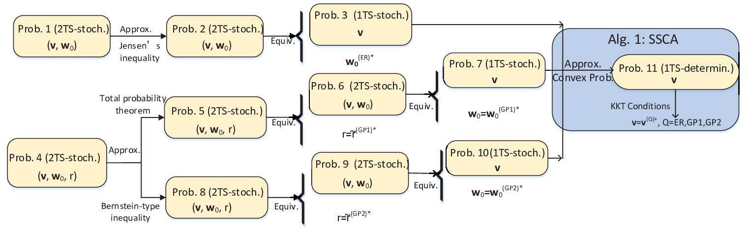
Refer to caption
Fig. 2: Illustration of proposed solution framework. “1TS” and “2TS” are short for “single-timescale” and “two-timescale”, respectively. “stoch.” and “determin.” are short for “stochastic” and “deterministic”, respectively. “Approx”, “Equiv.”, and “Prob.” represent “Approximation”, “Equivalent”, and “Problem”, respectively.

III Maximization of Ergodic Rate

In this section, we consider coding over a large number of slots. First, we formulate a robust optimization problem to maximize the ergodic rate of user 00, which is a challenging two-timescale stochastic non-convex problem. Then, we obtain a closed-form robust instantaneous CSI-adaptive beamforming design for any given phase shifts and a more tractable single-timescale stochastic non-convex approximate problem only for the robust quasi-static phase shifts.

III-A Problem Formulation

We consider coding over a large number of slots. Then, the ergodic rate of user 00, C(E​R)​(𝐯,𝐰0)C^{(ER)}\left(\mathbf{v},\mathbf{w}_{0}\right) (bit/s/Hz), is given by:44 4 For all k∈𝒦\{0}k\in\mathcal{K}\backslash\{0\}, by treating (𝐯H​𝐆k,0+𝐡k,0H)​𝐡k,k‖𝐡k,k‖2​Xk∼C​𝒩​(0,𝔼⁡[|(𝐯H​𝐆k,0+𝐡k,0H)​𝐡k,k‖𝐡k,k‖2|2])\left(\mathbf{v}^{H}\mathbf{G}_{k,0}+\mathbf{h}^{H}_{k,0}\right)\frac{{\mathbf{h}}_{k,k}}{\left\lVert{\mathbf{h}}_{k,k}\right\rVert_{2}}X_{k}\sim C\mathcal{N}\left(0,\mathbb{E}\left[\left\lvert\left(\mathbf{v}^{H}\mathbf{G}_{k,0}+\mathbf{h}^{H}_{k,0}\right)\frac{{\mathbf{h}}_{k,k}}{\left\lVert{\mathbf{h}}_{k,k}\right\rVert_{2}}\right\rvert^{2}\right]\right), which corresponds to the worst-case noise, C(E​R)​(𝐯,𝐰0)C^{(ER)}\left(\mathbf{v},\mathbf{w}_{0}\right) in (7) can be achieved.

C(E​R)​(𝐯,𝐰0)=𝔼⁡[log2⁡(1+P0​|(𝐯H​𝐆0,0+𝐡0,0H)​𝐰0​(𝐇^0)|2∑k∈𝒦\{0}Pk​𝔼​[|(𝐯H​𝐆k,0+𝐡k,0H)​𝐡k,k‖𝐡k,k‖2|2]+σ2)].\displaystyle C^{(ER)}(\mathbf{v},\mathbf{w}_{0})=\mathbb{E}\left[\log_{2}\left(1+\frac{{P_{0}}\left\lvert\left(\mathbf{v}^{H}\mathbf{G}_{0,0}+\mathbf{h}^{H}_{0,0}\right)\mathbf{w}_{0}\left(\hat{\mathbf{H}}_{0}\right)\right\rvert^{2}}{\sum\limits_{k\in\mathcal{K}\backslash\{0\}}{P_{k}}\mathbb{E}\left[{\left\lvert\left(\mathbf{v}^{H}\mathbf{G}_{k,0}+\mathbf{h}^{H}_{k,0}\right)\frac{{\mathbf{h}}_{k,k}}{\left\lVert{\mathbf{h}}_{k,k}\right\rVert_{2}}\right\rvert}^{2}\right]+{\sigma}^{2}}\right)\right]. (7)

We aim to maximize C(E​R)​(𝐯,𝐰0)C^{(ER)}\left(\mathbf{v},\mathbf{w}_{0}\right) by optimizing the phase shifts 𝐯\mathbf{v} and beamforming function 𝐰0\mathbf{w}_{0} subject to the phase shift constraints in (1) and the normalized beamforming constraints in (6).

Problem 1 (Robust Ergodic Rate Maximization)
max𝐯,𝐰0C(E​R)​(𝐯,𝐰0)s.t.(1),(6).\displaystyle\begin{split}\mathop{\max}_{\mathbf{v},\mathbf{w}_{0}}\quad&C^{(ER)}(\mathbf{v},\mathbf{w}_{0})\\ s.t.\quad&\eqref{eq:phi},\quad\eqref{eq:w}.\end{split}
Remark 1 (Robust Design in Problem 1)

An optimal solution of Problem 1 adapts to the variances of the Gaussian estimation errors δ12\delta_{1}^{2} and δ22\delta_{2}^{2} and hence is robust against CSI estimation errors.

Remark 2 (Challenge for Solving Problem 1)

As the objective function does not have an analytical expression, Problem 1 has to be treated as a stochastic optimization problem. As 𝐯\mathbf{v} is constant, 𝐰0​(𝐇^0)\mathbf{w}_{0}(\hat{\mathbf{H}}_{0}) adapts to 𝐇^0\hat{\mathbf{H}}_{0}, and C(E​R)​(𝐯,𝐰0)C^{(ER)}(\mathbf{v},\mathbf{w}_{0}) is non-convex in (𝐯,𝐰0)\left(\mathbf{v},\mathbf{w}_{0}\right), Problem 1 is actually a two-timescale stochastic non-convex optimization problem. Moreover, the number of random variables in Problem 1 is 2​M0​N0​(Mr​Nr+1)2M_{0}N_{0}(M_{r}N_{r}+1), which is usually quite large. Therefore, Problem 1 is very challenging.

Problem Problem 1 Problem 2 Problem 3
Random Variables 𝐇^0,Δ​𝐇0\hat{\mathbf{H}}_{0},\Delta{\mathbf{H}}_{0} 𝐇^0\hat{\mathbf{H}}_{0} 𝐇^0\hat{\mathbf{H}}_{0}
Optimization Variables (𝐯,𝐰0)\left(\mathbf{v},\mathbf{w}_{0}\right) (𝐯,𝐰0)\left(\mathbf{v},\mathbf{w}_{0}\right) 𝐯\mathbf{v}
Constraints (1), (6) (1), (6) (1)
Timescale Two-timescale Two-timescale Single-timescale
TABLE I: Comparisons of the problems in the ergodic rate maximization.

III-B Closed-form Beamforming and Approximate Phase Shift Optimization

First, we simplify the objective function of Problem 1. As in [11, 13], we can obtain an upper bound of C(E​R)​(𝐯,𝐰0)C^{(ER)}(\mathbf{v},\mathbf{w}_{0}) using Jensen’s inequality and channel statistics [37].

Theorem 1 (Upper Bound of C(E​R)​(𝐯,𝐰0)C^{(ER)}(\mathbf{v},\mathbf{w}_{0}))
C(E​R)​(𝐯,𝐰0)≤log2⁡(1+P0​𝔼​[g0(E​R)​(𝐯,𝐰0​(𝐇^0),𝐇^0)]∑k∈𝒦\{0}Pk​gk​(𝐯)+σ2),\displaystyle C^{(ER)}(\mathbf{v},\mathbf{w}_{0})\leq\log_{2}\left(1+\frac{P_{0}\mathbb{E}\left[{g}_{0}^{(ER)}\left(\mathbf{v},\mathbf{w}_{0}\left(\hat{\mathbf{H}}_{0}\right),\hat{\mathbf{H}}_{0}\right)\right]}{\sum\limits_{k\in\mathcal{K}\backslash\{0\}}P_{k}{g}_{k}\left(\mathbf{v}\right)+\sigma^{2}}\right),

where g0(E​R)​(𝐯,𝐰0​(𝐇^0),𝐇^0){g}_{0}^{(ER)}\left(\mathbf{v},\mathbf{w}_{0}\left(\hat{\mathbf{H}}_{0}\right),\hat{\mathbf{H}}_{0}\right) and gk​(𝐯){g}_{k}\left(\mathbf{v}\right) are given by:

g0(E​R)​(𝐯,𝐰0​(𝐇^0),𝐇^0)≜|(𝐯H​𝐆^0,0+𝐡^0,0H)​𝐰0​(𝐇^0)|2+δ22+Mr​Nr​δ12,\displaystyle g_{0}^{(ER)}\left(\mathbf{v},\mathbf{w}_{0}\left(\hat{\mathbf{H}}_{0}\right),\hat{\mathbf{H}}_{0}\right)\triangleq\left\lvert\left(\mathbf{v}^{H}\hat{\mathbf{G}}_{0,0}+\hat{\mathbf{h}}^{H}_{0,0}\right)\mathbf{w}_{0}\left(\hat{\mathbf{H}}_{0}\right)\right\rvert^{2}+\delta_{2}^{2}+M_{r}N_{r}\delta_{1}^{2}, (8)
gk​(𝐯)≜1Mk​Nk​‖𝐯H​𝐆¯k,0‖22+αk,r​αr,0​Mr​Nr​(1−τk)+αk,0,k∈𝒦\{0}.\displaystyle g_{k}\left(\mathbf{v}\right)\triangleq{\color[rgb]{0,0,0}\frac{1}{M_{k}N_{k}}\left\lVert\mathbf{v}^{H}\bar{\mathbf{G}}_{k,0}\right\rVert_{2}^{2}}+\alpha_{k,r}\alpha_{r,0}M_{r}N_{r}\left(1-\tau_{k}\right)+\alpha_{k,0},\quad k\in\mathcal{K}\backslash\{0\}. (9)
Proof:

Please refer to Appendix A. ∎

As the upper bound in Theorem 1 is a good approximation of C(E​R)​(𝐯,𝐰0)C^{(ER)}(\mathbf{v},\mathbf{w}_{0}), which will be seen in Fig. 4, we can consider the maximization of the upper bound instead of Problem 1 [13, 28]. log2⁡(⋅)\log_{2}(\cdot) is an increasing function, so the optimization is equivalent to the following problem, which is simpler than Problem 1, as shown in Table I.

Problem 2 (Approximate Problem of Problem 1)
max𝐯,𝐰0P0​𝔼​[g0(E​R)​(𝐯,𝐰0​(𝐇^0),𝐇^0)]∑k∈𝒦\{0}Pk​gk​(𝐯)+σ2s.t.(1),(6).\begin{split}\mathop{\max}_{\mathbf{v},\mathbf{w}_{0}}\quad&\frac{P_{0}\mathbb{E}\left[{g}_{0}^{(ER)}\left(\mathbf{v},\mathbf{w}_{0}\left(\hat{\mathbf{H}}_{0}\right),\hat{\mathbf{H}}_{0}\right)\right]}{\sum\limits_{k\in\mathcal{K}\backslash\{0\}}P_{k}{g}_{k}\left(\mathbf{v}\right)+\sigma^{2}}\\ s.t.\quad&\eqref{eq:phi},\quad\eqref{eq:w}.\end{split}

Next, using Cauchy-Schwartz inequality and the structural property of Problem 2, we obtain a closed-form robust beamforming design for any given phase shifts and equivalently transform Problem 2, a two-timescale non-convex problem, to a single-timescale stochastic non-convex problem only for the phase shifts, as shown in Table I.

Problem 3 (Equivalent Problem of Problem 2)
max𝐯P0​𝔼𝐇^0​[g0(E​R)​(𝐯,(𝐯H​𝐆^0,0+𝐡^0,0H)H‖𝐯H​𝐆^0,0+𝐡^0,0H‖2,𝐇^0)]∑k∈𝒦\{0}Pk​gk​(𝐯)+σ2s.t.(1).\displaystyle\begin{split}\mathop{\max}_{\mathbf{v}}\quad&\frac{P_{0}\mathbb{E}_{\hat{\mathbf{H}}_{0}}\left[{g}_{0}^{(ER)}\left(\mathbf{v},\frac{\left(\mathbf{v}^{H}\hat{\mathbf{G}}_{0,0}+\hat{\mathbf{h}}^{H}_{0,0}\right)^{H}}{\left\lVert\mathbf{v}^{H}\hat{\mathbf{G}}_{0,0}+\hat{\mathbf{h}}^{H}_{0,0}\right\rVert_{2}},\hat{\mathbf{H}}_{0}\right)\right]}{\sum\limits_{k\in\mathcal{K}\backslash\{0\}}P_{k}{g}_{k}\left(\mathbf{v}\right)+\sigma^{2}}\\ s.t.\quad&\eqref{eq:phi}.\end{split}
Theorem 2 (Equivalence between Problem 2 and Problem 3)

If 𝐯(ER)∗\mathbf{v}^{(ER)*} is an optimal solution of Problem 3, then (𝐯(ER)∗,𝐰0(ER)∗)\left(\mathbf{v}^{(ER)*},\mathbf{w}_{0}^{(ER)*}\right) is an optimal solution of Problem 2, where

𝐰0∗​(𝐇^0)=((𝐯(ER)∗)H𝐆^0,0+𝐡^H0,0)H‖(𝐯(ER)∗)H𝐆^0,0+𝐡^H0,0‖2,𝐇^0∈ℂM0​N0×(Mr​Nr+1).\displaystyle\mathbf{w}_{0}^{*}\left(\hat{\mathbf{H}}_{0}\right)=\frac{\left(\left(\mathbf{v}^{(ER)*}\right)^{H}\hat{\mathbf{G}}_{0,0}+\hat{\mathbf{h}}^{H}_{0,0}\right)^{H}}{\left\lVert\left(\mathbf{v}^{(ER)*}\right)^{H}\hat{\mathbf{G}}_{0,0}+\hat{\mathbf{h}}^{H}_{0,0}\right\rVert_{2}},\quad\hat{\mathbf{H}}_{0}\in\mathbb{C}^{M_{0}N_{0}\times(M_{r}N_{r}+1)}. (10)
Proof:

Please refer to Appendix B. ∎

The closed-form robust instantaneous CSI-adaptive beamforming design (for given 𝐯(ER)∗\mathbf{v}^{(ER)*}) in (10) has computational complexity 𝒪⁡(M0​N0​Mr​Nr)\mathcal{O}(M_{0}N_{0}M_{r}N_{r}) and hence can promptly adapt to rapid CSI changes over slots. In Section V, we will obtain a robust quasi-static phase shift design by solving Problem 3.

IV Maximization of Average Goodput

In this section, we consider coding within each slot and adopt transmission rate adaptation over slots. First, we formulate a robust optimization problem to maximize the average goodput of user 00, which is a more challenging two-timescale stochastic non-convex problem. Then, we obtain two closed-form robust instantaneous CSI-adaptive beamforming and rate adaptation designs for any given phase shifts and two more tractable single-timescale stochastic non-convex approximate problems only for the robust quasi-static phase shifts. Later in Section VI, we will see that the two resulting robust joint designs have average goodput advantages at different system parameters and well complement each other.

IV-A Problem Formulation

We consider coding within one slot. In a slot with imperfect CSIT 𝐇^0\hat{\mathbf{H}}_{0} and actual CSI 𝐇0=𝐇^0+Δ​𝐇0\mathbf{H}_{0}=\hat{\mathbf{H}}_{0}+\Delta{\mathbf{H}}_{0}, the channel capacity of user 00, C⁡(𝐯,𝐰0​(𝐇^0),𝐇^0,Δ​𝐇0)C\left(\mathbf{v},\mathbf{w}_{0}\left(\hat{\mathbf{H}}_{0}\right),\hat{\mathbf{H}}_{0},\Delta{\mathbf{H}}_{0}\right), is given by:

C⁡(𝐯,𝐰0​(𝐇^0),𝐇^0,Δ​𝐇0)=log2⁡(1+P0​|(𝐯H​𝐆0,0+𝐡0,0H)​𝐰0​(𝐇^0)|2∑k∈𝒦\{0}Pk​𝔼​[|(𝐯H​𝐆k,0+𝐡k,0H)​𝐡k,k‖𝐡k,k‖2|2]+σ2).\displaystyle C\left(\mathbf{v},\mathbf{w}_{0}\left(\hat{\mathbf{H}}_{0}\right),\hat{\mathbf{H}}_{0},\Delta{\mathbf{H}}_{0}\right)=\log_{2}\left(1+\frac{{P_{0}}\left\lvert\left(\mathbf{v}^{H}\mathbf{G}_{0,0}+\mathbf{h}^{H}_{0,0}\right)\mathbf{w}_{0}\left(\hat{\mathbf{H}}_{0}\right)\right\rvert^{2}}{\sum\limits_{k\in\mathcal{K}\backslash\{0\}}{P_{k}}\mathbb{E}\left[{\left\lvert\left(\mathbf{v}^{H}\mathbf{G}_{k,0}+\mathbf{h}^{H}_{k,0}\right)\frac{{\mathbf{h}}_{k,k}}{\left\lVert{\mathbf{h}}_{k,k}\right\rVert_{2}}\right\rvert}^{2}\right]+{\sigma}^{2}}\right).

As Δ​𝐇0\Delta\mathbf{H}_{0} is unknown, C⁡(𝐯,𝐰0​(𝐇^0),𝐇^0,Δ​𝐇0)C\left(\mathbf{v},\mathbf{w}_{0}\left(\hat{\mathbf{H}}_{0}\right),\hat{\mathbf{H}}_{0},\Delta{\mathbf{H}}_{0}\right) is unknown to BS 00. Thus, we adopt transmission rate adaptation according to 𝐇^0\hat{\mathbf{H}}_{0}. Let r⁡(𝐇^0)∈ℝr\left(\hat{\mathbf{H}}_{0}\right)\in\mathbb{R} denote the transmission rate of user 00 at 𝐇^0\hat{\mathbf{H}}_{0}. We can view r:ℂM0​N0×(Mr​Nr+1)→ℝr:\mathbb{C}^{M_{0}N_{0}\times(M_{r}N_{r}+1)}\rightarrow\mathbb{R} as a rate adaption function from imperfect CSI to a transmission rate for user 00. The transmission from BS 00 to user 00 is successful if C⁡(𝐯,𝐰0​(𝐇^0),𝐇^0,Δ​𝐇0)≥r⁡(𝐇^0)C\left(\mathbf{v},\mathbf{w}_{0}\left(\hat{\mathbf{H}}_{0}\right),\hat{\mathbf{H}}_{0},\Delta{\mathbf{H}}_{0}\right)\geq r\left(\hat{\mathbf{H}}_{0}\right). We consider the following successful transmission probability constraints:

Pr[C(𝐯,𝐰0(𝐇^0),𝐇^0,Δ𝐇0)≥r(𝐇^0)]≥ρ,𝐇^0∈ℂM0​N0×(Mr​Nr+1),\text{Pr}\left[C\left(\mathbf{v},\mathbf{w}_{0}\left(\hat{\mathbf{H}}_{0}\right),\hat{\mathbf{H}}_{0},\Delta{\mathbf{H}}_{0}\right)\geq r\left(\hat{\mathbf{H}}_{0}\right)\right]\geq\rho,\quad\hat{\mathbf{H}}_{0}\in\mathbb{C}^{M_{0}N_{0}\times(M_{r}N_{r}+1)}, (11)

where ρ∈(0,1)\rho\in(0,1) is the successful transmission probability requirement. The average goodput of user 00 in a slot with 𝐇^0\hat{\mathbf{H}}_{0} is expressed as Pr[C(𝐯,𝐰0(𝐇^0),𝐇^0,Δ𝐇0)≥r(𝐇^0)]r(𝐇^0)\text{Pr}\left[C\left(\mathbf{v},\mathbf{w}_{0}\left(\hat{\mathbf{H}}_{0}\right),\hat{\mathbf{H}}_{0},\Delta{\mathbf{H}}_{0}\right)\geq r\left(\hat{\mathbf{H}}_{0}\right)\right]r\left(\hat{\mathbf{H}}_{0}\right), which is greater than or equal to ρ​r​(𝐇^0)\rho r\left(\hat{\mathbf{H}}_{0}\right) under (11). Then, the average goodput of user 00 over slots, denoted by C(G​P)​(𝐯,𝐰0,r)C^{(GP)}\left(\mathbf{v},\mathbf{w}_{0},r\right), can be defined as:

C(G​P)​(𝐯,𝐰0,r)=ρ​𝔼​[r⁡(𝐇^0)].C^{(GP)}\left(\mathbf{v},\mathbf{w}_{0},r\right)=\rho\mathbb{E}\left[r\left(\hat{\mathbf{H}}_{0}\right)\right]. (12)

We aim to maximize the average goodput of user 00, C(G​P)​(𝐯,𝐰0,r)C^{(GP)}\left(\mathbf{v},\mathbf{w}_{0},r\right), by optimizing the phase shifts 𝐯\mathbf{v}, beamforming function 𝐰0\mathbf{w}_{0}, and rate adaption function rr subject to the phase shift constraints in (1), the normalized beamforming constraints in (6), and the successful transmission probability constraints in (11).

Problem 4 (Robust Average Goodput Maximization)
C(GP)∗≜max𝐯,𝐰0,rC(G​P)​(𝐯,𝐰0,r)s.t.(1),(6),(11).\displaystyle\begin{split}C^{(GP)*}\triangleq\mathop{\max}_{\mathbf{v},\mathbf{w}_{0},r}\quad&C^{(GP)}\left(\mathbf{v},\mathbf{w}_{0},r\right)\\ s.t.\quad&\eqref{eq:phi},\quad\eqref{eq:w},\quad\eqref{eq:proconstraints}.\end{split}
Remark 3 (Robust Design in Problem 4)

An optimal solution of Problem 4 adapts to the variances of the Gaussian estimation errors δ12\delta_{1}^{2} and δ22\delta_{2}^{2} and hence is robust against CSI estimation errors.

Remark 4 (Challenge for Solving Problem 4)

As 𝐯\mathbf{v} is constant, 𝐰0​(𝐇^0)\mathbf{w}_{0}\left(\hat{\mathbf{H}}_{0}\right) and r⁡(𝐇^0)r\left(\hat{\mathbf{H}}_{0}\right) both adapt to 𝐇^0\hat{\mathbf{H}}_{0}, and C(G​P)​(𝐯,𝐰0,r)C^{(GP)}\left(\mathbf{v},\mathbf{w}_{0},r\right) is non-convex in (𝐯,𝐰0,r)\left(\mathbf{v},\mathbf{w}_{0},r\right), Problem 4 is actually a two-timescale stochastic non-convex optimization problem with 2​M0​N0​(Mr​Nr+1)2M_{0}N_{0}(M_{r}N_{r}+1) random variables, which is usually quite large. Besides, Problem 4 has infinitely many successfully transmission constraints, one for each 𝐇^0\hat{\mathbf{H}}_{0}, and an extra function rr to be optimized. Thus, Problem 4 is even more challenging than Problem 1.

Problem Problem 4 Problem 5 Problem 6 Problem 7
Random Variables 𝐇^0,Δ​𝐇0\hat{\mathbf{H}}_{0},\Delta{\mathbf{H}}_{0} 𝐇^0,Δ​𝐇0\hat{\mathbf{H}}_{0},\Delta{\mathbf{H}}_{0} 𝐇^0\hat{\mathbf{H}}_{0} 𝐇^0\hat{\mathbf{H}}_{0}
Optimization Variables (𝐯,𝐰0,r)\left(\mathbf{v},\mathbf{w}_{0},r\right) (𝐯,𝐰0,r)\left(\mathbf{v},\mathbf{w}_{0},r\right) (𝐯,𝐰0)\left(\mathbf{v},\mathbf{w}_{0}\right) 𝐯\mathbf{v}
Constraints (1), (6), (11) (1), (6), (14) (1), (6) (1)
Timescale Two-timescale Two-timescale Two-timescale Single-timescale
TABLE II: Comparisons of the problems in the average goodput maximization based on a deterministic bounded error set.

IV-B Closed-form Beamforming and Approximate Phase Shift Optimization

IV-B1 Approximation based on a deterministic bounded error set

First, we tackle the challenge caused by the infinitely many constraints in (11) via constructing a deterministic bounded set of Δ​𝐇0\Delta\mathbf{H}_{0}:

ℰ≜{(Δ𝐆0,0,Δ𝐡0,0)|‖Δ𝐆0,0‖2≤ε1,‖Δ𝐡0,0‖2≤ε2},\displaystyle\mathcal{E}\triangleq\left\{\left(\Delta{\mathbf{G}}_{0,0},\Delta{\mathbf{h}}_{0,0}\right)\big|\left\lVert\Delta{\mathbf{G}}_{0,0}\right\rVert_{2}\leq\varepsilon_{1},\left\lVert\Delta{\mathbf{h}}_{0,0}\right\rVert_{2}\leq\varepsilon_{2}\right\}, (13)

where ε1\varepsilon_{1} and ε2\varepsilon_{2} are given by:

ε1=δ122​F2​M0​N0​Mr​Nr−1​(ρ),ε2=δ222​F2​M0​N0−1​(ρ).\displaystyle\varepsilon_{1}=\sqrt{\frac{\delta_{1}^{2}}{2}F_{2M_{0}N_{0}M_{r}N_{r}}^{-1}(\rho)},\quad\varepsilon_{2}=\sqrt{\frac{\delta_{2}^{2}}{2}F_{2M_{0}N_{0}}^{-1}(\rho)}.

Here, F2​M0​N0−1​(⋅)F_{2M_{0}N_{0}}^{-1}(\cdot) and F2​M0​N0​Mr​Nr−1​(⋅)F_{2M_{0}N_{0}M_{r}N_{r}}^{-1}(\cdot) denote the inverse cumulative distribution functions (CDFs) of the Chi-square distributions with 2​M0​N02M_{0}N_{0} and 2​M0​N0​Mr​Nr2M_{0}N_{0}M_{r}N_{r} degrees of freedom, respectively. Based on the deterministic bounded error set ℰ\mathcal{E} in (13) and the total probability theorem, we obtain Problem 5, which is an approximate problem of Problem 4.

Problem 5 (Approximate Problem of Problem 4)
C(GP1)∗≜max𝐯,𝐰0,r\displaystyle C^{(GP1)*}\triangleq\mathop{\max}_{\mathbf{v},\mathbf{w}_{0},r}\quad ρ​𝔼​[r⁡(𝐇^0)]\displaystyle\rho\mathbb{E}\left[r\left(\hat{\mathbf{H}}_{0}\right)\right]
s.t.\displaystyle s.t.\quad (1),(6),\displaystyle\eqref{eq:phi},\quad\eqref{eq:w},
Pr​[C⁡(𝐯,𝐰0​(𝐇^0),𝐇^0,Δ​𝐇0)≥r⁡(𝐇^0)|Δ​𝐇0∈ℰ]=1.\displaystyle\text{Pr}\left[C\left(\mathbf{v},\mathbf{w}_{0}\left(\hat{\mathbf{H}}_{0}\right),\hat{\mathbf{H}}_{0},\Delta{\mathbf{H}}_{0}\right)\geq r\left(\hat{\mathbf{H}}_{0}\right)\big|\Delta\mathbf{H}_{0}\in\mathcal{E}\right]=1. (14)

The relationship between Problem 4 and Problem 5 is summarized in the following lemma.

Lemma 1 (Relationship between Problem 4 and Problem 5)

C(GP1)∗≤C(GP)∗C^{(GP1)*}\leq C^{(GP)*}, where C(GP)∗C^{(GP)*} and C(GP1)∗C^{(GP1)*} denote the optimal values of Problem 4 and Problem 5, respectively. Furthermore, a feasible solution of Problem 5 is feasible for Problem 4.

Proof:

Please refer to Appendix C. ∎

Define:

g0(G​P​1)​(𝐯,𝐰0​(𝐇^0),𝐇^0)≜(|(𝐯H​𝐆^0,0+𝐡^0,0H)​𝐰0​(𝐇^0)|−ε1​Mr​Nr−ε2)2.\displaystyle g_{0}^{(GP1)}\left(\mathbf{v},\mathbf{w}_{0}\left(\hat{\mathbf{H}}_{0}\right),\hat{\mathbf{H}}_{0}\right)\triangleq\left(\left\lvert\left(\mathbf{v}^{H}\hat{\mathbf{G}}_{0,0}+\hat{\mathbf{h}}_{0,0}^{H}\right)\mathbf{w}_{0}\left(\hat{\mathbf{H}}_{0}\right)\right\rvert-\varepsilon_{1}\sqrt{M_{r}N_{r}}-\varepsilon_{2}\right)^{2}. (15)

Using Cauchy-Schwartz inequality and the structural property of Problem 5, we equivalently convert Problem 5 to the following problem.

Problem 6 (Equivalent Problem of Problem 5)
max𝐯ρ𝔼[r~(GP1)∗(𝐯,𝐇^0)]s.t.(1),\displaystyle\begin{split}\mathop{\max}_{\mathbf{v}}\quad&\rho\mathbb{E}\left[\tilde{r}^{(GP1)*}\left(\mathbf{v},\hat{\mathbf{H}}_{0}\right)\right]\\ s.t.\quad&\eqref{eq:phi},\end{split} (16)

where

r~(GP1)∗(𝐯,𝐇^0)=max𝐰0log2⁡(1+g0(G​P​1)​(𝐯,𝐰0​(𝐇^0),𝐇^0)∑k∈𝒦\{0}Pk​gk​(𝐯)+σ2)s.t.(6).\displaystyle\begin{split}\tilde{r}^{(GP1)*}\left(\mathbf{v},\hat{\mathbf{H}}_{0}\right)=\mathop{\max}\limits_{\mathbf{w}_{0}}\quad&\log_{2}\left(1+\frac{g_{0}^{(GP1)}\left(\mathbf{v},\mathbf{w}_{0}\left(\hat{\mathbf{H}}_{0}\right),\hat{\mathbf{H}}_{0}\right)}{\sum\limits_{k\in\mathcal{K}\backslash\{0\}}P_{k}{g}_{k}\left(\mathbf{v}\right)+\sigma^{2}}\right)\\ s.t.\quad&\eqref{eq:w}.\end{split} (17)

Let 𝐯~(GP1)∗\tilde{\mathbf{v}}^{(GP1)*} and 𝐰~0(GP1)∗(𝐯,𝐇^0)\tilde{\mathbf{w}}_{0}^{(GP1)*}\left(\mathbf{v},\hat{\mathbf{H}}_{0}\right) denote the optimal solutions of the problems in (16) and (17), respectively.

Lemma 2 (Equivalence between Problem 5 and Problem 6 )

The optimal solution and optimal value of the problem in (17) are given by:

𝐰~0(GP1)∗(𝐯,𝐇^0)=\displaystyle\tilde{\mathbf{w}}_{0}^{(GP1)*}\left(\mathbf{v},\hat{\mathbf{H}}_{0}\right)= (𝐯H​𝐆^0,0+𝐡^0,0H)H‖𝐯H​𝐆^0,0+𝐡^0,0H‖2,\displaystyle\frac{\left(\mathbf{v}^{H}\hat{\mathbf{G}}_{0,0}+\hat{\mathbf{h}}^{H}_{0,0}\right)^{H}}{\left\lVert\mathbf{v}^{H}\hat{\mathbf{G}}_{0,0}+\hat{\mathbf{h}}^{H}_{0,0}\right\rVert_{2}}, (18)
r~(GP1)∗(𝐯,𝐇^0)=\displaystyle\tilde{r}^{(GP1)*}\left(\mathbf{v},\hat{\mathbf{H}}_{0}\right)= log2⁡(1+g0(G​P​1)(𝐯,𝐰~0(GP1)∗(𝐯,𝐇^0),𝐇^0)∑k∈𝒦\{0}Pk​gk​(𝐯)+σ2),\displaystyle\log_{2}\left(1+\frac{g_{0}^{(GP1)}\left(\mathbf{v},\tilde{\mathbf{w}}_{0}^{(GP1)*}\left(\mathbf{v},\hat{\mathbf{H}}_{0}\right),\hat{\mathbf{H}}_{0}\right)}{\sum\limits_{k\in\mathcal{K}\backslash\{0\}}P_{k}{g}_{k}\left(\mathbf{v}\right)+\sigma^{2}}\right), (19)

where g0(G​P​1)​(⋅)g_{0}^{(GP1)}\left(\cdot\right) is given by (15). Furthermore, (𝐯~(GP1)∗,𝐰~0(GP1)∗(𝐯~(GP1)∗,𝐇^0),r~(GP1)∗(𝐯~(GP1)∗,𝐇^0))\left(\tilde{\mathbf{v}}^{(GP1)*},\tilde{\mathbf{w}}_{0}^{(GP1)*}\left(\tilde{\mathbf{v}}^{(GP1)*},\hat{\mathbf{H}}_{0}\right),\tilde{r}^{(GP1)*}\left(\tilde{\mathbf{v}}^{(GP1)*},\hat{\mathbf{H}}_{0}\right)\right) is an optimal solution of Problem 5.

Proof:

Please refer to Appendix D. ∎

By Lemma 2, we equivalently transform Problem 6 to a single-timescale stochastic non-convex problem only for the phase shifts, as shown in Table II.

Problem 7 (Equivalent Problem of Problem 6)
max𝐯P0​𝔼​[g0(G​P​1)​(𝐯,(𝐯H​𝐆^0,0+𝐡^0,0H)H‖𝐯H​𝐆^0,0+𝐡^0,0H‖2,𝐇^0)]∑k∈𝒦\{0}Pk​gk​(𝐯)+σ2s.t.(1).\displaystyle\begin{split}\mathop{\max}_{\mathbf{v}}\quad&\frac{P_{0}\mathbb{E}\left[{g}_{0}^{(GP1)}\left(\mathbf{v},\frac{\left(\mathbf{v}^{H}\hat{\mathbf{G}}_{0,0}+\hat{\mathbf{h}}^{H}_{0,0}\right)^{H}}{\left\lVert\mathbf{v}^{H}\hat{\mathbf{G}}_{0,0}+\hat{\mathbf{h}}^{H}_{0,0}\right\rVert_{2}},\hat{\mathbf{H}}_{0}\right)\right]}{\sum\limits_{k\in\mathcal{K}\backslash\{0\}}P_{k}{g}_{k}\left(\mathbf{v}\right)+\sigma^{2}}\\ s.t.\quad&\eqref{eq:phi}.\end{split}
Theorem 3 (Equivalence between Problem 5 and Problem 7)

If 𝐯~(GP1)∗\tilde{\mathbf{v}}^{(GP1)*} is an optimal solution of Problem 7, then (𝐯(GP1)∗,𝐰0(GP1)∗,r(GP1)∗)\left(\mathbf{v}^{(GP1)*},\mathbf{w}_{0}^{(GP1)*},r^{(GP1)*}\right) is an optimal solution of Problem 5, where 𝐯(GP1)∗=𝐯~(GP1)∗\mathbf{v}^{(GP1)*}=\tilde{\mathbf{v}}^{(GP1)*} and

𝐰0(GP1)∗(𝐇^0)=\displaystyle\mathbf{w}_{0}^{(GP1)*}\left(\hat{\mathbf{H}}_{0}\right)= 𝐰~0(GP1)∗(𝐯~(GP1)∗,𝐇^0),\displaystyle\tilde{\mathbf{w}}^{(GP1)*}_{0}\left(\tilde{\mathbf{v}}^{(GP1)*},\hat{\mathbf{H}}_{0}\right), (20)
r(GP1)∗(𝐇^0)=\displaystyle r^{(GP1)*}\left(\hat{\mathbf{H}}_{0}\right)= r~(GP1)∗(𝐯~(GP1)∗,𝐇^0),𝐇^0∈ℂM0​N0×(Mr​Nr+1),\displaystyle\tilde{r}^{(GP1)*}\left(\tilde{\mathbf{v}}^{(GP1)*},\hat{\mathbf{H}}_{0}\right),\quad\hat{\mathbf{H}}_{0}\in\mathbb{C}^{M_{0}N_{0}\times(M_{r}N_{r}+1)}, (21)

where 𝐰0(GP1)∗(⋅)\mathbf{w}_{0}^{(GP1)*}(\cdot) and r(GP1)∗(⋅)r^{(GP1)*}(\cdot) are given by (18) and (19), respectively.

Proof:

Please refer to Appendix E. ∎

Similarly, the closed-form robust instantaneous CSI-adaptive beamforming and rate adaptation design for given 𝐯(GP1)∗\mathbf{v}^{(GP1)*} in (20) and (21) has computational complexity 𝒪⁡(M0​N0​Mr​Nr)\mathcal{O}(M_{0}N_{0}M_{r}N_{r}) and hence can promptly adapt to rapid CSI changes over slots. In Section V, we will obtain a robust quasi-static phase shift design by solving Problem 7.

Problem Problem 4 Problem 8 Problem 9 Problem 10
Random Variables 𝐇^0,Δ​𝐇0\hat{\mathbf{H}}_{0},\Delta{\mathbf{H}}_{0} 𝐇^0,Δ​𝐇0\hat{\mathbf{H}}_{0},\Delta{\mathbf{H}}_{0} 𝐇^0\hat{\mathbf{H}}_{0} 𝐇^0\hat{\mathbf{H}}_{0}
Optimization Variables (𝐯,𝐰0,r)\left(\mathbf{v},\mathbf{w}_{0},r\right) (𝐯,𝐰0,r)\left(\mathbf{v},\mathbf{w}_{0},r\right) (𝐯,𝐰0)\left(\mathbf{v},\mathbf{w}_{0}\right) 𝐯\mathbf{v}
Constraints (1), (6), (11) (1), (6), (22) (1), (6) (1)
Timescale Two-timescale Two-timescale Two-timescale Single-timescale
TABLE III: Comparisons of the problems in the average goodput maximization based on the Bernstein-type inequality.

IV-B2 Approximation based on the Bernstein-type inequality

First, we address the challenge caused by the infinitely many constraints in (11) using the Bernstein-type inequality. Based on the Bernstein-type inequality [38] and the structural property of Problem 4, (11) can be approximated to (please refer to Appendix F for details):

δ12​Mr​Nr+δ22+|(𝐡^0,0H+𝐯H​𝐆^0,0)​𝐰0​(𝐇^0)|2−1P0​(2r⁡(𝐇^0)−1)​(∑k∈𝒦\{0}Pk​gk​(𝐯)+σ2)\displaystyle\delta_{1}^{2}M_{r}N_{r}+\delta_{2}^{2}+\left\lvert\left(\hat{\mathbf{h}}_{0,0}^{H}+\mathbf{v}^{H}\hat{\mathbf{G}}_{0,0}\right)\mathbf{w}_{0}\left(\hat{\mathbf{H}}_{0}\right)\right\rvert^{2}-\frac{1}{P_{0}}\left(2^{r\left(\hat{\mathbf{H}}_{0}\right)}-1\right)\left(\sum\limits_{k\in\mathcal{K}\backslash\{0\}}P_{k}g_{k}(\mathbf{v})+\sigma^{2}\right)
−2​ln⁡11−ρ​((δ12​Mr​Nr+δ22)2+2​(δ12​Mr​Nr+δ22)​|(𝐡^0,0H+𝐯H​𝐆^0,0)​𝐰0​(𝐇^0)|2)≥0.\displaystyle-\sqrt{2\ln\frac{1}{1-\rho}\left(\left(\delta_{1}^{2}M_{r}N_{r}+\delta_{2}^{2}\right)^{2}+2\left(\delta_{1}^{2}M_{r}N_{r}+\delta_{2}^{2}\right)\left\lvert\left(\hat{\mathbf{h}}_{0,0}^{H}+\mathbf{v}^{H}\hat{\mathbf{G}}_{0,0}\right)\mathbf{w}_{0}\left(\hat{\mathbf{H}}_{0}\right)\right\rvert^{2}\right)}\geq 0. (22)

Thus, Problem 4 can be approximated to the following problem.

Problem 8 (Approximate Problem of Problem 4)
max𝐯,𝐰0,r\displaystyle\mathop{\max}_{\mathbf{v},\mathbf{w}_{0},r}\quad ρ​𝔼​[r⁡(𝐇^0)]\displaystyle\rho\mathbb{E}\left[r\left(\hat{\mathbf{H}}_{0}\right)\right]
s.t.\displaystyle s.t.\quad (1),(6),(22).\displaystyle\eqref{eq:phi},\quad\eqref{eq:w},\quad\eqref{eq:constraint1}.

The relationship between Problem 4 and Problem 8 is summarized in the following lemma.

Lemma 3 (Relationship between Problem 4 and Problem 8)

If a feasible solution of Problem 8, (𝐯(G​P​2),𝐰0(G​P​2),r(G​P​2))\left(\mathbf{v}^{(GP2)},\mathbf{w}_{0}^{(GP2)},r^{(GP2)}\right), satisfies (11), then (𝐯(G​P​2),𝐰0(G​P​2),r(G​P​2))\left(\mathbf{v}^{(GP2)},\mathbf{w}_{0}^{(GP2)},r^{(GP2)}\right) is a feasible solution of Problem 4; otherwise, (𝐯(G​P​2),𝐰0(G​P​2),r^(G​P​2))\left(\mathbf{v}^{(GP2)},\mathbf{w}_{0}^{(GP2)},\hat{r}^{(GP2)}\right) is feasible for Problem 4, where r^(G​P​2)\hat{r}^{(GP2)} is given by:

r^(G​P​2)​(𝐇^0)=\displaystyle\hat{r}^{(GP2)}\left(\hat{\mathbf{H}}_{0}\right)= log2⁡(1+g0(G​P​1)​(𝐯(G​P​2),𝐰0(G​P​2)​(𝐇^0),𝐇^0)∑k∈𝒦\{0}Pk​gk​(𝐯(G​P​2))+σ2).\displaystyle\log_{2}\left(1+\frac{g_{0}^{(GP1)}\left(\mathbf{v}^{(GP2)},\mathbf{w}_{0}^{(GP2)}\left(\hat{\mathbf{H}}_{0}\right),\hat{\mathbf{H}}_{0}\right)}{\sum\limits_{k\in\mathcal{K}\backslash\{0\}}P_{k}{g}_{k}\left(\mathbf{v}^{(GP2)}\right)+\sigma^{2}}\right). (23)
Proof:

Please refer to Appendix G. ∎

Define:

g0(G​P​2)​(𝐯,𝐰0​(𝐇^0),𝐇^0)=|(𝐡^0,0H+𝐯H​𝐆^0,0)​𝐰0​(𝐇^0)|2+δ12​Mr​Nr+δ22\displaystyle g_{0}^{(GP2)}\left(\mathbf{v},\mathbf{w}_{0}\left(\hat{\mathbf{H}}_{0}\right),\hat{\mathbf{H}}_{0}\right)=\left\lvert\left(\hat{\mathbf{h}}_{0,0}^{H}+\mathbf{v}^{H}\hat{\mathbf{G}}_{0,0}\right)\mathbf{w}_{0}\left(\hat{\mathbf{H}}_{0}\right)\right\rvert^{2}+\delta_{1}^{2}M_{r}N_{r}+\delta_{2}^{2}
−\displaystyle- 2​ln⁡11−ρ​((δ12​Mr​Nr+δ22)2+2​(δ12​Mr​Nr+δ22)​|(𝐡^0,0H+𝐯H​𝐆^0,0)​𝐰0​(𝐇^0)|2).\displaystyle\sqrt{2\ln\frac{1}{1-\rho}\left(\left(\delta_{1}^{2}M_{r}N_{r}+\delta_{2}^{2}\right)^{2}+2\left(\delta_{1}^{2}M_{r}N_{r}+\delta_{2}^{2}\right)\left\lvert\left(\hat{\mathbf{h}}_{0,0}^{H}+\mathbf{v}^{H}\hat{\mathbf{G}}_{0,0}\right)\mathbf{w}_{0}\left(\hat{\mathbf{H}}_{0}\right)\right\rvert^{2}\right)}. (24)

Using Cauchy-Schwartz inequality and the structural property of Problem 8, we equivalently convert Problem 8 to the following problem.

Problem 9 (Equivalent Problem of Problem 8)
max𝐯ρ𝔼[r~(GP2)∗(𝐯,𝐇^0)]s.t.(1),\displaystyle\begin{split}\mathop{\max}_{\mathbf{v}}\quad&\rho\mathbb{E}\left[\tilde{r}^{(GP2)*}\left(\mathbf{v},\hat{\mathbf{H}}_{0}\right)\right]\\ s.t.\quad&\eqref{eq:phi},\end{split} (25)

where

r~(GP2)∗(𝐯,𝐇^0)=max𝐰0log2⁡(1+g0(G​P​2)​(𝐯,𝐰0​(𝐇^0),𝐇^0)∑k∈𝒦\{0}Pk​gk​(𝐯)+σ2)s.t.(6).\displaystyle\begin{split}\tilde{r}^{(GP2)*}\left(\mathbf{v},\hat{\mathbf{H}}_{0}\right)=\mathop{\max}\limits_{\mathbf{w}_{0}}\quad&\log_{2}\left(1+\frac{g_{0}^{(GP2)}\left(\mathbf{v},\mathbf{w}_{0}\left(\hat{\mathbf{H}}_{0}\right),\hat{\mathbf{H}}_{0}\right)}{\sum\limits_{k\in\mathcal{K}\backslash\{0\}}P_{k}{g}_{k}\left(\mathbf{v}\right)+\sigma^{2}}\right)\\ s.t.\quad&\eqref{eq:w}.\end{split} (26)

Let 𝐯~(GP2)∗\tilde{\mathbf{v}}^{(GP2)*} and 𝐰~0(GP2)∗(𝐯,𝐇^0)\tilde{\mathbf{w}}_{0}^{(GP2)*}\left(\mathbf{v},\hat{\mathbf{H}}_{0}\right) denote the optimal solutions of the problems in (25) and (26), respectively.

Lemma 4 (Equivalence between Problem 8 and Problem 9 )

The optimal solution and optimal value of the problem in (26) are given by:

𝐰~0(GP2)∗(𝐯,𝐇^0)=\displaystyle\tilde{\mathbf{w}}_{0}^{(GP2)*}\left(\mathbf{v},\hat{\mathbf{H}}_{0}\right)= (𝐯H​𝐆^0,0+𝐡^0,0H)H‖𝐯H​𝐆^0,0+𝐡^0,0H‖2,\displaystyle\frac{\left(\mathbf{v}^{H}\hat{\mathbf{G}}_{0,0}+\hat{\mathbf{h}}^{H}_{0,0}\right)^{H}}{\left\lVert\mathbf{v}^{H}\hat{\mathbf{G}}_{0,0}+\hat{\mathbf{h}}^{H}_{0,0}\right\rVert_{2}}, (27)
r~(GP2)∗(𝐯,𝐇^0)=\displaystyle\tilde{r}^{(GP2)*}\left(\mathbf{v},\hat{\mathbf{H}}_{0}\right)= log2⁡(1+g0(G​P​2)(𝐯,𝐰~0(GP2)∗(𝐯,𝐇^0),𝐇^0)∑k∈𝒦\{0}Pk​gk​(𝐯)+σ2),\displaystyle\log_{2}\left(1+\frac{g_{0}^{(GP2)}\left(\mathbf{v},\tilde{\mathbf{w}}_{0}^{(GP2)*}\left(\mathbf{v},\hat{\mathbf{H}}_{0}\right),\hat{\mathbf{H}}_{0}\right)}{\sum\limits_{k\in\mathcal{K}\backslash\{0\}}P_{k}{g}_{k}\left(\mathbf{v}\right)+\sigma^{2}}\right), (28)

where g0(G​P​2)​(⋅)g_{0}^{(GP2)}\left(\cdot\right) is given by (24). Furthermore, (𝐯~(GP2)∗,𝐰~0(GP2)∗(𝐯~(GP2)∗,𝐇^0),r~(GP2)∗(𝐯~(GP2)∗,𝐇^0))\left(\tilde{\mathbf{v}}^{(GP2)*},\tilde{\mathbf{w}}_{0}^{(GP2)*}\left(\tilde{\mathbf{v}}^{(GP2)*},\hat{\mathbf{H}}_{0}\right),\tilde{r}^{(GP2)*}\left(\tilde{\mathbf{v}}^{(GP2)*},\hat{\mathbf{H}}_{0}\right)\right) is an optimal solution of Problem 8.

Proof:

Please refer to Appendix H. ∎

By Lemma 4, we equivalently transform Problem 9 to a more tractable single-timescale stochastic non-convex problem as shown in Table III.

Problem 10 (Equivalent Problem of Problem 9)
max𝐯P0​𝔼​[g0(G​P​2)​(𝐯,(𝐯H​𝐆^0,0+𝐡^0,0H)H‖𝐯H​𝐆^0,0+𝐡^0,0H‖2,𝐇^0)]∑k∈𝒦\{0}Pk​gk​(𝐯)+σ2s.t.(1).\displaystyle\begin{split}\mathop{\max}_{\mathbf{v}}\quad&\frac{P_{0}\mathbb{E}\left[{g}_{0}^{(GP2)}\left(\mathbf{v},\frac{\left(\mathbf{v}^{H}\hat{\mathbf{G}}_{0,0}+\hat{\mathbf{h}}^{H}_{0,0}\right)^{H}}{\left\lVert\mathbf{v}^{H}\hat{\mathbf{G}}_{0,0}+\hat{\mathbf{h}}^{H}_{0,0}\right\rVert_{2}},\hat{\mathbf{H}}_{0}\right)\right]}{\sum\limits_{k\in\mathcal{K}\backslash\{0\}}P_{k}{g}_{k}\left(\mathbf{v}\right)+\sigma^{2}}\\ s.t.\quad&\eqref{eq:phi}.\end{split}
Theorem 4 (Equivalence between Problem 8 and Problem 10)

If 𝐯~(GP2)∗\tilde{\mathbf{v}}^{(GP2)*} is an optimal solution of Problem 10, then (𝐯(GP2)∗,𝐰0(GP2)∗,r(GP2)∗)\left(\mathbf{v}^{(GP2)*},\mathbf{w}_{0}^{(GP2)*},r^{(GP2)*}\right) is an optimal solution of Problem 8, where 𝐯(GP2)∗=𝐯~(GP2)∗\mathbf{v}^{(GP2)*}=\tilde{\mathbf{v}}^{(GP2)*} and

𝐰0(GP2)∗(𝐇^0)=\displaystyle\mathbf{w}_{0}^{(GP2)*}\left(\hat{\mathbf{H}}_{0}\right)= 𝐰~0(GP2)∗(𝐯~(GP2)∗,𝐇^0),\displaystyle\tilde{\mathbf{w}}^{(GP2)*}_{0}\left(\tilde{\mathbf{v}}^{(GP2)*},\hat{\mathbf{H}}_{0}\right), (29)
r(GP2)∗(𝐇^0)=\displaystyle r^{(GP2)*}\left(\hat{\mathbf{H}}_{0}\right)= r~(GP2)∗(𝐯~(GP2)∗,𝐇^0),𝐇^0∈ℂM0​N0×(Mr​Nr+1),\displaystyle\tilde{r}^{(GP2)*}\left(\tilde{\mathbf{v}}^{(GP2)*},\hat{\mathbf{H}}_{0}\right),\quad\hat{\mathbf{H}}_{0}\in\mathbb{C}^{M_{0}N_{0}\times(M_{r}N_{r}+1)}, (30)

where 𝐰0(GP2)∗(⋅)\mathbf{w}_{0}^{(GP2)*}\left(\cdot\right) and r(GP2)∗(⋅)r^{(GP2)*}\left(\cdot\right) are given by (27) and (28), respectively.

Proof:

Please refer to Appendix I. ∎

Analogously, the closed-form robust instantaneous CSI-adaptive beamforming and rate adaptation design (for given 𝐯(GP2)∗\mathbf{v}^{(GP2)*}) in (29) and (30) has computational complexity 𝒪⁡(M0​N0​Mr​Nr)\mathcal{O}(M_{0}N_{0}M_{r}N_{r}) and hence can promptly adapt to rapid CSI changes over slots. In Section V, we will obtain a robust quasi-static phase shift design by solving Problem 10.

V Algorithm for Phase Shift Optimization

Recall that we have obtained closed-form robust instantaneous CSI-adaptive beamforming designs in Section III-B and Section IV-B. It remains to obtain robust quasi-static phase shift designs by solving Problem 3, Problem 7, and Problem 10. Problem 3, Problem 7, and Problem 10 are stochastic non-convex optimization problems with similar non-convex objective functions and the same non-convex constraint functions. This section proposes a low-complexity algorithm to obtain KKT points of each of the three stochastic non-convex problems using SSCA [39].

Specifically, at each iteration tt, we randomly generate LL channel samples, denoted by 𝐇^0,l(t),l=1,…,L\hat{\mathbf{H}}_{0,l}^{(t)},l=1,...,L, according to the distribution of 𝐇^0\hat{\mathbf{H}}_{0} given in Section II. Based on the samples, we approximate each of the three objective functions in Problem 3, Problem 7, and Problem 10 around 𝐯(t−1)\mathbf{v}^{(t-1)} with a concave surrogate function, where 𝐯(t−1)≜(vn(t−1))n∈𝒩\mathbf{v}^{(t-1)}\triangleq\left(v^{(t-1)}_{n}\right)_{n\in\mathcal{N}} denotes the phase shifts at iteration t−1t-1. The surrogate functions for Problem 3, Problem 7, and Problem 10, denoted by f(E​R,t)​(𝐯)f^{(ER,t)}(\mathbf{v}), f(G​P​1,t)​(𝐯)f^{(GP1,t)}(\mathbf{v}), and f(G​P​2,t)​(𝐯)f^{(GP2,t)}(\mathbf{v}), respectively, are given by:

f(Q,t)​(𝐯)=c0(Q,t)+2​R​e​{∑n∈𝒩c1,n(Q,t)​(vn−vn(Q,t−1))}−τ​∑n∈𝒩|vn−vn(Q,t−1)|2,\displaystyle f^{(Q,t)}(\mathbf{v})=c_{0}^{(Q,t)}+2Re\left\{\sum\limits_{n\in\mathcal{N}}c_{1,n}^{(Q,t)}\left(v_{n}-v_{n}^{(Q,t-1)}\right)\right\}-\tau\sum\limits_{n\in\mathcal{N}}\left\lvert v_{n}-v^{(Q,t-1)}_{n}\right\rvert^{2},
Q=E​R,G​P​1,G​P​2,\displaystyle Q=ER,GP1,GP2, (31)

where c0(Q,t)∈ℂc_{0}^{(Q,t)}\in\mathbb{C} and c1,n(Q,t)∈ℂ,n∈𝒩c_{1,n}^{(Q,t)}\in\mathbb{C},n\in\mathcal{N} are updated according to:

c0(Q,t)=\displaystyle c_{0}^{(Q,t)}= ρ(t)​∑l=1Lγ(Q)​(𝐯(Q,t−1),𝐰0,l(t)​(𝐇^0),𝐇^l(t))L+(1−ρ(t))​c0(Q,t−1),\displaystyle\rho^{(t)}\sum\limits_{l=1}^{L}\frac{\gamma^{(Q)}\left(\mathbf{v}^{(Q,t-1)},\mathbf{w}_{0,l}^{(t)}\left(\hat{\mathbf{H}}_{0}\right),\hat{\mathbf{H}}_{l}^{(t)}\right)}{L}+\left(1-\rho^{(t)}\right)c_{0}^{(Q,t-1)}, (32)
c1,n(Q,t)=\displaystyle c^{(Q,t)}_{1,n}= ρ(t)​∑l=1L∂∂vn​γ(Q)​(𝐯(Q,t−1),𝐰0,l(t)​(𝐇^0),𝐇^l(t))L+(1−ρ(t))​c1,n(Q,t),n∈𝒩,\displaystyle\rho^{(t)}\sum\limits_{l=1}^{L}\frac{\frac{\partial}{\partial v_{n}}\gamma^{(Q)}\left(\mathbf{v}^{(Q,t-1)},\mathbf{w}_{0,l}^{(t)}\left(\hat{\mathbf{H}}_{0}\right),\hat{\mathbf{H}}_{l}^{(t)}\right)}{L}+\left(1-\rho^{(t)}\right)c^{(Q,t)}_{1,n},\quad n\in\mathcal{N}, (33)

with c0(Q,0)=0c_{0}^{(Q,0)}=0 and c1,n(Q,0)=0,n∈𝒩c^{(Q,0)}_{1,n}=0,n\in\mathcal{N}. Here, τ>0\tau>0 can be any constant, the term τ​∑n=1Mr​Nr|vn−vn(Q,t−1)|2\tau\sum\limits_{n=1}^{M_{r}N_{r}}\left\lvert v_{n}-v^{(Q,t-1)}_{n}\right\rvert^{2} is used to ensure strong concavity, ρ(t)\rho^{(t)} is a positive diminishing stepsize satisfying:

ρ(t)>0,limt→∞ρ(t)=0,∑t=1∞ρ(t)=∞,∑t=1∞(ρ(t))2<∞,\displaystyle\rho^{(t)}>0,\quad\lim_{t\to\infty}\rho^{(t)}=0,\quad\sum_{t=1}^{\infty}\rho^{(t)}=\infty,\quad\sum_{t=1}^{\infty}\left(\rho^{(t)}\right)^{2}<\infty,

and γ(Q)​(𝐯(Q,t−1),𝐰0,l(t)​(𝐇^0),𝐇^l(t))\gamma^{(Q)}\left(\mathbf{v}^{(Q,t-1)},\mathbf{w}_{0,l}^{(t)}\left(\hat{\mathbf{H}}_{0}\right),\hat{\mathbf{H}}_{l}^{(t)}\right) is given by:

γ(Q)​(𝐯(Q,t−1),𝐰0,l(t)​(𝐇^0),𝐇^l(t))≜{P0​g0(E​R)​(𝐯,(𝐯H​𝐆^0,0+𝐡^0,0H)H‖𝐯H​𝐆^0,0+𝐡^0,0H‖2,𝐇^0)∑k∈𝒦\{0}Pk​gk​(𝐯)+σ2,Q=E​R,P0​g0(G​P​1)​(𝐯,(𝐯H​𝐆^0,0+𝐡^0,0H)H‖𝐯H​𝐆^0,0+𝐡^0,0H‖2,𝐇^0)∑k∈𝒦\{0}Pk​gk​(𝐯)+σ2,Q=G​P​1,P0​g0(G​P​2)​(𝐯,(𝐯H​𝐆^0,0+𝐡^0,0H)H‖𝐯H​𝐆^0,0+𝐡^0,0H‖2,𝐇^0)∑k∈𝒦\{0}Pk​gk​(𝐯)+σ2,Q=G​P​2.\displaystyle\gamma^{(Q)}\left(\mathbf{v}^{(Q,t-1)},\mathbf{w}_{0,l}^{(t)}\left(\hat{\mathbf{H}}_{0}\right),\hat{\mathbf{H}}_{l}^{(t)}\right)\triangleq\begin{cases}\frac{P_{0}{g}_{0}^{(ER)}\left(\mathbf{v},\frac{\left(\mathbf{v}^{H}\hat{\mathbf{G}}_{0,0}+\hat{\mathbf{h}}^{H}_{0,0}\right)^{H}}{\left\lVert\mathbf{v}^{H}\hat{\mathbf{G}}_{0,0}+\hat{\mathbf{h}}^{H}_{0,0}\right\rVert_{2}},\hat{\mathbf{H}}_{0}\right)}{\sum\limits_{k\in\mathcal{K}\backslash\{0\}}P_{k}{g}_{k}\left(\mathbf{v}\right)+\sigma^{2}},\quad&Q=ER,\\ \frac{P_{0}{g}_{0}^{(GP1)}\left(\mathbf{v},\frac{\left(\mathbf{v}^{H}\hat{\mathbf{G}}_{0,0}+\hat{\mathbf{h}}^{H}_{0,0}\right)^{H}}{\left\lVert\mathbf{v}^{H}\hat{\mathbf{G}}_{0,0}+\hat{\mathbf{h}}^{H}_{0,0}\right\rVert_{2}},\hat{\mathbf{H}}_{0}\right)}{\sum\limits_{k\in\mathcal{K}\backslash\{0\}}P_{k}{g}_{k}\left(\mathbf{v}\right)+\sigma^{2}},\quad&Q=GP1,\\ \frac{P_{0}{g}_{0}^{(GP2)}\left(\mathbf{v},\frac{\left(\mathbf{v}^{H}\hat{\mathbf{G}}_{0,0}+\hat{\mathbf{h}}^{H}_{0,0}\right)^{H}}{\left\lVert\mathbf{v}^{H}\hat{\mathbf{G}}_{0,0}+\hat{\mathbf{h}}^{H}_{0,0}\right\rVert_{2}},\hat{\mathbf{H}}_{0}\right)}{\sum\limits_{k\in\mathcal{K}\backslash\{0\}}P_{k}{g}_{k}\left(\mathbf{v}\right)+\sigma^{2}},\quad&Q=GP2.\end{cases}

Furthermore, the non-convex constraints in (1) can be equivalently converted to the convex constraints:

|vn|≤1,n∈𝒩,\displaystyle\lvert v_{n}\rvert\leq 1,\quad n\in\mathcal{N}, (34)

without affecting the optimality [10]. Then, the resulting approximate convex problems at iteration tt are given as follows.

Problem 11 (Approximation of Problem 3, Problem 7, and Problem 10 at Iteration tt)

For Q=E​R,G​P​1,G​P​2Q=ER,GP1,GP2,

𝐯¯(Q,t)=argmax𝐯\displaystyle\bar{\mathbf{v}}^{(Q,t)}=\mathop{\arg}\mathop{\max}_{\mathbf{v}}\quad f(Q,t)​(𝐯),\displaystyle f^{(Q,t)}(\mathbf{v}),
s.t.\displaystyle s.t.\quad (34),\displaystyle\eqref{eq:cvxphi},

where f(Q,t)​(𝐯)f^{(Q,t)}(\mathbf{v}) is given by (31).

As Slater’s condition is satisfied, strong duality holds for Problem 11. Thus, based on problem decomposition and the KKT conditions, we can obtain a closed-form optimal solution of Problem 11.

Theorem 5 (Optimal Solution of Problem 11)

For Q=E​R,G​P​1,G​P​2Q=ER,GP1,GP2, the optimal solution of Problem 11 is given by 𝐯¯(Q,t)=(v¯n(Q,t))n∈𝒩\bar{\mathbf{v}}^{(Q,t)}=\left(\bar{v}_{n}^{(Q,t)}\right)_{n\in\mathcal{N}}, where

v¯n(Q,t)=τ​vn(Q,t−1)+c1,n(Q,t)|τ​vn(Q,t−1)+c1,n(Q,t)|∈ℂ,n∈𝒩.\displaystyle\bar{v}_{n}^{(Q,t)}=\frac{\tau v_{n}^{(Q,t-1)}+c_{1,n}^{(Q,t)}}{\left\lvert\tau v_{n}^{(Q,t-1)}+c_{1,n}^{(Q,t)}\right\rvert}\in\mathbb{C},\quad n\in\mathcal{N}. (35)
Proof:

Please refer to Appendix J. ∎

Then, the phase shifts 𝐯(Q,t)\mathbf{v}^{(Q,t)} at iteration tt are updated according to:

𝐯(Q,t)=(1−ω(t))𝐯(Q,t−1)+ω(t)𝐯¯(Q,t),Q=ER,GP1,GP2,\displaystyle\mathbf{v}^{(Q,t)}=\left(1-\omega^{(t)}\right)\mathbf{v}^{(Q,t-1)}+\omega^{(t)}\bar{\mathbf{v}}^{(Q,t)},\quad Q=ER,GP1,GP2, (36)

where ω(t)\omega^{(t)} is a positive diminishing stepsize satisfying:

ω(t)>0,limt→∞ω(t)=0,∑t=1∞ω(t)=∞,∑t=1∞(ω(t))2<∞,limt→∞ω(t)ρ(t)=0.\displaystyle\omega^{(t)}>0,\quad\lim_{t\to\infty}\omega^{(t)}=0,\quad\sum_{t=1}^{\infty}\omega^{(t)}=\infty,\quad\sum_{t=1}^{\infty}\left(\omega^{(t)}\right)^{2}<\infty,\quad\lim_{t\to\infty}\frac{\omega^{(t)}}{\rho^{(t)}}=0.

The details of the SSCA algorithm are summarized in Algorithm 1. Since Problem 11 can be solved analytically, the computation complexity of Algorithm 1 is relatively low. Specifically, the computational complexities of Step 4, Step 5, and step 6 of Algorithm 1 are 𝒪⁡(M0​N0​Mr​Nr)\mathcal{O}\left(M_{0}N_{0}M_{r}N_{r}\right), 𝒪⁡(M0​N0​Mr​Nr)\mathcal{O}\left(M_{0}N_{0}M_{r}N_{r}\right), and 𝒪⁡(Mr​Nr)\mathcal{O}\left(M_{r}N_{r}\right), respectively. Hence, Algorithm 1 has computational complexity 𝒪⁡(T​M0​N0​Mr​Nr)\mathcal{O}\left({\color[rgb]{0,0,0}T}M_{0}N_{0}M_{r}N_{r}\right). The computational time for the robust quasi-static phase shifts is negligible compared to the considered time period. Hence, the robust quasi-static phase shift designs have low computation and phase adjustment costs. Furthermore, by Theorem 2 of [36], we know that every limit point of {𝐯(Q,t)}\{\mathbf{v}^{(Q,t)}\} generated by Algorithm 1 when T→∞T\rightarrow\infty, denoted by 𝐯(Q)†\mathbf{v}^{(Q){\dagger}}, is a KKT point of Problem 3 (Q=E​RQ=ER), Problem 7 (Q=G​P​1Q=GP1), or Problem 10 (Q=G​P​2Q=GP2).

Finally, we obtain suboptimal solutions of Problem 1 and Problem 4 based on the closed-form robust instantaneous CSI-adaptive beamforming designs obtained in Section III and Section IV and the robust quasi-static phase shift designs obtained by Algorithm 1. By Theorem 2, we can obtain a suboptimal solution of Problem 1, i.e., (𝐯(ER)†,𝐰0(ER)†)\left(\mathbf{v}^{(ER){\dagger}},\mathbf{w}_{0}^{(ER){\dagger}}\right), where 𝐰0(ER)†=((𝐯(ER)†)H𝐆^0,0+𝐡^H0,0)H‖(𝐯(ER)†)H𝐆^0,0+𝐡^H0,0‖2\mathbf{w}_{0}^{(ER){\dagger}}=\frac{\left(\left(\mathbf{v}^{(ER){\dagger}}\right)^{H}\hat{\mathbf{G}}_{0,0}+\hat{\mathbf{h}}^{H}_{0,0}\right)^{H}}{\left\lVert\left(\mathbf{v}^{(ER){\dagger}}\right)^{H}\hat{\mathbf{G}}_{0,0}+\hat{\mathbf{h}}^{H}_{0,0}\right\rVert_{2}}. By Lemma 2, we can obtain a suboptimal solution of Problem 4, i.e., (𝐯(GP1)†,𝐰0(GP1)†,r(GP1)†)\left(\mathbf{v}^{(GP1){\dagger}},\mathbf{w}_{0}^{(GP1){\dagger}},r^{(GP1){\dagger}}\right), where 𝐰0(GP1)†=𝐰~0(GP1)∗(𝐯(GP1)†,𝐇^0)\mathbf{w}_{0}^{(GP1){\dagger}}=\tilde{\mathbf{w}}_{0}^{(GP1)*}\left(\mathbf{v}^{(GP1){\dagger}},\hat{\mathbf{H}}_{0}\right) and r(GP1)†=r~(GP1)∗(𝐯(GP1)†,𝐇^0)r^{(GP1){\dagger}}=\tilde{r}^{(GP1)*}\left(\mathbf{v}^{(GP1){\dagger}},\hat{\mathbf{H}}_{0}\right). Here, 𝐰~0(GP1)∗(⋅)\tilde{\mathbf{w}}_{0}^{(GP1)*}\left(\cdot\right) and r~(GP1)∗(⋅)\tilde{r}^{(GP1)*}\left(\cdot\right) are given by (18) and (19), respectively. By Lemma 3 and Lemma 4, we can obtain a suboptimal solution of Problem 4, i.e., (𝐯(GP2)†,𝐰0(GP2)†,r(GP2)†)\left(\mathbf{v}^{(GP2){\dagger}},\mathbf{w}_{0}^{(GP2){\dagger}},r^{(GP2){\dagger}}\right), where 𝐰0(GP2)†=𝐰~0(GP2)∗(𝐯(GP2)†,𝐇^0)\mathbf{w}_{0}^{(GP2){\dagger}}=\tilde{\mathbf{w}}_{0}^{(GP2)*}\left(\mathbf{v}^{(GP2){\dagger}},\hat{\mathbf{H}}_{0}\right) and

r(GP2)†={r~(GP2)∗(𝐯(GP2)†,𝐇^0),if(𝐯(GP2)†,𝐰0(GP2)†,r(GP2)†)satisfies (11),r~(GP1)∗(𝐯(GP2)†,𝐇^0),otherwise.\displaystyle r^{(GP2){\dagger}}=\begin{cases}\tilde{r}^{(GP2)*}\left(\mathbf{v}^{(GP2){\dagger}},\hat{\mathbf{H}}_{0}\right),&\text{if}\left(\mathbf{v}^{(GP2){\dagger}},\mathbf{w}_{0}^{(GP2){\dagger}},r^{(GP2){\dagger}}\right)\text{satisfies \eqref{eq:proconstraints}},\\ \tilde{r}^{(GP1)*}\left(\mathbf{v}^{(GP2){\dagger}},\hat{\mathbf{H}}_{0}\right),&\text{otherwise.}\end{cases}

Here, 𝐰~0(GP2)∗(⋅)\tilde{\mathbf{w}}_{0}^{(GP2)*}\left(\cdot\right) and r~(GP2)∗(⋅)\tilde{r}^{(GP2)*}\left(\cdot\right) are given by (27) and (28), respectively. Based on the complexity analysis in Section III and Section IV, we know that the overall computational complexity for obtaining the three proposed robust joint designs for the considered time period is (S+T)​(M0​N0​Mr​Nr)(S+T)(M_{0}N_{0}M_{r}N_{r}).

Remark 5 (Comparison with Existing Robust Joint Designs)

Let T′T^{\prime} denote the number of iterations for the algorithms in [19, 20, 21, 22, 23, 24, 25, 26], proposed to solve the robust instantaneous CSI-adaptive joint design problems for each slot, to meet the corresponding stopping criteria. Thus, the computational complexity of these algorithms is 𝒪⁡(T′​M0​N0​Mr​Nr)\mathcal{O}(T^{\prime}M_{0}N_{0}M_{r}N_{r}). Consequently, the overall computational complexity for obtaining the robust instantaneous CSI-adaptive joint designs [19, 20, 21, 22, 23, 24, 25, 26] in the considered time period is 𝒪⁡(S​T′​M0​N0​Mr​Nr)\mathcal{O}(ST^{\prime}M_{0}N_{0}M_{r}N_{r}), which is much higher than 𝒪⁡((S+T)​(M0​N0​Mr​Nr))\mathcal{O}((S+T)(M_{0}N_{0}M_{r}N_{r})) (note that S​T′ST^{\prime} is usually much larger than S+TS+T). Obviously, the proposed robust joint designs are more computationally efficient than those in [19, 20, 21, 22, 23, 24, 25, 26]. Equally importantly, the phase adjustment cost of the proposed robust joint designs is only 1S\frac{1}{S} of those in [19, 20, 21, 22, 23, 24, 25, 26]. Last but not least, unlike the proposed robust joint designs, the robust instantaneous CSI-adaptive joint designs in [19, 20, 21, 22, 23, 24, 25, 26] fail to consider inter-cell interference and are not suitable for dense networks or cell-edge users.

Algorithm 1 SSCA Algorithm for Solving Problem 3, Problem 7 and Problem 10
1:  initialization: Choose an arbitrary feasible point 𝐯(Q,0)\mathbf{v}^{(Q,0)} of Problem 11 for Q=E​R,G​P​1,Q=ER,GP1, or G​P​2GP2 as the initial point.
2:  for t=1,…,Tt=1,...,T do
3:   Randomly generate LL channel samples 𝐇^0,l(t),l=1,…,L\hat{\mathbf{H}}_{0,l}^{(t)},l=1,...,L according to the distribution of 𝐇^0\hat{\mathbf{H}}_{0}.
4:   Update c0(Q,t)c_{0}^{(Q,t)} and c1,n(Q,t),n∈𝒩c^{(Q,t)}_{1,n},n\in\mathcal{N} according to (32) and (33), respectively.
5:   Calculate 𝐯¯(Q,t)\bar{\mathbf{v}}^{(Q,t)} according to Theorem 5.
6:   Update 𝐯(Q,t)\mathbf{v}^{(Q,t)} according to (36).
7:  end for
Refer to caption
Fig. 3: The IRS-assisted system considered in Section VI.

VI Numerical Results

In this section, we numerically evaluate the proposed solutions, (𝐯(Q)†,𝐰0(Q)†,r(Q)†),Q=ER,GP1,GP2\left(\mathbf{v}^{(Q){\dagger}},\mathbf{w}_{0}^{(Q){\dagger}},r^{(Q){\dagger}}\right),Q=ER,GP1,GP2, in a multi-cell IRS-assisted system shown in Fig. 3. Specifically, we consider K=3K=3. BS 0, BS 1, BS 2, user 00, and the IRS are located at (0,0)(0,0), (600,0)(600,0), (300,300​3)(300,300\sqrt{3}), (d0,h0)(d_{0},h_{0}), and (dr,20)(d_{r},20) (in m), respectively, and the position of user 00 lies on the perpendicular bisector of the line segment between BS 11 and BS 22. In the simulation, we set d=λ2d=\frac{\lambda}{2}, M0=N0=M1=N1=M2=N2=4M_{0}=N_{0}=M_{1}=N_{1}=M_{2}=N_{2}=4, Mr=Nr=8M_{r}=N_{r}=8, P0=P1=P2=30P_{0}=P_{1}=P_{2}=30dBm, σ2=−90\sigma^{2}=-90dBm, φ0,r(h)=φ0,r(v)=π/3\varphi_{0,r}^{(h)}=\varphi_{0,r}^{(v)}=\pi/3, φ1,r(h)=φ1,r(v)=φ2,r(h)=φ2,r(v)=π/8\varphi_{1,r}^{(h)}=\varphi_{1,r}^{(v)}=\varphi_{2,r}^{(h)}=\varphi_{2,r}^{(v)}=\pi/8, φr,0(h)=φr,0(v)=π/6\varphi_{r,0}^{(h)}=\varphi_{r,0}^{(v)}=\pi/6, dr=300d_{r}=300m, d0,0=d1,0=d2,0=200​3d_{0,0}=d_{1,0}=d_{2,0}=200\sqrt{3}m, dr,0=(20+100​3)d_{r,0}=(20+100\sqrt{3})m, δ1=δ2=10−6\delta_{1}=\delta_{2}=10^{-6}, and ρ=0.95\rho=0.95, if not specified otherwise. We set αi=1/(1000​diα¯i)\alpha_{i}=1/\left(1000d_{i}^{\bar{\alpha}_{i}}\right) (i.e.,−30+10​α¯i​log10⁡(di)​ dB),i=(0,0)(\text{i.e.,}-30+10\bar{\alpha}_{i}\log_{10}(d_{i})\text{ dB}),\ i=(0,0), (1,0)(1,0), (2,0)(2,0), (0,r)(0,r), (1,r)(1,r), (2,r)(2,r), (r,0)(r,0), where α¯i\bar{\alpha}_{i} represents the corresponding path loss exponent [5, 28, 13]. Due to extensive obstacles and scatters, we set α¯0,0=α¯1,0=α¯2,0=3.7\bar{\alpha}_{0,0}=\bar{\alpha}_{1,0}=\bar{\alpha}_{2,0}=3.7. As the location of the IRS is usually carefully chosen, we assume that the links between the BSs and the IRS experience free-space path loss and set α¯0,r=α¯1,r=α¯2,r=2\bar{\alpha}_{0,r}=\bar{\alpha}_{1,r}=\bar{\alpha}_{2,r}=2 [5]. In addition, we set α¯r,0=3\bar{\alpha}_{r,0}=3, due to few obstacles [13].

We consider four baseline schemes that adopt instantaneous CSI-adaptive beamforming and quasi-static55 5 We restrict our attention to quasi-static phase shift design for a fair comparison. phase shift designs, namely Non-Robust Design Without Interference [11], Non-Robust Design With Interference [13], Robust Design Without Interference [5], Robust Design With Interference [40, 41], respectively. Non-Robust Design Without Interference and Non-Robust Design With Interference consider perfect CSIT and optimize the joint design to maximize the upper bounds on the average rates in the cases without and with inter-cell interference, respectively. Denote 𝐇0≜[𝐡0,0,𝐆0,0]∈ℂM0​N0×(Mr​Nr+1)\mathbf{H}_{0}\triangleq\left[\mathbf{h}_{0,0},\mathbf{G}_{0,0}\right]\in\mathbb{C}^{M_{0}N_{0}\times(M_{r}N_{r}+1)}. Non-Robust Design Without Interference adopts the closed-form optimal solution of the following problem:

(𝐯(1)∗,𝐰0(1)∗(𝐇0))≜argmax𝐯,𝐰0log2⁡(1+P0​𝔼​[|(𝐯H​𝐆0+𝐡0,0H)​𝐰0​(𝐇0)|2]σ2)s.t.(1),‖𝐰0​(𝐇0)‖22=1,\displaystyle\begin{split}\left(\mathbf{v}^{(1)*},\mathbf{w}_{0}^{(1)*}\left(\mathbf{H}_{0}\right)\right)\triangleq\arg\mathop{\max}_{\mathbf{v},\mathbf{w}_{0}}\quad&\log_{2}\left(1+\frac{P_{0}\mathbb{E}\left[\left\lvert\left(\mathbf{v}^{H}\mathbf{G}_{0}+\mathbf{h}_{0,0}^{H}\right)\mathbf{w}_{0}\left(\mathbf{H}_{0}\right)\right\rvert^{2}\right]}{\sigma^{2}}\right)\\ s.t.\quad&\eqref{eq:phi},\quad\left\lVert\mathbf{w}_{0}\left(\mathbf{H}_{0}\right)\right\rVert_{2}^{2}=1,\end{split} (37)

which is given by [11]:

𝐯(1)∗=∠(𝐚(δ0,r(h),δ0,r(v),Mr,Nr)−𝐚(φr,0(h),φr,0(v),Mr,Nr)),𝐰0(1)∗(𝐇0)=((𝐯(1)∗)H𝐆0+𝐡0,0H)H‖(𝐯(1)∗)H𝐆0+𝐡0,0H‖2,\mathbf{v}^{(1)*}=\angle{\left(\mathbf{a}(\delta^{(h)}_{0,r},\delta^{(v)}_{0,r},M_{r},N_{r})-\mathbf{a}(\varphi^{(h)}_{r,0},\varphi^{(v)}_{r,0},M_{r},N_{r})\right)},\quad\mathbf{w}^{(1)*}_{0}\left(\mathbf{H}_{0}\right)=\frac{\left(\left(\mathbf{v}^{(1)*}\right)^{H}\mathbf{G}_{0}+\mathbf{h}_{0,0}^{H}\right)^{H}}{\left\lVert\left(\mathbf{v}^{(1)*}\right)^{H}\mathbf{G}_{0}+\mathbf{h}_{0,0}^{H}\right\rVert_{2}},

as the quasi-static phase shifts and instantaneous CSI-adaptive beamformer. Non-Robust Design With Interference adopts a stationary point of the following problem:

max𝐯,𝐰0log2⁡(1+P0​𝔼​[|(𝐯H​𝐆0+𝐡0,0H)​𝐰0​(𝐇0)|2]P1​g1​(𝐯)+σ2)s.t.(1),‖𝐰0​(𝐇0)‖22=1,\displaystyle\begin{split}\mathop{\max}_{\mathbf{v},\mathbf{w}_{0}}\quad&\log_{2}\left(1+\frac{P_{0}\mathbb{E}\left[\left\lvert\left(\mathbf{v}^{H}\mathbf{G}_{0}+\mathbf{h}_{0,0}^{H}\right)\mathbf{w}_{0}\left(\mathbf{H}_{0}\right)\right\rvert^{2}\right]}{P_{1}g_{1}\left(\mathbf{v}\right)+\sigma^{2}}\right)\\ s.t.\quad&\eqref{eq:phi},\quad\left\lVert\mathbf{w}_{0}\left(\mathbf{H}_{0}\right)\right\rVert_{2}^{2}=1,\end{split} (38)

denoted by (𝐯(2)∗,𝐰(2)∗)\left(\mathbf{v}^{(2)*},\mathbf{w}^{(2)*}\right), which is obtained using Algorithm 1 in [13], as the quasi-static phase shifts and instantaneous CSI-adaptive beamformer. Robust Design With Interference adopts a stationary point of the following problem:

max𝐯\displaystyle\max_{\mathbf{v}}\quad P0​‖𝐯H​𝐆¯0,0‖22σ2+∑k∈𝒦Pk‖𝐯H𝐆¯k,0‖22\displaystyle\frac{P_{0}\left\lVert\mathbf{v}^{H}\bar{\mathbf{G}}_{0,0}\right\rVert_{2}^{2}}{\sigma^{2}+\sum_{k\in\mathcal{K}}P_{k}\left\lVert\mathbf{v}^{H}\bar{\mathbf{G}}_{k,0}\right\lVert_{2}^{2}}
s.t.\displaystyle s.t.\quad |vn|=1,n∈𝒩,\displaystyle\lvert v_{n}\rvert=1,\ n\in\mathcal{N},

denoted by 𝐯(4)∗\mathbf{v}^{(4)*}, as the quasi-static phase shifts, and then utilizes 𝐰(4)∗=((𝐯(4)∗)H𝐆^0,0+𝐡^H0,0)H‖(𝐯(4)∗)H𝐆^0,0+𝐡^H0,0‖2\mathbf{w}^{(4)*}=\frac{\left(\left(\mathbf{v}^{(4)*}\right)^{H}\hat{\mathbf{G}}_{0,0}+\hat{\mathbf{h}}^{H}_{0,0}\right)^{H}}{\left\lVert\left(\mathbf{v}^{(4)*}\right)^{H}\hat{\mathbf{G}}_{0,0}+\hat{\mathbf{h}}^{H}_{0,0}\right\rVert_{2}} as the robust instantaneous CSI-adaptive beamformer.66 6 The quasi-static phase shifts adapt to the perfect LoS components, and the robust instantaneous CSI-adaptive beamforming design is identical to the proposed ones and can be viewed as extensions of those in [40, 41]. Besides, Non-Robust Design Without Interference, Non-Robust Design With Interference, and Robust Design Without Interference adopt the proposed rate adaptation design given by (19) for the scenario of goodput maximization. Robust Design Without Interference considers imperfect CSIT but does not consider inter-cell interference. More specifically, Robust Design Without Interference adopts the proposed solutions under Pk=0,k∈𝒦\{0}P_{k}=0,k\in\mathcal{K}\backslash\{0\}, denoted by (𝐯(3,ER)∗,𝐰(3,ER)∗)\left(\mathbf{v}^{(3,ER)*},\mathbf{w}^{(3,ER)*}\right) for the scenario of ergodic rate and (𝐯(3,Q)∗,𝐰(3,Q)∗,r(3,Q)∗),Q=GP1,GP2\left(\mathbf{v}^{(3,Q)*},\mathbf{w}^{(3,Q)*},r^{(3,Q)*}\right),Q=GP1,GP2 for the scenario of goodput maximization. The ergodic rates and average goodputs of all schemes are obtained by averaging over 10000 realizations of the random NLoS components.

Refer to caption
(a) Ergodic rate versus Mr(=Nr)M_{r}(=N_{r}).
Refer to caption
(b) Ergodic rate versus K0,r(=Kr,0)K_{0,r}(=K_{r,0}).
Refer to caption
(c) Ergodic rate versus δ1(=δ2)\delta_{1}(=\delta_{2}).
Refer to caption
(d) Ergodic rate versus d0,0d_{0,0}.
Refer to caption
(e) Ergodic rate versus drd_{r}.
Fig. 4: Ergodic rate maximization.
Refer to caption
(a) Average goodput versus Mr(=Nr)M_{r}(=N_{r}).
Refer to caption
(b) Average goodput versus K0,r(=Kr,0)K_{0,r}(=K_{r,0}).
Refer to caption
(c) Average goodput versus δ1(=δ2)\delta_{1}(=\delta_{2}).
Refer to caption
(d) Average goodput versus d0,0d_{0,0}.
Refer to caption
(e) Average goodput versus drd_{r}.
Fig. 5: Average goodput maximization.

In the scenario of ergodic rate maximization, we evaluate the ergodic rates of all schemes. Fig. 4 illustrates the ergodic rate versus MrM_{r} (=Nr)(=N_{r}), K0,rK_{0,r} (=Kr,0)(=K_{r,0}), δ1(=δ2)\delta_{1}(=\delta_{2}), d0,0d_{0,0}, and drd_{r}, respectively. Fig. 4 shows that C(E​R)​(𝐯†,𝐰0†)C^{(ER)}(\mathbf{v}^{{\dagger}},\mathbf{w}^{{\dagger}}_{0}) given by (7) and its upper bound

log2⁡(1+P0​𝔼​[g0(E​R)​(𝐯†,𝐰0†​(𝐇^0),𝐇^0)]∑k∈𝒦\{0}Pk​gk​(𝐯†)+σ2)\log_{2}\left(1+\frac{P_{0}\mathbb{E}\left[{g}_{0}^{(ER)}\left(\mathbf{v}^{{\dagger}},\mathbf{w}^{{\dagger}}_{0}\left(\hat{\mathbf{H}}_{0}\right),\hat{\mathbf{H}}_{0}\right)\right]}{\sum\limits_{k\in\mathcal{K}\backslash\{0\}}P_{k}{g}_{k}\left(\mathbf{v}^{{\dagger}}\right)+\sigma^{2}}\right)

are very close to each other, indicating that the upper bound in Theorem 1 is a good approximation of C(E​R)​(𝐯,𝐰0)C^{(ER)}(\mathbf{v},\mathbf{w}_{0}). In the scenario of average goodput maximization, we evaluate the average goodputs of all schemes. Fig. 5 illustrates the average goodput versus MrM_{r} (=Nr)(=N_{r}), K0,rK_{0,r} (=Kr,0)(=K_{r,0}), δ1(=δ2)\delta_{1}(=\delta_{2}), d0,0d_{0,0}, and drd_{r}, respectively. Fig. 5 shows that the two proposed solutions for average goodput maximization have different preferable system parameters and complement each other to provide a higher average goodput.

In both scenarios, we can draw the following conclusions. The gain of the proposed solution over Robust Design With Interference stems from the joint design of instantaneous CSI-adaptive beamforming and quasi-static phase shift design; the gain of the proposed solution over Robust Design Without Interference comes from the effective utilization of inter-cell interference; the gain of the proposed solution over Non-Robust Design With Interference comes from the effective utilization of imperfect CSIT; the gain of the proposed solution over Non-Robust Design Without Interference comes from the effective utilization of imperfect CSIT and inter-cell interference. The three robust designs outperform the two non-robust designs, demonstrating the advantage of explicitly considering CSI estimation errors. The proposed solutions and Robust Design With Interference outperform Robust Design Without Interference, and Non-Robust Design With Interference outperforms Non-Robust Design Without Interference, indicating the advantage of explicitly considering inter-cell interference. Fig. 4(a) and Fig. 5(a) show that the ergodic rate and average goodput of each scheme increase with MrM_{r} (=Nr)(=N_{r}), mainly due to the increment of reflecting signal power. Fig. 4(b) and Fig. 5(b) show that the ergodic rate and average goodput of each scheme increase with K0,rK_{0,r} (=Kr,0)(=K_{r,0}), mainly due to the increment of the channel power of each LoS component. Fig. 4(c) and Fig. 5(c) show that the ergodic rate and average goodput of each scheme decrease with δ1(=δ2)\delta_{1}(=\delta_{2}), due to the increment of channel estimation error, and the ergodic rates and average goodputs of the two non-robust designs decrease faster than those of the two robust ones. Fig. 4(d), Fig. 5(d), Fig. 4(e), and Fig. 5(e) show that the ergodic rate and average goodput of each scheme decrease with d0,0d_{0,0} and drd_{r}, mainly due to the increment of interference.

VII Conclusion

This paper investigated the robust optimization of instantaneous CSI-adaptive beamforming and quasi-static phase shifts in an IRS-assisted system with inter-cell interference. In the scenario of coding over many slots, we considered the robust maximization of the user’s ergodic rate. In the scenario of coding within each slot, we considered the robust optimization of the user’s average goodput under the successful transmission probability constraints. In both scenarios, we obtained closed-form robust instantaneous CSI-adaptive beamforming designs that can promptly adapt to fast CSI changes over slots and robust quasi-static phase shift designs of low computation and phase adjustment costs. Numerical results further demonstrate notable gains of the proposed robust joint designs over existing designs.

Appendix A: Proof of Theorem 1

By Jensen’s inequality from (7), we have:

C(E​R)​(𝐯,𝐰0)≤log2⁡(1+P0​𝔼𝐇^0,Δ​𝐇0​[|(𝐯H​𝐆0,0+𝐡0,0H)​𝐰0​(𝐇^0)|2]∑k∈𝒦\{0}Pk​𝔼​[|(𝐯H​𝐆k,0+𝐡k,0H)​𝐡k,k‖𝐡k,k‖2|2]+σ2).C^{(ER)}\left(\mathbf{v},\mathbf{w}_{0}\right)\leq\log_{2}\left(1+\frac{{P_{0}}\mathbb{E}_{\hat{\mathbf{H}}_{0},\Delta\mathbf{H}_{0}}\left[\left\lvert\left(\mathbf{v}^{H}\mathbf{G}_{0,0}+\mathbf{h}^{H}_{0,0}\right)\mathbf{w}_{0}\left(\hat{\mathbf{H}}_{0}\right)\right\rvert^{2}\right]}{\sum\limits_{k\in\mathcal{K}\backslash\{0\}}{P_{k}}\mathbb{E}\left[{\left\lvert\left(\mathbf{v}^{H}\mathbf{G}_{k,0}+\mathbf{h}^{H}_{k,0}\right)\frac{{\mathbf{h}}_{k,k}}{\left\lVert{\mathbf{h}}_{k,k}\right\rVert_{2}}\right\rvert}^{2}\right]+{\sigma}^{2}}\right).

Following the proof in Appendix B of [13], we have:

𝔼⁡[|(𝐯H​𝐆0,0+𝐡0,0H)​𝐰0​(𝐇^0)|2]\displaystyle\mathbb{E}\left[\left\lvert\left(\mathbf{v}^{H}\mathbf{G}_{0,0}+\mathbf{h}^{H}_{0,0}\right)\mathbf{w}_{0}\left(\hat{\mathbf{H}}_{0}\right)\right\rvert^{2}\right]
=\displaystyle= 𝔼⁡[𝔼⁡[|(𝐯H​𝐆^0,0+𝐡^0,0H)​𝐰0​(𝐇^0)+𝐯H​Δ​𝐆0,0​𝐰0​(𝐇^0)+Δ​𝐡0,0H​𝐰0​(𝐇^0)|2|𝐇^0]]\displaystyle\mathbb{E}\left[\mathbb{E}\left[\left\lvert\left(\mathbf{v}^{H}\hat{\mathbf{G}}_{0,0}+\hat{\mathbf{h}}^{H}_{0,0}\right)\mathbf{w}_{0}\left(\hat{\mathbf{H}}_{0}\right)+\mathbf{v}^{H}\Delta{\mathbf{G}}_{0,0}\mathbf{w}_{0}\left(\hat{\mathbf{H}}_{0}\right)+\Delta{\mathbf{h}}^{H}_{0,0}\mathbf{w}_{0}\left(\hat{\mathbf{H}}_{0}\right)\right\rvert^{2}\bigg|\hat{\mathbf{H}}_{0}\right]\right]
=(a)\displaystyle\stackrel{{\scriptstyle(a)}}{{=}} 𝔼[|(𝐯H𝐆^0,0+𝐡^0,0H)𝐰0(𝐇^0)|2+𝔼[|𝐯HΔ𝐆0,0𝐰0(𝐇^0)|2|𝐇^0]\displaystyle\mathbb{E}\left[\left\lvert\left(\mathbf{v}^{H}\hat{\mathbf{G}}_{0,0}+\hat{\mathbf{h}}^{H}_{0,0}\right)\mathbf{w}_{0}\left(\hat{\mathbf{H}}_{0}\right)\right\rvert^{2}+\mathbb{E}\left[\left\lvert\mathbf{v}^{H}\Delta{\mathbf{G}}_{0,0}\mathbf{w}_{0}\left(\hat{\mathbf{H}}_{0}\right)\right\rvert^{2}\bigg|\hat{\mathbf{H}}_{0}\right]\right.
+𝔼[|Δ𝐡0,0H𝐰0(𝐇^0)|2|𝐇^0]]\displaystyle\left.+\mathbb{E}\left[\left\lvert\Delta{\mathbf{h}}^{H}_{0,0}\mathbf{w}_{0}\left(\hat{\mathbf{H}}_{0}\right)\right\rvert^{2}\bigg|\hat{\mathbf{H}}_{0}\right]\right]
=\displaystyle= 𝔼[|(𝐯H𝐆^0,0+𝐡^0,0H)𝐰0(𝐇^0)|2+𝐰0H(𝐇^0)𝔼[Δ𝐆0,0H𝐯𝐯HΔ𝐆0,0]𝐰0(𝐇^0)\displaystyle\mathbb{E}\bigg[\left\lvert\left(\mathbf{v}^{H}\hat{\mathbf{G}}_{0,0}+\hat{\mathbf{h}}^{H}_{0,0}\right)\mathbf{w}_{0}\left(\hat{\mathbf{H}}_{0}\right)\right\rvert^{2}+\mathbf{w}_{0}^{H}\left(\hat{\mathbf{H}}_{0}\right)\mathbb{E}\left[\Delta{\mathbf{G}}^{H}_{0,0}\mathbf{v}\mathbf{v}^{H}\Delta{\mathbf{G}}_{0,0}\right]\mathbf{w}_{0}\left(\hat{\mathbf{H}}_{0}\right)
+𝐰0H(𝐇^0)𝔼[Δ𝐡0,0Δ𝐡0,0H]𝐰0(𝐇^0)]\displaystyle+\mathbf{w}_{0}^{H}\left(\hat{\mathbf{H}}_{0}\right)\mathbb{E}\left[\Delta{\mathbf{h}}_{0,0}\Delta{\mathbf{h}}^{H}_{0,0}\right]\mathbf{w}_{0}\left(\hat{\mathbf{H}}_{0}\right)\bigg]
=(b)\displaystyle\stackrel{{\scriptstyle(b)}}{{=}} 𝔼⁡[g0(E​R)​(𝐯,𝐰0​(𝐇^0),𝐇^0)],\displaystyle\mathbb{E}\left[{g}_{0}^{(ER)}\left(\mathbf{v},\mathbf{w}_{0}\left(\hat{\mathbf{H}}_{0}\right),\hat{\mathbf{H}}_{0}\right)\right],

where (a)(a) is due to the independence between Δ​𝐆0,0\Delta{\mathbf{G}}_{0,0} and Δ​𝐡0,0\Delta\mathbf{h}_{0,0}, 𝔼⁡[Δ​𝐆0,0]=0\mathbb{E}[\Delta\mathbf{G}_{0,0}]=0, and 𝔼⁡[Δ​𝐡0,0]=0\mathbb{E}[\Delta\mathbf{h}_{0,0}]=0, (b)(b) is due to the fact that 𝔼⁡[Δ​𝐆0,0H​𝐯𝐯H​Δ​𝐆0,0]=Mr​Nr​δ12​𝐈M0​N0\mathbb{E}\left[\Delta{\mathbf{G}}^{H}_{0,0}\mathbf{v}\mathbf{v}^{H}\Delta{\mathbf{G}}_{0,0}\right]=M_{r}N_{r}\delta_{1}^{2}\mathbf{I}_{M_{0}N_{0}} (as the elements of 𝐯H​Δ​𝐆0,0\mathbf{v}^{H}\Delta\mathbf{G}_{0,0} are i.i.d. according to 𝒞​𝒩​(0,Mr​Nr​δ12)\mathcal{CN}(0,M_{r}N_{r}\delta_{1}^{2})), 𝔼⁡[Δ​𝐡0,0​Δ​𝐡0,0H]=δ22​𝐈M0​N0\mathbb{E}\left[\Delta{\mathbf{h}}_{0,0}\Delta{\mathbf{h}}^{H}_{0,0}\right]=\delta_{2}^{2}\mathbf{I}_{M_{0}N_{0}} (as the elements of Δ​𝐡0,0\Delta{\mathbf{h}}_{0,0} are i.i.d. according to 𝒞​𝒩​(0,δ22)\mathcal{CN}(0,\delta_{2}^{2})), and ‖𝐰0​(𝐇^0)‖22=1\left\lVert\mathbf{w}_{0}\left(\hat{\mathbf{H}}_{0}\right)\right\rVert_{2}^{2}=1. Similarly, we have:

𝔼⁡[|(𝐯H​𝐆k,0+𝐡k,0H)​𝐡k,k‖𝐡k,k‖2|2]=𝔼⁡[|(𝐯H​𝐆k,0+𝐡k,0H)​𝐡k,k​𝐡k,kH‖𝐡k,k‖22​(𝐯H​𝐆k,0+𝐡k,0H)H|]\displaystyle\mathbb{E}\left[{\left\lvert\left(\mathbf{v}^{H}\mathbf{G}_{k,0}+\mathbf{h}^{H}_{k,0}\right)\frac{{\mathbf{h}}_{k,k}}{\left\lVert{\mathbf{h}}_{k,k}\right\rVert_{2}}\right\rvert}^{2}\right]=\mathbb{E}\left[\left\lvert\left(\mathbf{v}^{H}\mathbf{G}_{k,0}+\mathbf{h}^{H}_{k,0}\right)\frac{{\mathbf{h}}_{k,k}{\mathbf{h}}_{k,k}^{H}}{\left\lVert{\mathbf{h}}_{k,k}\right\rVert^{2}_{2}}\left(\mathbf{v}^{H}\mathbf{G}_{k,0}+\mathbf{h}^{H}_{k,0}\right)^{H}\right\rvert\right]
=(a)\displaystyle\stackrel{{\scriptstyle(a)}}{{=}} 𝔼⁡[|(𝐯H​𝐆k,0+𝐡k,0H)​𝔼​[𝐡k,k​𝐡k,kH‖𝐡k,k‖22]​(𝐯H​𝐆k,0+𝐡k,0H)H|]\displaystyle\mathbb{E}\left[\left\lvert\left(\mathbf{v}^{H}\mathbf{G}_{k,0}+\mathbf{h}^{H}_{k,0}\right)\mathbb{E}\left[\frac{{\mathbf{h}}_{k,k}{\mathbf{h}}_{k,k}^{H}}{\left\lVert{\mathbf{h}}_{k,k}\right\rVert^{2}_{2}}\right]\left(\mathbf{v}^{H}\mathbf{G}_{k,0}+\mathbf{h}^{H}_{k,0}\right)^{H}\right\rvert\right]
=(b)\displaystyle\stackrel{{\scriptstyle(b)}}{{=}} 1Mk​Nk​𝔼​[‖𝐯H​𝐆k,0+𝐡k,0H‖22]=(c)1Mk​Nk​(𝔼⁡[‖𝐯H​𝐆k,0‖22]+2​𝐯H​𝔼​[𝐆k,0]​𝔼​[𝐡k,0]+𝔼⁡[‖𝐡k,0H‖22])\displaystyle\frac{1}{M_{k}N_{k}}\mathbb{E}\left[\left\lVert\mathbf{v}^{H}\mathbf{G}_{k,0}+\mathbf{h}^{H}_{k,0}\right\rVert_{2}^{2}\right]\stackrel{{\scriptstyle(c)}}{{=}}\frac{1}{M_{k}N_{k}}\left(\mathbb{E}\left[\left\lVert\mathbf{v}^{H}\mathbf{G}_{k,0}\right\rVert_{2}^{2}\right]+2\mathbf{v}^{H}\mathbb{E}\left[\mathbf{G}_{k,0}\right]\mathbb{E}\left[\mathbf{h}_{k,0}\right]+\mathbb{E}\left[\left\lVert\mathbf{h}^{H}_{k,0}\right\rVert_{2}^{2}\right]\right)
=(d)\displaystyle\stackrel{{\scriptstyle(d)}}{{=}} 1Mk​Nk​(𝔼⁡[‖𝐯H​𝐆k,0‖22]+αk,0)\displaystyle\frac{1}{M_{k}N_{k}}\left(\mathbb{E}\left[\left\lVert\mathbf{v}^{H}\mathbf{G}_{k,0}\right\rVert_{2}^{2}\right]+\alpha_{k,0}\right)
=(e)\displaystyle\stackrel{{\scriptstyle(e)}}{{=}} 1Mk​Nk​(‖𝐯H​𝐆¯k,0‖22+αr,0​αk,r​(Kr,0​𝔼​[‖𝐯H​diag​(𝐡¯r,0H)​𝐇~k,r‖22](Kk,r+1)​(Kr,0+1)CLOSECLOSE\displaystyle\frac{1}{M_{k}N_{k}}\left(\left\lVert\mathbf{v}^{H}\bar{\mathbf{G}}_{k,0}\right\rVert_{2}^{2}+\alpha_{r,0}\alpha_{k,r}\left(\frac{K_{r,0}\mathbb{E}\left[\left\lVert\mathbf{v}^{H}\text{diag}\left(\bar{\mathbf{h}}_{r,0}^{H}\right)\tilde{\mathbf{H}}_{k,r}\right\rVert_{2}^{2}\right]}{(K_{k,r}+1)(K_{r,0}+1)}\right.\right.
OPENOPEN+Kk,r​𝔼​[‖𝐯H​diag​(𝐡~r,0H)​𝐇¯k,r‖22](Kk,r+1)​(Kr,0+1)+𝔼⁡[‖𝐯H​diag​(𝐡~r,0H)​𝐇~k,r‖22](Kk,r+1)​(Kr,0+1)+αk,0))\displaystyle\left.\left.+\frac{K_{k,r}\mathbb{E}\left[\left\lVert\mathbf{v}^{H}\text{diag}\left(\tilde{\mathbf{h}}_{r,0}^{H}\right)\bar{\mathbf{H}}_{k,r}\right\rVert_{2}^{2}\right]}{(K_{k,r}+1)(K_{r,0}+1)}+\frac{\mathbb{E}\left[\left\lVert\mathbf{v}^{H}\text{diag}\left(\tilde{\mathbf{h}}_{r,0}^{H}\right)\tilde{\mathbf{H}}_{k,r}\right\rVert_{2}^{2}\right]}{(K_{k,r}+1)(K_{r,0}+1)}+\alpha_{k,0}\right)\right)
=\displaystyle= 1Mk​Nk​(‖𝐯H​𝐆¯k,0‖22+αr,0​αk,r​(Kr,0​𝐯H​diag​(𝐡¯r,0H)​𝔼​[𝐇~k,r​𝐇~k,rH]​diag​(𝐡¯r,0)​𝐯(Kk,r+1)​(Kr,0+1)CLOSECLOSE\displaystyle\frac{1}{M_{k}N_{k}}\left(\left\lVert\mathbf{v}^{H}\bar{\mathbf{G}}_{k,0}\right\rVert_{2}^{2}+\alpha_{r,0}\alpha_{k,r}\left(\frac{K_{r,0}\mathbf{v}^{H}\text{diag}\left(\bar{\mathbf{h}}_{r,0}^{H}\right)\mathbb{E}\left[\tilde{\mathbf{H}}_{k,r}\tilde{\mathbf{H}}^{H}_{k,r}\right]\text{diag}\left(\bar{\mathbf{h}}_{r,0}\right)\mathbf{v}}{(K_{k,r}+1)(K_{r,0}+1)}\right.\right.
OPENOPEN+𝐯H​𝔼​[diag​(𝐡~r,0H)​𝐇¯k,r​𝐇¯k,rH​diag​(𝐡~r,0)]​𝐯(Kk,r+1)​(Kr,0+1)+𝐯H​𝔼​[diag​(𝐡~r,0H)​𝐇~k,r​𝐇~k,rH​diag​(𝐡~r,0)]​𝐯(Kk,r+1)​(Kr,0+1)))\displaystyle\left.\left.+\frac{\mathbf{v}^{H}\mathbb{E}\left[\text{diag}\left(\tilde{\mathbf{h}}_{r,0}^{H}\right)\bar{\mathbf{H}}_{k,r}\bar{\mathbf{H}}_{k,r}^{H}\text{diag}\left(\tilde{\mathbf{h}}_{r,0}\right)\right]\mathbf{v}}{(K_{k,r}+1)(K_{r,0}+1)}+\frac{\mathbf{v}^{H}\mathbb{E}\left[\text{diag}\left(\tilde{\mathbf{h}}_{r,0}^{H}\right)\tilde{\mathbf{H}}_{k,r}\tilde{\mathbf{H}}_{k,r}^{H}\text{diag}\left(\tilde{\mathbf{h}}_{r,0}\right)\right]\mathbf{v}}{(K_{k,r}+1)(K_{r,0}+1)}\right)\right)
=(f)\displaystyle\stackrel{{\scriptstyle(f)}}{{=}} gk​(𝐯),k∈𝒦\{0},\displaystyle{g}_{k}\left(\mathbf{v}\right),k\in\mathcal{K}\backslash\{0\},

where (a)(a) is due to the fact that 𝐡k,k\mathbf{h}_{k,k} is independent from 𝐡k,0\mathbf{h}_{k,0} and 𝐆k,0\mathbf{G}_{k,0}, (b)(b) is due to the fact that 𝐡k,k‖𝐡k,k‖2\frac{{\mathbf{h}}_{k,k}}{\left\lVert{\mathbf{h}}_{k,k}\right\rVert_{2}} follows the uniform spherical distribution and hence satisfies 𝔼⁡[𝐡k,k​𝐡k,kH‖𝐡k,k‖22]=1Mk​Nk​𝐈Mk​Nk\mathbb{E}\left[\frac{{\mathbf{h}}_{k,k}{\mathbf{h}}_{k,k}^{H}}{\left\lVert{\mathbf{h}}_{k,k}\right\rVert^{2}_{2}}\right]=\frac{1}{M_{k}N_{k}}\mathbf{I}_{M_{k}N_{k}}, (c)(c) is due to the independence between 𝐆k,0\mathbf{G}_{k,0} and 𝐡k,0\mathbf{h}_{k,0}, (d)(d) is due to 𝔼⁡[𝐆k,0]=0\mathbb{E}\left[\mathbf{G}_{k,0}\right]=0 and 𝔼⁡[𝐡k,0]=0\mathbb{E}\left[\mathbf{h}_{k,0}\right]=0, (e)(e) is due to (5), and (f)(f) is due to the fact that the elements of 𝐡~k,r\tilde{\mathbf{h}}_{k,r} and 𝐡~r,0\tilde{\mathbf{h}}_{r,0} are i.i.d. according to 𝒞​𝒩​(0,1)\mathcal{CN}(0,1). Thus, we complete the proof of Theorem 1.

Appendix B: Proof of Theorem 2

First, we equivalently transform Problem 2 to the following problem:

max𝐯𝔼[γ0(ER)∗(𝐯,𝐇^0)]∑k∈𝒦\{0}Pk​gk​(𝐯)+σ2s.t.(1),\begin{split}\mathop{\max}_{\mathbf{v}}\quad&\frac{\mathbb{E}\left[\gamma_{0}^{(ER)*}\left(\mathbf{v},\hat{\mathbf{H}}_{0}\right)\right]}{\sum\limits_{k\in\mathcal{K}\backslash\{0\}}P_{k}{g}_{k}\left(\mathbf{v}\right)+\sigma^{2}}\\ s.t.\quad&\eqref{eq:phi},\end{split} (39)

where

γ0(ER)∗(𝐯,𝐇^0)≜max𝐰0​(𝐇^0)g0(E​R)​(𝐯,𝐰0​(𝐇^0),𝐇^0)s.t.(6).\begin{split}\gamma_{0}^{(ER)*}\left(\mathbf{v},\hat{\mathbf{H}}_{0}\right)\triangleq\mathop{\max}_{\mathbf{w}_{0}\left(\hat{\mathbf{H}}_{0}\right)}\quad&{g}_{0}^{(ER)}\left(\mathbf{v},\mathbf{w}_{0}\left(\hat{\mathbf{H}}_{0}\right),\hat{\mathbf{H}}_{0}\right)\\ s.t.\quad&\eqref{eq:w}.\end{split} (40)

Next, by Cauchy-Schwartz inequality, we can show that 𝐰0(ER)∗(𝐯,𝐇^0)\mathbf{w}_{0}^{(ER)*}\left(\mathbf{v},\hat{\mathbf{H}}_{0}\right) in (10) is an optimal solution of the problem in (40) and γ0(ER)∗(𝐯,𝐇^0)=g0(E​R)(𝐯,𝐰0(ER)∗(𝐯,𝐇^0),𝐇^0)\gamma_{0}^{(ER)*}\left(\mathbf{v},\hat{\mathbf{H}}_{0}\right)={g}_{0}^{(ER)}\left(\mathbf{v},\mathbf{w}_{0}^{(ER)*}\left(\mathbf{v},\hat{\mathbf{H}}_{0}\right),\hat{\mathbf{H}}_{0}\right). Substituting γ0(ER)∗(𝐯,𝐇^0)\gamma_{0}^{(ER)*}\left(\mathbf{v},\hat{\mathbf{H}}_{0}\right) into the objective function of the problem in (39), we can obtain Problem 3. Therefore, we complete the proof of Theorem 2.

Appendix C: Proof of Lemma 1

By total probability theorem, we have:

Pr[C(𝐯,𝐰0(𝐇^0),𝐇^0,Δ𝐇0)≥r(𝐇^0)]=Pr[Δ𝐇0∈ℰ]Pr[C(𝐯,𝐰0(𝐇^0),𝐇^0,Δ𝐇0)≥r(𝐇^0)|Δ𝐇0∈ℰ]+(1−Pr[Δ𝐇0∈ℰ])Pr[C(𝐯,𝐰0(𝐇^0),𝐇^0,Δ𝐇0)≥r(𝐇^0)|Δ𝐇0∉ℰ].\displaystyle\begin{split}&\text{Pr}\left[C\left(\mathbf{v},\mathbf{w}_{0}\left(\hat{\mathbf{H}}_{0}\right),\hat{\mathbf{H}}_{0},\Delta{\mathbf{H}}_{0}\right)\geq r\left(\hat{\mathbf{H}}_{0}\right)\right]\\ =&\text{Pr}\left[\Delta\mathbf{H}_{0}\in\mathcal{E}\right]\text{Pr}\left[C\left(\mathbf{v},\mathbf{w}_{0}\left(\hat{\mathbf{H}}_{0}\right),\hat{\mathbf{H}}_{0},\Delta{\mathbf{H}}_{0}\right)\geq r\left(\hat{\mathbf{H}}_{0}\right)\big|\Delta\mathbf{H}_{0}\in\mathcal{E}\right]\\ &+\left(1-\text{Pr}\left[\Delta\mathbf{H}_{0}\in\mathcal{E}\right]\right)\text{Pr}\left[C\left(\mathbf{v},\mathbf{w}_{0}\left(\hat{\mathbf{H}}_{0}\right),\hat{\mathbf{H}}_{0},\Delta{\mathbf{H}}_{0}\right)\geq r\left(\hat{\mathbf{H}}_{0}\right)\big|\Delta\mathbf{H}_{0}\notin\mathcal{E}\right].\end{split} (41)

By (11) and (41), we have:

Pr​[C⁡(𝐯,𝐰0​(𝐇^0),𝐇^0,Δ​𝐇0)≥r⁡(𝐇^0)|Δ​𝐇0∈ℰ]\displaystyle\text{Pr}\left[C\left(\mathbf{v},\mathbf{w}_{0}\left(\hat{\mathbf{H}}_{0}\right),\hat{\mathbf{H}}_{0},\Delta{\mathbf{H}}_{0}\right)\geq r\left(\hat{\mathbf{H}}_{0}\right)\big|\Delta\mathbf{H}_{0}\in\mathcal{E}\right]
≥\displaystyle\geq ρPr[Δ𝐇0∈ℰ]−1−Pr[Δ𝐇0∈ℰ]Pr[Δ𝐇0∈ℰ]​Pr​[C⁡(𝐯,𝐰0​(𝐇^0),𝐇^0,Δ​𝐇0)≥r⁡(𝐇^0)|Δ​𝐇0∉ℰ]\displaystyle\frac{\rho}{\text{Pr}\left[\Delta\mathbf{H}_{0}\in\mathcal{E}\right]}-\frac{1-\text{Pr}\left[\Delta\mathbf{H}_{0}\in\mathcal{E}\right]}{\text{Pr}\left[\Delta\mathbf{H}_{0}\in\mathcal{E}\right]}\text{Pr}\left[C\left(\mathbf{v},\mathbf{w}_{0}\left(\hat{\mathbf{H}}_{0}\right),\hat{\mathbf{H}}_{0},\Delta{\mathbf{H}}_{0}\right)\geq r\left(\hat{\mathbf{H}}_{0}\right)\big|\Delta\mathbf{H}_{0}\notin\mathcal{E}\right]
≥\displaystyle\geq ρPr[Δ𝐇0∈ℰ].\displaystyle\frac{\rho}{\text{Pr}\left[\Delta\mathbf{H}_{0}\in\mathcal{E}\right]}. (42)

In addition, by (13), we have:

Pr[Δ𝐇0∈ℰ]=F2​M0​N0​Mr​Nr(2​ε12δ12)=ρ.\displaystyle\text{Pr}\left[\Delta\mathbf{H}_{0}\in\mathcal{E}\right]=F_{2M_{0}N_{0}M_{r}N_{r}}\left(\frac{2\varepsilon_{1}^{2}}{\delta_{1}^{2}}\right)=\rho. (43)

By (42) and (43), we can show Lemma 1.

Appendix D: Proof of Lemma 2

Note that (14) is equivalent to:

r⁡(𝐇^0)=minΔ​𝐇0∈ℰC⁡(𝐯,𝐰0​(𝐇^0),𝐇^0,Δ​𝐇0),𝐇^0∈ℂM0​N0×(Mr​Nr+1).\displaystyle r\left(\hat{\mathbf{H}}_{0}\right)=\mathop{\min}\limits_{\Delta\mathbf{H}_{0}\in\mathcal{E}}C\left(\mathbf{v},\mathbf{w}_{0}\left(\hat{\mathbf{H}}_{0}\right),\hat{\mathbf{H}}_{0},\Delta\mathbf{H}_{0}\right),\quad\hat{\mathbf{H}}_{0}\in\mathbb{C}^{M_{0}N_{0}\times(M_{r}N_{r}+1)}. (44)

In addition, we have:

|(𝐯H​𝐆0,0+𝐡0,0H)​𝐰0​(𝐇^0)|=|(𝐯H​(𝐆^0,0+Δ​𝐆0,0)+𝐡^0,0H)​𝐰0​(𝐇^0)+Δ​𝐡0,0H​𝐰0​(𝐇^0)|\displaystyle\left\lvert\left(\mathbf{v}^{H}\mathbf{G}_{0,0}+\mathbf{h}_{0,0}^{H}\right)\mathbf{w}_{0}\left(\hat{\mathbf{H}}_{0}\right)\right\rvert=\left\lvert\left(\mathbf{v}^{H}\left(\hat{\mathbf{G}}_{0,0}+\Delta{\mathbf{G}}_{0,0}\right)+\hat{\mathbf{h}}_{0,0}^{H}\right)\mathbf{w}_{0}\left(\hat{\mathbf{H}}_{0}\right)+\Delta{\mathbf{h}}_{0,0}^{H}\mathbf{w}_{0}\left(\hat{\mathbf{H}}_{0}\right)\right\rvert
≥(a)\displaystyle\overset{\text{(a)}}{\geq} |(𝐯H​(𝐆^0,0+Δ​𝐆0,0)+𝐡^0,0H)​𝐰0​(𝐇^0)|−ε2\displaystyle\left\lvert\left(\mathbf{v}^{H}\left(\hat{\mathbf{G}}_{0,0}+\Delta{\mathbf{G}}_{0,0}\right)+\hat{\mathbf{h}}_{0,0}^{H}\right)\mathbf{w}_{0}\left(\hat{\mathbf{H}}_{0}\right)\right\rvert-\varepsilon_{2}
≥(b)\displaystyle\overset{\text{(b)}}{\geq} |(𝐯H​𝐆^0,0+𝐡^0,0H)​𝐰0​(𝐇^0)|−ε1​Mr​Nr−ε2,\displaystyle\left\lvert\left(\mathbf{v}^{H}\hat{\mathbf{G}}_{0,0}+\hat{\mathbf{h}}_{0,0}^{H}\right)\mathbf{w}_{0}\left(\hat{\mathbf{H}}_{0}\right)\right\rvert-\varepsilon_{1}\sqrt{M_{r}N_{r}}-\varepsilon_{2}, (45)

where (a)(a) is due to triangle inequality, and Cauchy-Schwartz inequality and (b)(b) is due to triangle inequality and Cauchy-Schwarz inequality. Note that the equality in (a)(a) holds when Δ​𝐡0,0=−𝐰0​(𝐇^0)​ε2​e−j​∠​((𝐯H​(𝐆^0,0+Δ​𝐆0,0)+𝐡^0,0H)​𝐰0​(𝐇^0))\Delta\mathbf{h}_{0,0}=-\mathbf{w}_{0}\left(\hat{\mathbf{H}}_{0}\right)\varepsilon_{2}e^{-j\angle{\left(\left(\mathbf{v}^{H}\left(\hat{\mathbf{G}}_{0,0}+\Delta{\mathbf{G}}_{0,0}\right)+\hat{\mathbf{h}}^{H}_{0,0}\right)\mathbf{w}_{0}\left(\hat{\mathbf{H}}_{0}\right)\right)}}, and the equality in (b)(b) holds when Δ​G0,0=−𝐯𝐰0H​(𝐇^0)​ε1Mr​Nr​e−j​∠​((𝐯H​𝐆^0,0+𝐡^0,0H)​𝐰0​(𝐇^0))\Delta{G}_{0,0}=-\frac{\mathbf{v}\mathbf{w}_{0}^{H}\left(\hat{\mathbf{H}}_{0}\right)\varepsilon_{1}}{\sqrt{M_{r}N_{r}}}e^{-j\angle{\left(\left(\mathbf{v}^{H}\hat{\mathbf{G}}_{0,0}+\hat{\mathbf{h}}^{H}_{0,0}\right)\mathbf{w}_{0}\left(\hat{\mathbf{H}}_{0}\right)\right)}}. By (45) and the fact that C⁡(𝐯,𝐰0​(𝐇^0),𝐇^0,Δ​𝐇0)C\left(\mathbf{v},\mathbf{w}_{0}\left(\hat{\mathbf{H}}_{0}\right),\hat{\mathbf{H}}_{0},\Delta\mathbf{H}_{0}\right) increases with |(𝐯H​𝐆0,0+𝐡0,0H)​𝐰0​(𝐇^0)|\left\lvert\left(\mathbf{v}^{H}\mathbf{G}_{0,0}+\mathbf{h}_{0,0}^{H}\right)\mathbf{w}_{0}\left(\hat{\mathbf{H}}_{0}\right)\right\rvert, we have r⁡(𝐇^0)=log2⁡(1+P0​g0(G​P)​(𝐯,𝐰0​(𝐇^0),𝐇^0)∑k∈𝒦\{0}Pk​gk​(𝐯)+σ2)r\left(\hat{\mathbf{H}}_{0}\right)=\log_{2}\left(1+\frac{P_{0}g_{0}^{(GP)}\left(\mathbf{v},\mathbf{w}_{0}\left(\hat{\mathbf{H}}_{0}\right),\hat{\mathbf{H}}_{0}\right)}{\sum\limits_{k\in\mathcal{K}\backslash\{0\}}P_{k}g_{k}\left(\mathbf{v}\right)+\sigma^{2}}\right). Thus, Problem 5 can be equivalently converted to:

max𝐯𝔼[γ0(GP1)∗(𝐯,𝐇^0)]∑k∈𝒦\{0}Pk​gk​(𝐯)+σ2s.t.(1),\begin{split}\mathop{\max}_{\mathbf{v}}\quad&\frac{\mathbb{E}\left[\gamma_{0}^{(GP1)*}\left(\mathbf{v},\hat{\mathbf{H}}_{0}\right)\right]}{\sum\limits_{k\in\mathcal{K}\backslash\{0\}}P_{k}{g}_{k}\left(\mathbf{v}\right)+\sigma^{2}}\\ s.t.\quad&\eqref{eq:phi},\end{split} (46)

where

γ0(GP1)∗(𝐯,𝐇^0)≜max𝐰0​(𝐇^0)g0(G​P​1)​(𝐯,𝐰0​(𝐇^0),𝐇^0)s.t.(6).\begin{split}\gamma_{0}^{(GP1)*}\left(\mathbf{v},\hat{\mathbf{H}}_{0}\right)\triangleq\mathop{\max}_{\mathbf{w}_{0}\left(\hat{\mathbf{H}}_{0}\right)}\quad&{g}_{0}^{(GP1)}\left(\mathbf{v},\mathbf{w}_{0}\left(\hat{\mathbf{H}}_{0}\right),\hat{\mathbf{H}}_{0}\right)\\ s.t.\quad&\eqref{eq:w}.\end{split} (47)

Next, by Cauchy-Schwartz inequality, we can show that 𝐰~0(GP1)∗(𝐯,𝐇^0)\tilde{\mathbf{w}}_{0}^{(GP1)*}\left(\mathbf{v},\hat{\mathbf{H}}_{0}\right) in (18) is an optimal solution of the problem in (47) and γ0(GP1)∗(𝐯,𝐇^0)=g0(G​P​1)(𝐯,𝐰~0(GP1)∗(𝐯,𝐇^0),𝐇^0)\gamma_{0}^{(GP1)*}\left(\mathbf{v},\hat{\mathbf{H}}_{0}\right)={g}_{0}^{(GP1)}\left(\mathbf{v},\tilde{\mathbf{w}}_{0}^{(GP1)*}\left(\mathbf{v},\hat{\mathbf{H}}_{0}\right),\hat{\mathbf{H}}_{0}\right). Substituting γ0(GP1)∗(𝐯,𝐇^0)\gamma_{0}^{(GP1)*}\left(\mathbf{v},\hat{\mathbf{H}}_{0}\right) into the objective function of the problem in (46), we can obtain Problem 7. Therefore, we complete the proof of Lemma 2.

Appendix E: Proof of Theorem 3

As 𝐯(GP1)∗\mathbf{v}^{(GP1)*} is an optimal solution of Problem 7, (𝐯(GP1)∗,𝐰0(GP1)∗,r(GP1)∗)\left(\mathbf{v}^{(GP1)*},\mathbf{w}_{0}^{(GP1)*},r^{(GP1)*}\right) is a feasible solution of Problem 5. Thus, based on Lemma 1, (𝐯(GP1)∗,𝐰0(GP1)∗,r(GP1)∗)\left(\mathbf{v}^{(GP1)*},\mathbf{w}_{0}^{(GP1)*},r^{(GP1)*}\right) is an optimal solution of Problem 5. Therefore, we complete the proof of Theorem 3.

Appendix F: Approximation Based on Bernstein-type Inequality

We have:

Pr[C(𝐯,𝐰0(𝐇^0),𝐇^0,Δ𝐇0)≥r(𝐇^0)]\displaystyle\text{Pr}\left[C\left(\mathbf{v},\mathbf{w}_{0}\left(\hat{\mathbf{H}}_{0}\right),\hat{\mathbf{H}}_{0},\Delta{\mathbf{H}}_{0}\right)\geq r\left(\hat{\mathbf{H}}_{0}\right)\right]
=(a)\displaystyle\stackrel{{\scriptstyle(a)}}{{=}} Pr[|(𝐡^0,0H+Δ𝐡0,0H+𝐯H(𝐆^0,0+Δ𝐆0,0))𝐰0(𝐇^0)|2−q≥0]\displaystyle\text{Pr}\left[\left\lvert\left(\hat{\mathbf{h}}_{0,0}^{H}+\Delta\mathbf{h}_{0,0}^{H}+\mathbf{v}^{H}\left(\hat{\mathbf{G}}_{0,0}+\Delta\mathbf{G}_{0,0}\right)\right)\mathbf{w}_{0}(\hat{\mathbf{H}}_{0})\right\rvert^{2}-q\geq 0\right]
=\displaystyle= Pr[|(Δ𝐡0,0H+𝐯HΔ𝐆0,0)𝐰0(𝐇^0)|2+2Re{(Δ𝐡0,0H+𝐯HΔ𝐆0,0)𝐰0(𝐇^0)𝐰0H(𝐇^0)(𝐡^0,0H+𝐯H𝐆^0,0)H}\displaystyle\text{Pr}\left[\left\lvert\left(\Delta\mathbf{h}_{0,0}^{H}+\mathbf{v}^{H}\Delta\mathbf{G}_{0,0}\right)\mathbf{w}_{0}(\hat{\mathbf{H}}_{0})\right\rvert^{2}+2Re\left\{\left(\Delta\mathbf{h}_{0,0}^{H}+\mathbf{v}^{H}\Delta\mathbf{G}_{0,0}\right)\mathbf{w}_{0}(\hat{\mathbf{H}}_{0})\mathbf{w}_{0}^{H}(\hat{\mathbf{H}}_{0})\left(\hat{\mathbf{h}}_{0,0}^{H}+\mathbf{v}^{H}\hat{\mathbf{G}}_{0,0}\right)^{H}\right\}\right.
+|(𝐡^0,0H+𝐯H𝐆^0,0)𝐰0|2−q≥0]\displaystyle\left.+\left\lvert\left(\hat{\mathbf{h}}_{0,0}^{H}+\mathbf{v}^{H}\hat{\mathbf{G}}_{0,0}\right)\mathbf{w}_{0}\right\rvert^{2}-q\geq 0\right]
=(b)\displaystyle\stackrel{{\scriptstyle(b)}}{{=}} Pr[𝐳H𝐔𝐳+2Re{𝐮H𝐳}+u≥0],\displaystyle\text{Pr}\left[\mathbf{z}^{H}\mathbf{U}\mathbf{z}+2Re\{\mathbf{u}^{H}\mathbf{z}\}+u\geq 0\right], (48)

where (a)(a) is due to the expression of C⁡(𝐯,𝐰0​(𝐇^0),𝐇^0,Δ​𝐇0)C\left(\mathbf{v},\mathbf{w}_{0}\left(\hat{\mathbf{H}}_{0}\right),\hat{\mathbf{H}}_{0},\Delta{\mathbf{H}}_{0}\right), (b)(b) is due to Δ​𝐡0,0∈ℂM0​N0×1∼dδ2​𝐳1\Delta\mathbf{h}_{0,0}\in\mathbb{C}^{M_{0}N_{0}\times 1}\stackrel{{\scriptstyle d}}{{\sim}}\delta_{2}\mathbf{z}_{1} with 𝐳1∼𝒞​𝒩​(0,𝐈M0​N0)\mathbf{z}_{1}\sim\mathcal{CN}(0,\mathbf{I}_{M_{0}N_{0}}), vec​(Δ​𝐆0,0)∈ℂM0​N0​Mr​Nr×1∼dδ1​𝐳2\text{vec}(\Delta\mathbf{G}_{0,0})\in\mathbb{C}^{M_{0}N_{0}M_{r}N_{r}\times 1}\stackrel{{\scriptstyle d}}{{\sim}}\delta_{1}\mathbf{z}_{2} with 𝐳2∼𝒞​𝒩​(0,𝐈M0​N0​Mr​Nr)\mathbf{z}_{2}\sim\mathcal{CN}(0,\mathbf{I}_{M_{0}N_{0}M_{r}N_{r}}), and 𝐳≜[𝐳1T,𝐳2T]T∈ℂM0​N0​(Mr​Nr+1)\mathbf{z}\triangleq[\mathbf{z}_{1}^{T},\mathbf{z}_{2}^{T}]^{T}\in\mathbb{C}^{M_{0}N_{0}(M_{r}N_{r}+1)}. Here, we let

𝐔≜\displaystyle\mathbf{U}\triangleq [δ22​𝐰0​(𝐇^0)​𝐰0H​(𝐇^0)δ1​δ2​(𝐰0​(𝐇^0)​𝐰0H​(𝐇^0)⊗𝐯T)δ1​δ2​(𝐰0​(𝐇^0)​𝐰0H​(𝐇^0)⊗𝐯∗)δ12​(𝐰0​(𝐇^0)​𝐰0H​(𝐇^0)⊗diag​(𝐯T))]∈ℂM0​N0​(Mr​Nr+1)×M0​N0​(Mr​Nr+1),\displaystyle\begin{bmatrix}\delta_{2}^{2}\mathbf{w}_{0}(\hat{\mathbf{H}}_{0})\mathbf{w}^{H}_{0}(\hat{\mathbf{H}}_{0})&\delta_{1}\delta_{2}(\mathbf{w}_{0}(\hat{\mathbf{H}}_{0})\mathbf{w}^{H}_{0}(\hat{\mathbf{H}}_{0})\otimes\mathbf{v}^{T})\\ \delta_{1}\delta_{2}(\mathbf{w}_{0}(\hat{\mathbf{H}}_{0})\mathbf{w}^{H}_{0}(\hat{\mathbf{H}}_{0})\otimes\mathbf{v}^{*})&\delta_{1}^{2}(\mathbf{w}_{0}(\hat{\mathbf{H}}_{0})\mathbf{w}^{H}_{0}(\hat{\mathbf{H}}_{0})\otimes\text{diag}(\mathbf{v}^{T}))\\ \end{bmatrix}\in\mathbb{C}^{M_{0}N_{0}(M_{r}N_{r}+1)\times M_{0}N_{0}(M_{r}N_{r}+1)},
𝐮≜\displaystyle\mathbf{u}\triangleq [δ2​𝐰0​(𝐇^0)​𝐰0H​(𝐇^0)​(𝐡^0,0+𝐆^0,0H​𝐯)δ1​vec∗​(𝐯⁡(𝐡^0,0+𝐆^0,0H​𝐯)​𝐰0​(𝐇^0)​𝐰0H​(𝐇^0)​(𝐡^0,0)CLOSE]∈ℂM0​N0​(Mr​Nr+1),\displaystyle\begin{bmatrix}\delta_{2}\mathbf{w}_{0}(\hat{\mathbf{H}}_{0})\mathbf{w}^{H}_{0}(\hat{\mathbf{H}}_{0})(\hat{\mathbf{h}}_{0,0}+\hat{\mathbf{G}}_{0,0}^{H}\mathbf{v})\\ \delta_{1}\text{vec}^{*}(\mathbf{v}(\hat{\mathbf{h}}_{0,0}+\hat{\mathbf{G}}_{0,0}^{H}\mathbf{v})\mathbf{w}_{0}(\hat{\mathbf{H}}_{0})\mathbf{w}^{H}_{0}(\hat{\mathbf{H}}_{0})(\hat{\mathbf{h}}_{0,0})\\ \end{bmatrix}\in\mathbb{C}^{M_{0}N_{0}(M_{r}N_{r}+1)},
u≜\displaystyle u\triangleq |(𝐡^0,0H+𝐯H​𝐆^0,0)​𝐰0|2−1P0​(2r⁡(𝐇^0)−1)​(∑k∈𝒦\{0}Pk​gk​(𝐯)+σ2).\displaystyle\left\lvert\left(\hat{\mathbf{h}}_{0,0}^{H}+\mathbf{v}^{H}\hat{\mathbf{G}}_{0,0}\right)\mathbf{w}_{0}\right\rvert^{2}-\frac{1}{P_{0}}\left(2^{r(\hat{\mathbf{H}}_{0})}-1\right)\left(\sum\limits_{k\in\mathcal{K}\backslash\{0\}}P_{k}g_{k}\left(\mathbf{v}\right)+\sigma^{2}\right). (49)

By (48) and the Bernstein-type inequality [Method II, R1], the constraint in (11) of the previous draft can be approximated as:

tr​{𝐔}−2​ln⁡11−ρ​x+ln⁡(1−ρ)​y+u≥0,\displaystyle\text{tr}\{\mathbf{U}\}-\sqrt{2\ln\frac{1}{1-\rho}}x+\ln(1-\rho)y+u\geq 0, (50)
‖𝐔‖F2+2​‖𝐮‖2≤x,\displaystyle\sqrt{\left\lVert\mathbf{U}\right\rVert_{F}^{2}+2\left\lVert\mathbf{u}\right\rVert^{2}}\leq x, (51)
y​𝐈M0​N0​(Mr​Nr+1)+𝐔⪰𝟎M0​N0​(Mr​Nr+1),y≥0.\displaystyle y\mathbf{I}_{M_{0}N_{0}(M_{r}N_{r}+1)}+\mathbf{U}\succeq\mathbf{0}_{M_{0}N_{0}(M_{r}N_{r}+1)},\quad y\geq 0. (52)

Substituting (49) into (50), we have:

r⁡(𝐇^0)≤log2⁡(1+P0​(|(𝐡^0,0H+𝐯H​𝐆^0,0)​𝐰0|2+tr​{𝐔}−2​ln⁡11−ρ​x+ln⁡(1−ρ)​y)∑k∈𝒦\{0}Pk​gk​(𝐯)+σ2).\displaystyle r(\hat{\mathbf{H}}_{0})\leq\log_{2}\left(1+\frac{P_{0}\left(\left\lvert\left(\hat{\mathbf{h}}_{0,0}^{H}+\mathbf{v}^{H}\hat{\mathbf{G}}_{0,0}\right)\mathbf{w}_{0}\right\rvert^{2}+\text{tr}\{\mathbf{U}\}-\sqrt{2\ln\frac{1}{1-\rho}}x+\ln(1-\rho)y\right)}{\sum\limits_{k\in\mathcal{K}\backslash\{0\}}P_{k}g_{k}\left(\mathbf{v}\right)+\sigma^{2}}\right). (53)

Note that the upper bound on r⁡(𝐇^0)r(\hat{\mathbf{H}}_{0}) in (53) decreases with xx and yy, and the objective function of the maximization problem in Problem 8 increases with r⁡(𝐇^0)r(\hat{\mathbf{H}}_{0}). Thus, the constraints in (51) and (52) are active at the optimal solution of Problem 8. Substituting

x=(δ12​Mr​Nr+δ22)2+2​(δ12​Mr​Nr+δ22)​|(𝐡^0,0H+𝐯H​𝐆^0,0)​𝐰0​(𝐇^0)|2,y=0x=\sqrt{\left(\delta_{1}^{2}M_{r}N_{r}+\delta_{2}^{2}\right)^{2}+2\left(\delta_{1}^{2}M_{r}N_{r}+\delta_{2}^{2}\right)\left\lvert\left(\hat{\mathbf{h}}_{0,0}^{H}+\mathbf{v}^{H}\hat{\mathbf{G}}_{0,0}\right)\mathbf{w}_{0}\left(\hat{\mathbf{H}}_{0}\right)\right\rvert^{2}},\quad y=0

into (53), we have (22).

Appendix G: Proof of Lemma 3

It is obvious that any feasible solution of Problem 8 is also feasible for Problem 8. It remains to show that (𝐯(G​P​2),𝐰0(G​P​2),r(G​P​2))\left(\mathbf{v}^{(GP2)},\mathbf{w}_{0}^{(GP2)},r^{(GP2)}\right) is feasible for Problem 4. From Lemma 2, we know that Problem 6 is equivalent to Problem 5. Thus, (𝐯(G​P​2),𝐰0(G​P​2),r^(G​P​2))\left(\mathbf{v}^{(GP2)},\mathbf{w}_{0}^{(GP2)},\hat{r}^{(GP2)}\right) is a feasible solution for Problem 5. By Lemma 1, we know that (𝐯(G​P​2),𝐰0(G​P​2),r^(G​P​2))\left(\mathbf{v}^{(GP2)},\mathbf{w}_{0}^{(GP2)},\hat{r}^{(GP2)}\right) is also a feasible solution for Problem 4. Therefore, we complete the proof of Lemma 3.

Appendix H: Proof of Lemma 4

By noting that (22) is equivalent to r⁡(𝐇^0)≤log2⁡(1+g0(G​P​2)​(𝐯,𝐰0​(𝐇^0),𝐇^0)∑k∈𝒦\{0}Pk​gk​(𝐯)+σ2)r\left(\hat{\mathbf{H}}_{0}\right)\leq\log_{2}\left(1+\frac{g_{0}^{(GP2)}\left(\mathbf{v},\mathbf{w}_{0}\left(\hat{\mathbf{H}}_{0}\right),\hat{\mathbf{H}}_{0}\right)}{\sum\limits_{k\in\mathcal{K}\backslash\{0\}}P_{k}{g}_{k}\left(\mathbf{v}\right)+\sigma^{2}}\right), Problem 8 is equivalent to:

max𝐯\displaystyle\mathop{\max}_{\mathbf{v}}\quad log2⁡(1+P0​g0(G​P​2)​(𝐯,𝐰0​(𝐇^0),𝐇^0)∑k∈𝒦\{0}Pk​gk​(𝐯)+σ2),\displaystyle\log_{2}\!\left(1+\frac{P_{0}g_{0}^{(GP2)}\left(\mathbf{v},\mathbf{w}_{0}\left(\hat{\mathbf{H}}_{0}\right),\hat{\mathbf{H}}_{0}\right)}{\sum\limits_{k\in\mathcal{K}\backslash\{0\}}P_{k}g_{k}\left(\mathbf{v}\right)+\sigma^{2}}\right),
s.t.\displaystyle s.t.\quad (1),(6),\displaystyle\eqref{eq:phi},\quad\eqref{eq:w},

which can be equivalently converted to:

max𝐯𝔼[γ0(GP2)∗(𝐯,𝐇^0)]∑k∈𝒦\{0}Pk​gk​(𝐯)+σ2s.t.(1),\begin{split}\mathop{\max}_{\mathbf{v}}\quad&\frac{\mathbb{E}\left[\gamma_{0}^{(GP2)*}\left(\mathbf{v},\hat{\mathbf{H}}_{0}\right)\right]}{\sum\limits_{k\in\mathcal{K}\backslash\{0\}}P_{k}{g}_{k}\left(\mathbf{v}\right)+\sigma^{2}}\\ s.t.\quad&\eqref{eq:phi},\end{split} (54)

where

γ0(GP2)∗(𝐯,𝐇^0)≜max𝐰0​(𝐇^0)g0(G​P​2)​(𝐯,𝐰0​(𝐇^0),𝐇^0)s.t.(6).\begin{split}\gamma_{0}^{(GP2)*}\left(\mathbf{v},\hat{\mathbf{H}}_{0}\right)\triangleq\mathop{\max}_{\mathbf{w}_{0}\left(\hat{\mathbf{H}}_{0}\right)}\quad&{g}_{0}^{(GP2)}\left(\mathbf{v},\mathbf{w}_{0}\left(\hat{\mathbf{H}}_{0}\right),\hat{\mathbf{H}}_{0}\right)\\ s.t.\quad&\eqref{eq:w}.\end{split} (55)

Next, by Cauchy-Schwartz inequality, we can show that 𝐰~0(GP2)∗(𝐯,𝐇^0)\tilde{\mathbf{w}}_{0}^{(GP2)*}\left(\mathbf{v},\hat{\mathbf{H}}_{0}\right) in (27) is an optimal solution of the problem in (55) and γ0(GP2)∗(𝐯,𝐇^0)=g0(G​P​2)(𝐯,𝐰~0(GP2)∗(𝐯,𝐇^0),𝐇^0)\gamma_{0}^{(GP2)*}\left(\mathbf{v},\hat{\mathbf{H}}_{0}\right)={g}_{0}^{(GP2)}\left(\mathbf{v},\tilde{\mathbf{w}}_{0}^{(GP2)*}\left(\mathbf{v},\hat{\mathbf{H}}_{0}\right),\hat{\mathbf{H}}_{0}\right). Substituting γ0(GP2)∗(𝐯,𝐇^0)\gamma_{0}^{(GP2)*}\left(\mathbf{v},\hat{\mathbf{H}}_{0}\right) into the objective function of the problem in (54), we can obtain Problem 10. Therefore, we complete the proof of Lemma 4.

Appendix I: Proof of Theorem 4

As 𝐯(GP2)∗\mathbf{v}^{(GP2)*} is an optimal solution of Problem 10, (𝐯(GP2)∗,𝐰0(GP2)∗,r(GP2)∗)\left(\mathbf{v}^{(GP2)*},\mathbf{w}_{0}^{(GP2)*},r^{(GP2)*}\right) is a feasible solution of Problem 8. Thus, based on Lemma 3, (𝐯(GP2)∗,𝐰0(GP2)∗,r(GP2)∗)\left(\mathbf{v}^{(GP2)*},\mathbf{w}_{0}^{(GP2)*},r^{(GP2)*}\right) is an optimal solution of Problem 8. Therefore, we complete the proof of Theorem 4.

Appendix J: Proof of Theorem 5

Problem 11 can be equivalently decoupled to Mr​NrM_{r}N_{r} convex problems with the nn-th problem given by (ignoring constant terms):

minvnτ​|vn−vn(Q,t−1)|2−2​R​e​{∑n=1Mr​Nrc1,n(Q,t)​vn}s.t.(34).\displaystyle\begin{split}\mathop{\min}_{v_{n}}\quad&\tau\left\lvert v_{n}-v_{n}^{(Q,t-1)}\right\rvert^{2}-2Re\left\{\sum\limits_{n=1}^{M_{r}N_{r}}c_{1,n}^{(Q,t)}v_{n}\right\}\\ s.t.\quad&\eqref{eq:cvxphi}.\end{split} (56)

Obviously, the convex problem in (56) is strictly feasible, and hence satisfies the Slater’s condition. Thus, its KKT conditions:

λ≥0,|vn|2≥1,λ⁡(|vn|2−1)=0,vn​(τ+λ)−(τ​vn(t−1)+fnt)=0\displaystyle\begin{split}&\lambda\geq 0,\quad\left\lvert v_{n}\right\rvert^{2}\geq 1,\quad\lambda\left(\left\lvert v_{n}\right\rvert^{2}-1\right)=0,\quad v_{n}(\tau+\lambda)-\left(\tau v_{n}^{(t-1)}+f_{n}^{t}\right)=0\end{split} (57)

provide necessary and sufficient conditions for optimality. It is clear that vn=τ​vn(t−1)+fntτ+λv_{n}=\frac{\tau v_{n}^{(t-1)}+f_{n}^{t}}{\tau+\lambda} and λ=|τ​vn(t−1)+fnt|−τ\lambda=\left\lvert\tau v_{n}^{(t-1)}+f_{n}^{t}\right\rvert-\tau satisfy (57), implying that v¯n(Q,t)\bar{v}_{n}^{(Q,t)} given in (35) is an optimal solution of Problem 11. Therefore, we complete the proof of Theorem 5.

References

  • [1] Q. Wu and R. Zhang, “Towards Smart and Reconfigurable Environment: Intelligent Reflecting Surface Aided Wireless Network,” IEEE Commun. Mag., vol. 58, no. 1, pp. 106–112, Nov., 2020.
  • [2] E. Basar, M. Di Renzo, J. De Rosny, M. Debbah, M. Alouini, and R. Zhang, “Wireless Communications Through Reconfigurable Intelligent Surfaces,” IEEE Access, vol. 7, pp. 116 753–116 773, Aug., 2019.
  • [3] M. Di Renzo et al., “Smart radio environments empowered by reconfigurable intelligent surfaces: How it works, state of research, and the road ahead”, IEEE J. Sel. Areas Commun., vol. 38, no. 11, pp. 2450-2525, Nov. 2021.
  • [4] W. Tang, M. Z. Chen, X. Chen, J. Y. Dai, Y. Han, M. Di Renzo, Y. Zeng, S. Jin, Q. Cheng, and T. J. Cui, “Wireless Communications with Reconfigurable Intelligent Surface: Path Loss Modeling and Experimental Measurement,” to appear in IEEE Trans. Wireless Commun., Sept., 2020.
  • [5] H. Guo, Y. Liang, J. Chen, and E. G. Larsson, “Weighted Sum-Rate Maximization for Reconfigurable Intelligent Surface Aided Wireless Networks,” IEEE Trans. Wireless Commun., vol. 19, no. 5, pp. 3064–3076, Feb., 2020.
  • [6] H. Shen, W. Xu, S. Gong, Z. He, and C. Zhao, “Secrecy Rate Maximization for Intelligent Reflecting Surface Assisted Multi-Antenna Communications,” IEEE Commun. Lett., vol. 23, no. 9, pp. 1488–1492, Jun., 2019.
  • [7] X. Yu, D. Xu, and R. Schober, “Enabling Secure Wireless Communications via Intelligent Reflecting Surfaces,” in Proc. of 2019 IEEE GLOBECOM, Feb., 2019, pp. 1–6.
  • [8] C. Huang, A. Zappone, G. C. Alexandropoulos, M. Debbah, and C. Yuen, “Reconfigurable Intelligent Surfaces for Energy Efficiency in Wireless Communication,” IEEE Trans. Wireless Commun., vol. 18, no. 8, pp. 4157–4170, Jun., 2019.
  • [9] X. Yu, D. Xu, and R. Schober, “MISO Wireless Communication Systems via Intelligent Reflecting Surfaces : (Invited Paper),” in Proc. of 2019 IEEE/CIC ICCC, Oct., 2019, pp. 735–740.
  • [10] Q. Wu and R. Zhang, “Intelligent Reflecting Surface Enhanced Wireless Network via Joint Active and Passive Beamforming,” IEEE Trans. Wireless Commun., vol. 18, no. 11, pp. 5394–5409, Aug., 2019.
  • [11] Y. Han, W. Tang, S. Jin, C. Wen, and X. Ma, “Large Intelligent Surface-Assisted Wireless Communication Exploiting Statistical CSI,” IEEE Trans. Veh. Technol., vol. 68, no. 8, pp. 8238–8242, Jun., 2019.
  • [12] X. Hu, J. Wang, and C. Zhong, “Statistical CSI based Design for Intelligent Reflecting Surface Assisted MISO Systems.” Sci. China Inf. Sci., vol. 63, no. 222303, Aug. 2020.
  • [13] Y. Jia, C. Ye, and Y. Cui, “Analysis and Optimization of an Intelligent Reflecting Surface-Assisted System With Interference,” IEEE Trans. Wireless Commun., vol. 19, no. 12, pp. 8068–8082, 2020.
  • [14] M. M. Zhao, Q. Wu, M. J. Zhao, and R. Zhang, “Intelligent Reflecting Surface Enhanced Wireless Network: Two-Timescale Beamforming Optimization,” to appear in IEEE Trans. Wireless Commun., Sept., 2020.
  • [15] C. Guo, Y. Cui, F. Yang, and L. Ding, “Outage Probability Analysis and Minimization in Intelligent Reflecting Surface-Assisted MISO Systems,” IEEE Commun. Lett., vol. 24, no. 7, pp. 1563–1567, Feb., 2020.
  • [16] Q. Tao, J. Wang, and C. Zhong, “Performance Analysis of Intelligent Reflecting Surface Aided Communication Systems,” IEEE Commun. Lett., vol. 24, no. 11, pp. 2464–2468, Jul., 2020.
  • [17] F. Alavi, K. Cumanan, Z. Ding, and A. G. Burr, “Robust Beamforming Techniques for Non-Orthogonal Multiple Access Systems with Bounded Channel Uncertainties,” IEEE Commun. Lett., vol. 21, no. 9, pp. 2033–2036, Sept. 2017.
  • [18] F. Alavi, K. Cumanan, M. Fozooni, Z. Ding, S. Lambotharan and O. A. Dobre, “Robust Energy-Efficient Design for MISO Non-Orthogonal Multiple Access Systems,” IEEE Trans. Commun., vol. 67, no. 11, pp. 7937–7949, Nov. 2019.
  • [19] D. Xu, X. Yu, Y. Sun, D. W. K. Ng, and R. Schober, “Resource Allocation for IRS-Assisted Full-Duplex Cognitive Radio Systems,” IEEE Trans. Commun., vol. 68, no. 12, pp. 7376–7394, 2020.
  • [20] X. Yu, D. Xu, Y. Sun, D. W. K. Ng, and R. Schober, “Robust and Secure Wireless Communications via Intelligent Reflecting Surfaces,” vol. 38, no. 11, pp. 2637–2652, Jul., 2020.
  • [21] S. Hong, C. Pan, H. Ren, K. Wang, K. K. Chai, and A. Nallanathan, “Robust Transmission Design for Intelligent Reflecting Surface Aided Secure Communication Systems with Imperfect Cascaded CSI,” IEEE Trans. Wireless Commun., vol. 20, no. 4, pp. 2487-2501, Apr. 2021.
  • [22] G. Zhou, C. Pan, H. Ren, K. Wang, and A. Nallanathan, “A Framework of Robust Transmission Design for IRS-Aided MISO Communications With Imperfect Cascaded Channels,” IEEE Trans. Signal Process., vol. 68, pp. 5092–5106, Aug., 2020.
  • [23] J. Wang, Y. Liang, S. Han, and Y. Pei, “Robust Beamforming and Phase Shift Design for IRS-Enhanced Multi-User MISO Downlink Communication,” in Proc. of IEEE ICC 2020, Jul., 2020.
  • [24] T. A. Le, T. Van Chien, and M. Di Renzo, “Robust Probabilistic-Constrained Optimization for IRS-Aided MISO Communication Systems,” to appear in IEEE Wireless Commun. Lett., Aug., 2020.
  • [25] Y. Deng, Y. Zou, S. Gong, B. Lyu, D. T. Hoang, and D. Niyato, “Robust Beamforming for IRS-assisted Wireless Communications under Channel Uncertainty,” in Proc. of IEEE WCNC 2021, pp. 1-6, Apr., 2021.
  • [26] J. Zhang, Y. Zhang, C. Zhong, and Z. Zhang, “Robust Design for Intelligent Reflecting Surfaces Assisted MISO Systems,” IEEE Commun. Lett., vol. 24, no. 10, pp. 2353–2357, Jun., 2020.
  • [27] Y. Xu, Z. Qin, Y. Zhao, G. Li, G. Gui, and H. Sari, “Resource Allocation for Intelligent Reflecting Surface Enabled Heterogeneous Networks,” Feb., 2020. [Online]. Available: https://www.techrxiv.org/articles/preprint/Resource_Allocation_for_Intelligent_Reflecting_Surface_Enabled_Heterogeneous_Networks/11697666
  • [28] C. Pan, H. Ren, K. Wang, W. Xu, M. Elkashlan, A. Nallanathan, and L. Hanzo, “Multicell MIMO Communications Relying on Intelligent Reflecting Surfaces,” IEEE Trans. Wireless Commun., vol. 19, no. 8, pp. 5218–5233, May, 2020.
  • [29] Q. Wang, F. Zhou, R. Q. Hu, and Y. Qian, “Energy-Efficient Beamforming and Cooperative Jamming in IRS-Assisted MISO Networks,” in Proc. of IEEE ICC 2020, Aug., 2020.
  • [30] M. Hua, Q. Wu, D. W. K. Ng, J. Zhao, and L. Yang, “Intelligent Reflecting Surface-Aided Joint Processing Coordinated Multipoint Transmission.” IEEE Trans. Commun., vol. 69, no. 3, pp. 1650-1665, Mar., 2021.
  • [31] W. Ni, X. Liu, Y. Liu, H. Tian, and Y. Chen, “Resource Allocation for Multi-Cell IRS-Aided NOMA Networks.” to appear in IEEE Wireless Commun., 2021.
  • [32] S. Jia, X. Yuan, and Y.-C. Liang, “Reconfigurable Intelligent Surfaces for Energy Efficiency in D2D Communication Network.” IEEE Trans. Wireless Commun. Lett., vol. 10, no. 3, pp. 683–687, Mar., 2021.
  • [33] D. Mishra and H. Johansson, “Channel estimation and low-complexity beamforming design for passive intelligent surface assisted MISO wireless energy transfer,” Proc. of IEEE ICASSP, Apr., 2019, pp. 4659–4663.
  • [34] Q. Nadeem, H. Alwazani, A. Kammoun, A. Chaaban, M. Debbah, and M. Alouini, “Intelligent reflecting surface-assisted multi-user MISO communication: Channel estimation and beamforming design,” IEEE Open J. Commun. Society, vol. 1, pp. 661– 680, May, 2020.
  • [35] H. L. Van Trees, Optimum array processing: Part IV of detection, estimation, and modulation theory. John Wiley & Sons, 2004.
  • [36] A. Liu, V. K. N. Lau, and M. Zhao, “Online Successive Convex Approximation for Two-Stage Stochastic Nonconvex Optimization,” IEEE Trans. Signal Process., vol. 66, no. 22, pp. 5941–5955, Sept., 2018.
  • [37] T. M. Cover and J. A. Thomas, Elements of information theory, 1991.
  • [38] K. Wang, A. M. So, T. Chang, W. Ma, and C. Chi, “Outage Constrained Robust Transmit Optimization for Multiuser MISO Downlinks: Tractable Approximations by Conic Optimization,” IEEE Trans. Signal Process., vol. 62, no. 21, pp. 5690–5705, Sept., 2014.
  • [39] Y. Yang, G. Scutari, D. P. Palomar, and M. Pesavento, “A Parallel Decomposition Method for Nonconvex Stochastic Multi-Agent Optimization Problems,” IEEE Trans. Signal Process., vol. 64, no. 11, pp. 2949–2964, Feb., 2016.
  • [40] A. Gründinger, D. Leiner, M. Joham, C. Hellings and W. Utschick, “Ergodic robust rate balancing for rank-one vector broadcast channels via sequential approximations,” Proc. of IEEE ICASSP, May, 2013, pp. 4744-4748.
  • [41] K. Wang, A. M. So, T. Chang, W. Ma, and C. Chi, “Outage Constrained Robust Transmit Optimization for Multiuser MISO Downlinks: Tractable Approximations by Conic Optimization,” IEEE Trans. Signal Process., vol. 62, no. 21, pp. 5690–5705, Sept., 2014.