A short note on the 0-fidelityPreprint: APS/123-QED

Karl Mayer Affiliation: Honeywell Quantum Solutions

August 11, 2026

Abstract

A recent article introduced a hierarchy of quantities called $k$ -fidelities that approximate the quantum process fidelity with increasing accuracy. The lowest approximation in this hierarchy is the $0$ -fidelity Greenaway et al. 2021. The authors gave a protocol for estimating the 0-fidelity and showed numerical evidence that it approximates the process fidelity. In this note, we prove lower and upper bounds on the process fidelity as linear functions of the 0-fidelity. The proof is a simple modification of a proof in Mayer and Knill 2018. By solving a semidefinite program, we provide evidence that the lower bound is tight.

I Introduction

Let $\mathcal{E}$ be a quantum process, given by a completely-positive trace preserving (CPTP) map, acting on the state space of $n$ qubits. The 0-fidelity of $\mathcal{E}$ was introduced in Greenaway et al. 2021 and is defined in terms of its action on tensor products of single-qubit symmetric positive operator-valued measure (SIC-POVM) states. We recall that a set of 4 pure qubit states $\{\ket{\psi_i}\}_{i=1}^{4}$ is a called a single-qubit SIC-POVM if

|\innerproduct{\psi_i}{\psi_j}|^{2}=\frac{1}{3}\quad i\neq j.

(1)

For an $n$ -qubit system, with dimension $d=2^{n}$ , consider the $d^{2}$ states

\ket{\psi_{k_1\cdots k_n}}=\ket{\psi_{k_1}}\otimes\cdots\otimes\ket{\psi_{k_n}},

(2)

for $k_{i}\in\{1,2,3,4\}$ , and where for all $i$ , the set of states $\{\ket{\psi_{k_i}}\}_{k_{i}}$ is a single-qubit SIC-POVM. We index these states with a multi-index $k=k_{1}\cdots k_{n}$ .

Definition 1.

The $0$ -fidelity of $\mathcal{E}$ , with respect to the identity, is given by

F_{0}(\mathcal{E})=\frac{1}{d^{2}}\sum_{k=1}^{d^{2}}\bra{\psi_k}\mathcal{E}\big(\ket{\psi_k}\bra{\psi_k}\big)\ket{\psi_k},

(3)

for states $\ket{\psi_k}=\ket{\psi_{k_i}}\otimes\cdots\otimes\ket{\psi_{k_n}}$ such that for all $i$ , $\{\ket{\psi_{k_i}}\}_{k_{i}=1}^{4}$ is a single-qubit SIC-POVM.

The $0$ -fidelity does not depend on the choice of single-qubit SIC-POVMs. Put another way, we have $F_{0}(\mathcal{E})=\mathcal{U}\circ\mathcal{E}\circ\mathcal{U}^{\dagger}$ for any local unitary $\mathcal{U}=\mathcal{U}_{1}\otimes\cdots\otimes\,\mathcal{U}_{n}$ . This follows from the facts that $F_{0}(\mathcal{E})$ is quadratic in all $\ket{\psi_{k_i}}\bra{\psi_{k_i}}$ and that SIC-POVMs are 2-designs Renes et al. 2004.

The process fidelity, also known as the entanglement fidelity Nielsen 2002, is defined as follows. Let $\{\ket{x}\}_{x=1}^{d}$ be an orthonormal basis for $\mathcal{H}=\mathbb{C}^{d}$ , and let

\ket{\phi}=\frac{1}{\sqrt{d}}\sum_{x=1}^{d^{2}}\ket{x}\otimes\ket{x}

(4)

be a maximally entangled state on $\mathcal{H}\otimes\mathcal{H}$ .

Definition 2.

The process fidelity of $\mathcal{E}$ , with respect to the identity, is given by

F(\mathcal{E})=\bra{\phi}(\mathcal{I}\otimes\mathcal{E})\big(\ket{\phi}\bra{\phi}\big)\ket{\phi},

(5)

where $\mathcal{I}$ denotes the identity process.

The process fidelity turns out to be independent of the choice of orthonormal basis $\{\ket{x}\}_{x}$ . The density operator $(\mathcal{I}\otimes\mathcal{E})\big(\ket{\phi}\bra{\phi}\big)$ appearing in the above equation is called the Choi state for the process $\mathcal{E}$ , and is denoted $\chi_{\mathcal{E}}$ , or simply $\chi$ when the process is understood. While the stated definitions of the process and $0$ -fidelities are with respect to the identity, we could also consider a target unitary $U$ , in which case the fidelities with respect to $U$ are defined as $F(\mathcal{E},U)=F(\mathcal{U}^{\dagger}\circ\mathcal{E})$ and $F_{0}(\mathcal{E},U)=F_{0}(\mathcal{U}^{\dagger}\circ\mathcal{E})$ . The bounds given by our main result apply to any target unitary, but without loss of generality we can take the fidelities to be with respect to the identity.

In order to prove our main result, we will need the following two facts. The first is the expression for the output of a process on a state in terms of its Choi matrix:

\mathcal{E}(\rho)=d\Tr_{1}\big(\chi(\rho^{\intercal}\otimes I)\big),

(6)

where the trace is over the first subsystem, and $\intercal$ denotes transposition. Next, for any operator $A$ , the maximally entangled state satisfies

(I\otimes A)\ket{\phi}=(A^{\intercal}\otimes I)\ket{\phi}.

(7)

These facts can be proven using the definitions.

II Process fidelity bounds

Our main result is an upper and lower bound on the process fidelity as a linear function of the $0$ -fidelity.

Theorem 1.

Let $\mathcal{E}$ be an $n$ -qubit process with $0$ -fidelity $F_{0}$ and process fidelity $F$ . Then

1-\frac{3}{2}(1-F_{0})\leq F\leq F_{0}.

(8)

We will prove Th. 1 by a series of lemmas. Define the operator $\Gamma$ by

\Gamma=\sum_{k}\big(\ket{\psi_k}\bra{\psi_k}\big)^{\intercal}\otimes\ket{\psi_k}\bra{\psi_k}.

(9)

By Eqs. (3) and (6), the $0$ -fidelity can be rewritten as

F_{0}=\frac{1}{d}\Tr(\chi\Gamma).

(10)

Our first lemma gives a sufficient condition for Th. 1 to hold.

Lemma 1.

Let $A=\ket{\phi}\bra{\phi}-\frac{3}{2d}\Gamma+\frac{1}{2}I$ and $B=\frac{1}{d}\Gamma-\ket{\phi}\bra{\phi}$ . Then the left and right inequalities in Th. 1 are implied by $A\geq 0$ and $B\geq 0$ .

Proof.

If $A\geq 0$ , then $\Tr(\chi A)\geq 0$ , since $\chi\geq 0$ . We compute

$\displaystyle\Tr(\chi A)$	$\displaystyle=\bra{\phi}\chi\ket{\phi}-\frac{3}{2d}\Tr(\chi\Gamma)+\frac{1}{2}\Tr(\chi)$
	$\displaystyle=F-\frac{3}{2}F_{0}+\frac{1}{2}$
	$\displaystyle=F-\big(1-\frac{3}{2}(1-F_{0})\big).$	(11)

Therefore, $A\geq 0$ implies $F\geq 1-\frac{3}{2}(1-F_{0})$ . Similarly,

	$\displaystyle\Tr(\chi B)$	$\displaystyle=\frac{1}{d}\Tr(\chi\Gamma)-\bra{\phi}\chi\ket{\phi}$
		$\displaystyle=F_{0}-F,$		(12)

and therefore, $B\geq 0$ implies $F\leq F_{0}$ . ∎

The next lemma concerns $\mathrm{spec}(\Gamma)$ , the spectrum of $\Gamma$ .

Lemma 2.

The largest eigenvalue of $\Gamma$ is $d$ , and the next largest eigenvalue is $d/3$ . These eigenvalues occur with multiplicities of $1$ and $3n$ , respectively.

Proof.

By defining

\gamma=\sum_{k}\ket{\psi_k^*}\bra{k}\otimes\ket{\psi_k}\bra{k},

(13)

where ^∗ denotes complex conjugation, we see that $\Gamma=\gamma\gamma^{\dagger}$ , and therefore $\mathrm{spec}(\Gamma)=\mathrm{spec}(\gamma\gamma^{\dagger})=\mathrm{spec}(\gamma^{\dagger}\gamma)$ . Since

\gamma^{\dagger}\gamma=\sum_{kk^{\prime}}|\innerproduct{\psi_k}{\psi_{k'}}|^{2}\ket{k}\bra{k'}\otimes\ket{k}\bra{k'},

(14)

the non-zero eigenvalues of $\Gamma$ are equal to those of the $d^{2}$ -by- $d^{2}$ matrix $M$ with entries

$\displaystyle M_{kk^{\prime}}$	$\displaystyle=\|\innerproduct{\psi_k}{\psi_{k'}}\|^{2}$
	$\displaystyle=\sum_{k_{1}k_{1}^{\prime}=1}^{4}\cdots\sum_{k_{n}k_{n}^{\prime}=1}^{4}\|\innerproduct{\psi_{k_1}}{\psi_{k_1'}}\|^{2}\cdots\|\innerproduct{\psi_{k_n}}{\psi_{k_n'}}\|^{2}$
	$\displaystyle=\prod_{i=1}^{n}\bigg(\sum_{k_{i}k_{i}^{\prime}=1}^{4}\|\innerproduct{\psi_{k_i}}{\psi_{k_i'}}\|^{2}\bigg).$	(15)

The last line implies $M={M^{(1)}}^{\otimes n}$ , where $M^{(1)}$ is the matrix of overlaps of single-qubit SIC-POVM states.

M^{(1)}=\begin{pmatrix}1&1/3&1/3&1/3\\ 1/3&1&1/3&1/3\\ 1/3&1/3&1&1/3\\ 1/3&1/3&1/3&1\end{pmatrix}

(16)

The eigenvalues of $M^{(1)}$ are $2$ and $2/3$ , occurring with multiplicities $1$ and $3$ , respectively. It follows that the largest eigenvalue of $\Gamma$ is $2^{n}=d$ , and the next largest eigenvalue is $2^{n-1}(2/3)=d/3$ , with multiplicity $3n$ . ∎

Lemma 3.

$\ket{\phi}$ is the eigenvector of $\Gamma$ with eigenvalue $d$ .

Proof.

Indeed,

$\displaystyle\Gamma\ket{\phi}$	$\displaystyle=\sum_{k}\big(\ket{\psi_k}\bra{\psi_k}\big)^{\intercal}\otimes\big(\ket{\psi_k}\bra{\psi_k}\big)\ket{\phi}$
	$\displaystyle=\sum_{k}\big(\ket{\psi_k}\bra{\psi_k}\big)^{\intercal}\otimes I\ket{\phi}$
	$\displaystyle=\sum_{k_{1}\dots k_{n}}\bigotimes_{i=1}^{n}\big(\ket{\psi_{k_i}}\bra{\psi_{k_i}}\big)^{\intercal}\otimes I\ket{\phi}$
	$\displaystyle=\bigotimes_{i=1}^{n}\bigg(\sum_{k_{i}}\big(\ket{\psi_{k_i}}\bra{\psi_{k_i}}\big)^{\intercal}\bigg)\otimes I\ket{\phi}$
	$\displaystyle=\bigotimes_{i=1}^{n}\bigg(\sum_{k_{i}}\ket{\psi_{k_i}}\bra{\psi_{k_i}}\bigg)^{\intercal}\otimes I\ket{\phi}$
	$\displaystyle=2^{n}\ket{\phi},$	(17)

where in the 2nd line we used Eq. (7) and in the last line we used the fact that single-qubit SIC-POVMs satisfy $\sum_{k_{i}}\ket{\psi_{k_i}}\bra{\psi_{k_i}}=2I$ . ∎

Proof of Theorem 1.

We first prove that the operator $B$ in Lemma 1 satisfies $B\geq 0$ . By definition $\Gamma\geq 0$ , and by Lemma 3, $\Gamma\ket{\phi}=d\ket{\phi}$ . It follows that $B=\frac{1}{d}\Gamma-\ket{\phi}\bra{\phi}\geq 0$ .

We next show that $A\geq 0$ . Decompose $\Gamma=d\ket{\phi}\bra{\phi}+\Gamma_{\perp}$ , where $\Gamma_{\perp}$ is the component of $\Gamma$ that is orthogonal to $\ket{\phi}\bra{\phi}$ . Similarly, decompose the identity as $I=\ket{\phi}\bra{\phi}+I_{\perp}$ . The operator $A$ is then given by

$\displaystyle A$	$\displaystyle=\ket{\phi}\bra{\phi}-\frac{3}{2d}\Gamma+\frac{1}{2}I$
	$\displaystyle=\ket{\phi}\bra{\phi}-\frac{3}{2}\ket{\phi}\bra{\phi}-\frac{3}{2d}\Gamma_{\perp}+\frac{1}{2}\ket{\phi}\bra{\phi}+\frac{1}{2}I_{\perp}$
	$\displaystyle=-\frac{3}{2d}\Gamma_{\perp}+\frac{1}{2}I_{\perp}.$	(18)

By Lemma 2, the largest eigenvalue of $\Gamma_{\perp}$ is $d/3$ . We therefore have

A=\frac{1}{2}\big(I_{\perp}-\frac{3}{d}\Gamma_{\perp}\big)\geq 0,

(19)

which completes the proof.

∎

III Tight bounds via semidefinite programming

We next provide evidence that the lower bound given by Th. 1 is tight. The minimum and maximum of $F(\mathcal{E})$ over the set of processes having a given $0$ -fidelity can be found via semidefinite programming Boyd and Vandenberghe 2004. The CP and TP constraints on $\mathcal{E}$ translate to the constraints that $\chi\geq 0$ and $\Tr_{2}(\chi)=I/d$ , respectively Audenaert and De Moor 2002. Using Eq. (10) for the constraint on $F_{0}(\mathcal{E})$ , the minimum is found by solving

$\displaystyle\mathrm{Minimize}:\quad$	$\displaystyle\Tr(\chi\ket{\phi}\bra{\phi}),$
$\displaystyle\mathrm{Subject}\,\mathrm{to}:\quad$	$\displaystyle\Tr(\chi\Gamma)=dF_{0},$
	$\displaystyle\Tr_{2}(\chi)=I/d,$
	$\displaystyle\,\chi\geq 0.$	(20)

We solve this SDP using the cvx package Grant and Boyd 2014, and find that the solution is $1-\frac{3}{2}(1-F_{0})$ , independent of $n$ for $n\leq 4$ . This leads us to conjecture that the lower bound in Th. 1 is tight for all $n$ .

Refer to caption — Figure 1: SDP solutions to (III) giving tight upper bounds on $F(\mathcal{E})$ as a function of $1-F_{0}(\mathcal{E})$ and qubit number $n$ .

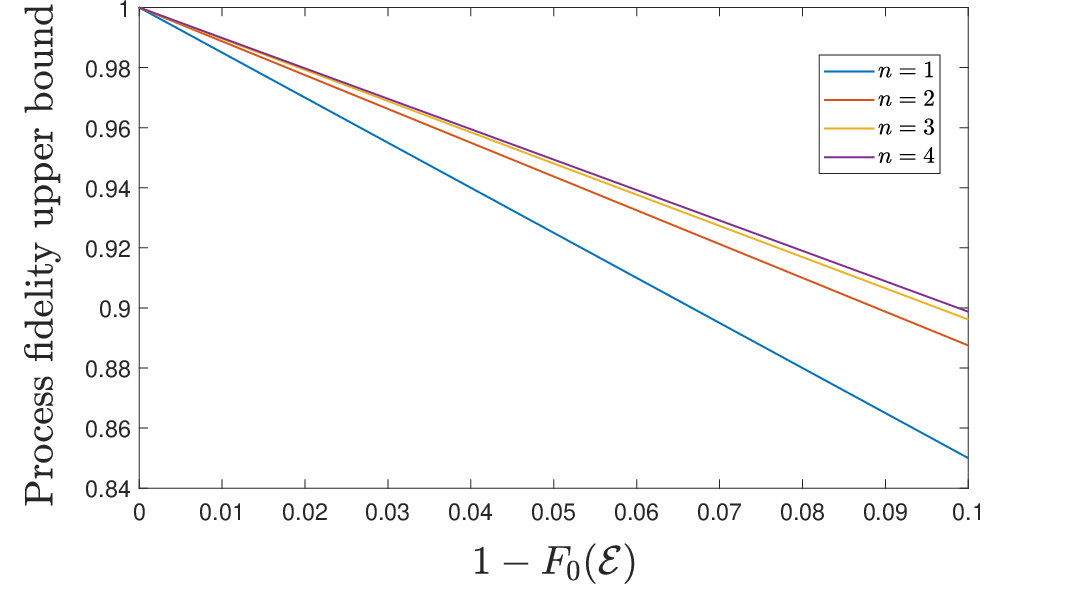
Similarly, a tight upper bound on $F(\mathcal{E})$ is given by solving

$\displaystyle\mathrm{Maximize}:\quad$	$\displaystyle\Tr(\chi\ket{\phi}\bra{\phi}),$
$\displaystyle\mathrm{Subject}\,\mathrm{to}:\quad$	$\displaystyle\Tr(\chi\Gamma)=dF_{0},$
	$\displaystyle\Tr_{2}(\chi)=I/d,$
	$\displaystyle\,\chi\geq 0.$	(21)

In this case, the solutions are strictly less than $F_{0}(\mathcal{E})$ , implying that the upper bound of $F(\mathcal{E})\leq F_{0}(\mathcal{E})$ in Th. 1 is not tight, but rather becomes an increasingly better approximation as $n$ increases. These results are shown in Fig 1. For $n=1$ , $\{\ket{\psi_k}\}_{k}$ is a 2-design and therefore $F_{0}(\mathcal{E})=F_{\mathrm{avg}}(\mathcal{E})$ , the average fidelity of $\mathcal{E}$ , given by Nielsen 2002

F_{\mathrm{avg}}(\mathcal{E})=\frac{dF(\mathcal{E})+1}{d+1}.

(22)

Therefore, for $n=1$ , the process fidelity is uniquely determined by the $0$ -fidelity, and is equal to the lower bound. For $n>1$ , the tight upper bound to the process fidelity converges to $F_{0}(\mathcal{E})$ as $n$ increases.

IV discussion

We have proven a lower bound on the process fidelity in terms of the $0$ -fidelity, namely $1-\frac{3}{2}(1-F_{0})\leq F$ , and by numerically solving an SDP for small $n$ conjecture that this bound is tight. The authors of Greenaway et al. 2021 numerically calculated $F_{0}(\mathcal{E})$ and $F(\mathcal{E})$ for an ensemble of random processes and concluded that $F_{0}(\mathcal{E})$ converges to $F(\mathcal{E})$ with increasing $n$ . While true for the ensemble of processes used in that simulation, if our conjecture holds, then the worst case process fidelity does not converge to the $0$ -fidelity with increasing $n$ . A description of the worst-case process is an open problem.

We have also computed the best-case process fidelity as the solution to an SDP. This solution does converge to the $0$ -fidelity with increasing $n$ , qualitatively matching the results from Greenaway et al. 2021, and improves upon the protocol in that work for estimating the process fidelity. Specifically, given an estimate of the $0$ -fidelity, the process fidelity may be estimated as the upper bound given by the SDP solution, rather than by the $0$ -fidelity itself.

Acknowledgements.

The author thanks Sean Greenaway for feedback on this manuscript while in preparation.

References

Greenaway et al. (2021) S. Greenaway, F. Sauvage, K. E. Khosla, and F. Mintert, Efficient assessment of process fidelity, Phys. Rev. Research 3, 033031 (2021).
Mayer and Knill (2018) K. Mayer and E. Knill, Quantum process fidelity bounds from sets of input states, Phys. Rev. A 98, 052326 (2018).
Renes et al. (2004) J. M. Renes, R. Blume-Kohout, A. J. Scott, and C. M. Caves, Symmetric informationally complete quantum measurements, Journal of Mathematical Physics 45, 2171–2180 (2004).
Nielsen (2002) M. A. Nielsen, A simple formula for the average gate fidelity of a quantum dynamical operation, Physics Letters A 303, 249–252 (2002).
Boyd and Vandenberghe (2004) S. Boyd and L. Vandenberghe, Convex Optimization (Cambridge University Press, USA, 2004).
Audenaert and De Moor (2002) K. Audenaert and B. De Moor, Optimizing completely positive maps using semidefinite programming, Phys. Rev. A 65, 030302 (2002).
Grant and Boyd (2014) M. Grant and S. Boyd, CVX: Matlab software for disciplined convex programming, version 2.1, http://cvxr.com/cvx (2014).

$\displaystyle M_{kk^{\prime}}$	$\displaystyle=\|\innerproduct{\psi_k}{\psi_{k'}}\|^{2}$
	$\displaystyle=\sum_{k_{1}k_{1}^{\prime}=1}^{4}\cdots\sum_{k_{n}k_{n}^{\prime}=1}^{4}\|\innerproduct{\psi_{k_1}}{\psi_{k_1'}}\|^{2}\cdots\|\innerproduct{\psi_{k_n}}{\psi_{k_n'}}\|^{2}$
	$\displaystyle=\prod_{i=1}^{n}\bigg(\sum_{k_{i}k_{i}^{\prime}=1}^{4}\|\innerproduct{\psi_{k_i}}{\psi_{k_i'}}\|^{2}\bigg).$	(15)