Deformed Schwarzschild horizons in second-order perturbation theory: mass, geometry, and teleology
Abstract
In recent years, gravitational-wave astronomy has motivated increasingly accurate perturbative studies of gravitational dynamics in compact binaries. This in turn has enabled more detailed analyses of the dynamical black holes in these systems. For example, Pound et al. [Phys. Rev. Lett. 124, 021101 (2020)] recently computed the surface area of a Schwarzschild black hole’s apparent horizon, perturbed by an orbiting body, to second order in the binary’s mass ratio. In this paper, we take that as the starting point for a comprehensive study of a perturbed Schwarzschild black hole’s apparent and event horizon at second perturbative order, deriving generic formulas for the first- and second-order corrections to the horizons’ radial profiles, surface areas, Hawking masses, and intrinsic curvatures. We find that the two horizons are remarkably similar, and that any teleological behavior of the event horizon is suppressed in several ways. Critically, we establish that at all orders, the perturbed event horizon in a small-mass-ratio binary is effectively localized in time. Even more pointedly, the event horizon is identical to the apparent horizon at linear order regardless of the source of perturbation, implying that the seemingly teleological “tidal lead”, previously observed in linearly perturbed event horizons, is not genuinely teleological in origin. The two horizons do generically differ at second order, but their Hawking masses remain identical, implying that the event horizon obeys the same energy-flux balance law as the apparent horizon. At least in the case of a binary system, the difference between their surface areas remains extremely small even in the late stages of inspiral. In the course of our analysis, we also numerically illustrate puzzling behaviour in the black hole’s motion around the binary’s center of mass.
I Introduction
I.1 Black holes in modern experimental physics
Over the past few decades, black holes have gone from hypothetical objects of theoretical interest to ubiquitous elements of observational astrophysics. LIGO and Virgo now regularly detect binary black hole mergers 3, and the Event Horizon Telescope has provided the first radio image of a black hole 5. Future technological advances will enable far more precise observations, both with next-generation gravitational-wave detectors 14; 50 and very-long-baseline radio interferometers 72; 85; 32. These will allow us to more stringently test whether the dark objects we observe are genuine black holes or some other exotic compact objects 21, and assuming they are black holes, whether they are accurately described by general relativity (GR).
In the near term, the most exacting measurements of black hole geometries will be made possible with the launch of the space-based gravitational-wave detector LISA in the early 2030s 30; 12. LISA will be sensitive to the merger of supermassive black holes, and the post-merger ringdown spectra from such systems will encode precise information about the nature of the final, merged object. Even more accurate measurements will be possible with LISA observations of extreme-mass-ratio inspirals (EMRIs), in which stellar-mass objects slowly spiral into massive black holes 6; 7. The companion in an EMRI acts as a probe of the massive black hole’s geometry, performing or more intricate orbits while in the LISA band, most or all of them within 10 Schwarzschild radii of the black hole. The emitted, long-lived waveforms have a rich harmonic structure carrying detailed information about the black hole (or exotic compact object) spacetime.
Measurements of this kind, with precise characterizations of deviations from GR’s black hole spacetimes, are possible because of the remarkable simplicity of isolated black holes in GR. In the post-merger ringdown phase, and through all phases of an EMRI, the spacetime can be approximated as that of an isolated, stationary black hole subject to small perturbations—either quasinormal modes after a merger or the perturbations generated by the companion in an EMRI. In GR, an isolated black hole is uniquely described by the Kerr-Newman metric, which is fully specified by its mass, spin, and charge. In an astrophysical scenario, a black hole is unlikely to carry charge, as any nonzero charge will be quickly neutralized. Therefore an astrophysical black hole in GR should be uniquely described as a Kerr black hole, which has a unique set of quasinormal modes and a unique multipole structure that are fully determined by the black hole’s mass and spin. By measuring the ringdown spectrum or the black hole’s multipole structure, we can detect small deviations from the Kerr geometry.
These prospects have motivated increasingly accurate theoretical studies of dynamically perturbed black holes in GR, moving beyond traditional linearized black hole perturbation theory onto second-order perturbation theory. There are ongoing efforts to calculate second-order effects in the ringdown of Kerr black holes 33; 49; 74 (building on earlier work in Ref. 20). And there is now a large body of work on EMRI models using gravitational self-force theory. In this method, the metric is expanded in powers of the binary’s mass ratio , where is the central black hole’s mass and the small companion’s. The perturbations effectively exert a self-force on the companion, accelerating it away from geodesic motion in the Kerr background. Surveys of self-force theory and EMRI modelling can be found in the recent reviews 11; 65.
It is well known that EMRI models sufficiently accurate for LISA science must be carried to second perturbative order in . Recently, Pound et al. reported the first calculation of a physical quantity at that order 64: the second-order contribution to the binding energy of quasicircular orbits around a Schwarzschild black hole. This calculation required a measurement of the Bondi mass of the binary, but also of the mass of the central black hole. In this paper, we take that calculation as the starting point for a more comprehensive study of perturbed Schwarzschild black holes at second order in perturbation theory. More specifically, we analyze the location and properties of a black hole’s perturbed horizon(s).
I.2 Black hole horizons
In principle, the defining feature of a black hole is its event horizon. However, event horizons are intrinsically teleological surfaces: we can only identify their precise location if we know the entire future history of the universe. This has motivated the development of alternative ways of characterizing dynamically evolving black holes based on locally identifiable criteria 39; 37; 41; 9; 17; 75; 48; 31; 43. The common characterization is via an apparent horizon or marginally outer trapped surface. Such a surface is defined in terms of the local-in-time, rather than global-in-time, behavior of null rays: given a slice of spacetime, an orientable, closed, spacelike 2-surface within the slice is a marginally outer trapped surface if future-directed null rays passing orthogonally outward through it have zero expansion. The apparent horizon is the outermost of these surfaces in the slice.
In GR, assuming appropriate energy conditions, the existence of an apparent horizon implies the presence of an event horizon, and the apparent horizon always either coincides with the event horizon or lies entirely inside the black hole. The converse is not true: the apparent horizon depends on one’s foliation of spacetime, and one can find pathological foliations in which no apparent horizon is present on a slice even though the slice cuts through the event horizon 86. However, for reasonable choices of foliation 8, the apparent horizon in a binary spacetime is found to be an excellent proxy for the event horizon except at moments very near merger 23.
Event and apparent horizons have been extensively studied and compared in numerical relativity; see, for example, Refs. 81; 82; 75; 23; 15; 62; 63. There is also a long history of research on linear perturbations of horizons. In recent years, perturbed horizons have been studied in Refs. 61; 84; 56; 57; 58, building on much earlier work in Refs. 38; 35; 36; 80; 70, for example. The series of papers 56; 57; 58 by O’Sullivan, Hughes, and Penna, in particular, have examined linearly perturbed black hole horizons specifically in EMRI scenarios at times significantly before the companion plunges into the black hole. A related line of work has examined linearly perturbed horizons in the specific case of a plunging companion 34; 27; 45; 26.
Our treatment extends these analyses to second perturbative order, restricted to a Schwarzschild background and largely following Poisson and collaborators’ treatment of the linear case in Refs. 61; 84. The extension to second order is necessary for the calculation of mechanical quantities in binaries, such as the binding energy in Ref. 64. But the extension is also interesting for one other major reason: in a binary inspiral, at times after merger or significantly before, it is precisely at second order that the apparent horizon (on a naturally chosen slicing) becomes distinguishable from the event horizon. It is also at this order that various definitions of the black hole’s properties begin to differ. For example, there is a natural, unambiguous measure of the black hole’s mass at linear order, but at second order one can define various nonequivalent measures of mass. In Ref. 64, Pound et al. specifically calculated the irreducible mass of the apparent horizon. Here, we show that the irreducible masses of the apparent and event horizon differ at second order, but that their Hawking mass (and Hawking-Hayward mass) remains identical.
I.3 Outline and summary
In Sec. II we begin by reviewing basic methods in black hole perturbation theory. We emphasize two-timescale expansions, which play an important role in our characterization of the event horizon in small-mass-ratio binaries. In Sec. III, we analyze the geometry of a generic 3-surface, foliated by spacelike 2-surfaces, near the background horizon; in later sections, this will be either the apparent or event horizon. We derive second-order perturbative formulas for the surface’s intrinsic metric, surface area, Hawking mass, and scalar curvature.
In Secs. IV and V, we then obtain second-order formulas for the location of the apparent and event horizon in terms of the perturbations of the metric. We show that in a small-mass-ratio binary, the event horizon can be localized in time except in the final phase of inspiral, when the companion transitions into a plunging orbit.
Section VI constructs simplified, gauge-invariant versions of the horizons’ area, mass, and curvature. Using these measures, we show that in a dynamical region of spacetime, the apparent and event horizon first differ from one another at second perturbative order. We derive simple formulas relating their radial profiles, surface areas, masses, and curvatures. As alluded to above, we show that despite their other differences, the two horizons have identical Hawking mass through second order.
Next, in Sec. VII, we specialize to the case of quasicircular inspirals. In that context, we demonstrate numerically that the difference between the horizons’ surface areas remains extremely small until near the innermost stable circular orbit, and we explain how the same is true for generic inspirals. We also examine the shape and location of the horizon at linear order, where we highlight two aspects. First, we emphasize that because the two horizons are identical at linear order, behavior that has previously been described as teleological must actually be entirely causal, and we suggest a nonteleological explanation for it. Second, we discuss a physically meaningful effect that has been omitted from previous depictions of the horizon at linear order: the motion of the black hole around the binary’s center of mass. We show that well-motivated definitions of the black hole’s “position” do not have the expected Newtonian limit for large orbital radii, suggesting a more robust analysis is required.
We conclude in Sec. VIII with a discussion of the implications of our results and their possible future developments. Among other applications, our results may be useful in sharpening the observed symmetry between quantities on the horizon and quantities at asymptotic infinity 68 and in concretely calculating black hole memory effects in realistic scenarios 40; 73.
Although motivated by EMRIs (and other small-mass-ratio systems such as intermediate-mass-ratio inspirals), most of our analysis applies to completely generic perturbations. Our only restriction is that in the intervals of time we consider, the number of null generators on the event horizon must remain fixed. This restriction is violated when additional generators join the horizon via caustics, as occurs when a body plunges into the black hole 34; 27; 45; 26. In the case of a binary inspiral, our analysis therefore fails in an interval containing the final plunge. However, for reasons explained in Sec. V, our analysis remains valid until shortly before the transition to plunge.
II Second-order perturbations of Schwarzschild spacetime
We begin in this section with an overview of the basic tools and conventions we use: second-order perturbation theory, the Schwarzschild metric, tensor spherical harmonics, and two-timescale expansions. Throughout the paper, we use geometric units with .
II.1 Perturbation theory through second order
We assume the spacetime metric depends on a small parameter , and we expand the metric up to second order,
| (1) |
where is the background metric and , are, respectively, the first- and second-order metric perturbations. In the context of a small-mass-ratio binary, will be the small mass ratio , but in most of our analysis we work with generic perturbations due to an unspecified source. It will sometimes be convenient to use the total perturbation
| (2) |
We focus on a region around the black hole, where we assume the spacetime is vacuum, satisfying the vacuum Einstein equation
| (3) |
Substituting the expansion (1) into the Ricci tensor, one obtains
| (4) |
where is linear in its argument and is quadratic in its argument; this expansion is reviewed in Appendix A. Equation (3) then becomes a sequence of equations, one at each order in :
| (5) | ||||
| (6) | ||||
| (7) |
The zeroth-order equation states that the background metric must be a vacuum solution. The first-order equation is the standard linearized Einstein equation. In the second-order equation, the second-order perturbation is sourced by quadratic combinations of the first-order perturbation.
In this paper, we will not focus our attention on solving these equations; we refer to Refs. 51; 18; 65 for descriptions of practical methods of obtaining solutions at first and second order in the case of a Schwarzschild background. Instead, taking the solution as a given, we analyze the effect the perturbations have on the black hole’s horizons. For the most part, as stated above, we allow the perturbation to be completely generic. However, at various points, we specialize to an important class of perturbations that depend on two disparate time scales, and in the final section of the paper we numerically compute properties of the horizon in the specific scenario of a quasicircular inspiral.
Most of our analysis will also leave the gauge of the metric perturbations unspecified. But one aspect of our calculations will make critical use of the gauge freedom within perturbation theory. In the perturbative context a gauge transformation corresponds to the infinitesimal coordinate transformation 19
| (8) |
under which the metric perturbations transform to
| (9) | ||||
| (10) |
Our conventions here follow Ref. 67.
II.2 Schwarzschild background
Throughout this paper, we take to be the Schwarzschild metric. We follow Refs. 51; 84 by writing the spacetime manifold as the Cartesian product , with charted by, for example, or , and charted by, for example, polar coordinates . The background 4-metric is then divided into an induced metric on each submanifold,
| (11) |
Here is the areal radius and is the metric on the unit sphere. On we exclusively use ingoing Eddington-Finkelstein coordinates, , such that
| (12) |
where . On we for the most part work covariantly, without specifying coordinates.
Our conventions for covariant derivatives and for raising and lowering indices are somewhat nonstandard. denotes the covariant derivative compatible with the exact metric, , and we use and its inverse, , to raise and lower Greek indices on nonperturbative quantities. and a semicolon denote the covariant derivative compatible with . For the most part, we avoid raising or lowering indices on perturbative quantities, but for the sake of brevity we occasionally use and its inverse, , for that purpose; in such instances, we explicitly warn the reader that we have done so. We also introduce as the covariant derivative compatible with the unit-sphere metric . We use and its inverse, , to raise and lower indices on quantities associated with , such as and (the Levi-Civita tensor associated with ). We do not use them to raise or lower capital Latin indices on other quantities.
We refer to Section II of Ref. 51 for additional useful identities related to the 2+2 split of the Schwarzschild metric.
II.3 Tensor spherical harmonics
Given Schwarzschild spacetime’s spherical symmetry, it is often convenient to expand quantities in spherical harmonics. With an appropriate choice of spherical basis functions, the Einstein equations separate into decoupled equations for each mode. In this paper, we assume that the metric perturbation is obtained mode by mode in this way. Such a harmonic decomposition will also allow us to easily solve the differential equations governing the location of the horizon and to evaluate various integrals over the horizon surface.
For the harmonics we adopt the conventions of Martel and Poisson 51. We start with the scalar spherical harmonics, , which satisfy the eigenvalue equation
| (13) |
where and is defined for any integer in Eq. (343). From the scalar harmonics we define the vector harmonics
| (14) | ||||
| (15) |
, are respectively referred to as even-parity and odd-parity vector harmonics. Finally we define the even- and odd-parity tensor harmonics
| (16) | ||||
| (17) |
which are both symmetric and trace-free with respect to .
These harmonics satisfy the orthogonality relations
| (18) | ||||
| (19) | ||||
| (20) | ||||
| (21) | ||||
| (22) | ||||
| (23) | ||||
| (24) |
Here is the surface element on the unit sphere, and we use to raise indices. An overbar denotes complex conjugation; the harmonics of all ranks satisfy identities of the form
| (25) |
It will be useful to split tensors on into their trace-free and traceful parts,
| (26) |
where and . Given this split, we expand the metric perturbations in spherical harmonics according to
| (27) | ||||
| (28) | ||||
| (29) | ||||
| (30) |
Each of the coefficients , , , and is a function of and .
Our second-order calculations will naturally involve products of functions on , and we will need to decompose such products into harmonics. As the simplest example, consider , which is (up to a factor of ) the scalar monopole mode of the product . Expanding each function in harmonics, as and , and using Eqs. (18) and (25), we obtain
| (31) |
where we have used the fact that for any real-valued function . The analogous rule applies for integrals of the form and . In Appendix B we describe our procedure for evaluating more general integrals.
II.4 Two-timescale expansion
Most of our analysis utilizes regular perturbation theory, in which the coefficients in Eq. (1) are independent of the small parameter . However, at various points we adopt an expansion that is better suited to a small-mass-ratio binary: a two-timescale expansion. We refer to textbooks on singular perturbation theory for introductions to the method (e.g., 47). In the particular context of an inspiral into a black hole, the use of the method is inspired by the fact that during the inspiral, the system evolves on two distinct timescales: the short orbital timescale associated with the companion’s orbital frequency ; and the long radiation-reaction time , over which the orbital frequencies evolve due to gravitational-wave emission. A two-timescale expansion allows us to maintain accuracy on both timescales, while regular perturbation theory would break down well before a radiation-reaction time 65.
Concretely, an orbiting, nonspinning body in the equatorial plane of Schwarzschild spacetime has two independent frequencies, and , associated with radial and azimuthal motion. Specialized to a region around the horizon, the two-timescale ansatz for the metric is then
| (32) |
where , and the sum runs over all pairs of integers . In this expansion we have introduced the slow time variable and the orbital phases , which are given by
| (33) |
or equivalently, ; the unspecified lower limit in Eq. (33) represents an arbitrary choice of initial condition. The metric perturbations in Eq. (32) hence have the character of a sum of slowly varying amplitudes multiplied by rapidly varying phase factors. We refer to Refs. 52; 65 for more detailed descriptions of such two-timescale expansions of the metric, which are further developments of Hinderer and Flanagan’s seminal work on the two-timescale expansion of inspiral orbits 44. Such an approximation should be uniformly accurate until a time shortly before the inspiraling body transitions to a plunging orbit 54; we describe that cutoff in Sec. V.
Treated as a function of the coordinates on , the coefficients of in the expansion (32) depend on , meaning (32) is not a Taylor series around ; this is a defining characteristic of singular perturbation theory 66. However, the dependence on comes in a circumscribed form that allows us to solve the field equations through any desired order on the radiation-reaction timescale. We can also view Eq. (32) as a regular Taylor expansion of a field on a higher-dimensional manifold charted by . is embedded into this larger manifold with a map defined by . After performing the ordinary Taylor expansion of the function on , we then pull it back to its restriction on the physical spacetime manifold .
Quantities on the horizon inherit the metric’s two-timescale form, which has several important consequences. First, derivatives involve terms that are suppressed by one order in . To see this, let be a field on , and let be its restriction to , such that . The derivative of then becomes
| (34) |
The first term, which characterizes the field’s slow evolution, will be demoted to the next order, such that if appears on the horizon at first perturbative order, for example, then its derivative will contribute to second-order quantities on the horizon. For notational simplicity, we will not distinguish between and its pullback .
The second consequence of the two-timescale expansion is that it transforms differential equations in into algebraic ones. Suppose we have a differential equation governing a quantity’s behavior on the horizon, of the form
| (35) |
If we expand in the Fourier series and , then at leading order Eq. (35) becomes
| (36) |
where . This kind of transformation is one of the key utilities of the two-timescale expansion. For example, it puts the Einstein field equations (6) into precisely the same form they would have in a standard frequency-domain treatment, while correctly capturing the system’s slow evolution.
Transforming differential equations in this way implicitly localizes them in time: rather than having to integrate over from some initial condition, we algebraically determine the solution at a given value of slow time . This is especially relevant for the event horizon, which is inherently a nonlocal-in-time surface that depends on the spacetime’s distant future. The underlying reason for this localization in time is that integrals over large ranges of collapse to local-in- quantities when the integral contains multiple time scales. For example, consider the integral , which extends from the present time into the infinite future. If vanishes when , then we can repeatedly integrate by parts to obtain11 1 For resonant modes that pass through for some value of 83, this approximation breaks down. The integral should in that case be approximated using the stationary-phase approximation 65. For simplicity we exclude resonances from our analysis.
| (37) |
Depending on the behavior of and in the far future, this approximation can be carried to arbitrary order in , making nonlocal effects arbitrarily small. We will see in Sec. V how this type of approximation applies to the location of the event horizon.
Because it cleanly separates slow and fast evolution, a two-timescale expansion also allows us to unambiguously identify the time average of a quantity as the zero mode in its fast-time Fourier series:
| (38) |
This will enable us to characterize the black hole’s average evolution, discarding fluctuations on the orbital timescale.
Finally, we note that the mode number is precisely the azimuthal mode number . This is because, due to the background spacetime’s axisymmetry, the small body’s stress-energy can only depend on and in the combination , and the metric perturbations inherit that dependence; see Sec. 7.1 of Ref. 65. As a consequence, we can write the expansion (32) in the form
| (39) |
For the quasicircular orbits we consider in Sec. VII, this reduces to
| (40) |
III Geometry of a perturbed horizon
Before considering the apparent horizon and event horizon in detail, we begin by describing the geometry of a generic 3-surface close to the background horizon, which may be either of the two horizons. This serves to set our notation and to present formulas that will be common to both horizons.
Over the course of the section, we introduce a convenient basis of vectors and the induced metric on the surface, and we then derive perturbative formulas for the horizon’s surface area and intrinsic curvature. We conclude by showing the consistency between our formulas for the area and curvature, as dictated by the Gauss-Bonnet theorem.
III.1 Embedding and induced metric
As coordinates on , we use the extrinsic coordinates . is then described by an embedding
| (41) |
We assume that the perturbed horizon’s radial profile can be written as an expansion around the background horizon radius:
| (42) |
The perturbations will depend on whether is the apparent horizon or the event horizon. In Secs. IV and V, we express in terms of the metric perturbations in each of the two cases.
The embedding (41) defines a basis of vectors fields tangent to ,
| (43) |
In terms of these tangent vectors, the induced metric on is
| (44) |
However, we will be more interested in the foliation of into spacelike slices of constant , , on which we use coordinates . The basis of vectors tangent to is
| (45) |
and the induced metric on is
| (46) |
If we substitute the expanded metric (1), we can write this as
| (47) |
where and for . The components of are functions of the coordinates on , and they inherit an additional parametric dependence on .
We do not provide more explicit expressions for the coefficients because we ultimately perform an additional expansion of them. This second expansion is called for because Eq. (47) is written in terms of tensors at points on . It will generally be more useful to expand all such tensors around their values on the background horizon. By substituting the expansion (42), we can expand any tensor’s components on as
| (48) |
where derivatives of on the right are evaluated at . Geometrically, this represents an expansion of the pullback , where maps points on the background horizon to points on the perturbed horizon. The pullback can be expressed in terms of Lie derivatives as with and .
Performing such an expansion for the induced metric, we find
| (49) |
where
| (50) | ||||
| (51) |
All quantities on the right are evaluated at . The inverse metric is then
| (52) |
Similarly, the basis vectors (45) on become
| (53) |
with
| (54) | ||||
| (55) | ||||
| (56) |
Later calculations will require the expansion of these quantities in spherical harmonics. We write the radial perturbations as
| (57) |
and we write as
| (58a) | ||||
| (58b) | ||||
The coefficients and are straightforwardly expressed in terms of the coefficients in the harmonic expansions of and . At first order,
| (59a) | ||||
| (59b) | ||||
At second order, we must decompose products of harmonics into pure harmonics, as described in Appendix B. The result is
| (60a) | ||||
| (60b) | ||||
where the symbols are given in Eq. (B), and their -dependent coefficients are given by
| (61a) | ||||
| (61b) | ||||
| (61c) | ||||
| (61d) | ||||
| (61e) | ||||
Here we use the compact notation described in Appendix C. These formulas will substantially collapse in Sec. VI.
III.2 Null basis vectors
On each slice we introduce a pair of future-directed null vectors and . Both are orthogonal to , satisfying
| (62) | ||||
| (63) |
is chosen to point outward from , toward the horizon’s exterior, and to point inward, into the black hole’s interior. Together with , these vectors form a basis for 4-vectors at points on . In the case of the event horizon, will be the tangent vector of the horizon generators; in the case of the apparent horizon, will not, generically, be tangent to the surface .
In both cases, we normalize such that , and we scale such that it satisfies
| (64) |
The metric can then be written as
| (65) |
where , and the metric’s inverse can be written as
| (66) |
Given the normalization , the orthonormality conditions (62)–(64) uniquely determine and in terms of , , and . Assuming expansions of the form
| (67) |
and analogous for , we can solve the orthonormality equations for the coefficients at each order. At leading order,
| (68) | ||||
| (69) |
We again elide explicit expressions for and to higher order, instead presenting results for the re-expansions around the background horizon,
| (70) | ||||
| (71) |
The leading terms in these expansions are
| (72) | ||||
| (73) |
The first subleading terms are
| (74) | ||||
| (75) |
where all terms on the right are evaluated at . The second-order terms in are
| (76a) | ||||
| (76b) | ||||
| (76c) | ||||
In our analysis we will not require the explicit expressions for beyond , but we use them as a consistency check in some of our calculations. We include them here for completeness:
| (77a) | ||||
| (77b) | ||||
| (77c) | ||||
III.3 Surface area and mass
The surface area of the slice is given by the integral
| (78) |
where is the determinant of the 2-metric . By substituting the expansion (49), we can write the surface element as an expansion
| (79) |
where the subleading terms are
| (80) | ||||
| (81) |
We omit breves on the quantities for notational simplicity.
To evaluate the integral, we appeal to the harmonic expansions (58), orthogonality relations (18)-(24), and the identity . The result is
| (82) |
where
| (83) | ||||
| (84) |
The area of the horizon provides a measure of the black hole’s irreducible mass,
| (85) |
sometimes called the Christodoulou mass. As its name suggests, the irreducible mass cannot be lowered by any (classical) physical process. Historically, this definition arose from the case of a Kerr black hole 22, from which some amount of energy can be extracted via the Penrose process 59. After substitution of the expansion (82), the irreducible mass reads
| (86) |
where .
The irreducible mass is closely related to another quasilocal measure of mass: the Hawking mass 42; 46,
| (87) |
Here and are the expansion scalars associated with and , respectively. Unlike irreducible mass, which simply measures the area of a surface, the Hawking mass directly involves the gravitational pull at the surface, as characterized by the expansion or contraction of the two null congruences. In our case, will always be negative, while will be either zero or positive. An apparent horizon is defined by , meaning for an apparent horizon. But for the event horizon , meaning provides a simple alternative measure of the mass within the event horizon.
We return to these quantities in later sections.
III.4 Intrinsic curvature
Since is a 2-surface, its intrinsic curvature tensor can be written in terms of its Ricci scalar as
| (88) |
where we use a calligraphic to avoid confusion with the curvature tensor of the unit two-sphere. In this section, we derive a perturbative formula for through second order in ,
| (89) |
To carry out the expansion, we consider the metric with . The scalar curvature of this metric can be expanded in powers of as
| (90) |
following the notation in Appendix A. Explicitly, Eqs. (329) and (330) (with ) reduce to
| (91) | ||||
| (92) |
where . Letting , we then have
| (93) | ||||
| (94) |
Decomposing these quantities into harmonics, we find at first order
| (95) |
where . This agrees with the result from Vega et al. 84. Decomposing the quadratic quantity requires decompositions of products of angular functions into scalar harmonics. We perform that decomposition following the method outlined in Appendix B, eventually arriving at
| (96) |
where the symbols are given by Eq. (B) and the functions are given in Eq. (356).
III.5 Gauss-Bonnet theorem
For any closed two-dimensional Riemannian surface , the Gauss-Bonnet theorem states that the surface’s total curvature is related to its Euler characteristic according to
| (97) |
where is the area element on . Applied to our case, where the surface has the topology of a 2-sphere, the equality becomes
| (98) |
In this section, we use this identity as a consistency check of our results for the surface area and intrinsic curvature.
Substituting the expansions (79) and (89) into the left-hand side of the identity, we obtain
| (99) |
Here we have used . Equating this expansion to the right-hand side of Eq. (98) yields an equation at each order in ,
| (100) | ||||
| (101) |
The right-hand side of Eq. (100) evaluates to
| (102a) | ||||
| (102b) | ||||
where we have appealed to Eq. (95). Comparing this result to Eq. (83) for , we see that Eq. (100) is satisfied.
Next, the right-hand side of Eq. (101) evaluates to
| (103a) | ||||
| (103b) | ||||
To avoid stacking bars on top of breves, here we let an overbar denote the complex conjugate of a quantity that otherwise would carry a breve. The monopole mode of the quadratic term in Eq. (96) can be simplified to
| (104) |
Substituting this into Eq. (103) and comparing the result to Eq. (84) for , we find that Eq. (101) is satisfied.
IV Apparent horizon
We now consider the apparent horizon. In this section, we obtain a perturbative description of the horizon’s radial profile in terms of the metric perturbation. The horizon’s area, mass, and curvature are then given by the generic formulas of the previous section. Our notation and conventions largely follow the textbook of Poisson 60.
IV.1 Specification of the horizon
We first foliate the spacetime with surfaces of constant . On each , the apparent horizon is a closed spatial 2-surface; this now plays the role of from our generic treatment.22 2 An apparent horizon is more commonly described as a 2-surface embedded in a spatial hypersurface. One can always find some foliation into spacelike 3-surfaces for some time function such that the apparent horizon in is identical to . The construction in this section is indifferent to which of these submanifolds the apparent horizon is embedded into, but the foliation into surfaces labelled by is most natural in our perturbative context. On this surface, we have the two future-directed null vector fields, and , that are orthogonal to . To illuminate the definition of the apparent horizon, we extend and off of by taking them to be the tangent vector fields to congruences of null curves, and , respectively. The choice of these congruences is arbitrary; the curves making up () may be accelerating and nonaffinely parametrized, for example, so long as they are tangent to () at . The congruences’ kinematics at are described by the 2-tensors
| (105) | ||||
| (106) |
and their expansion scalars are
| (107) | |||
| (108) |
A spatial 2-surface in is a trapped surface if and , and it is marginally trapped if and . The apparent horizon is the outermost marginally trapped surface in . The collection of apparent horizons forms a 3-surface , which we also refer to as the apparent horizon. This plays the role of from our generic treatment. is spacelike in dynamical regions of spacetime; it is then a dynamical horizon in the sense of Ashtekar 9. It is null in stationary regions of spacetime; it is then an isolated horizon 9.
will always be negative when vanishes, allowing us to calculate only . The equation determining the apparent horizon’s location is then
| (109) |
One might imagine there being multiple solutions to this equation, requiring us to find the outermost one. ( would represent a dynamical or isolated horizon in any case, but not an apparent horizon.) However, in our context of a perturbed Schwarzschild black hole, we will find that Eq. (109) specifies a unique surface near the background horizon.
Before calculating the expansion, we note that and only involve derivatives of and within . Therefore although it can be helpful to think of the expansion scalars in terms of congruences of curves, they are actually fully specified by the basis vectors and on . They do not depend on the complete congruences, nor do they depend on the vectors being tangent to geodesics. In the literature one more commonly sees the simplified form , which holds for an affinely parametrized congruence. Generically, for accelerating, nonaffinely parameterized curves, the curves in satisfy
| (110) |
on , for some and . [There is no component along because the contraction with must vanish: .] Using Eq. (66), we can therefore write the expansion as
| (111) |
If the curves are affinely parametrized, regardless of whether they are geodesics or accelerated, this simplifies to the standard expression . However, because these expressions require an extension off of , we instead exclusively use Eq. (107).
IV.2 Radial profile of the horizon
In this section, we solve Eq. (109) to find the horizon’s radial profile.
We first write Eq. (107) in terms of background quantities and perturbative quantities. The tensor defined in Eq. (105) can be written as
| (112) |
Here is given by Eq. (319). In evaluating Eq. (112), we first take derivatives at the coordinate location of the perturbed horizon, , using expansions of the form (67) for the null vector and applying radial derivatives as . After that, we carry out expansions of the form (48), using Eqs. (53) and (70). Finally, when evaluating the contraction , we use Eq. (52).
As a check of our calculation, we have also performed the operations in an alternative order, leaving and at , using the form Eq. (47) for , and then performing the expansion (48) at the level of the scalar quantity . As an additional check, we have also used the alternative form to obtain the same result.
In all variations of the calculation, we arrive at
| (113) |
The zeroth-order term identically vanishes because the background horizon has zero expansion in the background spacetime. The first-order term is
| (114) |
The second-order term is given in Eq. (357).
To solve the equations , we expand all quantities in tensorial spherical harmonics using Eqs. (27)–(30) and (57) and then decompose into scalar-harmonic modes . After appealing to the identity (13) and the definitions (14) and (15), we immediately find
| (115) |
The solution to is therefore
| (116) |
All quantities on the right are evaluated at .
Finding requires decomposing products of tensorial harmonics into modes. As in our decompositions in Sec. III, our method of decomposing such products is described in Appendix B. Our calculation in this section in particular utilizes the identities (351)–(354). The result is an equation of the form
| (117) |
where the symbols are defined in Eq. (B) and the functions are given in Eq. (358). The solution to is therefore
| (118) |
IV.3 Surface area, mass, and intrinsic curvature
Given the perturbations (116) and (118) to the horizon’s radial profile, we can compute the intrinsic metric (49) using (58) with Eqs. (59) and (60). From the intrinsic metric we can then compute the surface area, mass, and intrinsic curvature using Eq. (82), Eq. (86), and Eq. (89) [with Eqs. (95) and (96)]. Because on the apparent horizon, the horizon’s Hawking mass (87) is identical to its irreducible mass.
The surface area and the mass both require the monopole mode of . For , Eqs. (116) and (118) reduce to
| (119) | ||||
| (120) |
The explicit expression for is given in Eq. (C).
The surface area and mass at first order are easily evaluated. Note that an vacuum perturbation is necessarily a perturbation toward another Schwarzschild solution, which (with an appropriate choice of gauge) we can write as
| (121) |
for some . Therefore the correction to the horizon radius, as given in Eq. (119), is
| (122) |
With Eqs. (83) and (59), this implies that the correction to the surface area is
| (123) |
and the correction to the black hole mass, given in terms of the surface area in Eq. (86), is
| (124) |
(noting again that the Hawking and irreducible mass are necessarily identical for the apparent horizon). can also be invariantly defined as the Abbott-Deser mass contained in 2; 25; for linear perturbations of Schwarzschild spacetime, all sensible definitions of mass agree.
In the context of a binary inspiral, where the two-timescale expansion (32) applies, all the same results hold true except that (i) the black hole’s gradual absorption of energy requires that becomes a function of 52, and (ii) picks up an additional slow-time derivative term,
| (125) |
coming from the chain rule (34) applied to the derivative in Eq. (116). After this correction is accounted for, all derivatives are then to be interpreted as the fast-time derivative . The correction (125) plays an important role in our comparison of the apparent and event horizons in later sections.
We defer any evaluation of the scalar curvature or the second-order expressions to Sec. VI, where they will be substantially simplified.
V Event horizon
In this section, we obtain a perturbative description of the event horizon’s radial profile in terms of the metric perturbation, following the method of Refs. 61; 84. We then show that in the context of a two-timescale expansion, the event horizon is effectively localized in time. At the end of the section we begin our comparison of the two horizons.
V.1 Specification of the horizon
A black hole is intrinsically a nonlocal object. It is formally defined as a region that is causally disconnected from future null infinity :
| (126) |
where is the causal past of . Its event horizon is the boundary of this region,
| (127) |
We denote the horizon as to indicate that it is perturbatively close to the background spacetime’s future horizon rather than its past horizon. here plays the role of our generic surface from Sec. III, and cuts of constant , , play the role of . The definition (127) implies that the location of the event horizon at a given advanced time depends on the entire future history of the spacetime.
To locate the horizon in practice, we first note that because it is a null surface, it is necessarily generated by a family of null geodesics. Each of these geodesics can be parametrized with advanced time , such that it has coordinates . Since the curve must be within the horizon surface, which we parametrized as , we can write as
| (128) |
Its tangent vector is then given by
| (129) |
where
| (130) | ||||
| (131) |
and . This implies , and
| (132) |
Because it is tangent to the null surface’s generators, must also be orthogonal to the horizon. This means satisfies all the same orthonormality conditions as in our generic treatment in Sec. III: , (62), and (64). Therefore on each cut of the horizon, , is uniquely determined as a function of and exactly as in the generic treatment. So in particular, (or equivalently, ) is given in terms of by Eq. (70) with the component of Eq. (74) and with (76c). However, rather than using Eqs. (74) and (76b) for , we can instead use the form (132). The null condition then becomes a first-order differential equation for the radial profile as a function of .
So far, this description only specifies that is a null surface. To specify which null surface it is, we need to impose teleological boundary conditions. We assume that in the distant future, the spacetime settles to a stationary, Kerr black hole. In that stationary state, the event horizon has the standard radial profile of the Kerr horizon. Our teleological condition on is that when , reduces to the Kerr horizon’s radial profile. In other words, the integral curves of must start in the distant future as the generators of the Kerr horizon and then be evolved backward in time from that end state. In Sec. V.3 we comment on some subtleties in this condition.
V.2 Radial profile of the horizon
We obtain evolution equations for by expanding Eq. (132) in the form (70), which implies
| (133) | ||||
| (134) |
The other components are described above.
Substituting our expansion of into , we find
| (135) |
and
| (136) |
where all quantities on the right are evaluated at .
We can write these equations in the common form
| (137) |
where we have introduced , the surface gravity of the unperturbed Schwarzschild black hole. Expanding the equations in scalar spherical harmonics, we obtain
| (138) |
The first-order driving term is immediately found to be
| (139) |
Calculating the modes of the second-order driving term requires decomposing products of vector harmonics into single scalar harmonics; as stated previously, this is described in Appendix B. The result is
| (140) |
with
| (141) | ||||
| (142) |
Here we use the compact notation described in Appendix C, and we additionally define .
The differential equations (138) have the teleological solutions
| (143) |
Under the assumption that can be treated as effectively constant after some late time , the solution (143) correctly becomes the constant for all . If we adopted a causal solution instead, the solution would grow exponentially as at late times.
To exactly evaluate the integral (143) at a given time , we need to know for all . This requires simulating the spacetime’s entire evolution, allowing it to settle to a stationary state, and only then finding the location of the horizon at earlier times.
V.3 Timescales and temporal localization on the horizon(s)
In Refs. 61; 84, Poisson and collaborators show that under certain circumstances, the teleological effects on the horizon’s location are strongly suppressed, and the horizon is effectively localized in time. In this section, we review that argument, recall why it does not apply to binaries, and then apply a variant of it to show that in a small-mass-ratio inspiral, the timescales are such that the horizon is always temporally localized except in an interval of advanced time around the final plunge.
The essential idea of the localization is that the exponential factor in Eq. (143) exponentially suppresses the effects of the distant future. Integrating by parts, as we did to obtain Eq. (37), we can express Eq. (143) as
| (144a) | ||||
| (144b) | ||||
This is a sensible approximation if the characteristic frequency of is much smaller than .
In a binary inspiral, the frequencies can be much larger than , meaning this approximation is inappropriate. However, we can nevertheless develop a similar localization approximation. We do this in two steps: First, we show that the far future has negligible impact on the location of the horizon at times significantly before plunge. Second, we show that during the inspiral phase, the approximations (37) and (144) can be combined to localize the horizon.
Generically, a small-mass-ratio binary evolves through four phases 79: the slow inspiral; the transition to plunge when the companion approaches the innermost stable circular orbit (or more generically, when it approaches the separatrix between stable and plunge orbits 76); the plunge itself; and finally, the post-merger ringdown, when the black hole settles to a stationary, Kerr state. Each of these phases has an associated evolution timescale. The inspiral is characterized by the orbital timescale and the long radiation-reaction time . The transition to plunge is characterized again by the orbital timescale, but also by the transition timescale 54, as the orbit more rapidly evolves during the transition phase. The plunge itself occurs rapidly, on the timescale . Finally, the ringdown phase itself has two types of evolution: the rapid exponential decay of the black hole’s quasinormal modes 13, and the late-time tails 71 that decay with a power law along the horizon 10.
We now consider a time in the inspiral phase. Our first goal is to show that all the later phases have negligible impact on the location of the horizon at time . In the process, we find an estimate of the cutoff time where our treatment breaks down.
We first split the integral (143) into four segments corresponding to the different phases of the system, , where the labels refer respectively to transition, , to plunge, , and to ringdown, . We then consider these one by one, starting with the integral over the transition regime, which we write as
| (145) |
To ensure that we can neglect this integral, we require it to be much smaller than , such that the contribution for is negligible compared to the effects that we calculate.
Although the transition is rapid compared to the inspiral, it is slow compared to the orbital period, and throughout the transition we can adopt an adapted two-timescale form for the forcing function, , where . (We suppress indices for the remainder of this discussion; the approximations can be carried out at the level of the sum of modes or at the level of individual modes). For each mode, the integral then has the form
| (146) |
where . This function has the properties
| (147) | ||||
| (148) |
Repeatedly integrating by parts, we obtain
| (149) |
The quantity in brackets is order 1. Therefore, for to be much smaller than , we need . This relation translates into a relation for :
| (150) |
So we conclude that during the inspiral phase, we may neglect the impact of the transition phase so long as we restrict ourselves to advanced times satisfying Eq. (150). Note that this is a far smaller time interval than the radiation-reaction time, implying that the companion can get very near to the transition before the transition’s influence on the horizon is felt.
Next, we consider the integral over the plunge phase, which can be written as
| (151) |
During the plunge, the timescale on which varies is , implying the contribution from the integral is of order 1, excluding the exponential factor outside it. Therefore the cutoff (150) ensures that is much smaller than .
The same argument applies to the integral over the ringdown phase,
| (152) |
The cutoff (150) ensures that is much smaller than .
We have now shown that all the future phases have negligible impact on the horizon during the inspiral phase. We have only one remaining integral,
| (153) |
which we are able to localize in time using the now-familiar integration by parts. If we expand the forcing function in two-timescale form, as , then for each mode , we have an integral
| (154) |
where we have defined
| (155) |
This function has the properties
| (156) | ||||
| (157) |
If we now repeatedly integrate by parts while appealing to these properties and the cutoff (150), we obtain the approximation
| (158) |
As promised, although neither of the approximations (37) or (144) is alone accurate, a variant which combines them does provide an accurate approximation that localizes the teleological integral. The oscillations in the two-timescale approximation approximately average out over the integration domain, while the exponential decay eliminates the impact of the very far future. In the case of quasistationary modes, with , the approximation (V.3) simply reduces to Eq. (144), but for these modes is the slowly varying function , meaning each derivative in Eq. (144) comes with a power of .
By substituting Eq. (139) for , we now obtain the temporally localized perturbations to the event horizon’s radius:
| (159) |
and
| (160) |
These formulas can be made more explicit using
| (161) |
For quasistationary modes, these results give the slowly evolving average corrections to the horizon radius:
| (162) | ||||
| (163) |
where we recall the definition (38) of the average of a two-timescale function.
Before moving to the next section, we comment on how applicable our results are to other scenarios and phases. In this section we have focused on the location of the horizon in the inspiral phase. The same arguments apply to the transition phase, and we expect the event horizon to remain localized for a significant portion of the transition (although, to our knowledge, there has not yet been a complete multiscale treatment of the transition phase, including the metric perturbation in addition to the companion’s trajectory).
In the plunge phase, the horizon is not localizable, and moreover, much of our analysis throughout this paper breaks down. As the companion approaches the black hole, additional generators join the horizon 34; 27; 45; 26. The caustics they form create a cusp on the horizon. Although our treatment of individual generators remains valid in that case, the horizon does not have a smooth induced metric, and the generic treatment in Sec. III becomes invalid. The additional generators that join the horizon can also begin from a great distance away from it. The cusp extends into the infinite past on the horizon, suggesting one should worry that this spoils our treatment of the inspiral phase as well. However, the cusp is exponentially suppressed in the same way as other effects discussed in this section, and we can safely ignore it.
Finally, in the ringdown phase, our generic treatment of the horizons apply perfectly well. But since quasinormal modes have frequencies and decay rates comparable to , there is no temporal localization in the early stage of the ringdown. At late times, if the power-law tails die out on a much larger timescale than , then Eq. (144) should apply.
V.4 Surface area, mass, and intrinsic curvature
Just as in the case of the apparent horizon, given the perturbations (143) to the horizon’s radial profile, or (159) and (160) in an inspiral, we can compute the intrinsic metric (49) using (58) with Eqs. (59) and (60). From the intrinsic metric we can then compute the surface area, irreducible and Hawking mass, and intrinsic curvature using Eq. (82), Eqs. (86) and (87), and Eq. (89) [with Eqs. (95) and (96)].
The surface area and masses require the term in the horizon radius, . These are obtained from the forcing functions in Eqs. (139) and (V.2), which read
| (164) | ||||
| (165) |
Like we did for the apparent horizon, we can quickly obtain the surface area and mass at first order. Using Eq. (121) for in Eq. (143), we recover ; this is identical to the result (122) for the apparent horizon. The same can also be obtained from Eq. (162), noting that a vacuum monopole perturbation can always be written in a gauge in which it is a pure mode. Equations (83) and (86) then imply and , just as for the apparent horizon.
Unlike the apparent horizon, the event horizon’s Hawking mass (87) differs from its irreducible mass. However, the difference only enters at second order. At first order, the expansion vanishes 61; 84; we reproduce this result in the next section. We therefore have . The expansion scalar for the ingoing null vector is easily calculated to be . Therefore the Hawking mass of the event horizon is
| (166) |
We simplify this formula in the next section. There, we make a thorough comparison of the two horizons. To preface that comparison, we note that because , the event horizon is in fact identical to the apparent horizon at first order. As alluded to in the Introduction, they only begin to differ at second order.
VI Gauge fixing and invariant properties of the horizons
So far our calculations have not specified a choice of gauge. At first order, it is straightforward to show that quantities such as the black hole mass are invariant under the linear transformation (9). Moreover, the horizons themselves are invariant 3-surfaces. However, their foliations into surfaces of constant are inherently gauge dependent. Even given some foliation, a transformation within each 2-surface does not leave all our quantities invariant. As a simple example, consider the horizon’s scalar curvature. Under a gauge transformation generated by a vector that is tangent to , the first-order correction to the scalar curvature, , transforms as . Since the zeroth-order curvature is constant on the horizon, this implies that is invariant under these transformations. However, then transforms as . Since is not constant, is not invariant.
Quantities such as the horizon area and mass of are invariant under transformations within , since they are defined as integrals over . But they are not invariant under a transformation that alters the foliation. And analyzing how they transform is nontrivial because we have described the horizons’ locations using gauge-dependent parametrizations .
In this section, we construct invariant quantities associated with the curvature, area, and mass of the horizons. Our procedure for constructing these invariant quantities is based on gauge fixing: we write all variables in terms of the transformation to a preferred, fully fixed gauge in which the perturbed event horizon remains at the coordinate location . Such a gauge is described as horizon locking 84. Our procedure also gives invariant geometrical meaning to our foliation and to the apparent horizon’s location relative to the event horizon. At the end of the section, we are able to isolate the precise differences between the two horizons.
Since we will be comparing between quantities on and , in this section we explicitly add a “” or “” label to quantities such as , , and .
VI.1 Gauge-fixed metric perturbations
Referring to Eqs. (9) and (10), we define the gauge-fixed metric perturbations to be
| (167) | ||||
| (168) |
In terms of Eddington-Finkelstein components, these equations read
| (169a) | ||||
| (169b) | ||||
| (169c) | ||||
| (169d) | ||||
| (169e) | ||||
| (169f) | ||||
| (169g) | ||||
The components of are given by the same equations with the replacements and , where
| (170) |
In these expressions, is the unique vector that transforms from the “user gauge” (whichever gauge one happens to use to solve the field equations) to the fixed gauge. By imposing geometrical conditions on , we will express explicitly in terms of . This process will be expedited by introducing the tensor-harmonic expansion
| (171) | ||||
| (172) |
Once is determined, the quantities will then be given by simple formulas in terms of . These formulas will be gauge invariant: takes the same value regardless of the gauge that is in. The horizons’ surface area, curvature, and mass will then be written in terms of manifestly invariant quantities with clear geometrical meanings.
Finally, to facilitate this gauge-fixing procedure in the case of a binary inspiral, we introduce a division of each field into its quasistationary and oscillatory pieces,
| (173) | ||||
| (174) | ||||
| (175) | ||||
| (176) |
Each of the oscillatory quantities has an expansion of the form
| (177) |
which excludes the quasistationary, terms from expansions of the form (32). When substituting these two-timescale forms into Eqs. (167)–(168), the first-order equation becomes (169) with . A derivative acting on dependence is demoted to second order. We can absorb those terms into a redefinition of :
| (178a) | ||||
| (178b) | ||||
| (178c) | ||||
with other components unchanged. All other derivatives in the second-order expressions are then replaced with .
VI.2 Gauge fixing
VI.2.1 Horizon locking
We first impose the condition that the event horizon of the perturbed spacetime lies at the coordinate radius . An example of a gauge condition that enforces this is the Killing gauge 84, defined by for all . For reasons we describe momentarily, we impose a slight variant of that condition. We first impose
| (179) | ||||
| (180) |
Here indicates evaluation at ; we do not require these conditions to hold at any points away from . Examining Eq. (135), we see that in a gauge satisfying Eq. (179), the leading perturbation to the event horizon’s radius, , vanishes. Given this, examining Eq. (V.2), we see that in a gauge satisfying both Eqs. (179) and (180), the second-order perturbation likewise vanishes. In both cases, we assume the teleological solution for , which rules out the nontrivial homogeneous solutions.
By combining Eq. (169a) with Eqs. (179) and (180), we find
| (181) | ||||
| (182) |
It should be understood that all quantities are evaluated at in these expressions. These equations are identical in form to the equations (135) and (V.2) for the perturbations to the event horizon’s radius. So they also have the teleological solution provided by the formula (143),
| (183) | ||||
| (184) |
Note that the conditions (179) and (180) do not dictate that the perturbed horizon’s generators have the same coordinate description as the background horizon’s. The generators all lie within the surface , but the perturbed generators do not correspond to lines of constant within that surface. In many (but not all) cases, we can freely enforce that they are lines of constant by demanding
| (185) |
From Eq. (169c), this implies
| (186) | ||||
| (187) |
where is the bifurcation sphere, , and we have omitted indices for visual simplicity. The same equations apply at second order with the replacements and .
We can see from Eqs. (74) and (76) that with the above conditions, the normal vector to the event horizon (and therefore the tangent to the event horizon generators) now has the same components as the background normal vector,
| (188) |
However, we cannot make the simplifications (185) and (188) in the case of a binary inspiral. In an inspiral, the condition (185) leads to a large, order- vector field,
| (189) |
invalidating our asymptotic expansions. This will occur, for example, due to the black hole’s slowly varying spin, which accumulates over the course of the inspiral as the black hole absorbs gravitational waves.
To adapt the condition (185) to an inspiral, we split our fields into quasistationary and oscillatory terms, following Eqs. (173)–(176). We then impose
| (190) |
implying the analogues of Eqs. (186) and (187),
| (191) | ||||
| (192) |
Here we have again omitted indices. At second order the same equations hold with the replacements and , where includes the slow-time derivative terms from Eq. (178). Referring to Eqs. (74) and (76), we see that these conditions enforce
| (193) |
where
| (194) |
is (at least at leading nonzero order) a slowly varying angular component. The horizon generators in this case wrap around the horizon slowly, with a small, slowly varying frequency .
There is a straightforward analogy between our gauge fixing in the two cases. In the case that we do not have quasistationary effects, Eqs. (186) and (187) leave the constants unspecified; this is an incomplete gauge fixing on the horizon. In the case of an inspiral, we instead have the slowly varying vector fields unspecified. Similarly, we can immediately relate the time-varying pieces of Eqs. (186) and (187) to Eqs. (191) and (192) using the time-localizing approximation (37). Moreover, Eqs. (179)–(184) apply in both cases.
To bring all the equations into two-timescale form, we can localize Eqs. (183) and (184) using the approximation (V.3). One can use only the leading term in that approximation and then make the adjustments in Eq. (178), or equivalently, one can include the subleading term in the approximation and omit the adjustments in Eq. (178). The result is
| (195) | ||||
| (196) |
where all quantities are evaluated at , and we have used Eq. (190).
VI.2.2 Foliation locking
Having locked the event horizon to and its generators to lines of constant (or slowly varying) , we now impose the foliation-locking condition
| (197) |
This condition enforces that a surface of constant is a null surface. It does not enable us to uniquely identify a specific cut of the horizon, but it does enforce that our cuts of constant correspond to a foliation defined by the intersections of the horizon with a family of ingoing null surfaces .
There are several ways to satisfy Eq. (197). A straightforward method is to impose
| (198) |
This is referred to as a lightcone gauge condition 69. If we additionally enforced , it would put the metric in the standard radiation gauge, in which represents the transverse-tracefree ingoing gravitational waves at the horizon. However, we will not impose this additional condition. The condition (198) alone enforces not only that is a null surface, but also (through ) that the generators of are lines of constant , and that their tangent vector (or equivalently, the normal to the surface) has components
| (199) |
[which is consistent with Eqs. (75) and (77)]. As a consequence, is an affine parameter along the surface’s generators. We will see that Eq. (199) also applies for the ingoing null vector orthogonal to (through second order in ).
By combining with Eq. (169d), we find
| (200) |
Here, and in all cases in this section, the same equation applies at second order with the replacements and . These equations uniquely determine up to its value at the horizon. Similarly, combining with Eq. (169b), we find
| (201) |
Equation (201) with Eqs. (200) and (183) (with their second-order analogues) fully determine .
Next, combined with Eq. (169e) implies
| (202) | ||||
| (203) |
These relations are in terms of individual modes, but for visual simplicity we have suppressed indices on all quantities. Equations (202) and (203) and their second-order analogues, with Eqs. (200), (186), and (187) [or Eqs. (191) and (192)], fully specify up to the constants or up to the slowly varying quantities .
We have now fully fixed the gauge up to and . corresponds to a transformation within , while directly corresponds to a specification of the cut ; given this , is then the specific null surface that intersects at that cut. To fix the choice of cut, we impose the even-parity part of the condition (185) to linear order in distance from the horizon, in the sense that
| (204) |
Geometrically, this condition, together with our other gauge-fixing conditions, enforces that the 2-vector
| (205) |
has no even-parity piece (the odd-parity piece of this vector is gauge invariant 84, at least at first order). When combined with Eq. (169c), Eq. (204) implies
| (206) |
where all fields are evaluated at , and we have suppressed indices. To obtain this form of the equation, we have substituted Eq. (202) for and Eq. (201) for . The well-behaved solution to Eq. (206) is
| (207) |
If we mirror the derivation of Eq. (V.3), we can expand this in the two-timescale form33 3 The subleading term, which will contribute to the second-order vector in the two-timescale expansion, is straightforwardly obtained in analogy with Eq. (V.3).
| (208) |
where all quantities are evaluated at . These equations, with Eq. (200) (and their second-order analogues), now determine for all and all .
To partially fix the mode, we impose the conditions (179) and (180) to linear order in distance,
| (209) |
noting that for this is only applied outside the two-timescale context, where . The condition (209), together with our other gauge-fixing conditions, enforces that the average surface gravity on the horizon remains equal to its background value,
| (210) |
where is defined from .
Taking a derivative of Eq. (169a) and applying these conditions, we find
| (211) |
and analogous at second order. This solution to Eq. (209) is well behaved in the infinite past. However, there is no solution that is well behaved in the infinite future: the vector field grows linearly with if the metric perturbation becomes stationary at late times. We should therefore consider Eq. (211) as fixing any nonstationary part of the metric perturbation, taking that part to vanish at late times.
This division is clearer in a two-timescale expansion, where in place of Eq. (209) we can impose a condition on the purely oscillatory part of the perturbation,
| (212) |
This fixes the oscillatory part of the vector field:
| (213) |
where was defined in Eq. (157), and at second order the same holds with and . Equation (212) enforces that the average surface gravity contains no oscillatory part:
| (214) |
The final, unspecified freedom in the foliation is the choice of (or , outside a two-timescale context), which corresponds to a slowly varying (or constant), uniform shift in time along the horizon. We return to this freedom below.
VI.2.3 Euclidean radius locking
Having locked the horizon and specified the foliation (up to uniform time translations), we now fix the gauge within each cut. We specify by imposing
| (215) |
The analogous condition is more impactful in the case of an inspiral, where we impose
| (216) |
This puts the time-averaged induced metric on in a “pure trace” form,
| (217) |
giving it the same appearance as the metric on a closed 2-surface with radial profile
| (218) |
in flat, Euclidean 3-space. There is then a one-to-one association between the metric’s trace and a Euclidean radius. We expand on this association in Sec. VII.3.
Combining Eq. (169g) with Eq. (216), we find
| (219) | ||||
| (220) |
Outside the two-timescale context, these equations instead apply for (after removing the angular brackets). With this, we have fully fixed the modes of the vector field.
To fix the even-parity dipole mode of , we impose that
| (221) |
This enforces that the intrinsic metric (217) has no contribution, meaning that the geometry is manifestly round for . The fact that we can eliminate the contribution corresponds to the fact that a spatial translation cannot affect the intrinsic curvature of a surface in Euclidean space. Combining Eq. (169f) with Eq. (221), we find
| (222) | ||||
| (223) |
We return to this type of gauge fixing of the even-parity dipole in Sec. VII.3.
VI.2.4 Residual Killing fields
We are now left with two unrestricted modes: the piece of and the , odd-parity piece of . These pieces of the vector field cannot be fixed by imposing conditions on . They correspond to the timelike and rotational Killing fields of the background spacetime, which trivially contribute nothing in Eq. (167). If we were only concerned with first-order perturbations, we could entirely ignore these pieces, as they would have no impact on the metric perturbation. However, by leaving the first-order vectors and unspecified, we leave our second-order metric perturbations unfixed.
More concretely, consider a gauge transformation generated by a vector , as in Eq. (9). If we let and in Eq. (167), we find that the transformation induces a change
| (224) |
If we substitute the transformation (9) into our equations for , we find that transforms as
| (225) |
where
| (226) |
is a linear combination of Killing fields. These Killing fields arise in from letting in Eqs. (211) and (187); the integral in each case introduces a mode of at . Returning to Eq. (224), we now see
| (227) |
In words, is invariant, as we would expect.
However, if we next consider a second-order gauge transformation generated by vectors and , as in Eq. (10), then a short calculation starting from Eq. (168) reveals that
| (228) |
where
| (229) |
Here denotes the commutator. It is easy to check that is not invariant because is not fully fixed. To show this, note that by construction, in all gauges, implying . Substituting this condition in Eq. (228) and solving for , we find
| (230) | ||||
| (231) |
If we now examine , for example, substituting Eqs. (230) and (231) into Eq. (228), we find that
| (232) |
is a manifestly nonzero quantity. We then conclude that is prevented from being invariant by the fact that is not a Killing field of the perturbed spacetime.
To fix and , we can impose additional conditions on . However, we will be satisfied with the fact that some choice can be made; we will not make any particular choice.
We equivocate in this way because the quantity we calculate explicitly in Sec. VII is invariant (within a large class of gauges) under the residual gauge freedom. The quantity we calculate is the surface area of the horizon, which transforms as
| (233) |
under the residual gauge freedom. This follows from Eqs. (258) and (259) in the case of the event horizon. [Equation (283) with Eq. (264) implies that an additional term appears for the apparent horizon, but it is also proportional to .] Appealing to Eq. (232), we see that
| (234) |
Both terms on the right vanish in the case that and are independent of . Since there always exist gauges in which a spherically symmetric vacuum perturbation is stationary, we conclude that is invariant within that class of gauges even if we do not fix the residual Killing degrees of freedom.
Here we have focused on the case of regular perturbation theory. The story is very much the same in a two-timescale expansion, except that the residual freedoms and appear in in two ways: through the Lie derivatives and and through slow-time derivatives and .
VI.2.5 Summary
In summary, our gauge-fixing procedure has accomplished the following:
- 1.
fixed the coordinate radius of the event horizon to be
- 2.
fixed surfaces of constant , , to be null
- 3.
- 4.
fixed the coordinates such that the generators of are given by lines of constant , with an affine parameter
- 5.
fixed the angular coordinates on the horizon such that the horizon generators are lines of constant (or, in an inspiral, such that they wrap around the horizon slowly, on the radiation-reaction timescale)
- 6.
further fixed the angular coordinates on the horizon such that the slowly varying part of the induced metric on has the same form as a 2-surface embedded (with the natural identification of angular coordinates) in Euclidean 3-space.
If we use regular perturbation theory (i.e., with no two-timescale expansion), our choices put the gauge-fixed metric perturbation in the form
| (235) |
where the individual components are given by Eq. (169). Here we use as a measure of coordinate distance from the horizon. At the metric perturbation reduces to
| (236) |
The modes of at are given by
| (237) | ||||
| (238) |
(suppressing labels) with given by Eqs. (183) and by Eqs. (186) and (187) [with given by Eqs. (219) and (222)]. The modes of are given by the same formulas with and .
In a two-timescale expansion, the gauge-fixed perturbation is more complicated due to the slow evolution of the black hole. The components and have slowly varying pieces that do not scale with , and the metric perturbations at are instead
| (239) | ||||
| (240) |
According to Eqs. (169c) and (180), the slowly varying components on are given by
| (241) | ||||
| (242) | ||||
| (243) |
with given by Eq. (196).
The metric perturbation on a constant- cut of divides into a purely oscillatory trace-free piece plus a trace piece that contains both slowly varying and oscillatory contributions:
| (244) |
At first order, the oscillatory contributions are
| (245a) | ||||
| (245b) | ||||
| (245c) | ||||
and the slowly varying piece is
| (246) |
At second order, the same equations apply for , , and with the replacements and .
VI.3 Expansion scalar
In the next two sections, we express the properties of the event and apparent horizon in terms of our gauge-fixed perturbations. To aid that analysis, we derive here simplified expressions for the expansion scalar of either horizon.
In gauge-fixed form, for either horizon, the expansion scalar (115) is
| (247) |
It is straightforward to show that the linearized vacuum Einstein equation at implies
| (248) |
This has the now-familiar form (138), implying the unique well-behaved solution
| (249) |
or equivalently, . Therefore
| (250) |
For the event horizon, where , this implies
| (251) |
(Here we omit the subscript , but it is understood that refers to the expansion scalar associated with .) For the apparent horizon, where , it instead implies
| (252) |
In words, the event and apparent horizon are identical at first order. The fact that the event horizon’s expansion vanishes at this order is well known 61, although we are unaware of its implications having been spelled out.
Given the above, on both horizons the expansion reduces to
| (253) |
with the expression (357) collapsing to
| (254) |
To obtain this form we have written as a total divergence minus and then appealed to Eq. (249). Equation (254) simplifies further in the case that , but the important features are present in either case: every term involving the metric perturbation is either a total divergence (which vanishes upon integration over the horizon) or a total time derivative (which vanishes upon averaging over fast time in a two-timescale expansion).
VI.4 Invariant properties of the event horizon
By construction, our gauge fixing ensures that
| (255) |
This implies that the gauge-fixed metric on , from Eq. (49), is
| (256) |
where is given in Eqs. (237)–(238) or (244). The null vectors and are given by Eqs. (188) [or (193)] and (199), and the tangent vectors by .
Given this geometry, the scalar curvature of is given by Eq. (89) with the replacement . Similarly, the surface area of , given by Eq. (82), is
| (257) |
with
| (258) | ||||
| (259) |
In order to calculate the mass of the horizon, we require the expansion scalar. Referring to Eq. (254), we see that
| (260) |
with
| (261) |
Therefore the event horizon’s Hawking mass (166) reads
| (262) |
where is the irreducible mass of the event horizon. It will also be helpful, when comparing to the apparent horizon’s mass in the next section, to write this as
| (263) |
The monopolar piece of the expansion scalar simplifies to the total time derivative
| (264) |
Note that since the expansion is nonnegative (by the area theorem), the Hawking mass is less than or equal to the irreducible mass. We see that in stationary cases, the expansion vanishes, as we would expect, and the two types of mass become equal to one another.
So far in this section we have implicitly worked in regular perturbation theory. In the context of a two-timescale expansion, all of the above equations hold true except that picks up an additional term from the derivative in Eq. (247),
| (265) |
We can use this to obtain a simplified relation between the slowly varying parts of the Hawking and irreducible masses, and . Since Eq. (264) is a total time derivative, it implies
| (266) |
We then have
| (267) |
The integral picks out the spherically symmetric piece of , and the slow-time derivative picks out the quasistationary piece. Such a piece is necessarily a perturbation toward another Schwarzschild black hole, as given in Eq. (121), with a function . According to Eq. (246), this corresponds to a gauge-fixed perturbation
| (268) |
and so
| (269) |
We may also note, from Eq. (124) and the surrounding discussion, that
| (270) |
regardless of which horizon refers to or whether we use its horizon-locked variant. Therefore Eq. (269) can be written as
| (271) |
We recognize this as precisely the form of the equation governing the horizon location, Eq. (138).
VI.5 Invariant properties of the apparent horizon
Our horizon-locking condition does not place the apparent horizon at the coordinate location . Instead, with the event horizon at , the gauge-fixed radius of the apparent horizon is
| (273) |
where we have used the result (252) to set . We can also write this as
| (274) |
We stress that the equality at linear order, , is an invariant statement. Since and transform in the same way under a gauge transformation, their equality in the horizon-locked gauge implies their equality in all gauges. The second-order term, , then provides an invariant measure of the apparent horizon’s displacement from the event horizon.
The second-order radial displacement follows from Eq. (254) with , or equivalently from Eq. (118). We write the result in terms of the expansion scalar of the event horizon:
| (275) |
The modes of the expansion are given by
| (276) |
with the explicit coefficients given in Eq. (359). This formula for can be obtained directly from Eq. (117) or from Eq. (261). Since the event horizon’s expansion is nonnegative, these relationships suggest that is negative or zero; the apparent horizon lies inside the event horizon, as it should.
Equation (273) implies that the gauge-fixed metric on , given by Eq. (49), is
| (277) |
Or in terms of the metric on ,
| (278) |
From Eqs. (74)–(77) and (45), the basis vectors on are given by
| (279) | ||||
| (280) | ||||
| (281) |
Note that since these quantities have all been pulled back to , the relationships between them do not involve comparing tensors at different points.
This metric’s intrinsic curvature, from Eq. (89), can be written in terms of the event horizon’s curvature as
| (282) |
where, recall, . Similarly, the surface area of , from Eq. (82), is
| (283) |
This involves the monopolar correction to the apparent horizon radius, which reads
| (284) |
with Eq. (264).
From the surface area, with Eq. (86), we can read off the second-order contribution to the apparent horizon’s irreducible mass:
| (285) |
Comparing this result for the irreducible mass to Eq. (263), we observe that it is precisely the second-order contribution to the Hawking mass of the event horizon. Since , this implies that the two horizons have identical Hawking masses through second order:
| (286) |
Because the event horizon is larger than or equal to the apparent horizon, its irreducible mass is slightly larger (by an amount of order ) than the apparent horizon’s. However, the event horizon’s Hawking mass is slightly smaller than its irreducible mass, and here we see that the slight difference is precisely the same as the difference between the two horizons’ irreducible mass.
All of the above applies in regular perturbation theory. In the context of a two-timescale expansion, it all remains valid except that the apparent horizon radius picks up the additional term (125), which we reproduce here in terms of the gauge-fixed metric perturbation,
| (287) |
Since the contribution in Eq. (275) is a total fast-time derivative, is the only contribution that does not average to zero. That is,
| (288) |
The averaged horizon radius allows us to derive averaged equations for the apparent horizon area and mass. Following the same arguments as led to Eq. (269), we find
| (289) |
Equation (283) then tells us that the slowly varying piece of the horizon area is
| (290) |
and the slowly varying irreducible mass is
| (291) |
Of course, since Eq. (286) is valid even without averaging, it is also valid on average:
| (292) |
VII Case study: quasicircular binaries
In this section, we apply our results in the particular case studied in Ref. 64: a quasicircular binary. We start by summarizing key properties of the metric in this scenario. We then describe Ref. 64’s calculation of the apparent horizon’s irreducible mass, and we present new results for the numerical difference between the two horizons’ irreducible masses. We conclude by presenting a visualization of the horizon at first order, specifically highlighting the motion of the black hole, which has not been accounted for in previous visualizations in the literature.
VII.1 Two-timescale character
The two-timescale expansion for quasicircular binaries was detailed in Ref. 52. The orbiting companion is placed on a quasicircular orbit
| (293) |
where the subscript refers to “particle”; at leading order in the system’s mass ratio , the companion can be represented as a point mass. In the parametrization (293), the orbital radius is slowly decaying, and the orbital phase is the integral of a slowly increasing orbital frequency:
| (294) |
On time scales much shorter than , this phase can be approximated by the geodesic phase,
| (295) |
where . As a consequence, the time is referred to as the dephasing time. In addition to determining the phase evolution, the orbital frequency provides a convenient parameterization of the orbital radius, and we can write , where is the geodesic relationship.
The quasicircular orbit is linked to a distinct two-timescale behavior of the metric perturbation. We can see how this comes about from the leading-order stress-energy tensor of the companion, which reads
| (296) |
Here
| (297) |
is the four-velocity of the particle, normalized to satisfy , and . The completeness relation , together with the fact that
| (298) |
immediately implies that each mode of the stress-energy has the form of a slowly varying amplitude times a rapidly oscillating phase factor . The Einstein equations ensure that the metric perturbation inherits this same form. In a neighbourhood of the event horizon, we then arrive at solutions of the form
| (299a) | ||||
| (299b) | ||||
| (299c) | ||||
| (299d) | ||||
where the coefficients are functions of . This is the two-timescale expansion (40) with the identification of the fast-time phase variable as . The periodic dependence on at the particle translates into the same periodic dependence on at the horizon. The slow-time dependence of the mode amplitudes, such as , represents a dependence on the orbital frequency , the perturbation to the black hole’s mass, and an analogous perturbation to the black hole’s spin. Following Ref. 64, in this paper we restrict ourselves to “moments” of slow time at which vanishes.
Beyond its general two-timescale character, the metric perturbation in this scenario has an important feature: it only depends on and in the combination . This means that averages over the horizon surface are also averages over fast time. Quantities such as the horizon area and mass therefore have no oscillatory parts, meaning
| (300) |
Here “” can be either the irreducible or Hawking mass. Another way of saying this is that the black hole’s area and mass are approximately conserved quantities: they only change very slowly, on a time scale much longer than the orbital period. We can view this as a consequence of the spacetime possessing an approximate Killing vector. Since the metric only depends on the combination , the helical vector satisfies . However, the event horizon is not a Killing horizon at this order, as is not null at the horizon.
As discussed in Sec. V.3, our two-timescale approximation and our treatment of the event horizon both break down as the companion approaches the transition to plunge. For a quasicircular orbit, this implies we must cut off our treatment at a time before the companion reaches the innermost stable circular orbit (ISCO) at . Estimating an appropriate cutoff would require a careful matching between our two-timescale expansion and a transition-regime expansion near the ISCO. But we can surmise a rough estimate. In the transition regime, the orbital radius has the form 54, implying that we should switch from our two-timescale expansion to a transition-regime expansion at a radius satisfying . We must then additionally satisfy the cutoff (150) to ensure that the transition regime does not significantly impact the event horizon. Since in the inspiral regime, the cutoff translates to . However, since , this secondary restriction has negligible impact.
In the following sections, we use data for the mode amplitudes , , , and that were obtained as a part of the calculations in Ref. 64. The modes were computed in the Lorenz gauge by solving the two-timescale expansion of the field equations, as described in Ref. 52. The first-order mode amplitudes satisfy the same field equations as they would in an ordinary frequency-domain treatment, and they were computed using the frequency-domain code described in Ref. 4; in this paper we use data up to for a sequence of values of from to . The only second-order mode we use is the monopole mode, . The explicit details of its computation will be presented elsewhere.
VII.2 Mass of the black hole
We compute the mass of the black hole in several ways. We first summarize the calculation as performed in Ref. 64:
- 1.
- 2.
Compute the monopolar second-order correction to the apparent horizon radius, , using Eq. (C). In this formula, or 0, depending on whether it acts on an unconjugated quantity (), a conjugated quantity (), or an absolute value (). Note that since is an mode, it does not depend on the phase ; in Eq. (C), all terms in the sum come as pairs , meaning the fast-time phase factors cancel.
- 3.
- 4.
- 5.
Given our results in this paper, we can now carry out several alternative calculations. First, we can calculate the irreducible mass of the event horizon using identical steps, simply replacing with , as given in Eq. (160) with Eq. (V.2). Because vanishes at in the Lorenz gauge, this formula reduces to
| (304) |
with as given in Eq. (165). Note that we do not require an analogue of Eq. (303) in this case because Eq. (160) already contains the complete second-order contribution to in the two-timescale expansion.
Another alternative is to utilize our gauge-fixed expressions:
- 1.
- 2.
- 3.
- 4.
If desired, add the correction in Eq. (269) to obtain the Hawking mass of the event horizon or, equivalently, the irreducible mass of the apparent horizon:
(306)
Figure 1 shows the result of all three calculations of and as a function of . However, we must be careful in interpreting the results for two reasons.
First, the data do not represent the evolution of a single system. The data at each orbital radius was obtained with the black hole’s angular momentum set to zero. While we can freely choose to set it to zero at a single moment of an inspiral, we cannot set it to zero throughout the inspiral: as the system evolves, the black hole’s spin changes due to gravitational-wave flux through the horizon, which is always nonzero. Hence, instead of representing snapshots over the course of an inspiral, the data from different orbital radii represent snapshots from different inspirals. In practice, the black hole’s spin evolves by a very small amount over an inspiral, so our results are strongly indicative of the behavior in a true evolution, but the conceptual distinction should be kept in mind.
The second reason for caution is that these results on their own do not represent a meaningful correction to the black hole mass. This is because we can always freely add a stationary mass perturbation to the second-order metric perturbation (i.e., a perturbation toward another Schwarzschild solution). Since this perturbation is a vacuum solution, regular at the horizon and at infinity, there is no restriction on it. The method used to calculate in Ref. 64, which involves integrating the second-order source against a retarded Green’s function, picks out a particular solution, but we do not have a specific measure of how much of that solution corresponds to a perturbation toward another Schwarzschild metric. A meaningful measurement would only come from measuring differences between masses. The calculation in Ref. 64 provides an example in the calculation of the binary’s gravitational binding energy. The binding energy is the difference between the system’s Bondi mass and the two components’ total rest mass. In that difference, perturbations toward another Schwarzschild solution cancel out, as they contribute an identical amount to as to .
Nevertheless, the results in Fig. 1 do contain valuable information. They show that the gauge-fixed mass differs from the mass in the Lorenz gauge by a quite small amount, despite the fact that the mass is a foliation-dependent quantity. Likewise, they show that the irreducible mass of the event horizon is virtually indistinguishable from that of the apparent horizon. We must also keep in mind that the absolute differences between these quantities are multiplied by , making them truly tiny in a realistic small-mass-ratio binary. Moreover, our calculations have established that the difference between the irreducible masses of the two horizons is invariant (given the choice of foliation in Sec. VI): according to Eq. (269) or (291), the (averaged) irreducible masses of the two horizons always differ by , where is the dimensionless flux of energy into the black hole, normalized by . is numerically small for all orbital configurations 29, suggesting that even aside from the suppression by , the two measures of black hole mass always agree to several significant digits. While this is a generally accepted conclusion from full numerical relativity simulations, our results provide a complementary, sharper statement in the perturbative context.
This robustness of the black hole mass has practical implications. It implies that the binding energy computed in Ref. 64 is largely insensitive to the definition of black hole mass. That in turn suggests that the waveforms currently being generated using the binding energy 88 are similarly robust.
VII.3 Motion and teleology of the horizon
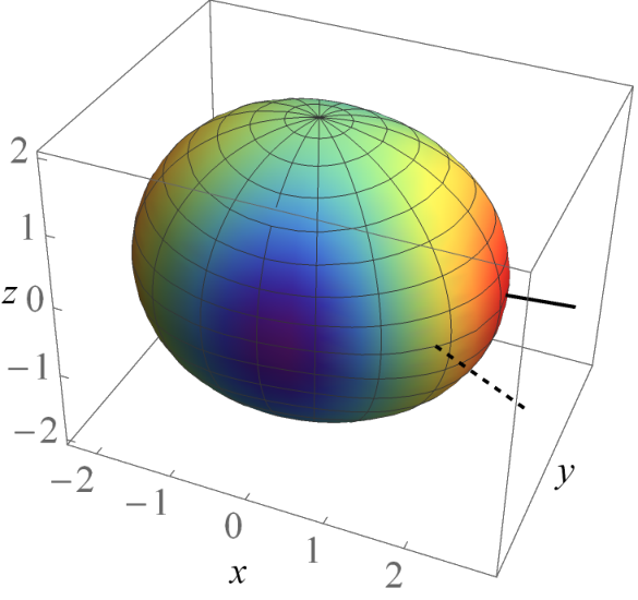
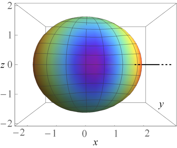
As a final element of our discussion, we present a visualization of the horizon. Unlike the rest of the paper, this section is necessarily restricted to linear perturbations. The reason is simple: the visualization requires modes with , and no second-order data is yet available for these modes. Because of this restriction, our presentation here largely reproduces earlier literature. However, we highlight an aspect of the visualization that was omitted in earlier descriptions: the motion of the black hole. We also point out that features described as teleological in the literature cannot have a truly teleological origin, and we offer an alternative explanation for the behavior.
In this section we also depart from our treatment in other sections in that we specifically focus on behavior on the orbital timescale rather than trying to maintain accuracy on both the orbital and radiation-reaction timescale. This means that we may make the replacement , as in Eq. (295), which is consistent at first order in on the orbital time scale.
VII.3.1 Motion of the black hole
We first review the visualization method outlined in Refs. 84; 56 (following earlier work in Refs. 35; 36). Since the horizon’s coordinate radius is inherently gauge dependent, and actually identical to the background horizon’s radius in a horizon-locking gauge, the method instead depicts the shape of the horizon based on its intrinsic curvature. To do so, one embeds the horizon into 3-dimensional Euclidean space.
The embedding is found by constructing a closed 2-surface in Euclidean space that has the same intrinsic curvature as the horizon. In Cartesian coordinates , at a given value of , such a surface can be parametrized as
| (307) |
where is the usual radial unit vector, which satisfies . We write the radius of the surface as
| (308) |
and we expand the small correction as
| (309) |
The metric on the surface, induced from the Euclidean metric , is
| (310) |
where we have discarded the term of order . Noting that this metric is of the form (47), we can read off its scalar curvature from Eqs. (89) and (95), with and . This yields
| (311) |
where, recall, , and we again omit terms.
Finally, equating the curvature to the intrinsic curvature (89) of the horizon, we obtain the radial profile through linear order:
| (312) |
is calculated from the coefficients and in the expansion (299), evaluated at , using Eq. (95) with Eqs. (59) and (301). Since the scalar curvature is invariant at first order, Eq. (312) then provides an invariant representation of the horizon’s radial profile.
There are several things to note about this construction. First, the metric (310) is manifestly identical to the intrinsic metric on for a particular choice of gauge, as described in Sec. VI.2.3. In that section we imposed the gauge choice only on the slowly varying part of the intrinsic metric, but it can be imposed on the oscillatory part as well. The second thing to note is that because the two horizons are identical at linear order, this visualization represents the apparent horizon as well as the event horizon. Finally, we note that Eq. (312) has a significant shortcoming as a representation of the horizon. While it provides a meaningful depiction of the horizon’s shape, it does not contain any information about the horizon’s location. In a binary system, both bodies orbit around the system’s center of mass, and a faithful representation of the black hole horizon should encode this motion.
The information about the horizon’s location is encoded in the term in the metric perturbation. Since the construction leading to Eq. (312) only requires that the embedded surface has the same intrinsic geometry as the horizon, and since gets zero contribution from modes, we can in principle add any arbitrary term to . In previous analyses, the dipole term was simply set to zero, as we have implicitly done in Eq. (312). This is a sensible choice if we are only concerned with the horizon’s shape, but not if we are concerned with its location. To construct a more faithful representation of the black hole horizon, we should instead replace the embedding (307) with
| (313) |
In this representation, at each moment , the surface is drawn around the black hole’s “center” . We must now find a meaningful way of measuring this center.
To see how relates to an mode, assume . Then the radial location of a point on the surface is
| (314) |
The quantity is a pure dipole. If we define a new radial profile and expand it as , then corresponds to the coefficients:
| (315) |
In these expressions we absorb the dependence into the coefficients. Note that although we have this one-to-one relationship, the embedding (313) should be used rather than ; in Eq. (313), the term represents a uniform translation, shifting the center of the black hole without altering its shape, while in it does visibly alter the shape.
We now require a meaningful to use in Eq. (315). One option would be to simply use the mode of the coordinate profile (301) in the Lorenz gauge. While the coordinate profile is a gauge-dependent quantity, there is good reason to think the Lorenz-gauge profile contains a meaningful dipole mode. As explained in Ref. 24, if the coordinate system is centered on the moving black hole, then the coordinates are noninertial, causing the metric at large to grow rather than decay. The transformation from such a gauge to the Lorenz gauge eliminates this feature, and in the Lorenz gauge one can identify the system’s center of mass with the coordinate origin (of course keeping in mind that this is only an effective identification because the coordinate origin is deep inside the black hole and not a well-defined curve in the true spacetime manifold).
Unfortunately, the Lorenz-gauge dipole leads to counterintuitive behavior that does not scale correctly in the Newtonian limit. In Newtonian theory, if the black hole moves on a trajectory and the particle on a trajectory , then the system’s center of mass is , and if the center of mass is at the coordinates’ origin, then . The magnitude of the black hole’s displacement should then be , growing linearly with the particle’s orbital radius . In fact, the Lorenz-gauge dipole does encode such linear growth 55, and we can even observe the growth in the metric perturbation on the horizon. However, the radial profile (301) only depends on a specific piece of this perturbation, , and we find that this decays as at large .55 5 The alternative formula (116) does depend on other pieces of the dipole perturbation, but those pieces are found to precisely cancel. We then arrive at a puzzling conclusion. If we follow an inspiral backward in time, such that the particle spirals outward toward greater radii, then far from the system, in the wave zone, the metric appears to behave as if the coordinates are centered on the center of mass, with the black hole also spiralling outward. But if we make a local measurement of the horizon’s location, we find that while the particle spirals outward, the black hole spirals inward, eventually settling precisely at the coordinate origin.
As an alternative to the Lorenz-gauge measure of the black hole’s center, we can follow the idea that Eq. (310) is a gauge-fixed version of the horizon’s intrinsic metric . After eliminating via a gauge choice, we have . We can then put this in the form (310) by performing a uniform translation, by an amount , to eliminate the dipole mode from . This transformation would make the induced metric perfectly round up to contributions, as it should be if the coordinates are centered on the center of the black hole. We can then undo the translation, but now treating it exactly rather than perturbatively, to obtain the displaced surface (313). In that expression, is given by Eq. (315) with . Explicitly, appealing to Eq. (59) for , we see that
| (316) |
where is given by Eq. (301).
We use this definition of black hole’s center in Figs. 2–3, which display the horizon surface (313) in the – plane at several values of and for two values of . In these plots, we see two effects: the horizon is tidally distorted by the orbiting companion, and it follows a counterclockwise orbit around the center of mass. (We have artificially multiplied modes of by a factor of 200 to make the tidal distortion clearly visible. Other parameters are described in the captions.)
Unfortunately, this definition of the black hole’s position does not exhibit the expected Newtonian behavior. We find numerically that tends to at large rather than to . The linear scaling with is correct, and it is quite unlike the behavior of the Lorenz-gauge coordinate position. But there is a confounding factor-of-2 disagreement. This suggests that a different definition of is required. We leave investigation of this issue to future work.
VII.3.2 Horizon teleology
Like the black hole, the companion follows a counterclockwise orbit, with a trajectory , such that at advanced time it is at a position
| (317) |
where is the tortoise coordinate at the particle’s location. In each plot, the dotted line points toward this position. The dashed line points toward the location of greatest tidal distortion of the horizon---the tidal bulge. As we can see from the plots, the tidal bulge consistently leads the companion’s orbit by a constant angle, seeming to point toward the companion’s future location.66 6 Note that the displacement of the black hole from the center of mass creates an correction to the angle between the two lines.
This lead angle has been discussed many times in the past 36; 28; 84; 56. It markedly contrasts with the behavior of a fluid body. In Newtonian physics, the tidal bulge of an inviscid fluid body points toward the companion’s instantaneous position. If the fluid is viscous, then the tidal bulge lags behind the companion’s orbit. In relativistic physics, the tidal bulge will also lag due to retardation. In no case does the fluid body’s bulge lead the companion’s orbit. Previous literature has offered the explanation that the tidal lead is due to the teleological nature of the event horizon: the horizon effectively anticipates the companion’s future location. More mathematically, Eq. (143) tells us that the horizon’s deformation leads the metric perturbation by a time of order .
However, such an explanation cannot be wholly correct. At linear order, the event horizon is indistinguishable from the apparent horizon: their radial profiles (143) (with ) and (116) are identical. Therefore the event horizon’s location on a slice of constant advanced time is completely determined by information on that slice. This rules out a truly teleological explanation, but it also suggests a nonteleological one. An apparent horizon is not pulled toward the orbiting companion; it is repelled by it. This is because the companion pulls light rays toward itself and hence away from the black hole, helping them to escape. Therefore the tidal bulge of the horizon cannot be interpreted in the same way as the tidal bulge of a fluid body. The bulge of a fluid body is created by the companion pulling the fluid toward itself, while the companion’s pull on light rays has precisely the opposite effect on the black hole’s horizon. Rather than thinking of the bulge leading the orbit, we can think of the depression lagging the orbit due to retardation.
Of course, this only describes the behavior of the side of the horizon nearest the companion. But we can also explain the behaviour of the other sides. The bulge is created because on the bulging sides of the horizon, light rays pulled toward the companion fall into the hole, and the orientation of this effect again lags the orbit due to retardation. There is a less obvious reason why the far side of the horizon is depressed. Naively, one would expect that since the companion pulls light rays toward itself, it will pull them into the black hole if they are on the far side of the hole. This would suggest that the horizon should bulge outward on the far side, rather than being depressed. However, it is depressed there for the same reason that a fluid body bulges there: the companion’s pull is weaker on the far side than at the black hole’s “center”, meaning the companion pulls the black hole’s center toward itself more than it pulls light rays into the black hole.
Although these simplistic descriptions ignore the complexity of field propagation in the strong gravity of the black hole, it is clear that since the horizon is an apparent horizon, there must be a nonteleological explanation of its shape and orientation. This conclusion is reinforced by the fact that similar behavior has been observed in the apparent horizon in full numerical relativity 77.
One might wonder (a) how this is reconciled with the teleological solution (143), and (b) whether the lead angle is fundamentally a teleological effect that only becomes effectively causal as a consequence of the temporal localization of the event horizon in a binary. We believe both questions are answered by the fact that the shape we have plotted is an apparent horizon regardless of whether or not it is the event horizon: the radial profile of the apparent horizon, (116), encodes the lead angle. This tells us that the tidal deformation at time is determined solely by the behavior of null vectors at time . In the case that the event horizon becomes temporally localized, reducing the teleological solution (143) to the localized solution (159), then it too only depends on the behavior of null vectors at time ; the localized solution only encodes the teleological nature of (143) in the weak sense of encoding the tangent vector to a curve at time (as opposed to only encoding the location of the curve at that time). The “lead time” is only teleological in that same weak sense. It is simply a statement about null tangent vectors, rather than a statement about the far future of null curves.
Yet the teleological solution (143) does impose boundary conditions in the future. What is their relevance? They only serve to rule out exponentially growing solutions, which would describe null curves that escape to infinity.77 7 Note also that Eq. (159) is the unique solution to Eq. (135) if we assume a two-timescale ansatz. The future boundary conditions therefore only ensure that the null curves are marginally trapped. In other words, they ensure that the event horizon remains close to the apparent horizon. Rather than inferring that the apparent horizon exhibits the event horizon’s teleological behavior, we can infer that the event horizon, by hewing close to the apparent horizon, exhibits the apparent horizon’s nonteleological behavior.
We also stress that the identification of the two horizons does not depend on the localization: at linear perturbative order, the event horizon is an apparent horizon under fairly general conditions. In the context of a binary, the linear-order identification only breaks down as the companion enters into its plunge. In those final moments, teleological effects do arise at linear order, as additional null rays join the event horizon in anticipation of the companion’s entry into the black hole 34; 27; 45; 26.
To more starkly illustrate that difference between the teleological and the nonteleological, we can consider a thought experiment in which the companion orbits the black hole while a pulse of null radiation approaches on a radial trajectory. Suppose the pulse is timed such that it strikes the companion and sends it into either a plunge or an escape trajectory. The pulse approaches on a surface . For all , the pulse is out of causal contact with the black hole, and the apparent horizon behaves just as we have illustrated it. But the event horizon anticipates the pulse, and additional generators begin to join it. At a time , this teleological effect becomes significant. If the pulse ultimately knocks the companion into the black hole, then at , the event horizon must already be significantly reaching out to meet the companion’s plunge. If instead the pulse sends the companion into an escape trajectory, then at the event horizon must already be adjusting itself in a very different way. Yet at the apparent horizon is identical in both cases. Unaffected by the future events, it continues to exhibit the same tidally deformed shape with the same lead angle.
VIII Conclusion
In this paper, motivated by the work that was necessary in Ref. 64, we have focused on a few features of perturbed horizons: their location and surface area, the quasilocal mass they contain, and their scalar curvature. We have primarily highlighted the degree to which the apparent and event horizon differ beginning at second perturbative order. In particular, we have established the relationships (274), (278), (282), and (283) between the horizons’ radii, intrinsic metrics, scalar curvatures, and surface areas, along with the equality (286) of their Hawking masses. Although we have not discussed the Hawking-Hayward mass 42, an immediate corollary of our results is that the two horizons also have equal values of through order .
Our results have illuminated several important, but subtle issues that arise in the study of perturbed black holes. First, we have highlighted the fact that the apparent and event horizons are identical at first perturbative order (except in certain cases such as shortly before merger in a binary). This was already known, as it is a simple consequence of the event horizon’s expansion scalar vanishing at linear order, but to our knowledge it has not been emphasized in the literature. Because the event horizon is indistinguishable from an apparent horizon at linear order, one must be cautious in ascribing any teleological interpretation to its behavior at this order. In Sec. VII.3 we have explained how even seemingly teleological behavior such as the “tidal lead” in a binary is actually nonteleological in origin.
Along the same lines, in Sec. V.3 we have shown how, in a small-mass-ratio binary, the event horizon of the central black hole is effectively localized in time at all perturbative orders. This result establishes that in the small-mass-ratio context, teleological effects are negligible even beyond linear order.
Another important conclusion follows from our result that the apparent and event horizons have identical Hawking masses through second order. The Hawking mass of the apparent horizon grows monotonically, obeying a physically intuitive “flux-balance” law 9, which implies that the mass grows at the rate that energy crosses the horizon. Our result therefore shows that the Hawking mass of the event horizon obeys the same flux-balance law at least through second order. Besides its intrinsic interest, this may be useful in deriving and interpreting second-order balance laws for small-mass-ratio inspirals, which would relate the evolution of the companion’s orbit to (i) the evolution of the central black hole, and (ii) the gravitational waves emitted to infinity.
All our results have been obtained in two formulations: in a form that does not specify a choice of gauge, and in a gauge-fixed form. In either case, the metric-perturbation inputs can be calculated in any gauge. If one uses the unfixed formulas, one’s choice of gauge will influence one’s results for the horizon area and scalar curvature, for example. That may or may not be advantageous depending on context; one might wish to use a gauge condition corresponding to a specific choice of horizon foliation, for example. On the other hand, the gauge-fixed formulation provides invariant results carrying a specific geometric interpretation.
From this starting point, there are many obvious follow-ons that we leave to future work. First, one might derive perturbative formulas for the black hole’s spin and higher multipole moments.
Second, our results have revealed a puzzling discrepancy between the location of the horizon and the expected Newtonian limit. To better characterize the black hole’s orbit around the system’s center of mass, one might derive a perturbative formula for an invariant linear momentum such as the Hawking momentum 78 or an analogous orbital angular momentum.
Third, in a dynamically evolving spacetime with a two-timescale character, can we meaningfully identify an average horizon that only evolves on the slow timescale, and is it precisely a Kerr horizon with slowly evolving mass and spin, or does it contain higher moments that deviate from Kerr? Such a study might draw on the framework of slowly evolving horizons in Ref. 16.
To characterize this average horizon, a critical step would be obtaining flux-balance equations governing the evolution of the averaged mass, spin, and higher moments. This would involve higher-order extensions of standard relations for the black hole’s mass and spin evolution in terms of the shear of the horizon generators 61, as well as equations for the higher moments that describe black hole memory effects 40; 73.
Finally, an important goal will be to numerically compute these second-order effects on the horizon in realistic binary scenarios. That programme of research was initiated in the calculation of the apparent horizon’s irreducible mass in Ref. 64, and more such calculations will soon be possible. Since the event horizon begins to differ from the apparent horizon at second order, these calculations may also allow us to identify genuine teleological effects during an inspiral.
Acknowledgements.
We are grateful to Niels Warburton and Barry Wardell, who kindly provided input data used within this paper, and to Eric Poisson for a sanity check and a helpful discussion. This work makes use of the Black Hole Perturbation Toolkit 1. RB thanks Stefano Ansoldi for introducing him to these topics. AP thanks Aaron Zimmerman for suggesting an analysis of the apparent horizon and for additional helpful discussions in the early stages of this work; Jonathan Thornburg for pointing out the exponential suppression of teleological effects on the event horizon; Leor Barack for helpful conversations and for independently checking some of our first-order results. ZS additionally thanks Tim Dietrich for his interest in this work and comments on an earlier version of the manuscript. RB additionally thanks the University of Trieste for the International Mobility Scholarship granted, and in turn the University of Southampton for the welcoming hospitality. AP also gratefully acknowledges the support of a Royal Society University Research Fellowship. AP’s early work in this paper was supported by the European Research Council under the European Union’s Seventh Framework Programme (FP7/2007-2013)/ERC Grant No. 304978.Appendix A Perturbative formulas for curvature tensors
In this appendix we review the derivation of perturbed curvature tensors through second order. Because we use these formulas for the curvature of the horizon, not solely for the Einstein equations, we allow the background metric to have nonvanishing Ricci curvature. Unlike in the body of the paper, here we use the inverse of the background metric to raise indices.
The derivation follows standard methods in Ref. 87, for example. We consider a generic metric of the form . The Christoffel symbols associated with and those associated with are related by
| (318) |
where
| (319) |
and a semicolon denotes covariant differentiation compatible with . In terms of this tensor, the Riemann tensors of the two metrics are related by
| (320) |
The Ricci tensors are therefore related by
| (321) |
We now expand the Ricci tensor in powers of using
| (322) |
The result is
| (323) |
where
| (324) |
and
| (325) |
where a denotes trace reversal, as in .
The perturbations of the Ricci scalar are straightforwardly deduced from those of the Ricci tensor. We have
| (326) |
with
| (327) | ||||
| (328) |
Explicitly,
| (329) |
and
| (330) |
Appendix B Coupling of spherical harmonics
In various places in the body of the paper, we must decompose products of angular functions into scalar spherical harmonics. That is, for a function , we require
| (331) |
Each of the angular functions in the integrand is itself expressed as a sum of harmonics, leading to integrals with the schematic form
| (332) |
where and are constructed from through linear operations involving , , , and .
To evaluate such derivatives, we express the integrand in terms of spin-weighted spherical harmonics, which are constructed from a complex basis on . We define
| (333) |
in spherical coordinates ; the basis is then . These basis vectors have the useful properties
| (334) | ||||
| (335) | ||||
| (336) | ||||
| (337) | ||||
| (338) | ||||
| (339) |
Our definition of differs by a factor of relative to that of Ref. 53, and it is normalized on the unit sphere rather than a sphere of radius . In terms of , we define derivative operators and that act on a scalar of spin-weight as
| (340) | ||||
| (341) |
Our definitions here differ by an overall minus sign relative to those of Ref. 53. A quantity has spin-weight if it transforms as under the complex rotation . raises the spin weight by 1, while lowers it by 1.
The spherical harmonics of spin-weight are
| (342) |
where
| (343) |
The integral of three spin-weighted harmonics is
| (344) |
In the case that , the coupling constants are given by
| (345) |
where the arrays are symbols. These symbols inherit symmetries from the symbols, specifically
| (346) | ||||
| (347) | ||||
| (348) |
For and , they have the special value
| (349) |
We evaluate all integrals of the form (332) by expressing the integrand as a sum of terms of the form (344). This is straightforwardly accomplished by applying the identities (334)–(339) and the definitions (14)–(17). For example, together with Eqs. (340) and (341) leads to
| (350) |
The specific integrals involved in calculating are found to be
| (351) | ||||
| (352) | ||||
| (353) | ||||
| (354) |
where , ,
| (355) |
In the calculation of , third angular derivatives of arise. These are treated in the same way, with higher-order versions of Eq. (350) containing spin weights up to .
Appendix C Second-order expressions
In this appendix we compile results for various second-order quantities.
The functions of appearing in the mode decomposition (96) of the second-order scalar curvature are
| (356a) | ||||
| (356b) | ||||
| (356c) | ||||
| (356d) | ||||
where is defined in Eq. (343), , , and and are defined in Eq. (355). In these expressions we have introduced the compact notation , , and so on, along with the combinations , and (suppressing labels).
The second-order term appearing in the expansion scalar (113) is
| (357) |
The functions appearing in the mode decomposition (117) of are given by
| (358a) | ||||
| (358b) | ||||
| (358c) | ||||
where , and we define , , and so on. The combinations , , , and are defined in terms of and following the notation described below Eq. (356). In the gauge-fixed form of Sec. VI, these coefficients become
| (359a) | ||||
| (359b) | ||||
The term in the second-order correction to the apparent horizon’s radius, (118), is
| (360) |
Finally, the quantities and appearing in Eq. (305) are given by
| (361) | ||||
| (362) |
All quantities here are evaluated at . When acting on a nonconjugated quantity, ; on a conjugated quantity, . The harmonic coefficients of are given in Sec. VI, with the mode-number replacement :
The quantity has tensor-harmonic coefficients , , , and
| (363) | ||||
| (364) | ||||
| (365) | ||||
| (366) | ||||
| (367) | ||||
| (368) |
where, again, all quantities are evaluated at . and can be read off of Eqs. (201) and (202).
References
- [1] Note: The Black Hole Perturbation Toolkit is available at https://bhptoolkit.org/toolkit.html Cited by: §VIII.
- Charge Definition in Nonabelian Gauge Theories. Phys. Lett. B 116, pp. 259–263. External Links: Document Cited by: §IV.3.
- GWTC-2: Compact Binary Coalescences Observed by LIGO and Virgo During the First Half of the Third Observing Run. Phys. Rev. X 11, pp. 021053. External Links: 2010.14527, Document Cited by: §I.1.
- Frequency-domain algorithm for the Lorenz-gauge gravitational self-force. Phys. Rev. D 88 (10), pp. 104009. External Links: 1308.5223, Document Cited by: §VII.1.
- First M87 Event Horizon Telescope Results. I. The Shadow of the Supermassive Black Hole. Astrophys. J. 875 (1), pp. L1. External Links: 1906.11238, Document Cited by: §I.1.
- Research Update on Extreme-Mass-Ratio Inspirals. J. Phys. Conf. Ser. 610 (1), pp. 012002. External Links: 1410.0958, Document Cited by: §I.1.
- The gravitational capture of compact objects by massive black holes. External Links: 2011.03059 Cited by: §I.1.
- Some uniqueness results for dynamical horizons. Adv. Theor. Math. Phys. 9 (1), pp. 1–30. External Links: gr-qc/0503109, Document Cited by: §I.2.
- Isolated and dynamical horizons and their applications. Living Rev. Rel. 7, pp. 10. External Links: gr-qc/0407042, Document Cited by: §I.2, §IV.1, §VIII.
- Late time decay of gravitational and electromagnetic perturbations along the event horizon. Phys. Rev. D 60, pp. 124005. External Links: gr-qc/9907085, Document Cited by: §V.3.
- Self-force and radiation reaction in general relativity. Rept. Prog. Phys. 82 (1), pp. 016904. External Links: 1805.10385, Document Cited by: §I.1.
- Prospects for Fundamental Physics with LISA. Gen. Rel. Grav. 52 (8), pp. 81. External Links: 2001.09793, Document Cited by: §I.1.
- Quasinormal modes of black holes and black branes. Class. Quant. Grav. 26, pp. 163001. External Links: 0905.2975, Document Cited by: §V.3.
- Spectroscopy of Kerr black holes with Earth- and space-based interferometers. Phys. Rev. Lett. 117 (10), pp. 101102. External Links: 1605.09286, Document Cited by: §I.1.
- Parallel adaptive event horizon finder for numerical relativity. Phys. Rev. D 94 (6), pp. 064008. External Links: 1606.00437, Document Cited by: §I.2.
- The First law for slowly evolving horizons. Phys. Rev. Lett. 92, pp. 011102. External Links: gr-qc/0307087, Document Cited by: §VIII.
- Black hole boundaries. Can. J. Phys. 83, pp. 1073–1099. External Links: gr-qc/0508107, Document Cited by: §I.2.
- A Complete gauge-invariant formalism for arbitrary second-order perturbations of a Schwarzschild black hole. Phys. Rev. D 80, pp. 024021. External Links: 0903.1134, Document Cited by: §II.1.
- Perturbations of space-time: Gauge transformations and gauge invariance at second order and beyond. Class.Quant.Grav. 14, pp. 2585–2606. External Links: Document, gr-qc/9609040 Cited by: §II.1.
- Second order gauge invariant gravitational perturbations of a Kerr black hole. Phys. Rev. D 59, pp. 124022. External Links: gr-qc/9811019, Document Cited by: §I.1.
- Testing the nature of dark compact objects: a status report. Living Rev. Rel. 22 (1), pp. 4. External Links: 1904.05363, Document Cited by: §I.1.
- Reversible and irreversible transformations in black-hole physics. Phys. Rev. Lett. 25, pp. 1596. Cited by: §III.3.
- Revisiting Event Horizon Finders. Class. Quant. Grav. 26, pp. 035005. External Links: 0809.2628, Document Cited by: §I.2, §I.2.
- Low multipole contributions to the gravitational selfforce. Phys. Rev. D 69, pp. 084019. External Links: gr-qc/0312010, Document Cited by: §VII.3.1.
- Self-force via -mode regularization and 2+1D evolution: III. Gravitational field on Schwarzschild spacetime. Phys. Rev. D 87, pp. 084066. External Links: 1211.4586, Document Cited by: §IV.3.
- Black hole fusion in the extreme mass ratio limit. Phys. Rev. D 97 (4), pp. 044004. External Links: 1708.08868, Document Cited by: §I.2, §I.3, §V.3, §VII.3.2.
- Exact Event Horizon of a Black Hole Merger. Class. Quant. Grav. 33 (15), pp. 155003. External Links: 1603.00712, Document Cited by: §I.2, §I.3, §V.3, §VII.3.2.
- Tidal coupling of a Schwarzschild black hole and circularly orbiting moon. Phys. Rev. D 72, pp. 124016. External Links: gr-qc/0505156, Document Cited by: §VII.3.2.
- An Efficient Numerical Method for Computing Gravitational Waves Induced by a Particle Moving on Eccentric Inclined Orbits around a Kerr Black Hole. Prog. Theor. Phys. 121, pp. 843–874. External Links: 0904.3810, Document Cited by: §VII.2.
- Testing General Relativity with Low-Frequency, Space-Based Gravitational-Wave Detectors. Living Rev. Rel. 16, pp. 7. External Links: 1212.5575, Document Cited by: §I.1.
- New theoretical approaches to black holes. New Astron. Rev. 51, pp. 791–798. External Links: 0803.2944, Document Cited by: §I.2.
- The shape of the black hole photon ring: A precise test of strong-field general relativity. Phys. Rev. D 102 (12), pp. 124004. External Links: 2008.03879, Document Cited by: §I.1.
- Teukolsky formalism for nonlinear kerr perturbations. Classical and Quantum Gravity 37 (7), pp. 075001. External Links: ISSN 1361-6382, Link, Document Cited by: §I.1.
- Event Horizon Deformations in Extreme Mass-Ratio Black Hole Mergers. Phys. Rev. D 84, pp. 124015. External Links: 1007.5387, Document Cited by: §I.2, §I.3, §V.3, §VII.3.2.
- Tidal Friction in Slowly Rotating Black Holes. Phys. Rev. D 8, pp. 1010–1024. External Links: Document Cited by: §I.2, §VII.3.1.
- Tidal shapes and shifts on rotating black holes. Phys. Rev. D 9, pp. 2749–2759. External Links: Document Cited by: §I.2, §VII.3.1, §VII.3.2.
- The Large Scale Structure of Space-Time. Cambridge Monographs on Mathematical Physics, Cambridge University Press. External Links: Document, ISBN 978-0-521-20016-5, 978-0-521-09906-6, 978-0-511-82630-6, 978-0-521-09906-6 Cited by: §I.2.
- Energy and angular momentum flow into a black hole. Commun. Math. Phys. 27, pp. 283–290. External Links: Document Cited by: §I.2.
- The event horizon. In Black Holes, C. DeWitt and B. S. DeWitt (Eds.), pp. 1–55. Cited by: §I.2.
- Soft Hair on Black Holes. Phys. Rev. Lett. 116 (23), pp. 231301. External Links: 1601.00921, Document Cited by: §I.3, §VIII.
- General laws of black hole dynamics. Phys. Rev. D 49, pp. 6467–6474. External Links: gr-qc/9303006 Cited by: §I.2.
- Quasilocal gravitational energy. Phys. Rev. D 49, pp. 831–839. External Links: gr-qc/9303030, Document Cited by: §III.3, §VIII.
- Dynamics of black holes. External Links: 0810.0923 Cited by: §I.2.
- Two timescale analysis of extreme mass ratio inspirals in Kerr. I. Orbital Motion. Phys. Rev. D 78, pp. 064028. External Links: 0805.3337, Document Cited by: §II.4.
- Deformation of horizons during a merger. Class. Quant. Grav. 35 (1), pp. 015013. External Links: 1705.01510, Document Cited by: §I.2, §I.3, §V.3, §VII.3.2.
- Mass and Angular Momentum in General Relativity. Fundam. Theor. Phys. 162, pp. 87–124. External Links: 1001.5429, Document Cited by: §III.3.
- Multiple scale and singular perturbation methods. Springer, New York. Cited by: §II.4.
- Fundamental properties and applications of quasi-local black hole horizons. Class. Quant. Grav. 25, pp. 114005. External Links: 0712.1575, Document Cited by: §I.2.
- Second Order Perturbations of Kerr Black Holes: Reconstruction of the Metric. Phys. Rev. D 103 (10), pp. 104017. External Links: 2008.11770, Document Cited by: §I.1.
- Science Case for the Einstein Telescope. JCAP 03, pp. 050. External Links: 1912.02622, Document Cited by: §I.1.
- Gravitational perturbations of the Schwarzschild spacetime: A Practical covariant and gauge-invariant formalism. Phys. Rev. D 71, pp. 104003. External Links: gr-qc/0502028, Document Cited by: §II.1, §II.2, §II.2, §II.3.
- Two-timescale evolution of extreme-mass-ratio inspirals: waveform generation scheme for quasicircular orbits in Schwarzschild spacetime. Phys. Rev. D 103 (6), pp. 064048. External Links: 2006.11263, Document Cited by: §II.4, §IV.3, §VII.1, §VII.1.
- Note on the Bondi-Metzner-Sachs group. J. Math. Phys. 7, pp. 863. Cited by: Appendix B, Appendix B.
- The Transition from inspiral to plunge for a compact body in a circular equatorial orbit around a massive, spinning black hole. Phys. Rev. D 62, pp. 124022. External Links: gr-qc/0003032, Document Cited by: §II.4, §V.3, §VII.1.
- Harmonic gauge dipole metric perturbations for weak field circular orbits in Schwarzschild space-time. Phys. Rev. D 70, pp. 124027. External Links: gr-qc/0312013, Document Cited by: §VII.3.1.
- Strong-field tidal distortions of rotating black holes: Formalism and results for circular, equatorial orbits. Phys. Rev. D 90 (12), pp. 124039. Note: [Erratum: Phys.Rev.D 91, 109901 (2015)] External Links: 1407.6983, Document Cited by: §I.2, §VII.3.1, §VII.3.2.
- Strong-field tidal distortions of rotating black holes: II. Horizon dynamics from eccentric and inclined orbits. Phys. Rev. D 94 (4), pp. 044057. External Links: 1505.03809, Document Cited by: §I.2.
- Strong-field tidal distortions of rotating black holes. III. Embeddings in hyperbolic three-space. Phys. Rev. D 96 (6), pp. 064030. External Links: 1704.05471, Document Cited by: §I.2.
- Extraction of rotational energy from a black hole. Nature Physical Science 229 (6), pp. 177–179. External Links: Document Cited by: §III.3.
- A relativist’s toolkit: the mathematics of black-hole mechanics. Cambridge University Press. Cited by: §IV.
- Absorption of mass and angular momentum by a black hole: Time-domain formalisms for gravitational perturbations, and the small-hole / slow-motion approximation. Phys. Rev. D 70, pp. 084044. External Links: Document, gr-qc/0407050 Cited by: §I.2, §I.2, §V.3, §V.4, §V, §VI.3, §VIII.
- Horizons in a binary black hole merger I: Geometry and area increase. External Links: 2006.03939 Cited by: §I.2.
- Horizons in a binary black hole merger II: Fluxes, multipole moments and stability. External Links: 2006.03940 Cited by: §I.2.
- Second-Order Self-Force Calculation of Gravitational Binding Energy in Compact Binaries. Phys. Rev. Lett. 124 (2), pp. 021101. External Links: 1908.07419, Document Cited by: §I.1, §I.2, §VII.1, §VII.1, §VII.2, §VII.2, §VII.2, §VII, §VIII, §VIII.
- Black hole perturbation theory and gravitational self-force. External Links: 2101.04592 Cited by: §I.1, §II.1, §II.4, §II.4, §II.4, footnote 1.
- Singular perturbation techniques in the gravitational self-force problem. Phys. Rev. D 81, pp. 124009. External Links: 1003.3954, Document Cited by: §II.4.
- Gauge and motion in perturbation theory. Phys. Rev. D 92 (4), pp. 044021. External Links: 1506.02894, Document Cited by: §II.1.
- News from horizons in binary black hole mergers. Phys. Rev. Lett. 125 (12), pp. 121101. External Links: 2003.06215, Document Cited by: §I.3.
- A light-cone gauge for black-hole perturbation theory. Phys. Rev. D 74, pp. 064010. External Links: gr-qc/0606094, Document Cited by: §VI.2.2.
- Membrane Viewpoint on Black Holes: Properties and Evolution of the Stretched Horizon. Phys. Rev. D 33, pp. 915–941. External Links: Document Cited by: §I.2.
- Nonspherical perturbations of relativistic gravitational collapse. 1. Scalar and gravitational perturbations. Phys. Rev. D 5, pp. 2419–2438. External Links: Document Cited by: §V.3.
- Gravitational Test Beyond the First Post-Newtonian Order with the Shadow of the M87 Black Hole. Phys. Rev. Lett. 125 (14), pp. 141104. External Links: 2010.01055, Document Cited by: §I.1.
- Black Hole Memory. Phys. Rev. D 101 (12), pp. 124010. External Links: 1912.12806, Document Cited by: §I.3, §VIII.
- Numerical computation of second order vacuum perturbations of Kerr black holes. Phys. Rev. D 103, pp. 104018. External Links: 2010.00162, Document Cited by: §I.1.
- Introduction to dynamical horizons in numerical relativity. Phys. Rev. D 74, pp. 024028. External Links: gr-qc/0604015, Document Cited by: §I.2, §I.2.
- Location of the last stable orbit in Kerr spacetime. Phys. Rev. D 101 (6), pp. 064007. External Links: 1912.07609, Document Cited by: §V.3.
- [77] Note: private communication Cited by: §VII.3.2.
- Quasi-Local Energy-Momentum and Angular Momentum in General Relativity. Living Rev. Rel. 12, pp. 4. External Links: Document Cited by: §VIII.
- Small mass plunging into a Kerr black hole: Anatomy of the inspiral-merger-ringdown waveforms. Phys. Rev. D 90 (8), pp. 084025. External Links: 1404.1819, Document Cited by: §V.3.
- Perturbations of a rotating black hole. III - Interaction of the hole with gravitational and electromagnet ic radiation. Astrophys. J. 193, pp. 443–461. External Links: Document Cited by: §I.2.
- A Fast apparent horizon finder for three-dimensional Cartesian grids in numerical relativity. Class. Quant. Grav. 21, pp. 743–766. External Links: gr-qc/0306056, Document Cited by: §I.2.
- Event and apparent horizon finders for 3+1 numerical relativity. Living Rev. Rel. 10, pp. 3. External Links: gr-qc/0512169 Cited by: §I.2.
- Resonantly enhanced kicks from equatorial small mass-ratio inspirals. Phys. Rev. D 90 (4), pp. 044027. External Links: 1406.2594, Document Cited by: footnote 1.
- Intrinsic and extrinsic geometries of a tidally deformed black hole. Class. Quant. Grav. 28, pp. 175006. External Links: 1106.0510, Document Cited by: §I.2, §I.2, §II.2, §III.4, §V.3, §V.4, §V, §VI.2.1, §VI.2.2, §VI, §VII.3.1, §VII.3.2.
- EHT tests of the strong-field regime of General Relativity. External Links: 2011.06812 Cited by: §I.1.
- Trapped surfaces in the Schwarzschild geometry and cosmic censorship. Phys. Rev. D 44, pp. 3719–3722. External Links: Document Cited by: §I.2.
- The University of Chicago Press, Chicago and London. Cited by: Appendix A.
- Gravitational waveforms for compact binaries from second-order self-force theory. External Links: 2112.12265 Cited by: §VII.2.