跳到论文正文
W Papers独立论文阅读器 arXiv:2109.09335 论文正文 计算阅读时间 · 0%
引用这篇论文根据当前论文元数据生成,正式投稿前建议核对。


License: CC BY-NC-ND 4.0
arXiv:2109.09335v1 [cs.IT] 20 Sep 2021

Spectral and Energy Efficiency of Multicell Massive MIMO With Variable-Resolution ADCs Over Correlated Rayleigh Fading ChannelsThanks: This work was supported in part by National Natural Science Foundation of China (NSFC) under Grants 62101370, 61871070, 91938202, and 61831004, in part by Sichuan Science and Technology Program under Grant 2021YFG0013. (Corresponding author: Youzhi Xiong.)Thanks: Youzhi Xiong, Sanshan Sun, and Li Liu are with College of Physics and Electronic Engineering, Sichuan Normal University, Chengdu, 610068, China. (e-mail: yzxiong@sicnu.edu.cn; sanshansun@hotmail.com; liuli@sicnu.edu.cn). Ning Wei and Zhongpei Zhang are with National Key Laboratory of Science and Technology on Communications, University of Electronic Science and Technology of China, Chengdu, 611731, China. (e-mail: wn@uestc.edu.cn; zhangzp@uestc.edu.cn)

Youzhi Xiong    Sanshan Sun    Member IEEE    Ning Wei    Member IEEE Affiliation: Li Liu, and Zhongpei Zhang, Member IEEE
Abstract

This paper analyzes the performance of multicell massive multiple-input and multiple-output (MIMO) systems with variable-resolution analog-to-digital converters (ADCs). In such an architecture, each ADC uses arbitrary quantization resolution to save power and hardware cost. Along this direction, we first introduce a quantization-aware channel estimator based on additive quantization noise model (AQNM) and linear minimum mean-squared error (LMMSE) estimate theory. Afterwards, by leveraging on the estimated channel state information (CSI), we derive the asymptotic expressions of achievable uplink spectral efficiency (SE) over spatially correlated Rayleigh fading channels for maximal ratio combining (MRC), quantization-aware multicell minimum mean-squared error (QA-M-MMSE) combining, and quantization-aware single-cell MMSE (QA-S-MMSE) combining, respectively. During the derivations, we consider the effect of quantization errors and resort to random matrix theory to achieve the asymptotic results. Finally, simulation results demonstrate that our theoretical analyses are correct and that the proposed quantization-aware estimator and combiners are more beneficial than the quantization-unaware counterparts. Besides, based on a generic power consumption model, it is shown that low-resolution ADCs can obtain the best tradeoff between SE and energy efficiency (EE) under multicell scenarios.

Index Terms: 
AQNM, spatially correlated Rayleigh fading, multicell massive MIMO, MMSE, variable-resolution ADCs.

I Introduction

The massive multiple-input and multiple-output (MIMO) paves the way to current and future wireless networks [1, 2], e.g., the fifth-generation (5G) and beyond 5G wireless communication systems, by providing considerable spectral efficiency (SE). Although the massive MIMO can provide ubiquitous coverage and uniform service quality, significant power consumption and hardware cost, resulting from numerous radio frequency (RF) chains, become one of the major drawbacks in realizing pragmatic systems. To address this challenge in practical implementation, it was revealed in [3] and [4] that using low-resolution analog-to-digital converters (ADCs) is a feasible solution towards cost-and-energy efficient massive MIMO. In this context, quantization errors, caused by the low-resolution quantizers, are non-negligible. When it comes to multicell systems, both intra-cell and inter-cell signals will impact the quantization errors. In this regard, it is indispensable to analyze the performance under the circumstance of quantization errors.

I-A Prior Relevant Work

Due to the fact that using low-resolution ADCs inevitably results in performance loss, it is crucial to evaluate the deleterious impact of quantization errors on system performance associated with various scenarios. Over the last few years, significant efforts have been dedicated to this topic. By using the maximal ratio combining (MRC) detection and additive quantization noise model (AQNM)/Bussgang decomposition,11 1 Under the existence of quantization errors, the AQNM is an effective and simple approach to enable tractable analysis on performance. It has been shown in [5] that the AQNM is a special case of the Bussgang decomposition for distortion functions that satisfy a particular condition. the achievable rate of single-cell massive MIMO systems with low-resolution ADCs was derived for Rayleigh channels in [6, 7, 8] and Rician fading channels in [9, 10, 11, 12]. It was found that performance loss can be compensated by increasing the number of antennas. To make a tradeoff between performance and power consumption, the collection of ADCs can be composed of 1-bit ADCs and a small part of high-resolution ADCs, which is called as the mixed-ADCs architecture. The corresponding performance analyses were studied in [13, 14, 15, 16]. For multicell massive MIMO systems, low-resolution ADCs were considered in [17, 18]. To be specific, assuming that analog beamforming is used at the user side and MRC is employed at the base station (BS) side, Xu et al. [17] derived a lower bound for the achievable uplink rate over a non-cooperative multi-cell mmWave system. By contrast, considering a cooperative multi-cell massive MIMO systems, Choi et al. [18] investigated coordinated multipoint (CoMP) beamforming and power control problems that consider the effect of quantization errors.

When it comes to relay networks, the authors of [19], [20] and [21] derived the closed-form expressions of achievable rate when low-resolution ADCs, one-bit ADCs, and mixed ADCs are utilized at the relay, respectively. It was revealed that the performance loss caused by low resolution ADCs, e.g., 2-3 bits, is limited when the number of antennas at the relay is relatively large compared with the number of users. By integrating low-resolution ADCs into cell-free massive MIMO, recent papers[22, 23, 24] analyzed the corresponding system performance. Specifically, asymptotic expression for each individual user was presented in [22]. It was shown that the performance is mainly constrained by the ADC resolution at the user side under the condition that low-resolution ADCs are deployed at both the users and access points (APs). The authors of [23] derived the closed-form expression of achievable rate for MRC detection under a mixed-ADCs architecture. Over Rician fading channels, reference [24] provided an approximate uplink SE expression for MRC detection.

In practice, spatially correlated wireless channels are more accurate to characterize the propagation environments. In this regard, the authors in [25] and [26] provided the performance analysis of single-cell massive MIMO in the presence of low-resolution ADCs and spatially correlated channels. By taking into account the spatial correlation and low-resolution ADCs used at the relay and BS, Dong et al. in [27] derived the closed-form expression of achievable rate and discussed the power scaling law for the massive MIMO relay system. Considering that ADCs with arbitrary resolution profile are employed at the relay, Xiong et al. [28] derived the closed-form expression of achievable rate over spatially correlated Rayleigh fading channels under both perfect and imperfect channel state information (CSI). This study also provided the condition under which low-resolution ADCs and receive spatial correlation dominate the performance loss.

I-B Contributions

The most aforementioned works merely concentrate on single-cell systems and MRC scheme. As a matter of fact, it is essential to analyze the performance of MMSE-based receivers over multicell massive MIMO. Additionally, as mentioned in [29, 30, 28, 31, 32], it is of interest to consider a variable-resolution quantization, which can provides extra degrees-of-freedom for the design and optimization. Furthermore, in practical scenarios, spatial correlation calls for considerations during performance analysis. However, to the authors’ best knowledge, such comprehensive investigation considering these factors is still missing in the literature. Thus, we will fill this gap in this article and the contributions are summarized as follows:

  • •

    Focusing on multicell massive MIMO, we not only consider the inevitable spatial correlation, but also assume that all ADCs can use arbitrary resolution. In this context, we develop a quantization-aware channel estimator and make analytical analysis in the present of pilot contamination. In contrast to [6, 7, 8, 9, 10, 11, 12, 13, 14, 15, 16, 17, 18, 19, 20, 21, 22, 23, 24], considering spatial correlation is particularly imperative for large arrays since practical channels are generally spatially correlated. Moreover, along our previous work [28], we also consider variable-resolution ADC architecture, a more general case that includes 1-bit ADCs, pure low-resolution ADCs and mixed-ADC architectures discussed in the majority of existing works.

  • •

    Regarding performance analysis, we take into account the intra-cell interference, inter-cell interference, estimation errors, and quantization noise. Specifically, for the MRC, we consider the spatial correlation and use the exact variance of quantization noise instead of the approximation one used in [25] and [26]. Additionally, many previous works in massive MIMO systems with MMSE combing only provide Monte Carlo simulations.22 2 For instance, in [1], the SEs of MMSE-based combiners were simply obtained by averaging instantaneous SE via Monte Carlo methods rather than deriving closed-form ones. In [33], the authors stated that the exact closed-form expression of achievable rate cannot be obtained when using MMSE-based combining and provided Monte Carlo simulations as well. Meanwhile, it is challenge to achieve the exact closed-form expressions of the achievable uplink SE for quantization-aware multicell minimum mean-squared error (QA-M-MMSE) and quantization-aware single-cell MMSE (QA-S-MMSE) combiners. Nevertheless, we resort to the AQNM, use-and-then-forget (UatF) technique, and random matrix theory to facilitate the derivation of the asymptotic alternatives over spatially correlated Rayleigh fading channels under imperfect CSI. Different from the existing literature [6, 7, 8, 9, 10, 11, 12, 13, 14, 15, 16, 17], where only MRC over fixed resolution ADCs is considered, we provide the asymptotic analysis for quantization-aware MMSE-based combiners.

  • •

    Simulation results corroborate the correctness and accuracy of our asymptotic analyses. In taking into consideration the impact of quantization noise, it is demonstrated that the quantization-aware estimator and combiners are preferable than the quantization-unaware counterparts. Among the results, it can also be concluded that using low-resolution ADCs (e.g., 3-5 bits) in a multicell massive MIMO system is more advisable from the perspective of energy efficiency.

I-C Outline and Notations

The remainder of the paper is organized as follows. In Section II, we introduce the system model of multicell massive MIMO with variable-resolution ADCs. Quantization-aware channel estimator is developed in Section III. Under imperfect CSI, Section IV presents the spectral and energy efficiency analysis for both MRC and quantization-aware MMSE-based receivers. In Section V, simulation results and discussions are provided. This paper ends with a conclusion in Section VI.

Throughout this paper, (⋅)∗(\cdot)^{\ast}, (⋅)H(\cdot)^{H}, and (⋅)T(\cdot)^{T} represent the conjugate, Hermitian transpose, transpose, respectively. 𝐚k\mathbf{a}_{k} denotes the kkth column vector of 𝐀\mathbf{A}, while (𝐀)i​j(\mathbf{A})_{ij} represents the (i,j)(i,j)th element of 𝐀\mathbf{A}. We use 𝒞​𝒩​(𝝁,𝚺)\mathcal{CN}(\bm{\mu},\bm{\Sigma}) to denote a complex Gaussian distribution with mean vector 𝝁\bm{\mu} and variance matrix 𝚺\bm{\Sigma}. 𝔼​{⋅}\mathbb{E}\{\cdot\} and tr⁡(𝐀)\mathrm{tr}(\mathbf{A}) are the expectation and trace of 𝐀\mathbf{A}, respectively. diag⁡{a1,⋯,aN}\mathrm{diag}\{a_{1},\cdots,a_{N}\} and diag​{𝐀}\mathrm{diag}\{\mathbf{A}\} are both diagonal matrices constructed by a1,⋯,aNa_{1},\cdots,a_{N} and the diagonal elements of 𝐀\mathbf{A} on the main diagonal, respectively.

II System Model

As depicted in Fig. 1, we consider a multicell and multiuser massive MIMO network with LL cells and KK single-antenna users per cell. Each cell is covered by a base station (BS) with MM antennas (M≫KM\gg K). The CSI between user kk in cell ii and all antennas of the BS in cell jj is denoted by 𝐡j,i​k∈ℂM×1\mathbf{h}_{j,ik}\in\mathbb{C}^{M\times 1}. In practice, wireless channels are spatially correlated. Therefore, in this study, we concentrate on spatially correlated Rayleigh fading channels, i.e.,

𝐡j,i​k=𝐑j,i​k1/2​𝐱j,i​k.\mathbf{h}_{j,ik}=\mathbf{R}_{j,ik}^{1/2}\mathbf{x}_{j,ik}. (1)

In (1), 𝐱j,i​k\mathbf{x}_{j,ik} denotes the small-scale fading matrix with 𝐱j,i​k∼𝒞​𝒩​(𝟎,𝐈M)\mathbf{x}_{j,ik}\thicksim\mathcal{CN}(\mathbf{0},\mathbf{I}_{M}), while 𝐑j,i​k\mathbf{R}_{j,ik} denotes the spatial correlation matrix, which is assumed to be known at all BSs. The normalized trace βj,i​k=1M​tr​(𝐑j,i​k)\beta_{j,ik}=\frac{1}{M}\mathrm{tr}(\mathbf{R}_{j,ik}) determines the average channel gain, which can also be referred to as the large-scale fading coefficient. We assume that the BSs corresponding to all LL cells are equipped with low-resolution ADCs to reduce power consumption and hardware costs. In general, the propagation channels are assumed to be constant throughout one coherence time interval. Thus, time division multiplexing (TDD) is considered in this study.

II-A Uplink Pilot Transmission

Suppose that ϕi​k∈ℂτp×1\bm{\phi}_{ik}\in\mathbb{C}^{\tau_{p}\times 1} denotes the pilot sequence used by user kk in cell ii and 𝚽i=[ϕi​k,⋯,ϕi​K]∈ℂτp×K\bm{\Phi}_{i}=[\bm{\phi}_{ik},\cdots,\bm{\phi}_{iK}]\in\mathbb{C}^{\tau_{p}\times K} represents the pilot matrix associated with cell ii. It is assumed that ϕi​k\bm{\phi}_{ik} has unit-magnitude elements to obtain a constant power level. Assuming that different users in a cell have orthogonal pilot sequences, it follows that ‖ϕi​k‖2=τp||\bm{\phi}_{ik}||^{2}=\tau_{p} and 𝚽iH​𝚽i=τp​𝐈τp\bm{\Phi}_{i}^{H}\bm{\Phi}_{i}=\tau_{p}\mathbf{I}_{\tau_{p}}. During the stage of uplink pilot transmission, the received baseband signal at BS jj is expressed as

𝐘jp=𝐇j,j​𝐏j1/2​𝚽jH+∑i≠jL𝐇j,i​𝐏i1/2​𝚽iH+𝐍jp,\mathbf{Y}^{p}_{j}=\mathbf{H}_{j,j}\mathbf{P}_{j}^{1/2}\bm{\Phi}^{H}_{j}+\sum_{i\neq j}^{L}\mathbf{H}_{j,i}\mathbf{P}_{i}^{1/2}\bm{\Phi}_{i}^{H}+\mathbf{N}^{p}_{j}, (2)

where 𝐇j,i=[𝐡j,i​1,⋯,𝐡j,i​k]\mathbf{H}_{j,i}=[\mathbf{h}_{j,i1},\cdots,\mathbf{h}_{j,ik}] is the channel matrix between BS jj and all users in cell ii for j=1,⋯,Lj=1,\cdots,L, i=1,⋯,Li=1,\cdots,L and k=1,⋯,Kk=1,\cdots,K. In the right-hand side (RHS) of (2), 𝐏i1/2=diag⁡(pi,1,⋯,pi,K)\mathbf{P}_{i}^{1/2}=\mathrm{diag}(\sqrt{p_{i,1}},\cdots,\sqrt{p_{i,K}}) denotes the transmit power matrix of the users in cell ii with pi,kp_{i,k} being the transmit power of user kk in cell ii, while 𝐍jp\mathbf{N}^{p}_{j} is the additive white Gaussian noise (AWGN) matrix, whose elements are independent and identically distributed (i.i.d.) and generated by 𝒞​𝒩​(0,σ2)\mathcal{CN}(0,\sigma^{2}). Notice that σ2\sigma^{2} is the averaged power of the thermal noise.
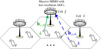
Refer to caption
Fig. 1: Illustration of the multicell massive MIMO network with low-resolution ADCs at the BS.

It is assumed that the ADC pairs related to antenna mm at BS jj has bj,mb_{j,m} quantization bits. Thus, 𝐘jp\mathbf{Y}^{p}_{j} is quantized by

𝐘~jp=𝒬⁡(𝐘jp),\tilde{\mathbf{Y}}^{p}_{j}=\mathcal{Q}(\mathbf{Y}^{p}_{j}), (3)

where 𝒬⁡(𝐘jp)\mathcal{Q}(\mathbf{Y}^{p}_{j}) is an element-wise quantization applied to the real and imaginary parts of 𝐘jp\mathbf{Y}^{p}_{j}, respectively. Obeying to the majority of works [7, 8, 9, 10, 11, 12, 13, 14, 15, 16, 17, 18, 19, 20, 21, 22, 23, 24, 25, 26, 27, 28], we also adopt the AQNM to obtain a linearized approximation of the quantization 𝒬⁡(𝐘jp)\mathcal{Q}(\mathbf{Y}^{p}_{j}) . Under the consideration of AQNM, the quantized version of 𝐘jp\mathbf{Y}^{p}_{j} can further be given by

𝐘~jp=𝒬⁡(𝐘jp)=𝚺jAD​𝐘jp+𝐐jp,\tilde{\mathbf{Y}}^{p}_{j}=\mathcal{Q}(\mathbf{Y}^{p}_{j})=\bm{\Sigma}^{\mathrm{AD}}_{j}\mathbf{Y}^{p}_{j}+\mathbf{Q}^{p}_{j}, (4)

where 𝚺jAD=diag⁡(αi,1AD,⋯,αi,MAD)\bm{\Sigma}^{\mathrm{AD}}_{j}=\mathrm{diag}(\alpha^{\mathrm{AD}}_{i,1},\cdots,\alpha^{\mathrm{AD}}_{i,M}) denotes the distortion matrix determined by the ADCs at BS jj. If the quantization bits of antenna mm at BS jj is bj,mADb^{\mathrm{AD}}_{j,m}, the values of distortion factor αj,mAD\alpha_{j,m}^{\mathrm{AD}} are exemplified in Table I for bj,mAD⩽5b_{j,m}^{\mathrm{AD}}\leqslant 5. When bj,mAD>5b_{j,m}^{\mathrm{AD}}>5, αm,nAD\alpha_{m,n}^{\mathrm{AD}} is approximated as αj,mAD≈1−π​32​2−2​bj,mAD\alpha_{j,m}^{\mathrm{AD}}\approx 1-\frac{\pi\sqrt{3}}{2}2^{-2b_{j,m}^{\mathrm{AD}}}. Moreover, 𝐐jp\mathbf{Q}^{p}_{j} in (4) denotes the quantization noise which is uncorrelated with 𝐘jp\mathbf{Y}^{p}_{j} and each column of 𝐐jp\mathbf{Q}^{p}_{j} is assumed to follow the complex Gaussian distribution with zero mean and variance of

𝐑𝐪jp=1τp​𝚺jAD​(𝐈M−𝚺jAD)​diag​(𝔼⁡{𝐘jp​(𝐘jp)H})=𝚺jAD​(𝐈M−𝚺jAD)​diag​(∑i=1L𝐇j,i​𝐏i​𝐇j,iH+σ2​𝐈M).\begin{split}&\mathbf{R}_{\mathbf{q}^{p}_{j}}=\frac{1}{\tau_{p}}\bm{\Sigma}^{\mathrm{AD}}_{j}(\mathbf{I}_{M}-\bm{\Sigma}^{\mathrm{AD}}_{j})\mathrm{diag}(\mathbb{E}\{\mathbf{Y}^{p}_{j}(\mathbf{Y}^{p}_{j})^{H}\})\\ &=\bm{\Sigma}^{\mathrm{AD}}_{j}(\mathbf{I}_{M}-\bm{\Sigma}^{\mathrm{AD}}_{j})\mathrm{diag}\left(\sum_{i=1}^{L}\mathbf{H}_{j,i}\mathbf{P}_{i}\mathbf{H}_{j,i}^{H}+\sigma^{2}\mathbf{I}_{M}\right).\end{split} (5)
TABLE I: Values of αj,mAD\alpha_{j,m}^{\mathrm{AD}} for bj,mAD≤5b_{j,m}^{\mathrm{AD}}\leq 5[32, 28].
bj,mADb_{j,m}^{\mathrm{AD}} 1 2 3 4 5
αj,mAD\alpha_{j,m}^{\mathrm{AD}} 0.6366 0.8825 0.96546 0.990503 0.997501

II-B Uplink Data Transmission

During this phase, all users in each cell intend to transmit their uplink signal to the corresponding BS. Suppose that 𝐬i\mathbf{s}_{i} is the symbols vector of the users in cell ii and that 𝐬i\mathbf{s}_{i} has zero mean and unit variance for all i=1,⋯,Li=1,\cdots,L. Then the received signal at BS jj is expressed as

𝐲j=𝐇j,j​𝐏j1/2​𝐬j+∑i≠jL𝐇j,i​𝐏i1/2​𝐬i+𝐧j,\mathbf{y}_{j}=\mathbf{H}_{j,j}\mathbf{P}_{j}^{1/2}\mathbf{s}_{j}+\sum_{i\neq j}^{L}\mathbf{H}_{j,i}\mathbf{P}_{i}^{1/2}\mathbf{s}_{i}+\mathbf{n}_{j}, (6)

where 𝐧j\mathbf{n}_{j}, which follows 𝒞​𝒩​(𝟎,σ2​𝐈M)\mathcal{CN}(\mathbf{0},\sigma^{2}\mathbf{I}_{M}), is the AWGN vector at BS jj. The second term of the RHS in (6) represents the interference from the users in the other cells.

Suppose that the same ADC architecture is utilized for both uplink pilot and data transmissions. In that case, similarly to the stage of uplink pilot transmission, we also resort to the AQNM and thus obtain the quantized version of 𝐲j\mathbf{y}_{j} via

𝐲~j=𝒬⁡(𝐲j)=𝚺jAD​𝐲j+𝐪j,\tilde{\mathbf{y}}_{j}=\mathcal{Q}(\mathbf{y}_{j})=\bm{\Sigma}^{\mathrm{AD}}_{j}\mathbf{y}_{j}+\mathbf{q}_{j}, (7)

where 𝐪j\mathbf{q}_{j} is the quantization noise which is uncorrelated with 𝐲j\mathbf{y}_{j}. Note that 𝐪j\mathbf{q}_{j} is also assumed to follow the complex Gaussian distribution with zero mean and variance of

𝐑𝐪j=𝚺jAD​(𝐈M−𝚺jAD)​diag​(𝔼⁡{𝐲j​(𝐲j)H})=𝚺jAD​(𝐈M−𝚺jAD)​diag​(∑i=1L𝐇j,i​𝐏i​𝐇j,iH+σ2​𝐈M).\begin{split}&\mathbf{R}_{\mathbf{q}_{j}}=\bm{\Sigma}^{\mathrm{AD}}_{j}(\mathbf{I}_{M}-\bm{\Sigma}^{\mathrm{AD}}_{j})\mathrm{diag}(\mathbb{E}\{\mathbf{y}_{j}(\mathbf{y}_{j})^{H}\})\\ &=\bm{\Sigma}^{\mathrm{AD}}_{j}(\mathbf{I}_{M}-\bm{\Sigma}^{\mathrm{AD}}_{j})\mathrm{diag}\left(\sum_{i=1}^{L}\mathbf{H}_{j,i}\mathbf{P}_{i}\mathbf{H}_{j,i}^{H}+\sigma^{2}\mathbf{I}_{M}\right).\end{split} (8)

III Uplink Channel Estimation

Since channel estimation is a prerequisite for coherent detection, in this section, we will develop a quantization-aware estimator to obtain CSI. In practical systems, symbols reserved for uplink training in one coherence block are inadequate under large LL and KK so one pilot set might be reused in different cells. We use 𝒫j,k\mathcal{P}_{j,k} to denote the set of all users that utilize the same pilot sequence as user kk in cell jj. On this basis, 𝒫j,k\mathcal{P}_{j,k} is mathematically defined as

𝒫j,k={(i,k′):ϕi,k′=ϕj,k,i=1,⋯,L,k′=1,⋯,K}.\mathcal{P}_{j,k}=\{(i,k^{\prime}):\bm{\phi}_{i,k^{\prime}}=\bm{\phi}_{j,k},i=1,\cdots,L,k^{\prime}=1,\cdots,K\}. (9)

Suppose that BS jj intends to estimate the channel 𝐡j,i​k\mathbf{h}_{j,ik} from an arbitrary user kk in cell ii. 33 3 When i=ji=j, BS jj will estimate the channels of its own users. The BS can correlate 𝐘~jp\tilde{\mathbf{Y}}^{p}_{j} with the pilot sequence ϕi,k\bm{\phi}_{i,k} associated with this user. As a result, the processed received pilot signal is 𝐲~j,i​kp=𝐘~jp​ϕi,k\tilde{\mathbf{y}}^{p}_{j,ik}=\tilde{\mathbf{Y}}^{p}_{j}\bm{\phi}_{i,k}, which is expanded into

𝐲~j,i​kp=pi,k​τp​𝚺jAD​𝐡j,i​k+∑(l,k′)∈𝒫i,k\(i,k)pl,k′​τp​𝚺jAD​𝐡j,l​k′+𝚺jAD​𝐍jp​ϕi,k+𝐐jp​ϕi,k.\begin{split}\tilde{\mathbf{y}}^{p}_{j,ik}&=\sqrt{p_{i,k}}\tau_{p}\bm{\Sigma}^{\mathrm{AD}}_{j}\mathbf{h}_{j,ik}+\sum_{(l,k^{\prime})\in\mathcal{P}_{i,k}\backslash(i,k)}\sqrt{p_{l,k^{\prime}}}\tau_{p}\bm{\Sigma}^{\mathrm{AD}}_{j}\mathbf{h}_{j,lk^{\prime}}\\ &+\bm{\Sigma}^{\mathrm{AD}}_{j}\mathbf{N}^{p}_{j}\bm{\phi}_{i,k}+\mathbf{Q}^{p}_{j}\bm{\phi}_{i,k}.\end{split} (10)

The second term of the RHS in (10) denotes the pilot contamination produced by the users in 𝒫j,k\mathcal{P}_{j,k} except user kk in cell jj. Besides, in (10), it holds that 𝐍jp​ϕi,k∼𝒞​𝒩​(𝟎,σ2​τp​𝐈M)\mathbf{N}^{p}_{j}\bm{\phi}_{i,k}\thicksim\mathcal{CN}(\mathbf{0},\sigma^{2}\tau_{p}\mathbf{I}_{M}) and 𝐐jp​ϕi,k∼𝒞​𝒩​(𝟎,τp​𝐑𝐪jp)\mathbf{Q}^{p}_{j}\bm{\phi}_{i,k}\thicksim\mathcal{CN}(\mathbf{0},\tau_{p}\mathbf{R}_{\mathbf{q}^{p}_{j}}).

In what follows, we will investigate the estimation process for 𝐡j,i​k\mathbf{h}_{j,ik} based on 𝐲~j,i​kp\tilde{\mathbf{y}}^{p}_{j,ik}. By referring to [34] and taking the impact of quantization into account, the quantization-aware MMSE estimate of 𝐡j,i​k\mathbf{h}_{j,ik} is given by

𝐡^j,i​k=pi,k​𝐑j,i​k​𝚺jAD​𝚿j,i​k​𝐲~j,i​kp,\hat{\mathbf{h}}_{j,ik}=\sqrt{p_{i,k}}\mathbf{R}_{j,ik}\bm{\Sigma}^{\mathrm{AD}}_{j}\bm{\Psi}_{j,ik}\tilde{\mathbf{y}}^{p}_{j,ik}, (11)

where

𝚿j,i​k=(∑(l,k′)∈𝒫i,k\(i,k)pl,k′​τp​𝚺jAD​𝐑j,l​k′​𝚺jAD+𝐙jp)−1\bm{\Psi}_{j,ik}=\left(\sum_{(l,k^{\prime})\in\mathcal{P}_{i,k}\backslash(i,k)}p_{l,k^{\prime}}\tau_{p}\bm{\Sigma}^{\mathrm{AD}}_{j}\mathbf{R}_{j,lk^{\prime}}\bm{\Sigma}^{\mathrm{AD}}_{j}+\mathbf{Z}_{j}^{p}\right)^{-1} (12)

with 𝐙jp=σ2​(𝚺jAD)2+𝐑¯𝐪jp\mathbf{Z}_{j}^{p}=\sigma^{2}(\bm{\Sigma}^{\mathrm{AD}}_{j})^{2}+\bar{\mathbf{R}}_{\mathbf{q}^{p}_{j}}. It is worthwhile to mention that

𝐑¯𝐪jp=𝚺jAD​(𝐈M−𝚺jAD)​diag​(∑i=1L∑k=1Kpi,k​𝐑j,i​k+σ2​𝐈M)\bar{\mathbf{R}}_{\mathbf{q}^{p}_{j}}=\bm{\Sigma}^{\mathrm{AD}}_{j}(\mathbf{I}_{M}-\bm{\Sigma}^{\mathrm{AD}}_{j})\mathrm{diag}\left(\sum_{i=1}^{L}\sum_{k=1}^{K}p_{i,k}\mathbf{R}_{j,ik}+\sigma^{2}\mathbf{I}_{M}\right) (13)

is the approximation of 𝐑𝐪jp{\mathbf{R}}_{\mathbf{q}^{p}_{j}}. We here use 𝐑¯𝐪jp\bar{\mathbf{R}}_{\mathbf{q}^{p}_{j}} rather than 𝐑𝐪jp{\mathbf{R}}_{\mathbf{q}^{p}_{j}} because the perfect CSI in (5) is unavailable during the stage of channel estimation and only the spatial correlation matrix 𝐑j,i​k\mathbf{R}_{j,ik} is assumed to be known at the BSs.

According to the linear MMSE estimate theory in [34], the estimation error is modeled as 𝐡~j,i​k=𝐡j,i​k−𝐡^j,i​k\tilde{\mathbf{h}}_{j,ik}={\mathbf{h}}_{j,ik}-\hat{\mathbf{h}}_{j,ik}. Moreover, the variance matrices of 𝐡^j,i​k\hat{\mathbf{h}}_{j,ik} and 𝐡~j,i​k\tilde{\mathbf{h}}_{j,ik} are, respectively, calculated as

𝐁j,i​k=𝔼⁡{𝐡^j,i​k​𝐡^j,i​kH}=pi,k​τp​𝐑j,i​k​𝚺jAD​𝚿j,i​k​𝚺jAD​𝐑j,i​k,\mathbf{B}_{j,ik}=\mathbb{E}\{\hat{\mathbf{h}}_{j,ik}\hat{\mathbf{h}}^{H}_{j,ik}\}=p_{i,k}\tau_{p}\mathbf{R}_{j,ik}\bm{\Sigma}^{\mathrm{AD}}_{j}\bm{\Psi}_{j,ik}\bm{\Sigma}^{\mathrm{AD}}_{j}\mathbf{R}_{j,ik}, (14)

and

𝐂j,i​k=𝔼⁡{𝐡~j,i​k​𝐡~j,i​kH}=𝐑j,i​k−𝐁j,i​k.\mathbf{C}_{j,ik}=\mathbb{E}\{\tilde{\mathbf{h}}_{j,ik}\tilde{\mathbf{h}}^{H}_{j,ik}\}=\mathbf{R}_{j,ik}-\mathbf{B}_{j,ik}. (15)

The estimation quality is evaluated by the normalized MSE, which is given by

𝖭𝖬𝖲𝖤j,i​k=tr⁡(𝐂j,i​k)tr⁡(𝐑j,i​k).\mathsf{NMSE}_{j,ik}=\frac{\mathrm{tr}(\mathbf{C}_{j,ik})}{\mathrm{tr}(\mathbf{R}_{j,ik})}. (16)

If user kk in cell ii uses the same pilot sequence as user k′k^{\prime} in cell i′i^{\prime} and 𝐑j,i​k\mathbf{R}_{j,ik} is invertible, then we have

𝐡^j,i′​k′=pi′,k′pi,k​𝐑j,i′​k′​(𝐑j,i​k)−1​𝐡^j,i​k.\hat{\mathbf{h}}_{j,i^{\prime}k^{\prime}}=\frac{\sqrt{p_{i^{\prime},k^{\prime}}}}{\sqrt{p_{i,k}}}\mathbf{R}_{j,i^{\prime}k^{\prime}}(\mathbf{R}_{j,ik})^{-1}\hat{\mathbf{h}}_{j,ik}. (17)

This implies that 𝐡^j,i′​k′\hat{\mathbf{h}}_{j,i^{\prime}k^{\prime}} and 𝐡^j,i​k\hat{\mathbf{h}}_{j,ik} are correlated with each other and leads to

𝔼⁡{𝐡^j,i′​k′​𝐡^j,i​kH}=pi′,k′pi,k​𝐑j,i′​k′​(𝐑j,i​k)−1​𝐁j,i​k,\mathbb{E}\{\hat{\mathbf{h}}_{j,i^{\prime}k^{\prime}}\hat{\mathbf{h}}^{H}_{j,ik}\}=\frac{\sqrt{p_{i^{\prime},k^{\prime}}}}{\sqrt{p_{i,k}}}\mathbf{R}_{j,i^{\prime}k^{\prime}}(\mathbf{R}_{j,ik})^{-1}\mathbf{B}_{j,ik}, (18)

which will be used in the sequel.

IV Analysis on Spectral and Energy Efficiency

In this section, we investigate the achievable SE corresponding to the uplink data transmission under different linear receive combiners. Without loss of generality, we merely focus on the SE derivations for user kk in cell jj. Suppose that BS jj selects the combining vector 𝐯j,k\mathbf{v}_{j,k}, depending on the estimated channels obtained from the uplink pilot transmission, to recover the desired information of its kkth user. By doing so, BS jj correlates the quantized signal 𝐲~j\tilde{\mathbf{y}}_{j} in (7) to obtain s^j,k=𝐯j,kH​(𝚺jAD)−1​𝐲~j\hat{s}_{j,k}=\mathbf{v}_{j,k}^{H}(\bm{\Sigma}^{\mathrm{AD}}_{j})^{-1}\tilde{\mathbf{y}}_{j}, which can be unfolded into

s^j,k=pj,k​𝔼​{𝐯j,kH​𝐡^j,j​kH​sj,k}⏟Desired​signal+pj,k​(𝐯j,kH​𝐡^j,j​kH​sj,k−𝔼⁡{𝐯j,kH​𝐡^j,j​kH​sj,k})⏟Uncertainty​of​desired​signal+∑k′≠kKpj,k′​𝐯j,kH​𝐡^j,j​k′H​sj,k′⏟Intra−cell​interference+∑i≠jL∑k′=1Kpi,k′​𝐯j,kH​𝐡^j,i​k′H​si,k′⏟Inter−cell​interference+∑i=1L∑k′=1Kpi,k′​𝐯j,kH​𝐡~j,i​k′H​si,k′⏟Interference​from​estimation​error+𝐯j,kH​𝐧j⏟Noise+𝐯j,kH​(𝚺jAD)−1​𝐪j⏟Quantization​noise.\begin{split}\hat{s}_{j,k}&=\underbrace{\sqrt{p_{j,k}}\mathbb{E}\{\mathbf{v}_{j,k}^{H}\hat{\mathbf{h}}_{j,jk}^{H}s_{j,k}\}}_{\mathrm{Desired\,signal}}\\ &+\underbrace{\sqrt{p_{j,k}}(\mathbf{v}_{j,k}^{H}\hat{\mathbf{h}}_{j,jk}^{H}s_{j,k}-\mathbb{E}\{\mathbf{v}_{j,k}^{H}\hat{\mathbf{h}}_{j,jk}^{H}s_{j,k}\})}_{\mathrm{Uncertainty\,of\,desired\,signal}}\\ &+\underbrace{\sum_{k^{\prime}\neq k}^{K}\sqrt{p_{j,k^{\prime}}}\mathbf{v}_{j,k}^{H}\hat{\mathbf{h}}_{j,jk^{\prime}}^{H}s_{j,k^{\prime}}}_{\mathrm{Intra-cell\,interference}}\\ &+\underbrace{\sum_{i\neq j}^{L}\sum_{k^{\prime}=1}^{K}\sqrt{p_{i,k^{\prime}}}\mathbf{v}_{j,k}^{H}\hat{\mathbf{h}}_{j,ik^{\prime}}^{H}s_{i,k^{\prime}}}_{\mathrm{Inter-cell\,interference}}\\ &+\underbrace{\sum_{i=1}^{L}\sum_{k^{\prime}=1}^{K}\sqrt{p_{i,k^{\prime}}}\mathbf{v}_{j,k}^{H}\tilde{\mathbf{h}}_{j,ik^{\prime}}^{H}s_{i,k^{\prime}}}_{\mathrm{Interference\,from\,estimation\,error}}\\ &+\underbrace{\mathbf{v}_{j,k}^{H}\mathbf{n}_{j}}_{\mathrm{Noise}}+\underbrace{\mathbf{v}_{j,k}^{H}(\bm{\Sigma}^{\mathrm{AD}}_{j})^{-1}\mathbf{q}_{j}}_{\mathrm{Quantization\,noise}}.\end{split} (19)

In the RHS of (19), the term pj,k​𝔼​{𝐯j,kH​𝐡^j,j​kH​sj,k}\sqrt{p_{j,k}}\mathbb{E}\{\mathbf{v}_{j,k}^{H}\hat{\mathbf{h}}_{j,jk}^{H}s_{j,k}\} 44 4 We do not use the instantaneous pj,k​𝐯j,kH​𝐡^j,j​kH​sj,k\sqrt{p_{j,k}}\mathbf{v}_{j,k}^{H}\hat{\mathbf{h}}_{j,jk}^{H}s_{j,k} but only its statistics pj,k​𝔼​{𝐯j,kH​𝐡^j,j​kH​sj,k}\sqrt{p_{j,k}}\mathbb{E}\{\mathbf{v}_{j,k}^{H}\hat{\mathbf{h}}_{j,jk}^{H}s_{j,k}\}. The main reason is that the statistics is easy to compute given the statistical property and can be easily acquired over a long-time scale in practical systems. is treated as true desired signal. The other terms of the RHS in (19) can be regarded as effective noise. According to the use-and-then-forget (UatF) bound 55 5 As approved in [35], log2⁡(1+𝔼⁡{X}/𝔼⁡{Y})\log_{2}(1+\mathbb{E}\{X\}/\mathbb{E}\{Y\}) is a lower bound of 𝔼⁡{log2⁡(1+X/Y)}\mathbb{E}\{\log_{2}(1+X/Y)\}. Moreover, when XX and YY are both the sums of the nonnegative random variables and M→∞M\rightarrow\infty, the common approximation 𝔼⁡{log2⁡(1+X/Y)}≈log2⁡(1+𝔼⁡{X}/𝔼⁡{Y})\mathbb{E}\{\log_{2}(1+X/Y)\}\thickapprox\log_{2}(1+\mathbb{E}\{X\}/\mathbb{E}\{Y\}) is tight. mentioned in [1] and [2], the achievable uplink SE (a.k.a the achievable uplink rate) of user kk in cell jj is lower bounded by

𝖲𝖤j,k=τuτc​log2⁡(1+Aj,kBj,k+Cj,k+Dj,k+Ej,k+Fj,k+Gj,k),\mathsf{SE}_{j,k}=\frac{\tau_{u}}{\tau_{c}}\log_{2}(1+\frac{A_{j,k}}{B_{j,k}+C_{j,k}+D_{j,k}+E_{j,k}+F_{j,k}+G_{j,k}}), (20)

in which

Aj,k=pj,k​|𝔼⁡{𝐯j,kH​𝐡^j,j​k}|2,A_{j,k}=p_{j,k}|\mathbb{E}\{\mathbf{v}_{j,k}^{H}\hat{\mathbf{h}}_{j,jk}\}|^{2}, (21)
Bj,k=pj,k​𝔼​{|𝐯j,kH​𝐡^j,j​k|2}−Aj,k,B_{j,k}=p_{j,k}\mathbb{E}\{|\mathbf{v}_{j,k}^{H}\hat{\mathbf{h}}_{j,jk}|^{2}\}-A_{j,k}, (22)
Cj,k=∑k′≠kKpj,k′​𝔼​{|𝐯j,kH​𝐡^j,j​k′|2}C_{j,k}=\sum_{k^{\prime}\neq k}^{K}p_{j,k^{\prime}}\mathbb{E}\{|\mathbf{v}_{j,k}^{H}\hat{\mathbf{h}}_{j,jk^{\prime}}|^{2}\} (23)
Dj,k=∑i≠jL∑k′=1Kpi,k′​𝔼​{|𝐯j,kH​𝐡^j,i​k′|2},D_{j,k}=\sum_{i\neq j}^{L}\sum_{k^{\prime}=1}^{K}p_{i,k^{\prime}}\mathbb{E}\{|\mathbf{v}_{j,k}^{H}\hat{\mathbf{h}}_{j,ik^{\prime}}|^{2}\}, (24)
Ej,k=∑i=1L∑k′=1Kpi,k′​𝔼​{|𝐯j,kH​𝐡~j,i​k′|2},E_{j,k}=\sum_{i=1}^{L}\sum_{k^{\prime}=1}^{K}p_{i,k^{\prime}}\mathbb{E}\{|\mathbf{v}_{j,k}^{H}\tilde{\mathbf{h}}_{j,ik^{\prime}}|^{2}\}, (25)
Fj,k=σ2​𝔼​{‖𝐯j,k‖2},F_{j,k}=\sigma^{2}\mathbb{E}\{||\mathbf{v}_{j,k}||^{2}\}, (26)
Gj,k=𝔼⁡{𝐯j,kH​(𝚺jAD)−1​𝐑𝐪j​(𝚺jAD)−1​𝐯j,k}.G_{j,k}=\mathbb{E}\{\mathbf{v}_{j,k}^{H}(\bm{\Sigma}^{\mathrm{AD}}_{j})^{-1}\mathbf{R}_{\mathbf{q}_{j}}(\bm{\Sigma}^{\mathrm{AD}}_{j})^{-1}\mathbf{v}_{j,k}\}. (27)

All the expectations are with respect to the channel realizations. In what follows, we will derive the asymptotic SEs for three linear combiners.

IV-A Asymptotic Spectral Efficiency of MRC

If MR combining is used, it follows that 𝐯j,k=𝐡^j,j​k\mathbf{v}_{j,k}=\hat{\mathbf{h}}_{j,jk}. Based on the MMSE estimator in Section III, we have the following Theorem 1.

Theorem 1

For MR combining, the terms within the logarithm of (20) can be obtained in closed form. In particular, Aj,kA_{j,k} and Fj,kF_{j,k} are given by (28) and (31), respectively. Bj,k+Cj,k+Dj,k+Ej,kB_{j,k}+C_{j,k}+D_{j,k}+E_{j,k} and Gj,kG_{j,k} are, respectively, given by (29) and (30) at the top of next page.

Aj,k=pj,k​|tr⁡(𝐁j,j​k)|2,A_{j,k}=p_{j,k}\left|\mathrm{tr}(\mathbf{B}_{j,jk})\right|^{2}, (28)
Bj,k+Cj,k+Dj,k+Ej,k=∑i=1L∑k′=1Kpi,k′​(tr⁡(𝐁j,j​k​𝐑j,i​k′)+∑(i,k′)∈𝒫j,kpi,k′2​pj,k​τp2​|tr⁡(𝐑j,i​k′​𝚺jAD​𝚿j,j​k​𝚺jAD​𝐑j,j​k)|2−Aj,kCLOSE,B_{j,k}+C_{j,k}+D_{j,k}+E_{j,k}=\sum_{i=1}^{L}\sum_{k^{\prime}=1}^{K}p_{i,k^{\prime}}(\mathrm{tr}(\mathbf{B}_{j,jk}\mathbf{R}_{j,ik^{\prime}})+\sum_{(i,k^{\prime})\in\mathcal{P}_{j,k}}p^{2}_{i,k^{\prime}}p_{j,k}\tau_{p}^{2}|\mathrm{tr}(\mathbf{R}_{j,ik^{\prime}}\bm{\Sigma}^{\mathrm{AD}}_{j}\bm{\Psi}_{j,jk}\bm{\Sigma}^{\mathrm{AD}}_{j}\mathbf{R}_{j,jk})|^{2}-A_{j,k}, (29)
Gj,k=∑(i,k′)∈𝒫j,k∑m=1M1−αj,mADαj,mAD​(pi,k′2pj,k​(𝚵)m​m+pi,k′​(𝐂j,i​k′)m​m​(𝐁j,j​k)m​m)+∑(i,k′)∉𝒫j,k∑m=1M1−αj,mADαj,mAD(pi,k′(𝐑j,i​k′)m​m(𝐁j,j​k)m​m)+σ2tr(𝐁j,j​k((𝚺ADj)−1−𝐈M)),\begin{split}G_{j,k}&=\sum_{(i,k^{\prime})\in\mathcal{P}_{j,k}}\sum_{m=1}^{M}\frac{1-\alpha^{\mathrm{AD}}_{j,m}}{\alpha^{\mathrm{AD}}_{j,m}}\bigg(\frac{p^{2}_{i,k^{\prime}}}{p_{j,k}}(\bm{\Xi})_{mm}+p_{i,k^{\prime}}(\mathbf{C}_{j,ik^{\prime}})_{mm}(\mathbf{B}_{j,jk})_{mm}\bigg)\\ &+\sum_{(i,k^{\prime})\notin\mathcal{P}_{j,k}}\sum_{m=1}^{M}\frac{1-\alpha^{\mathrm{AD}}_{j,m}}{\alpha^{\mathrm{AD}}_{j,m}}\bigg(p_{i,k^{\prime}}(\mathbf{R}_{j,ik^{\prime}})_{mm}(\mathbf{B}_{j,jk})_{mm}\bigg)+\sigma^{2}\mathrm{tr}(\mathbf{B}_{j,jk}((\bm{\Sigma}^{\mathrm{AD}}_{j})^{-1}-\mathbf{I}_{M})),\end{split} (30)


Fj,k=σ2​tr​(𝐁j,j​k).F_{j,k}=\sigma^{2}\mathrm{tr}(\mathbf{B}_{j,jk}). (31)

Note in (30) that 𝚵\bm{\Xi} is given by

𝚵=𝐑j,i​k′​(𝐑j,j​k)−1​𝐕j,j​km​(𝐑j,j​k)−1​𝐑j,i​k′.\bm{\Xi}=\mathbf{R}_{j,ik^{\prime}}(\mathbf{R}_{j,jk})^{-1}\mathbf{V}^{m}_{j,jk}(\mathbf{R}_{j,jk})^{-1}\mathbf{R}_{j,ik^{\prime}}. (32)

Moreover, the (m1,m2)(m_{1},m_{2})th component of 𝐕j,j​km\mathbf{V}^{m}_{j,jk} in (32) is given by

(𝐕j,j​km)m1​m2=∑m¯,m¯¯(tm1​m¯​tm2​m¯∗​|tm​m¯¯|2+tm1​m¯​tm​m¯∗​tm2​m¯¯∗​tm​m¯¯),\begin{split}&(\mathbf{V}^{m}_{j,jk})_{m_{1}m_{2}}\\ &=\sum_{\bar{m},\bar{\bar{m}}}\left(t_{m_{1}\bar{m}}t^{\ast}_{m_{2}\bar{m}}|t_{m\bar{\bar{m}}}|^{2}+t_{m_{1}\bar{m}}t^{\ast}_{m\bar{m}}t^{\ast}_{m_{2}\bar{\bar{m}}}t_{m\bar{\bar{m}}}\right),\end{split} (33)

in which tp​qt_{pq} is the (p,q)(p,q)th component of 𝐓=𝐁j,j​k1/2\mathbf{T}=\mathbf{B}_{j,jk}^{1/2}.

Proof:

The proof is available in Appendix B. ∎

Substituting (28) to (30) back into (20) yields the asymptotic closed-form SE for the MR combining.

IV-B Asymptotic Spectral Efficiency of Quantization-Aware Multicell MMSE

If BS jj intends to mitigate interference originating from the users in cell jj except user kk and all users in the other cells and to alleviate the impact of quantization errors, we should design a quantization-aware multicell minimum mean-squared error (QA-M-MMSE) combining 𝐯j,kM\mathbf{v}_{j,k}^{\mathrm{M}}. To this end, when only the estimated CSI are available, it follows that

𝐯j,kM=pj,k​(∑i=1L𝐇^j,i​𝐏i​(𝐇^j,i)H+𝐙jM+σ2​𝐈M)−1​𝐡^j,j​k,\mathbf{v}_{j,k}^{\mathrm{M}}=p_{j,k}\left(\sum_{i=1}^{L}\hat{\mathbf{H}}_{j,i}\mathbf{P}_{i}(\hat{\mathbf{H}}_{j,i})^{H}+\mathbf{Z}_{j}^{\mathrm{M}}+\sigma^{2}\mathbf{I}_{M}\right)^{-1}\hat{\mathbf{h}}_{j,jk}, (34)

in which 𝐇^j,i=[𝐡^j,i​1,⋯,𝐡^j,i​k]\hat{\mathbf{H}}_{j,i}=[\hat{\mathbf{h}}_{j,i1},\cdots,\hat{\mathbf{h}}_{j,ik}] and 𝐙jM=∑i=1L∑k′=1Kpi,k′​𝐂j,i​k′+(𝚺jAD)−1​𝐑¯𝐪j​(𝚺jAD)−1\mathbf{Z}_{j}^{\mathrm{M}}=\sum_{i=1}^{L}\sum_{k^{\prime}=1}^{K}p_{i,k^{\prime}}\mathbf{C}_{j,ik^{\prime}}+(\bm{\Sigma}^{\mathrm{AD}}_{j})^{-1}\bar{\mathbf{R}}_{\mathbf{q}_{j}}(\bm{\Sigma}^{\mathrm{AD}}_{j})^{-1}. It should be pointed out that

𝐑¯𝐪j=𝚺jAD​(𝐈M−𝚺jAD)​diag​(∑i=1L∑k=1Kpi,k​𝐑j,i​k+σ2​𝐈M)\bar{\mathbf{R}}_{\mathbf{q}_{j}}=\bm{\Sigma}^{\mathrm{AD}}_{j}(\mathbf{I}_{M}-\bm{\Sigma}^{\mathrm{AD}}_{j})\mathrm{diag}\left(\sum_{i=1}^{L}\sum_{k=1}^{K}p_{i,k}\mathbf{R}_{j,ik}+\sigma^{2}\mathbf{I}_{M}\right) (35)

is approximately equal to 𝐑𝐪j\mathbf{R}_{\mathbf{q}_{j}}. In comparison with [1], it is obvious that the combining vector in (34) takes into account the effect of quantization errors, i.e., 𝐑¯𝐪j\bar{\mathbf{R}}_{\mathbf{q}_{j}}. Based on the MMSE estimator in Section III, we have the following Theorem 2, which is not provided in [1].

Theorem 2

For the quantization-aware multicell MMSE combining, the terms within the logarithm of (20) can be obtained in closed form as follows.

Aj,k→pj,k​|tr⁡(𝐁j,j​k​𝐓j,j​k)M1+tr⁡(𝐁j,j​k​𝐓j,j​k)M|2,A_{j,k}\rightarrow p_{j,k}\left|\frac{\frac{\mathrm{tr}(\mathbf{B}_{j,jk}\mathbf{T}_{j,jk})}{M}}{1+\frac{\mathrm{tr}(\mathbf{B}_{j,jk}\mathbf{T}_{j,jk})}{M}}\right|^{2}, (36)
Bj,k→0,B_{j,k}\rightarrow 0, (37)
Cj,k→∑k′≠kKpj,k′​tr⁡(𝐁j,j​k​𝐓j,j​k′′)M2|1+tr⁡(𝐁j,j​k​𝐓j,j​k)M|2​|1+tr⁡(𝐁j,j​k′​𝐓j,j​k′)M|2,C_{j,k}\rightarrow\sum_{k^{\prime}\neq k}^{K}\frac{p_{j,k^{\prime}}\frac{\mathrm{tr}(\mathbf{B}_{j,jk}\mathbf{T}^{\prime}_{j,jk^{\prime}})}{M^{2}}}{\left|1+\frac{\mathrm{tr}(\mathbf{B}_{j,jk}\mathbf{T}_{j,jk})}{M}\right|^{2}\left|1+\frac{\mathrm{tr}(\mathbf{B}_{j,jk^{\prime}}\mathbf{T}_{j,jk^{\prime}})}{M}\right|^{2}}, (38)
Dj,k→∑i≠jK∑k′=1Kpj,k′​tr⁡(𝐁j,j​k​𝐓j,i​k′′)M2|1+tr⁡(𝐁j,j​k​𝐓j,j​k)M|2​|1+tr⁡(𝐁j,i​k′​𝐓j,i​k′)M|2,D_{j,k}\rightarrow\sum_{i\neq j}^{K}\sum_{k^{\prime}=1}^{K}\frac{p_{j,k^{\prime}}\frac{\mathrm{tr}(\mathbf{B}_{j,jk}\mathbf{T}^{\prime}_{j,ik^{\prime}})}{M^{2}}}{\left|1+\frac{\mathrm{tr}(\mathbf{B}_{j,jk}\mathbf{T}_{j,jk})}{M}\right|^{2}\left|1+\frac{\mathrm{tr}(\mathbf{B}_{j,ik^{\prime}}\mathbf{T}_{j,ik^{\prime}})}{M}\right|^{2}}, (39)
Ej,k→∑i=1K∑k′=1Kpj,k′​tr⁡(𝐁j,j​k​𝐓~j,i​k′′)M2|1+tr⁡(𝐁j,j​k​𝐓j,j​k)M|2,E_{j,k}\rightarrow\sum_{i=1}^{K}\sum_{k^{\prime}=1}^{K}\frac{p_{j,k^{\prime}}\frac{\mathrm{tr}(\mathbf{B}_{j,jk}\tilde{\mathbf{T}}^{\prime}_{j,ik^{\prime}})}{M^{2}}}{\left|1+\frac{\mathrm{tr}(\mathbf{B}_{j,jk}\mathbf{T}_{j,jk})}{M}\right|^{2}}, (40)
Fj,k→σ2​tr⁡(𝐁j,j​k​𝐓j​k,n′)M2|1+tr⁡(𝐁j,j​k​𝐓j,j​k)M|2,F_{j,k}\rightarrow\frac{\sigma^{2}\frac{\mathrm{tr}(\mathbf{B}_{j,jk}\mathbf{T}^{\prime}_{jk,\mathrm{n}})}{M^{2}}}{\left|1+\frac{\mathrm{tr}(\mathbf{B}_{j,jk}\mathbf{T}_{j,jk})}{M}\right|^{2}}, (41)
Gj,k→tr⁡(𝐁j,j​k​𝐓j​k,q′)M2|1+tr⁡(𝐁j,j​k​𝐓j,j​k)M|2.G_{j,k}\rightarrow\frac{\frac{\mathrm{tr}(\mathbf{B}_{j,jk}\mathbf{T}^{\prime}_{jk,\mathrm{q}})}{M^{2}}}{\left|1+\frac{\mathrm{tr}(\mathbf{B}_{j,jk}\mathbf{T}_{j,jk})}{M}\right|^{2}}. (42)

Moreover, 𝐓j,j​k\mathbf{T}_{j,jk} is obtained via (57) in Lemma 3 by letting 𝐀=𝐁j,j​k\mathbf{A}=\mathbf{B}_{j,jk}, 𝚫i​k′=pi​k′pj​k​𝐁j,i​k′\bm{\Delta}_{ik^{\prime}}=\frac{p_{ik^{\prime}}}{p_{jk}}\mathbf{B}_{j,ik^{\prime}}, 𝐃=𝐙jMpj​k​M\mathbf{D}=\frac{\mathbf{Z}^{\mathrm{M}}_{j}}{p_{jk}M}, and α=σ2pj​k​M\alpha=\frac{\sigma^{2}}{p_{jk}M}. Subsequently, 𝐓j,i​k′′\mathbf{T}^{\prime}_{j,ik^{\prime}}, 𝐓~j,i​k′′\tilde{\mathbf{T}}^{\prime}_{j,ik^{\prime}}, 𝐓j​k,n′\mathbf{T}^{\prime}_{jk,\mathrm{n}}, and 𝐓j​k,q′\mathbf{T}^{\prime}_{jk,\mathrm{q}} are obtained via (59) in Lemma 4 by letting 𝐂=𝐁j,i​k′\mathbf{C}=\mathbf{B}_{j,ik^{\prime}}, 𝐂=𝐂j,i​k′\mathbf{C}=\mathbf{C}_{j,ik^{\prime}}, 𝐂=𝐈M\mathbf{C}=\mathbf{I}_{M}, and 𝐂=(𝚺jAD)−1​𝐑¯𝐪j​(𝚺jAD)−1\mathbf{C}=(\bm{\Sigma}^{\mathrm{AD}}_{j})^{-1}\bar{\mathbf{R}}_{\mathbf{q}_{j}}(\bm{\Sigma}^{\mathrm{AD}}_{j})^{-1}, respectively.

Proof:

The proof is available in Appendix C. ∎

Plugging (36) to (42) into (20) gives the asymptotic closed-form SE for the quantization-aware M-MMSE combining.

IV-C Asymptotic Spectral Efficiency of Quantization-Aware Single-cell MMSE

Although the quantization-aware multicell MMSE combining can, to a certain extent, suppress the interference from other interfering users, this scheme needs to estimate the CSI between the BS in a considered cell and the users in other cells. This might give rise to high computational complexity and complicated implementation. If BS jj only estimates the channels relating to its own users, we develop a quantization-aware single-cell minimum mean-squared error (QA-S-MMSE) combining 𝐯j,kS\mathbf{v}_{j,k}^{\mathrm{S}}, which is expressed as

𝐯j,kS=pj,k​(𝐇^j,j​𝐏j​(𝐇^j,j)H+𝐙jS+σ2​𝐈M)−1​𝐡^j,j​k,\mathbf{v}_{j,k}^{\mathrm{S}}=p_{j,k}\left(\hat{\mathbf{H}}_{j,j}\mathbf{P}_{j}(\hat{\mathbf{H}}_{j,j})^{H}+\mathbf{Z}_{j}^{\mathrm{S}}+\sigma^{2}\mathbf{I}_{M}\right)^{-1}\hat{\mathbf{h}}_{j,jk}, (43)

where 𝐙jS=∑i≠jL∑k′=1Kpi,k′​𝐑j,i​k′+∑k′=1Kpj,k′​𝐂j,j​k′+(𝚺jAD)−1​𝐑¯𝐪j​(𝚺jAD)−1\mathbf{Z}_{j}^{\mathrm{S}}=\sum_{i\neq j}^{L}\sum_{k^{\prime}=1}^{K}p_{i,k^{\prime}}\mathbf{R}_{j,ik^{\prime}}+\sum_{k^{\prime}=1}^{K}p_{j,k^{\prime}}\mathbf{C}_{j,jk^{\prime}}+(\bm{\Sigma}^{\mathrm{AD}}_{j})^{-1}\bar{\mathbf{R}}_{\mathbf{q}_{j}}(\bm{\Sigma}^{\mathrm{AD}}_{j})^{-1}. Compared with [1], the combining vector 𝐯j,kS\mathbf{v}_{j,k}^{\mathrm{S}} in (43) also takes into consideration the effect of quantization errors, i.e., 𝐑¯𝐪j\bar{\mathbf{R}}_{\mathbf{q}_{j}}. Based on the MMSE estimator in Section III, we have the following Theorem 3, which is not provided in [1].

Theorem 3

For the quantization-aware single-cell MMSE combining, the terms within the logarithm of (20) can be obtained in closed form as follows.

Aj,k→pj,k​|tr⁡(𝐁j,j​k​𝚪j,j​k)M1+tr⁡(𝐁j,j​k​𝚪j,j​k)M|2,A_{j,k}\rightarrow p_{j,k}\left|\frac{\frac{\mathrm{tr}(\mathbf{B}_{j,jk}\bm{\Gamma}_{j,jk})}{M}}{1+\frac{\mathrm{tr}(\mathbf{B}_{j,jk}\bm{\Gamma}_{j,jk})}{M}}\right|^{2}, (44)
Bj,k→0,B_{j,k}\rightarrow 0, (45)
Cj,k→∑k′≠kKpj,k′​tr⁡(𝐁j,j​k​𝚪j,j​k′′)M2|1+tr⁡(𝐁j,j​k​𝚪j,j​k)M|2​|1+tr⁡(𝐁j,j​k′​𝚪j,j​k′)M|2,C_{j,k}\rightarrow\sum_{k^{\prime}\neq k}^{K}\frac{p_{j,k^{\prime}}\frac{\mathrm{tr}(\mathbf{B}_{j,jk}\bm{\Gamma}^{\prime}_{j,jk^{\prime}})}{M^{2}}}{\left|1+\frac{\mathrm{tr}(\mathbf{B}_{j,jk}\bm{\Gamma}_{j,jk})}{M}\right|^{2}\left|1+\frac{\mathrm{tr}(\mathbf{B}_{j,jk^{\prime}}\bm{\Gamma}_{j,jk^{\prime}})}{M}\right|^{2}}, (46)
Dj,k→∑i≠j(i,k′)∈𝒫j,kKpi,k′​|tr⁡(pi​k′pj​k​𝐑j,i​k′​(𝐑j,j​k)−1​𝐁j,j​k​𝚪j,j​k)M1+tr⁡(𝐁j,j​k​𝚪j,j​k)M|2+∑i≠j(i,k′)∉𝒫j,kKpi,k′tr⁡(𝐁j,j​k​𝚪j,i​k′′)M2|1+tr⁡(𝐁j,j​k​𝚪j,j​k)M|2,\begin{split}D_{j,k}&\rightarrow\sum_{\begin{subarray}{c}i\neq j\\ (i,k^{\prime})\in\mathcal{P}_{j,k}\end{subarray}}^{K}p_{i,k^{\prime}}\left|\frac{\frac{\mathrm{tr}\left(\frac{\sqrt{p_{ik^{\prime}}}}{\sqrt{p_{jk}}}\mathbf{R}_{j,ik^{\prime}}(\mathbf{R}_{j,jk})^{-1}\mathbf{B}_{j,jk}\bm{\Gamma}_{j,jk}\right)}{M}}{1+\frac{\mathrm{tr}(\mathbf{B}_{j,jk}\bm{\Gamma}_{j,jk})}{M}}\right|^{2}\\ &+\sum_{\begin{subarray}{c}i\neq j\\ (i,k^{\prime})\notin\mathcal{P}_{j,k}\end{subarray}}^{K}p_{i,k^{\prime}}\frac{\frac{\mathrm{tr}(\mathbf{B}_{j,jk}\bm{\Gamma}^{\prime}_{j,ik^{\prime}})}{M^{2}}}{\left|1+\frac{\mathrm{tr}(\mathbf{B}_{j,jk}\bm{\Gamma}_{j,jk})}{M}\right|^{2}},\end{split} (47)
Ej,k→∑i=1K∑k′=1Kpj,k′​tr⁡(𝐁j,j​k​𝚪~j,i​k′′)M2|1+tr⁡(𝐁j,j​k​𝚪j,j​k)M|2,E_{j,k}\rightarrow\sum_{i=1}^{K}\sum_{k^{\prime}=1}^{K}\frac{p_{j,k^{\prime}}\frac{\mathrm{tr}(\mathbf{B}_{j,jk}\tilde{\bm{\Gamma}}^{\prime}_{j,ik^{\prime}})}{M^{2}}}{\left|1+\frac{\mathrm{tr}(\mathbf{B}_{j,jk}\bm{\Gamma}_{j,jk})}{M}\right|^{2}}, (48)
Fj,k→σ2​tr⁡(𝐁j,j​k​𝚪j​k,n′)M2|1+tr⁡(𝐁j,j​k​𝚪j,j​k)M|2,F_{j,k}\rightarrow\frac{\sigma^{2}\frac{\mathrm{tr}(\mathbf{B}_{j,jk}\bm{\Gamma}^{\prime}_{jk,\mathrm{n}})}{M^{2}}}{\left|1+\frac{\mathrm{tr}(\mathbf{B}_{j,jk}\bm{\Gamma}_{j,jk})}{M}\right|^{2}}, (49)
Gj,k→tr⁡(𝐁j,j​k​𝚪j​k,q′)M2|1+tr⁡(𝐁j,j​k​𝚪j,j​k)M|2.G_{j,k}\rightarrow\frac{\frac{\mathrm{tr}(\mathbf{B}_{j,jk}\bm{\Gamma}^{\prime}_{jk,\mathrm{q}})}{M^{2}}}{\left|1+\frac{\mathrm{tr}(\mathbf{B}_{j,jk}\bm{\Gamma}_{j,jk})}{M}\right|^{2}}. (50)

Moreover, 𝚪j,j​k\bm{\Gamma}_{j,jk} is obtained via (57) in Lemma 3 by letting L=1L=1, 𝐀=𝐁j,j​k\mathbf{A}=\mathbf{B}_{j,jk}, 𝚫j​k′=pj​k′pj​k​𝐁j,j​k′\bm{\Delta}_{jk^{\prime}}=\frac{p_{jk^{\prime}}}{p_{jk}}\mathbf{B}_{j,jk^{\prime}}, 𝐃=𝐙jSpj​k​M\mathbf{D}=\frac{\mathbf{Z}^{\mathrm{S}}_{j}}{p_{jk}M}, and α=σ2pj​k​M\alpha=\frac{\sigma^{2}}{p_{jk}M}. Next, 𝚪j,i​k′′\bm{\Gamma}^{\prime}_{j,ik^{\prime}}, 𝚪~j,i​k′′\tilde{\bm{\Gamma}}^{\prime}_{j,ik^{\prime}}, 𝚪j​k,n′\bm{\Gamma}^{\prime}_{jk,\mathrm{n}}, and 𝚪j​k,q′\bm{\Gamma}^{\prime}_{jk,\mathrm{q}} are obtained via (59) in Lemma 4 by letting 𝐂=𝐁j,i​k′\mathbf{C}=\mathbf{B}_{j,ik^{\prime}}, 𝐂=𝐂j,i​k′\mathbf{C}=\mathbf{C}_{j,ik^{\prime}}, 𝐂=𝐈M\mathbf{C}=\mathbf{I}_{M}, and 𝐂=(𝚺jAD)−1​𝐑¯𝐪j​(𝚺jAD)−1\mathbf{C}=(\bm{\Sigma}^{\mathrm{AD}}_{j})^{-1}\bar{\mathbf{R}}_{\mathbf{q}_{j}}(\bm{\Sigma}^{\mathrm{AD}}_{j})^{-1}, respectively.

Proof:

The proof is available in Appendix D. ∎

By substitution of (44) to (50) back into (20), we get the asymptotic closed-form SE for the quantization-aware S-MMSE combining.

IV-D Energy Efficiency

Refer to caption
Fig. 2: Illustration of the setup with 9 cells located on a square of 3×33\times 3 grid. The cells with same color are use the same pilot.

According to the power consumption model in [21, 36, 28], the energy efficiency is defined mathematically as

ηEE=W​∑j=1L∑k=1K𝖲𝖤j,kPtotal​bits/Joule,\eta_{\mathrm{EE}}=\frac{W\sum_{j=1}^{L}\sum_{k=1}^{K}\mathsf{SE}_{j,k}}{P_{\mathrm{total}}}\mathrm{bits/Joule}, (51)

where PtotalP_{\mathrm{total}} denotes the total power consumption concerning all BSs in a multicell massive MIMO, 𝖲𝖤j,k\mathsf{SE}_{j,k} is given by (20), and WW indicates the transmission bandwidth with W=20W=20 MHz. The power consumption of an ADC with bj,mADb^{\mathrm{AD}}_{j,m} quantization bits is

PADC=3​Vd​d2​Lmin​(2​W+fc​o​r)10−0.1525​bj,mAD+4.838,P_{\mathrm{ADC}}=\frac{3V_{dd}^{2}L_{\mathrm{min}}(2W+f_{cor})}{10^{-0.1525b^{\mathrm{AD}}_{j,m}+4.838}}, (52)

where Vd​d=3V_{dd}=3 is the power supply of a converter, Lmin=0.5×10⁻⁶L_{\mathrm{min}}=0.5\times 10^{-6} represents the minimum channel length under the given CMOS technology, fc​o​r=106f_{cor}=10^{6} denotes the corner frequency of the 1/f1/f noise [21]. In this context, PtotalP_{\mathrm{total}} can be calculated as

Ptotal=L​M​(2​Pmix+Pfilt+Pfilr+PLNA+PIFA)+2​L​Psyn+∑j=1L∑m=1M2​(cj,mAD​PAGC+PADC),\begin{split}P_{\mathrm{total}}&=LM(2P_{\mathrm{mix}}+P_{\mathrm{filt}}+P_{\mathrm{filr}}+P_{\mathrm{LNA}}+P_{\mathrm{IFA}})\\ &+2LP_{\mathrm{syn}}+\sum_{j=1}^{L}\sum_{m=1}^{M}2(c^{\mathrm{AD}}_{j,m}P_{\mathrm{AGC}}+P_{\mathrm{ADC}}),\end{split} (53)

where PmixP_{\mathrm{mix}}, PfiltP_{\mathrm{filt}}, PfilrP_{\mathrm{filr}}, PLNAP_{\mathrm{LNA}}, PIFAP_{\mathrm{IFA}}, PsynP_{\mathrm{syn}}, PAGCP_{\mathrm{AGC}} denote the power consumption pertaining to the mixer, the filters at the transmitter, the filters at the receiver, low noise amplifiers (LNA), the intermediate frequency amplifier (IFA), the frequency synthesizer, and the automatic gain control (AGC), respectively. In addition, cj,mADc^{\mathrm{AD}}_{j,m} is given by

cj,mAD={0,bj,mAD=11,bj,mAD>1,c^{\mathrm{AD}}_{j,m}=\begin{cases}0,&b^{\mathrm{AD}}_{j,m}=1\\ 1,&b^{\mathrm{AD}}_{j,m}>1\end{cases},

which is an indicator describing whether or not antenna mm at BS jj uses 1-bit ADC pair.

V Numerical Results and Discussions

In the simulation to follow, we use a 9-cell setup, as depicted in Fig. 2. Each cell covers a square with area 0.25​km×0.25​km0.25\mathrm{km}\times 0.25\mathrm{km} and is deployed on a square of 3×33\times 3 cells. The large-scale fading coefficient βj,i​k\beta_{j,ik} is modeled as βj,i​k=−148.1​dB−37.6​α​log10⁡(dj,i​k/1​km)\beta_{j,ik}=-148.1\mathrm{dB}-37.6\alpha\log_{10}(d_{j,ik}/1\mathrm{km}), where dj,i​kd_{j,ik} is the distance between BS jj and user kk in cell ii. 55 users are independently and uniformly distributed in each cell, at the center of which there exists a BS with M=30M=30 antennas. We consider communication over 2020 MHz bandwidth and the noise power is −94-94 dBm, including noise figure with 77 dB. Suppose that the local scattering model in [1] is utilized and antenna arrays have half-wavelength spacing. If multipaths arrive from the far-field of the arrays, the (m,n)(m,n)th entry of spatial correlation matrix 𝐑j,i​k\mathbf{R}_{j,ik} can be computed as [1]

[𝐑j,i​k]m​n=βj,i​k​∫ej​π​(m−n)​sin⁡(ψ)​f​(φ¯)​𝑑φ¯,[\mathbf{R}_{j,ik}]_{mn}=\beta_{j,ik}\int e^{\mathrm{j}\pi(m-n)\sin(\psi)}f(\bar{\varphi})\mathrm{d}\bar{\varphi}, (54)

where φ¯\bar{\varphi} denotes the angle of a multipath component. Notice that φ¯=φ+δ\bar{\varphi}={\varphi}+\delta with φ\varphi being a deterministic nominal angle and δ\delta being a random deviation from φ\varphi. It is obvious from (54) that 𝐑j,i​k\mathbf{R}_{j,ik} is a Toeplitz matrix. In the simulation, Gaussian distributed deviation δ∼𝒩⁡(0,σφ2)\delta\thicksim\mathcal{N}(0,\sigma^{2}_{\varphi}) is used. The standard deviation σφ⩾0\sigma_{\varphi}\geqslant 0 is called the angular standard deviation (ASD). Unless stated otherwise, we consider σφ=10∘\sigma_{\varphi}=10^{\circ}, τc=200\tau_{c}=200 samples and τp=f​K\tau_{p}=fK samples with ff being the pilot reuse factor associated with 9-cell setup. In what follows, we let f=3f=3 and the corresponding pilot assignment is shown in Fig. 2. The Monte Carlo simulation results are obtained by averaging instantaneous SE over 100100 realizations of small-scale fading channels and 100100 realizations of the random locations of users, while the asymptotic results are obtained by averaging asymptotic SEs in Theorem 1, Theorem 2, and Theorem 3 over 100100 realizations of the random locations of users, respectively.

Fig. 3: Comparison of achievable SE between simulated results and asymptotic results for QA-M-MMSE and QA-S-MMSE. L=9L=9, M=30M=30, K=5K=5, f=3f=3, and σφ=10∘\sigma_{\varphi}=10^{\circ}.
Fig. 4: Comparison of achievable SE between simulated results and asymptotic results for MRC. L=9L=9, M=30M=30, K=5K=5, f=3f=3, and σφ=10∘\sigma_{\varphi}=10^{\circ}.

Under different quantization bits, Fig. 3 and Fig. 4 compare the asymptotic results and the simulated ones for MMSE-based and MRC combiners, respectively. Note that “Asy.” and “Sim.” represent the asymptotic and simulation results, respectively. It is evident from Fig. 3 that the asymptotic results of QA-M-MMSE and QA-S-MMSE match with the corresponding simulation results in a high degree of accuracy, especially for the case without quantization. Meanwhile, for the MRC, it is observed from Fig. 4 that the asymptotic results substantially coincide with the simulation ones and the gap is inconspicuous. These observations approve the tightness of our asymptotic analyses relating to Theorem 1, Theorem 2, and Theorem 3. Moreover, from the results in Fig. 3, we also observe that the performance of QA-M-MMSE is superior to that of QA-S-MMSE in the case of un-quantization. The main reason is that the QA-M-MMSE can make a trade-off of suppression between intra-cell and inter-cell interference. Instead, the QA-S-MMSE can only mitigate intra-cell interference. However, at the regime of low-resolution ADCs, the performance gap between QA-M-MMSE and QA-S-MMSE shrinks as the quantization bit decreases. The reason is that the interference caused by quantization errors, compared with that produced by other users, is the dominant factor resulting in performance loss, notably under 1-bit quantization.

Fig. 5 exemplifies the estimation quality of quantization-aware and quantization-unaware MMSE estimators in terms of NMSE. It is noticeable that considering the impact of quantization errors can improve the performance of channel estimation, particularly in the high SNR region under low-resolution quantization. The main reason is that the quantization-aware estimator takes into account the variance of quantization noise during channel estimation, as shown in (11) and (12), whereas the quantization-unaware one does not. In addition, we can also observe that increasing transmit power cannot completely compensate the impact of low resolution quantization. When there exist quantization errors, the NMSE approaches to an asymptotic value as we augment the transmit power. This saturation occurs because the interference caused by quantization errors, proportional to the transmit power, dominate the loss of NMSE compared with the thermal noise.

Fig. 5: Performance of channel estimation for quantization-aware and quantization-unaware estimators under different quantization bits. L=9L=9, M=30M=30, K=5K=5, f=3f=3, and σφ=10∘\sigma_{\varphi}=10^{\circ}.
Fig. 6: Achievable SE for quantization-aware and quantization-unaware MMSE-based combiners under different quantization bits. L=9L=9, M=30M=30, K=5K=5, f=3f=3, and σφ=10∘\sigma_{\varphi}=10^{\circ}.

Fig. 6 shows the achievable sum SEs for quantization-aware and quantization-unaware MMSE-based combiners, respectively. Again, we find that considering the impact of quantization errors can ameliorate system performance. The reason is that the proposed quantization-aware MMSE combining can be treated as a spatial whitening filter and is an optimal linear combiner in terms of typical mean-squared error (MSE) criterion. As a result, the impact of the distortion caused by quantization can be alleviated to a certain extent. Moreover, for quantization-unaware MMSE combiners, the S-MMSE is more beneficial than the M-MMSE. The main reason is that the interference caused by higher channel estimation errors dominate the performance loss. In this case, the M-MMSE, which aims to exploit the estimated channel associated with the users in other cells, cannot effectively compensate the interference from other cells under relatively inaccurate channel estimate degraded by quantization errors. Meanwhile, suppressing inter-cell interference is obtained at the cost of reducing the performance of mitigating intra-cell interference.

Fig. 7: Performance of channel estimation for quantization-aware and quantization-unaware estimators under different quantization bits. L=9L=9, M=30M=30, K=5K=5, f=3f=3, and p=30p=30 dBm.
Fig. 8: Achievable SE for quantization-aware and quantization-unaware combiners based on MMSE along with MRC. L=9L=9, M=30M=30, K=5K=5, f=3f=3, and p=30p=30 dBm.

Fig. 7 assesses the performance of channel estimation in terms of NMSE for different channel correlation under the existence of pilot contamination. In the context of un-quantization, we observe that the NMSE reduces as the ASD decreases (i.e., towards higher spatial correlation) for both quantization-aware and quantization-unaware MMSE estimators. In fact, this two estimators are equivalent if there do not exist quantization errors. However, in the case of low-resolution quantization, the NMSE first decreases but then rises as the ASD changes to large degrees. The main reason is explained as follows. On the one hand, strong spatial correlation is beneficial due to the fact that most of the channel’s variance lies in a few eigenvalues when ASD is small and that it is much harder to estimate weaken eigendirections than stronger ones. On the other hand, strong spatial correlation is detrimental because of the fact that the quantization errors are adversely affected by spatial correlation. This implies that there exists an ADS to achieve the optimal NMSE.66 6 This optimal ASD can be found experimentally. In principle, to optimize the ADS is an interesting and challenging topic, which will be left as future work.

Fig. 8 illustrates the achievable sum SEs for different channel correlation under the existence of pilot contamination. We see that the performance is not so good when the spatial channel correlation is strong (with very small ASD). For MMSE-based combiners, the SE first increases but then reduces as the ASD changes to large values. For MRC, the SE increases as the ADS grows large. Regarding these phenomena, one reason is that the UatF bound relies on channel hardening and less hardening occurs when the spatial channel correlation is strong. The other reason is that channel estimate might be inaccurate at the strong spatial correlation and quantization errors, as shown in Fig. 7.

Fig. 9 presents the energy efficiency in conjunction with the trade-off between achievable sum SE and energy efficiency of multicell massive MIMO systems. Based on the existing work [21], the power consumption of different hardware components in (53) are given as Pmix=30.3P_{\mathrm{mix}}=30.3 mW, Pfilt=Pfilr=2.5P_{\mathrm{filt}}=P_{\mathrm{filr}}=2.5 mW, Psyn=50P_{\mathrm{syn}}=50 mW, PLNA=20P_{\mathrm{LNA}}=20 mW, PIFA=3P_{\mathrm{IFA}}=3 mW, PAGC=2P_{\mathrm{AGC}}=2 mW. As the number of quantization bits increases, it can be seen from the left part of Fig. 9 that the energy efficiencies of different combiners rise first but then decrease. This shows that the energy efficiencies of the three combiners have their own peaks, This suggests that it is not always advisable to increase the ADC quantization bits. Moreover, it can be observed from the right part of Fig. 9 that after a specific point slight increase of achievable sum SEs can result in lager decrease of energy efficiency, especially in the case where the achievable sum SEs are achieved under high-resolution ADCs. Based on these observations, it can be concluded that a multicell massive MIMO system with low-resolution ADCs (e.g., 3-5 bits) is more advantageous from the perspective of energy efficiency.

Fig. 9: Energy efficiency versus quantization bits (left) and the trade-off between achievable SE and energy efficiency (right). L=9L=9, M=30M=30, K=5K=5, f=3f=3, σφ=10∘\sigma_{\varphi}=10^{\circ}, and p=30p=30 dBm.

VI Conclusion

In this study, focusing on multicell massive MIMO systems with variable-resolution ADCs and spatially correlated Rayleigh fading channels, we derived the asymptotic closed-form expressions of the achievable uplink SE given that MRC and quantization-aware MMSE combiners are used at the BS. The tightness of our asymptotic analyses, which comprehensively consider the intra-cell and inter-cell interference, estimation errors, quantization noise, and spatial correlation, is validated by simulation results. Among these results, we find that the proposed quantization-aware estimator and combiners are more helpful than the quantization-unaware counterparts. In addition, it is also verified that the performance of QA-M-MMSE outperforms that of QA-S-MMSE via considering the influence of inter-cell interference. Furthermore, we conclude that applying low-resolution ADCs in a multicell massive MIMO system is a promising candidate to achieve high energy efficiency. As future work, we intend to solve optimization problems under the constraints of power consumption and total quantization bits by regarding the asymptotic achievable SEs as objective functions. This is challenging because the quantization bits are discrete integers and the objective functions are non-convex.

Appendix A Basic Lemmas

This appendix provides some basic lemmas that are helpful to derive all the principal SE bounds in this article.

Lemma 1 (Matrix Inversion Lemma)

Suppose that 𝐀\mathbf{A} is a Hermitian invertible matrix and 𝐀+α​𝐛𝐛H\mathbf{A}+\alpha\mathbf{b}\mathbf{b}^{H} is also invertible for any vector 𝐛\mathbf{b} and scalar α\alpha. It holds that

𝐛H​(𝐀+α​𝐛𝐛H)−1=𝐛H​𝐀−11+α​𝐛H​𝐀−1​𝐛.\mathbf{b}^{H}\left(\mathbf{A}+\alpha\mathbf{b}\mathbf{b}^{H}\right)^{-1}=\frac{\mathbf{b}^{H}\mathbf{A}^{-1}}{1+\alpha\mathbf{b}^{H}\mathbf{A}^{-1}\mathbf{b}}. (55)
Lemma 2

Suppose that 𝐀\mathbf{A} has uniformly bounded spectral norm and 𝐱∼𝒞​𝒩​(𝟎,1M​𝐑𝐱)\mathbf{x}\thicksim\mathcal{CN}(\mathbf{0},\frac{1}{M}\mathbf{R}_{\mathbf{x}}). It follows form [37, Theorem 3.4] that 𝐱H​𝐀𝐱→M→∞a.s.1M​tr​(𝐑𝐱​𝐀)\mathbf{x}^{H}\mathbf{A}\mathbf{x}\xrightarrow[M\rightarrow\infty]{a.s.}\frac{1}{M}\mathrm{tr}(\mathbf{R}_{\mathbf{x}}\mathbf{A}).

Lemma 3

Suppose that 𝐇i=[𝐡i​1,⋯,𝐡i​K]∈ℂM×K\mathbf{H}_{i}=[\mathbf{h}_{i1},\cdots,\mathbf{h}_{iK}]\in\mathbb{C}^{M\times K} and 𝐇=[𝐇1,⋯,𝐇L]∈ℂM×L​K\mathbf{H}=[\mathbf{H}_{1},\cdots,\mathbf{H}_{L}]\in\mathbb{C}^{M\times LK} with 𝐡i​k′∼𝒞​𝒩​(𝟎,1M​𝚫i​k′)\mathbf{h}_{ik^{\prime}}\thicksim\mathcal{CN}(\mathbf{0},\frac{1}{M}\mathbf{\Delta}_{ik^{\prime}}) for i=1,⋯,Li=1,\cdots,L and k′=1,⋯,Kk^{\prime}=1,\cdots,K. Suppose that 𝐀∈ℂM×M\mathbf{A}\in\mathbb{C}^{M\times M} and 𝐃∈ℂM×M\mathbf{D}\in\mathbb{C}^{M\times M} are nonnegative definite Hermitian matrices. Moreover, 𝐀\mathbf{A}, 𝐃\mathbf{D}, and 𝚫i​k′\mathbf{\Delta}_{ik^{\prime}} have bounded spectral norms. Then, for any positive α\alpha, it follows from [38, Theorem 1] that

1M​tr​(𝐀​(𝐇𝐇H+𝐃+α​𝐈M)−1)→M→∞a.s.1M​tr​(𝐀​𝚪),\frac{1}{M}\mathrm{tr}\left(\mathbf{A}\left(\mathbf{H}\mathbf{H}^{H}+\mathbf{D}+\alpha\mathbf{I}_{M}\right)^{-1}\right)\xrightarrow[M\rightarrow\infty]{a.s.}\frac{1}{M}\mathrm{tr}\left(\mathbf{A}\bm{\Gamma}\right), (56)

where 𝚪\bm{\Gamma} is given by

𝚪=(1M​∑i=1L∑k′=1K𝚫i​k′1+δi​k′+𝐃+α​𝐈M)−1\bm{\Gamma}=\left(\frac{1}{M}\sum_{i=1}^{L}\sum_{k^{\prime}=1}^{K}\frac{\mathbf{\Delta}_{ik^{\prime}}}{1+\delta_{ik^{\prime}}}+\mathbf{D}+\alpha\mathbf{I}_{M}\right)^{-1} (57)

with δi​k′\delta_{ik^{\prime}} being the solution of fixed-point equation δi​k′=1M​tr​(𝚫i​k′​𝚪)\delta_{ik^{\prime}}=\frac{1}{M}\mathrm{tr}\left(\mathbf{\Delta}_{ik^{\prime}}\bm{\Gamma}\right).

Lemma 4

On the basis of Lemma 3, for a nonnegative definite Hermitian matrix 𝐂∈ℂM×M\mathbf{C}\in\mathbb{C}^{M\times M} with bounded spectral norm, it follows from [38] that

1M​tr​(𝐀​(𝐇𝐇H+𝐃+α​𝐈M)−1​𝐂​(𝐇𝐇H+𝐃+α​𝐈M)−1)→M→∞a.s.1M​tr​(𝐀​𝚪′).\begin{split}&\frac{1}{M}\mathrm{tr}\left(\mathbf{A}\left(\mathbf{H}\mathbf{H}^{H}+\mathbf{D}+\alpha\mathbf{I}_{M}\right)^{-1}\mathbf{C}\left(\mathbf{H}\mathbf{H}^{H}+\mathbf{D}+\alpha\mathbf{I}_{M}\right)^{-1}\right)\\ &\xrightarrow[M\rightarrow\infty]{a.s.}\frac{1}{M}\mathrm{tr}\left(\mathbf{A}\bm{\Gamma}^{\prime}\right).\end{split} (58)

Moreover, 𝚪′\bm{\Gamma}^{\prime} is given by

𝚪′=𝚪​𝐂​𝚪+1M​𝚪​∑i=1L∑k′=1K𝚫i​k′​δi​k′′(1+δi​k′)2​𝚪.\bm{\Gamma}^{\prime}=\bm{\Gamma}\mathbf{C}\bm{\Gamma}+\frac{1}{M}\bm{\Gamma}\sum_{i=1}^{L}\sum_{k^{\prime}=1}^{K}\frac{\mathbf{\Delta}_{ik^{\prime}}\delta_{ik^{\prime}}^{\prime}}{(1+\delta_{ik^{\prime}})^{2}}\bm{\Gamma}. (59)

If letting 𝛅′=[(𝛅1′)T,⋯,(𝛅L′)T]T\bm{\delta}^{\prime}=[(\bm{\delta}^{\prime}_{1})^{T},\cdots,(\bm{\delta}^{\prime}_{L})^{T}]^{T} with 𝛅i′=[δi​1′,⋯,δi​K′]T\bm{\delta}^{\prime}_{i}=[\delta^{\prime}_{i1},\cdots,\delta^{\prime}_{iK}]^{T}, we have 𝛅′=(𝐈L​K−𝐘)−1​𝐱\bm{\delta}^{\prime}=(\mathbf{I}_{LK}-\mathbf{Y})^{-1}\mathbf{x} with the elements of 𝐘∈ℂL​K×L​K\mathbf{Y}\in\mathbb{C}^{LK\times LK} and 𝐱∈ℂL​K×1\mathbf{x}\in\mathbb{C}^{LK\times 1} given by

[𝐘]i​k′,i¯​k¯′=1M​tr​(𝚫i​k′​𝚪​𝚫i¯​k¯′​𝚪)M​(1+δi¯​k¯′)2[\mathbf{Y}]_{ik^{\prime},\bar{i}\bar{k}^{\prime}}=\frac{\frac{1}{M}\mathrm{tr}(\mathbf{\Delta}_{ik^{\prime}}\bm{\Gamma}\mathbf{\Delta}_{\bar{i}\bar{k}^{\prime}}\bm{\Gamma})}{M(1+\delta_{\bar{i}\bar{k}^{\prime}})^{2}} (60)

and

[𝐱]i​k′=1M​tr​(𝚫i​k′​𝚪​𝐂​𝚪).[\mathbf{x}]_{ik^{\prime}}=\frac{1}{M}\mathrm{tr}(\mathbf{\Delta}_{ik^{\prime}}\bm{\Gamma}\mathbf{C}\bm{\Gamma}). (61)
Lemma 5 (Rank-1 Perturbation Lemma)

Suppose that 𝐀∈ℂM×M\mathbf{A}\in\mathbb{C}^{M\times M}, 𝐪∈ℂM×1\mathbf{q}\in\mathbb{C}^{M\times 1}, and that 𝐆∈ℂM×M\mathbf{G}\in\mathbb{C}^{M\times M} is a nonnegative Hermitian matrix. With α\alpha and α′\alpha^{\prime} two given positive real numbers, it follows form [37, Theorem 3.9] that

|tr⁡(𝐀​(𝐆+α​𝐈M)−1−𝐀​(𝐆+α′​𝐠𝐠H+α​𝐈M)−1)|≤‖𝐀‖α.\left|\mathrm{tr}\left(\mathbf{A}(\mathbf{G}+\alpha\mathbf{I}_{M})^{-1}-\mathbf{A}(\mathbf{G}+\alpha^{\prime}\mathbf{g}\mathbf{g}^{H}+\alpha\mathbf{I}_{M})^{-1}\right)\right|\leq\frac{||\mathbf{A}||}{\alpha}. (62)
Lemma 6

Suppose that 𝐚∼𝒞​𝒩​(𝟎,𝐀)\mathbf{a}\thicksim\mathcal{CN}(\mathbf{0},\mathbf{A}) and that 𝐁∈ℂM×M\mathbf{B}\in\mathbb{C}^{M\times M} is a diagonalizable matrix. It holds that

𝔼⁡{|𝐚H​𝐁𝐚|2}=|tr⁡(𝐁𝐀)|2+tr⁡(𝐁𝐀𝐁H​𝐀).\mathbb{E}\{|\mathbf{a}^{H}\mathbf{B}\mathbf{a}|^{2}\}=|\mathrm{tr}(\mathbf{B}\mathbf{A})|^{2}+\mathrm{tr}(\mathbf{B}\mathbf{A}\mathbf{B}^{H}\mathbf{A}). (63)

Appendix B Proof of Theorem 1

It is straightforward to obtain Aj,kA_{j,k} and Fj,kF_{j,k} following Lemma 2. In this appendix, we will derive the closed-form expressions of Ψj,k=Bj,k+Cj,k+Dj,k+Ej,k\Psi_{j,k}=B_{j,k}+C_{j,k}+D_{j,k}+E_{j,k} and Gj,kG_{j,k}.

1) We first deal with Ψj,k\Psi_{j,k}. According to (22)-(25) and 𝐡j,i​k′=𝐡^j,i​k′+𝐡~j,i​k′{\mathbf{h}}_{j,ik^{\prime}}=\hat{\mathbf{h}}_{j,ik^{\prime}}+\tilde{\mathbf{h}}_{j,ik^{\prime}}, it follows that

Ψj,k=∑i=1L∑k′=1Kpi,k′​𝔼​{|𝐯j,kH​𝐡j,i​k′|2}−Aj,k.\Psi_{j,k}=\sum_{i=1}^{L}\sum_{k^{\prime}=1}^{K}p_{i,k^{\prime}}\mathbb{E}\{|\mathbf{v}_{j,k}^{H}\mathbf{h}_{j,ik^{\prime}}|^{2}\}-A_{j,k}. (64)

If we let ψi,k′=𝔼⁡{|𝐯j,kH​𝐡j,i​k′|2}\psi_{i,k^{\prime}}=\mathbb{E}\{|\mathbf{v}_{j,k}^{H}\mathbf{h}_{j,ik^{\prime}}|^{2}\}, the following two cases are discussed because of the pilot contamination.

i) When (i,k′)∉𝒫j,k(i,k^{\prime})\notin\mathcal{P}_{j,k}, 𝐡^j,j​k\hat{\mathbf{h}}_{j,jk} and 𝐡j,i​k′\mathbf{h}_{j,ik^{\prime}} are uncorrelated with each other. In this case, it follows that

ψi,k′=𝔼⁡{|𝐡^j,j​kH​𝐡j,i​k′|2}=𝔼⁡{𝐡^j,j​kH​𝔼​{𝐡j,i​k′​𝐡j,i​k′H}​𝐡^j,j​k}=tr⁡(𝔼⁡{𝐡j,i​k′​𝐡j,i​k′H}​𝔼​{𝐡^j,j​k​𝐡^j,j​kH})=tr⁡(𝐑j,i​k′​𝐁j,j​k).\begin{split}\psi_{i,k^{\prime}}&=\mathbb{E}\{|\hat{\mathbf{h}}_{j,jk}^{H}\mathbf{h}_{j,ik^{\prime}}|^{2}\}\\ &=\mathbb{E}\{\hat{\mathbf{h}}_{j,jk}^{H}\mathbb{E}\{\mathbf{h}_{j,ik^{\prime}}\mathbf{h}_{j,ik^{\prime}}^{H}\}\hat{\mathbf{h}}_{j,jk}\}\\ &=\mathrm{tr}(\mathbb{E}\{\mathbf{h}_{j,ik^{\prime}}\mathbf{h}_{j,ik^{\prime}}^{H}\}\mathbb{E}\{\hat{\mathbf{h}}_{j,jk}\hat{\mathbf{h}}_{j,jk}^{H}\})\\ &=\mathrm{tr}(\mathbf{R}_{j,ik^{\prime}}\mathbf{B}_{j,jk}).\end{split} (65)

ii) When (i,k′)∈𝒫j,k(i,k^{\prime})\in\mathcal{P}_{j,k}, 𝐡^j,j​k\hat{\mathbf{h}}_{j,jk} and 𝐡^j,i​k′\hat{\mathbf{h}}_{j,ik^{\prime}} are uncorrelated with each other. In this regard, ψi,k′\psi_{i,k^{\prime}} can be decomposed as

ψi,k′=𝔼⁡{|𝐡^j,j​kH​𝐡^j,i​k′|2}+𝔼⁡{|𝐡^j,j​kH​𝐡~j,i​k′|2}.\psi_{i,k^{\prime}}=\mathbb{E}\{|\hat{\mathbf{h}}_{j,jk}^{H}\hat{\mathbf{h}}_{j,ik^{\prime}}|^{2}\}+\mathbb{E}\{|\hat{\mathbf{h}}_{j,jk}^{H}\tilde{\mathbf{h}}_{j,ik^{\prime}}|^{2}\}. (66)

We first focus on the first term of the RHS in (66) and let φi,k′=𝔼⁡{|𝐡^j,j​kH​𝐡^j,i​k′|2}\varphi_{i,k^{\prime}}=\mathbb{E}\{|\hat{\mathbf{h}}_{j,jk}^{H}\hat{\mathbf{h}}_{j,ik^{\prime}}|^{2}\}. According to (17), one has

φi,k′=pi,k′pj,k​𝔼​{|𝐡^j,j​kH​𝐑j,i​k′​(𝐑j,j​k)−1​𝐡^j,j​k|2}.\varphi_{i,k^{\prime}}=\frac{{p_{i,k^{\prime}}}}{{p_{j,k}}}\mathbb{E}\left\{\left|\hat{\mathbf{h}}_{j,jk}^{H}\mathbf{R}_{j,ik^{\prime}}(\mathbf{R}_{j,jk})^{-1}\hat{\mathbf{h}}_{j,jk}\right|^{2}\right\}. (67)

Based on Lemma 6, it holds that

φi,k′=pi,k′pj,k[|tr(𝐑j,i​k′(𝐑j,j​k)−1𝐁j,j​k)|2+tr(𝐑j,i​k′(𝐑j,j​k)−1𝐁j,j​k(𝐑j,j​k)−1𝐑j,i​k′𝐁j,j​k)].\begin{split}\varphi_{i,k^{\prime}}&=\frac{{p_{i,k^{\prime}}}}{{p_{j,k}}}\bigg[\left|\mathrm{tr}(\mathbf{R}_{j,ik^{\prime}}(\mathbf{R}_{j,jk})^{-1}\mathbf{B}_{j,jk})\right|^{2}\\ &+\mathrm{tr}(\mathbf{R}_{j,ik^{\prime}}(\mathbf{R}_{j,jk})^{-1}\mathbf{B}_{j,jk}(\mathbf{R}_{j,jk})^{-1}\mathbf{R}_{j,ik^{\prime}}\mathbf{B}_{j,jk})\bigg].\end{split} (68)

Using 𝐁j,i​k′=pi,k′​τp​𝐑j,i​k′​𝚺jAD​𝚿j,i​k′​𝚺jAD​𝐑j,i​k′\mathbf{B}_{j,ik^{\prime}}=p_{i,k^{\prime}}\tau_{p}\mathbf{R}_{j,ik^{\prime}}\bm{\Sigma}^{\mathrm{AD}}_{j}\bm{\Psi}_{j,ik^{\prime}}\bm{\Sigma}^{\mathrm{AD}}_{j}\mathbf{R}_{j,ik^{\prime}} given by (14), φi,k′\varphi_{i,k^{\prime}} can be rewritten as

φi,k′=pi​k′​pj​k​τp2​|tr⁡(𝐑j,i​k′​𝚺jAD​𝚿j,j​k​𝚺jAD​𝐑j,j​k)|2+tr⁡(𝐁j,i​k′​𝐁j,j​k).\begin{split}\varphi_{i,k^{\prime}}&=p_{ik^{\prime}}p_{jk}\tau_{p}^{2}\left|\mathrm{tr}(\mathbf{R}_{j,ik^{\prime}}\bm{\Sigma}^{\mathrm{AD}}_{j}\bm{\Psi}_{j,jk}\bm{\Sigma}^{\mathrm{AD}}_{j}\mathbf{R}_{j,jk})\right|^{2}\\ &+\mathrm{tr}(\mathbf{B}_{j,ik^{\prime}}\mathbf{B}_{j,jk}).\end{split} (69)

Notice that 𝚿j,j​k=𝚿j,i​k′\bm{\Psi}_{j,jk}=\bm{\Psi}_{j,ik^{\prime}} in the case of (i,k′)∈𝒫j,k(i,k^{\prime})\in\mathcal{P}_{j,k}. Next, similarly to the derivation of (65), it holds for the second term of the RHS in (66) that

𝔼⁡{|𝐡^j,j​kH​𝐡~j,i​k′|2}=tr⁡(𝐁j,j​k​𝐂j,i​k′)\mathbb{E}\{|\hat{\mathbf{h}}_{j,jk}^{H}\tilde{\mathbf{h}}_{j,ik^{\prime}}|^{2}\}=\mathrm{tr}(\mathbf{B}_{j,jk}\mathbf{C}_{j,ik^{\prime}}) (70)

since 𝐡^j,i​k′\hat{\mathbf{h}}_{j,ik^{\prime}} and 𝐡~j,i​k′\tilde{\mathbf{h}}_{j,ik^{\prime}} are mutually uncorrelated. Substituting (70) and (69) into (66) with the aid of 𝐑j,i​k′=𝐁j,i​k+𝐂j,i​k′\mathbf{R}_{j,ik^{\prime}}=\mathbf{B}_{j,ik}+\mathbf{C}_{j,ik^{\prime}} leads to

ψi,k′=pi,k′​pj,k​τp2​|tr⁡(𝐑j,i​k′​𝚺jAD​𝚿j,j​k​𝚺jAD​𝐑j,j​k)|2+tr⁡(𝐑j,i​k′​𝐁j,j​k).\begin{split}\psi_{i,k^{\prime}}&=p_{i,k^{\prime}}p_{j,k}\tau_{p}^{2}\left|\mathrm{tr}(\mathbf{R}_{j,ik^{\prime}}\bm{\Sigma}^{\mathrm{AD}}_{j}\bm{\Psi}_{j,jk}\bm{\Sigma}^{\mathrm{AD}}_{j}\mathbf{R}_{j,jk})\right|^{2}\\ &+\mathrm{tr}(\mathbf{R}_{j,ik^{\prime}}\mathbf{B}_{j,jk}).\end{split} (71)

Combining the results of (65) and (71), we can obtain (29).

2) Subsequently, we try to derive the closed-form expression of Gj,kG_{j,k}. Based on (8) and (27), we have

Gj,k=∑i=1L∑k′=1K∑m=1M1−αj,mADαj,mAD​κj,i​k′m+μj,k,\begin{split}G_{j,k}&=\sum_{i=1}^{L}\sum_{k^{\prime}=1}^{K}\sum_{m=1}^{M}\frac{1-\alpha^{\mathrm{AD}}_{j,m}}{\alpha^{\mathrm{AD}}_{j,m}}\kappa^{m}_{j,ik^{\prime}}+\mu_{j,k},\end{split} (72)

where κj,i​k′m=𝔼⁡{pi,k′​|hj,i​k′m|2​|h^j,j​km|2}\kappa^{m}_{j,ik^{\prime}}=\mathbb{E}\{p_{i,k^{\prime}}|{h}^{m}_{j,ik^{\prime}}|^{2}|\hat{h}^{m}_{j,jk}|^{2}\} and μj,k=σ2​tr​(𝐁j,j​k​((𝚺jAD)−1−𝐈M))\mu_{j,k}=\sigma^{2}\mathrm{tr}(\mathbf{B}_{j,jk}((\bm{\Sigma}^{\mathrm{AD}}_{j})^{-1}-\mathbf{I}_{M})). Owing to the pilot contamination, two cases are discussed as follows.

i) When (i,k′)∉𝒫j,k(i,k^{\prime})\notin\mathcal{P}_{j,k}, hj,i​k′m{h}^{m}_{j,ik^{\prime}} and h^j,j​km\hat{h}^{m}_{j,jk} are uncorrelated with each other. In this case, it follows that

κj,i​k′m=pi,k′​(𝐑j,i​k′)m​m​(𝐁j,j​k)m​m.\kappa^{m}_{j,ik^{\prime}}=p_{i,k^{\prime}}(\mathbf{R}_{j,ik^{\prime}})_{mm}(\mathbf{B}_{j,jk})_{mm}. (73)

Inserting (73) into (72) yields Gj,kG_{j,k} for this case.

ii) When (i,k′)∈𝒫j,k(i,k^{\prime})\in\mathcal{P}_{j,k}, h^j,i​k′m\hat{h}^{m}_{j,ik^{\prime}} and h^j,j​km\hat{h}^{m}_{j,jk} are correlated with each other. By Letting χj,i​k′m=𝔼⁡{|h^j,i​k′m|2​|h^j,j​km|2}\chi^{m}_{j,ik^{\prime}}=\mathbb{E}\{|\hat{h}^{m}_{j,ik^{\prime}}|^{2}|\hat{h}^{m}_{j,jk}|^{2}\}, κj,i​k′m\kappa^{m}_{j,ik^{\prime}} is further decomposed as

κj,i​k′m=pi,k′​χj,i​k′m+pi,k′​𝔼​{|h~j,i​k′m|2​|h^j,j​km|2}=pi,k′​χj,i​k′m+pi,k′​(𝐂j,i​k′)m​m​(𝐁j,j​k)m​m\begin{split}\kappa^{m}_{j,ik^{\prime}}&=p_{i,k^{\prime}}\chi^{m}_{j,ik^{\prime}}+p_{i,k^{\prime}}\mathbb{E}\{|\tilde{h}^{m}_{j,ik^{\prime}}|^{2}|\hat{h}^{m}_{j,jk}|^{2}\}\\ &=p_{i,k^{\prime}}\chi^{m}_{j,ik^{\prime}}+p_{i,k^{\prime}}(\mathbf{C}_{j,ik^{\prime}})_{mm}(\mathbf{B}_{j,jk})_{mm}\end{split} (74)

Recalling from (18) in the case of (i,k′)∈𝒫j,k(i,k^{\prime})\in\mathcal{P}_{j,k}, we have

𝐡^j,i​k′=pi,k′pj,k​𝐑j,i​k′​(𝐑j,j​k)−1​𝐡^j,j​k\hat{\mathbf{h}}_{j,ik^{\prime}}=\frac{\sqrt{p_{i,k^{\prime}}}}{\sqrt{p_{j,k}}}\mathbf{R}_{j,ik^{\prime}}(\mathbf{R}_{j,jk})^{-1}\hat{\mathbf{h}}_{j,jk}

with which we can obtain

|h^j,i​k′m|2=(𝐡^j,i​k′​𝐡^j,i​k′H)m​m=pi,k′pj,k​(𝐑j,i​k′​(𝐑j,j​k)−1​𝐡^j,j​k​𝐡^j,j​kH​(𝐑j,j​k)−1​𝐑j,i​k′)m​m.\begin{split}&|\hat{h}^{m}_{j,ik^{\prime}}|^{2}=(\hat{\mathbf{h}}_{j,ik^{\prime}}\hat{\mathbf{h}}^{H}_{j,ik^{\prime}})_{mm}\\ &=\frac{{p_{i,k^{\prime}}}}{{p_{j,k}}}\left(\mathbf{R}_{j,ik^{\prime}}(\mathbf{R}_{j,jk})^{-1}\hat{\mathbf{h}}_{j,jk}\hat{\mathbf{h}}_{j,jk}^{H}(\mathbf{R}_{j,jk})^{-1}\mathbf{R}_{j,ik^{\prime}}\right)_{mm}.\end{split} (75)

Based on (75) and χj,i​k′m=𝔼⁡{|h^j,i​k′m|2​|h^j,j​km|2}\chi^{m}_{j,ik^{\prime}}=\mathbb{E}\{|\hat{h}^{m}_{j,ik^{\prime}}|^{2}|\hat{h}^{m}_{j,jk}|^{2}\}, we have

χj,i​k′m=pi,k′pj,k​(𝐑j,i​k′​(𝐑j,j​k)−1​𝐕j,j​km​(𝐑j,j​k)−1​𝐑j,i​k′)m​m,\chi^{m}_{j,ik^{\prime}}=\frac{{p_{i,k^{\prime}}}}{{p_{j,k}}}\left(\mathbf{R}_{j,ik^{\prime}}(\mathbf{R}_{j,jk})^{-1}\mathbf{V}^{m}_{j,jk}(\mathbf{R}_{j,jk})^{-1}\mathbf{R}_{j,ik^{\prime}}\right)_{mm}, (76)

where the (m1,m2)(m_{1},m_{2})th component of 𝐕j,j​km\mathbf{V}^{m}_{j,jk} is given by

(𝐕j,j​km)m1​m2=𝔼⁡{h^j,j​km1​(h^j,j​km2)∗​h^j,j​km​(h^j,j​km)∗}.(\mathbf{V}^{m}_{j,jk})_{m_{1}m_{2}}=\mathbb{E}\{\hat{h}_{j,jk}^{m_{1}}(\hat{h}_{j,jk}^{m_{2}})^{\ast}\hat{h}_{j,jk}^{m}(\hat{h}_{j,jk}^{m})^{\ast}\}.

If letting 𝐓=𝐁j,j​k1/2\mathbf{T}=\mathbf{B}_{j,jk}^{1/2} and using the channel model in (1), one has the mmth element of h^j,j​k\hat{h}_{j,jk} according to

hj,j​km=∑m¯=1Mtm​m¯​xj,j​km¯,h^{m}_{j,jk}=\sum_{\bar{m}=1}^{M}t_{m\bar{m}}x^{\bar{m}}_{j,jk}, (77)

with which we can arrive at the result of (33). Inserting (76) back into (74) first and then plugging (74) back into (72) lead to Gj,kG_{j,k} for the second case. Combining the above two cases, we can obtain (30). With all terms having been derived, we complete the proof of Theorem 1.

Appendix C Proof of Theorem 2

For brevity during the following derivations, we first define

𝚲j=1M​pj,k​(∑i=1L𝐇^j,i​𝐏i​(𝐇^j,i)H+𝐙jM+σ2​𝐈M),\bm{\Lambda}_{j}=\frac{1}{Mp_{j,k}}\left(\sum_{i=1}^{L}\hat{\mathbf{H}}_{j,i}\mathbf{P}_{i}(\hat{\mathbf{H}}_{j,i})^{H}+\mathbf{Z}_{j}^{\mathrm{M}}+\sigma^{2}\mathbf{I}_{M}\right), (78)
𝚲j,i​k′=𝚲j−pi,k′M​pj​k​𝐡^j,i​k′​𝐡^j,i​k′H,\bm{\Lambda}_{j,ik^{\prime}}=\bm{\Lambda}_{j}-\frac{p_{i,k^{\prime}}}{Mp_{jk}}\hat{\mathbf{h}}_{j,ik^{\prime}}\hat{\mathbf{h}}_{j,ik^{\prime}}^{H}, (79)

and

𝚲j,i​k′,l​k¯=𝚲j,i​k′−pl,k¯M​pj​k​𝐡^j,l​k¯​𝐡^j,l​k¯H\bm{\Lambda}_{j,ik^{\prime},l\bar{k}}=\bm{\Lambda}_{j,ik^{\prime}}-\frac{p_{l,\bar{k}}}{Mp_{jk}}\hat{\mathbf{h}}_{j,l\bar{k}}\hat{\mathbf{h}}_{j,l\bar{k}}^{H} (80)

for (l,k¯)≠(i,k′)(l,\bar{k})\neq(i,k^{\prime}). Based on the definition of 𝚲j\bm{\Lambda}_{j}, 𝐯j,kM\mathbf{v}_{j,k}^{\mathrm{M}} in (34) can be rewritten as 𝐯j,kM=1M​𝚲j−1​𝐡^j,j​k\mathbf{v}_{j,k}^{\mathrm{M}}=\frac{1}{M}\bm{\Lambda}_{j}^{-1}\hat{\mathbf{h}}_{j,jk}.

1) Compute asymptotic Aj,kA_{j,k}: If we let ak=𝔼⁡{(𝐯j,kM)H​𝐡^j,j​k}a_{k}=\mathbb{E}\{(\mathbf{v}_{j,k}^{\mathrm{M}})^{H}\hat{\mathbf{h}}_{j,jk}\}, it follows that

ak=𝔼⁡{𝐡^j,j​kH​𝚲j−1​𝐡^j,j​kM}​=(a)​𝔼​{𝐡^j,j​kH​𝚲j,j​k−1​𝐡^j,j​kM1+𝐡^j,j​kH​𝚲j,j​k−1​𝐡^j,j​kM}≈(b)​𝔼​{𝐡^j,j​kH​𝚲j−1​𝐡^j,j​kM1+𝐡^j,j​kH​𝚲j−1​𝐡^j,j​kM}​≈(c)​tr⁡(𝐁j,j​k​𝚲j−1)M1+tr⁡(𝐁j,j​k​𝚲j−1)M≈(d)​tr⁡(𝐁j,j​k​𝐓j,j​k)M1+tr⁡(𝐁j,j​k​𝐓j,j​k)M.\begin{split}a_{k}&=\mathbb{E}\left\{\frac{\hat{\mathbf{h}}_{j,jk}^{H}\bm{\Lambda}_{j}^{-1}\hat{\mathbf{h}}_{j,jk}}{M}\right\}\overset{(a)}{=}\mathbb{E}\left\{\frac{\frac{\hat{\mathbf{h}}_{j,jk}^{H}\bm{\Lambda}_{j,jk}^{-1}\hat{\mathbf{h}}_{j,jk}}{M}}{1+\frac{\hat{\mathbf{h}}_{j,jk}^{H}\bm{\Lambda}_{j,jk}^{-1}\hat{\mathbf{h}}_{j,jk}}{M}}\right\}\\ &\overset{(b)}{\approx}\mathbb{E}\left\{\frac{\frac{\hat{\mathbf{h}}_{j,jk}^{H}\bm{\Lambda}_{j}^{-1}\hat{\mathbf{h}}_{j,jk}}{M}}{1+\frac{\hat{\mathbf{h}}_{j,jk}^{H}\bm{\Lambda}_{j}^{-1}\hat{\mathbf{h}}_{j,jk}}{M}}\right\}\overset{(c)}{\approx}\frac{\frac{\mathrm{tr}(\mathbf{B}_{j,jk}\bm{\Lambda}^{-1}_{j})}{M}}{1+\frac{\mathrm{tr}(\mathbf{B}_{j,jk}\bm{\Lambda}^{-1}_{j})}{M}}\\ &\overset{(d)}{\approx}\frac{\frac{\mathrm{tr}(\mathbf{B}_{j,jk}\mathbf{T}_{j,jk})}{M}}{1+\frac{\mathrm{tr}(\mathbf{B}_{j,jk}\mathbf{T}_{j,jk})}{M}}.\end{split} (81)

Note that (a)(a) follows Lemma 1, (b)(b) utilizes Lemma 5, (c)(c) is obtained via Lemma 2, and (d)(d) is achieved via Lemma 3 by letting 𝐀=𝐁j,j​k\mathbf{A}=\mathbf{B}_{j,jk}, 𝚫i​k′=pi,k′pj,k​𝐁j,i​k′\bm{\Delta}_{ik^{\prime}}=\frac{p_{i,k^{\prime}}}{p_{j,k}}\mathbf{B}_{j,ik^{\prime}}, 𝐃=𝐙jMpj,k​M\mathbf{D}=\frac{\mathbf{Z}^{\mathrm{M}}_{j}}{p_{j,k}M}, and α=σ2pj,k​M\alpha=\frac{\sigma^{2}}{p_{j,k}M}. Due to Aj,k=pj,k​|ak|2A_{j,k}=p_{j,k}|a_{k}|^{2}, we can come to (36) following (81). Based on the derivations of Aj,kA_{j,k}, it is easy to obtain that Bj,k→pj,k​|ak|2−Aj,k=0B_{j,k}\rightarrow p_{j,k}|a_{k}|^{2}-A_{j,k}=0.

2) Compute asymptotic Bj,kB_{j,k}: If we let ck′=𝔼⁡{|(𝐯j,kM)H​𝐡^j,j​k′|2}c_{k^{\prime}}=\mathbb{E}\{|(\mathbf{v}_{j,k}^{\mathrm{M}})^{H}\hat{\mathbf{h}}_{j,jk^{\prime}}|^{2}\}, ck′c_{k^{\prime}} can be deduced as

ck′=1M2​𝔼​{𝐡^j,j​kH​𝚲j−1​𝐡^j,j​k′​𝐡^j,j​k′H​𝚲j−1​𝐡^j,j​k}=(a)​1M2​𝔼​{𝐡^j,j​kH​𝚲j,j​k−1​𝐡^j,j​k′​𝐡^j,j​k′H​𝚲j,j​k−1​𝐡^j,j​k|1+1M​𝐡^j,j​kH​𝚲j,j​k−1​𝐡^j,j​k|2}=(b)​1M2​𝔼​{𝐡^j,j​kH​𝚲j,j​k−1​𝐡^j,j​k′​𝐡^j,j​k′H​𝚲j,j​k−1​𝐡^j,j​k|1+𝐡^j,j​kH​𝚲j,j​k−1​𝐡^j,j​kM|2​|1+𝐡^j,j​k′H​𝚲j,j​k,j​k′−1​𝐡^j,j​k′M|2}≈(c)​1M2​𝔼​{𝐡^j,j​kH​𝚲j−1​𝐡^j,j​k′​𝐡^j,j​k′H​𝚲j−1​𝐡^j,j​k|1+𝐡^j,j​kH​𝚲j−1​𝐡^j,j​kM|2​|1+𝐡^j,j​k′H​𝚲j−1​𝐡^j,j​k′M|2}≈(d)​1M2​tr⁡(𝐁j,j​k​𝚲j−1​𝐁j,j​k′​𝚲j−1)|1+tr⁡(𝐁j,j​k​𝚲j−1)M|2​|1+tr⁡(𝐁j,j​k′​𝚲j−1)M|2≈(e)​tr⁡(𝐁j,j​k​𝐓j,j​k′′)M2|1+tr⁡(𝐁j,j​k​𝐓j,j​k)M|2​|1+tr⁡(𝐁j,j​k′​𝐓j,j​k′)M|2.\begin{split}&c_{k^{\prime}}=\frac{1}{M^{2}}\mathbb{E}\left\{\hat{\mathbf{h}}_{j,jk}^{H}\bm{\Lambda}_{j}^{-1}\hat{\mathbf{h}}_{j,jk^{\prime}}\hat{\mathbf{h}}_{j,jk^{\prime}}^{H}\bm{\Lambda}_{j}^{-1}\hat{\mathbf{h}}_{j,jk}\right\}\\ &\overset{(a)}{=}\frac{1}{M^{2}}\mathbb{E}\left\{\frac{\hat{\mathbf{h}}_{j,jk}^{H}\bm{\Lambda}_{j,jk}^{-1}\hat{\mathbf{h}}_{j,jk^{\prime}}\hat{\mathbf{h}}_{j,jk^{\prime}}^{H}\bm{\Lambda}_{j,jk}^{-1}\hat{\mathbf{h}}_{j,jk}}{|1+\frac{1}{M}\hat{\mathbf{h}}_{j,jk}^{H}\bm{\Lambda}_{j,jk}^{-1}\hat{\mathbf{h}}_{j,jk}|^{2}}\right\}\\ &\overset{(b)}{=}\frac{1}{M^{2}}\mathbb{E}\left\{\frac{\hat{\mathbf{h}}_{j,jk}^{H}\bm{\Lambda}_{j,jk}^{-1}\hat{\mathbf{h}}_{j,jk^{\prime}}\hat{\mathbf{h}}_{j,jk^{\prime}}^{H}\bm{\Lambda}_{j,jk}^{-1}\hat{\mathbf{h}}_{j,jk}}{|1+\frac{\hat{\mathbf{h}}_{j,jk}^{H}\bm{\Lambda}_{j,jk}^{-1}\hat{\mathbf{h}}_{j,jk}}{M}|^{2}|1+\frac{\hat{\mathbf{h}}_{j,jk^{\prime}}^{H}\bm{\Lambda}_{j,jk,jk^{\prime}}^{-1}\hat{\mathbf{h}}_{j,jk^{\prime}}}{M}|^{2}}\right\}\\ &\overset{(c)}{\approx}\frac{1}{M^{2}}\mathbb{E}\left\{\frac{\hat{\mathbf{h}}_{j,jk}^{H}\bm{\Lambda}_{j}^{-1}\hat{\mathbf{h}}_{j,jk^{\prime}}\hat{\mathbf{h}}_{j,jk^{\prime}}^{H}\bm{\Lambda}_{j}^{-1}\hat{\mathbf{h}}_{j,jk}}{|1+\frac{\hat{\mathbf{h}}_{j,jk}^{H}\bm{\Lambda}_{j}^{-1}\hat{\mathbf{h}}_{j,jk}}{M}|^{2}|1+\frac{\hat{\mathbf{h}}_{j,jk^{\prime}}^{H}\bm{\Lambda}_{j}^{-1}\hat{\mathbf{h}}_{j,jk^{\prime}}}{M}|^{2}}\right\}\\ &\overset{(d)}{\approx}\frac{1}{M^{2}}\frac{\mathrm{tr}(\mathbf{B}_{j,jk}\bm{\Lambda}_{j}^{-1}\mathbf{B}_{j,jk^{\prime}}\bm{\Lambda}_{j}^{-1})}{|1+\frac{\mathrm{tr}(\mathbf{B}_{j,jk}\bm{\Lambda}_{j}^{-1})}{M}|^{2}|1+\frac{\mathrm{tr}(\mathbf{B}_{j,jk^{\prime}}\bm{\Lambda}_{j}^{-1})}{M}|^{2}}\\ &\overset{(e)}{\approx}\frac{\frac{\mathrm{tr}(\mathbf{B}_{j,jk}\mathbf{T}^{\prime}_{j,jk^{\prime}})}{M^{2}}}{\left|1+\frac{\mathrm{tr}(\mathbf{B}_{j,jk}\mathbf{T}_{j,jk})}{M}\right|^{2}\left|1+\frac{\mathrm{tr}(\mathbf{B}_{j,jk^{\prime}}\mathbf{T}_{j,jk^{\prime}})}{M}\right|^{2}}.\end{split} (82)

Note that (a)(a) and (b)(b) exploit Lemma 1, (c)(c) utilizes Lemma 5, (d)(d) is obtained via Lemma 2, and (e)(e) is achieved via Lemma 4 by letting 𝐂=𝐁j,j​k′\mathbf{C}=\mathbf{B}_{j,jk^{\prime}}. Due to Cj,k=∑k≠k′Kpj,k′​ck′C_{j,k}=\sum_{k\neq k^{\prime}}^{K}p_{j,k^{\prime}}c_{k^{\prime}}, we can obtain (38) based on (82).

3) Compute asymptotic Dj,kD_{j,k}: The derivations of Dj,kD_{j,k} are similar to that of Cj,kC_{j,k}. The difference is that we let 𝐂=𝐁j,i​k′\mathbf{C}=\mathbf{B}_{j,ik^{\prime}} in Lemma 4.

4) Compute asymptotic Ej,kE_{j,k}: If we let ei​k′=𝔼⁡{|(𝐯j,kM)H​𝐡~j,i​k′|2}e_{ik^{\prime}}=\mathbb{E}\{|(\mathbf{v}_{j,k}^{\mathrm{M}})^{H}\tilde{\mathbf{h}}_{j,ik^{\prime}}|^{2}\}, it follows that

ei​k′=1M2​𝔼​{𝐡^j,j​kH​𝚲j−1​𝐡~j,i​k′​𝐡~j,i​k′H​𝚲j−1​𝐡^j,j​k}=(a)​1M2​𝔼​{𝐡^j,j​kH​𝚲j,j​k−1​𝐡~j,i​k′​𝐡~j,i​k′H​𝚲j,j​k−1​𝐡^j,j​k|1+1M​𝐡^j,j​kH​𝚲j,j​k−1​𝐡^j,j​k|2}≈(b)​1M2​𝔼​{𝐡^j,j​kH​𝚲j−1​𝐡~j,i​k′​𝐡~j,i​k′H​𝚲j−1​𝐡^j,j​k|1+1M​𝐡^j,j​kH​𝚲j−1​𝐡^j,j​k|2}≈(c)​1M2​𝔼​{tr⁡(𝐁j,j​k​𝚲j−1​𝐂j,i​k′​𝚲j−1)|1+1M​tr​(𝐁j,j​k​𝚲j−1)|2}≈(d)​tr⁡(𝐁j,j​k​𝐓~j,i​k′′)M2|1+tr⁡(𝐁j,j​k​𝐓j,j​k)M|2.\begin{split}e_{ik^{\prime}}&=\frac{1}{M^{2}}\mathbb{E}\left\{\hat{\mathbf{h}}_{j,jk}^{H}\bm{\Lambda}_{j}^{-1}\tilde{\mathbf{h}}_{j,ik^{\prime}}\tilde{\mathbf{h}}_{j,ik^{\prime}}^{H}\bm{\Lambda}_{j}^{-1}\hat{\mathbf{h}}_{j,jk}\right\}\\ &\overset{(a)}{=}\frac{1}{M^{2}}\mathbb{E}\left\{\frac{\hat{\mathbf{h}}_{j,jk}^{H}\bm{\Lambda}_{j,jk}^{-1}\tilde{\mathbf{h}}_{j,ik^{\prime}}\tilde{\mathbf{h}}_{j,ik^{\prime}}^{H}\bm{\Lambda}_{j,jk}^{-1}\hat{\mathbf{h}}_{j,jk}}{|1+\frac{1}{M}\hat{\mathbf{h}}_{j,jk}^{H}\bm{\Lambda}_{j,jk}^{-1}\hat{\mathbf{h}}_{j,jk}|^{2}}\right\}\\ &\overset{(b)}{\approx}\frac{1}{M^{2}}\mathbb{E}\left\{\frac{\hat{\mathbf{h}}_{j,jk}^{H}\bm{\Lambda}_{j}^{-1}\tilde{\mathbf{h}}_{j,ik^{\prime}}\tilde{\mathbf{h}}_{j,ik^{\prime}}^{H}\bm{\Lambda}_{j}^{-1}\hat{\mathbf{h}}_{j,jk}}{|1+\frac{1}{M}\hat{\mathbf{h}}_{j,jk}^{H}\bm{\Lambda}_{j}^{-1}\hat{\mathbf{h}}_{j,jk}|^{2}}\right\}\\ &\overset{(c)}{\approx}\frac{1}{M^{2}}\mathbb{E}\left\{\frac{\mathrm{tr}(\mathbf{B}_{j,jk}\bm{\Lambda}_{j}^{-1}\mathbf{C}_{j,ik^{\prime}}\bm{\Lambda}_{j}^{-1})}{|1+\frac{1}{M}\mathrm{tr}(\mathbf{B}_{j,jk}\bm{\Lambda}_{j}^{-1})|^{2}}\right\}\\ &\overset{(d)}{\approx}\frac{\frac{\mathrm{tr}(\mathbf{B}_{j,jk}\tilde{\mathbf{T}}^{\prime}_{j,ik^{\prime}})}{M^{2}}}{\left|1+\frac{\mathrm{tr}(\mathbf{B}_{j,jk}\mathbf{T}_{j,jk})}{M}\right|^{2}}.\end{split} (83)

Note that (a)(a) exploits Lemma 1, (b)(b) utilizes Lemma 5, (c)(c) is obtained via Lemma 2, and (d)(d) is achieved via Lemma 3 by letting 𝐂=𝐂j,i​k′\mathbf{C}=\mathbf{C}_{j,ik^{\prime}}. By using (83), Ej,kE_{j,k} turns into (40) due to Ej,k=∑i=1K∑k′=1Kpi,k′​ei​k′E_{j,k}=\sum_{i=1}^{K}\sum_{k^{\prime}=1}^{K}p_{i,k^{\prime}}e_{ik^{\prime}}.

5) Compute asymptotic Ej,kE_{j,k}: It follows from Ej,k=σ2​𝔼​{‖𝐯j,k‖2}E_{j,k}=\sigma^{2}\mathbb{E}\{||\mathbf{v}_{j,k}||^{2}\} that

Ej,k=σ2M2​𝔼​{𝐡^j,j​kH​𝚲j−1​𝚲j−1​𝐡^j,j​k}=(a)​σ2M2​𝔼​{𝐡^j,j​kH​𝚲j,j​k−1​𝚲j,j​k−1​𝐡^j,j​k|1+1M​𝐡^j,j​kH​𝚲j,j​k−1​𝐡^j,j​k|2}≈(b)​σ2M2​𝔼​{𝐡^j,j​kH​𝚲j−1​𝚲j−1​𝐡^j,j​k|1+1M​𝐡^j,j​kH​𝚲j−1​𝐡^j,j​k|2}≈(c)​σ2M2​𝔼​{tr⁡(𝐁j,j​k​𝚲j−1​𝐈M​𝚲j−1)|1+1M​tr​(𝐁j,j​k​𝚲j−1)|2}≈(d)​σ2​tr⁡(𝐁j,j​k​𝐓j​k,n′)M2|1+tr⁡(𝐁j,j​k​𝐓j,j​k)M|2.\begin{split}E_{j,k}&=\frac{\sigma^{2}}{M^{2}}\mathbb{E}\left\{\hat{\mathbf{h}}_{j,jk}^{H}\bm{\Lambda}_{j}^{-1}\bm{\Lambda}_{j}^{-1}\hat{\mathbf{h}}_{j,jk}\right\}\\ &\overset{(a)}{=}\frac{\sigma^{2}}{M^{2}}\mathbb{E}\left\{\frac{\hat{\mathbf{h}}_{j,jk}^{H}\bm{\Lambda}_{j,jk}^{-1}\bm{\Lambda}_{j,jk}^{-1}\hat{\mathbf{h}}_{j,jk}}{|1+\frac{1}{M}\hat{\mathbf{h}}_{j,jk}^{H}\bm{\Lambda}_{j,jk}^{-1}\hat{\mathbf{h}}_{j,jk}|^{2}}\right\}\\ &\overset{(b)}{\approx}\frac{\sigma^{2}}{M^{2}}\mathbb{E}\left\{\frac{\hat{\mathbf{h}}_{j,jk}^{H}\bm{\Lambda}_{j}^{-1}\bm{\Lambda}_{j}^{-1}\hat{\mathbf{h}}_{j,jk}}{|1+\frac{1}{M}\hat{\mathbf{h}}_{j,jk}^{H}\bm{\Lambda}_{j}^{-1}\hat{\mathbf{h}}_{j,jk}|^{2}}\right\}\\ &\overset{(c)}{\approx}\frac{\sigma^{2}}{M^{2}}\mathbb{E}\left\{\frac{\mathrm{tr}(\mathbf{B}_{j,jk}\bm{\Lambda}_{j}^{-1}\mathbf{I}_{M}\bm{\Lambda}_{j}^{-1})}{|1+\frac{1}{M}\mathrm{tr}(\mathbf{B}_{j,jk}\bm{\Lambda}_{j}^{-1})|^{2}}\right\}\\ &\overset{(d)}{\approx}\frac{\sigma^{2}\frac{\mathrm{tr}(\mathbf{B}_{j,jk}\mathbf{T}^{\prime}_{jk,\mathrm{n}})}{M^{2}}}{\left|1+\frac{\mathrm{tr}(\mathbf{B}_{j,jk}\mathbf{T}_{j,jk})}{M}\right|^{2}}.\end{split} (84)

Note that (a)(a) follows Lemma 1, (b)(b) utilizes Lemma 5, (c)(c) is computed by applying Lemma 2, and (d)(d) is achieved via Lemma 3 by letting 𝐂=𝐈M\mathbf{C}=\mathbf{I}_{M}.

6) Compute asymptotic Gj,kG_{j,k}: It follows from Gj,k=𝔼⁡{𝐯j,kH​𝐑𝐪j​𝐯j,k}G_{j,k}=\mathbb{E}\{\mathbf{v}_{j,k}^{H}\mathbf{R}_{\mathbf{q}_{j}}\mathbf{v}_{j,k}\} that

Gj,k=1M2​𝔼​{𝐡^j,j​kH​𝚲j−1​(𝚺jAD)−1​𝐑𝐪j​(𝚺jAD)−1​𝚲j−1​𝐡^j,j​k}=(a)​1M2​𝔼​{𝐡^j,j​kH​𝚲j,j​k−1​(𝚺jAD)−1​𝐑𝐪j​(𝚺jAD)−1​𝚲j,j​k−1​𝐡^j,j​k|1+1M​𝐡^j,j​kH​𝚲j,j​k−1​𝐡^j,j​k|2}≈(b)​1M2​𝔼​{𝐡^j,j​kH​𝚲j−1​(𝚺jAD)−1​𝐑𝐪j​(𝚺jAD)−1​𝚲j−1​𝐡^j,j​k|1+1M​𝐡^j,j​kH​𝚲j−1​𝐡^j,j​k|2}≈(c)​1M2​𝔼​{tr⁡(𝐁j,j​k​𝚲j−1​(𝚺jAD)−1​𝐑𝐪j​(𝚺jAD)−1​𝚲j−1)|1+1M​tr​(𝐁j,j​k​𝚲j−1)|2}≈(d)​tr⁡(𝐁j,j​k​𝐓j​k,q′)M2|1+tr⁡(𝐁j,j​k​𝐓j,j​k)M|2.\begin{split}&G_{j,k}=\frac{1}{M^{2}}\mathbb{E}\left\{\hat{\mathbf{h}}_{j,jk}^{H}\bm{\Lambda}_{j}^{-1}(\bm{\Sigma}^{\mathrm{AD}}_{j})^{-1}\mathbf{R}_{\mathbf{q}_{j}}(\bm{\Sigma}^{\mathrm{AD}}_{j})^{-1}\bm{\Lambda}_{j}^{-1}\hat{\mathbf{h}}_{j,jk}\right\}\\ &\overset{(a)}{=}\frac{1}{M^{2}}\mathbb{E}\left\{\frac{\hat{\mathbf{h}}_{j,jk}^{H}\bm{\Lambda}_{j,jk}^{-1}(\bm{\Sigma}^{\mathrm{AD}}_{j})^{-1}\mathbf{R}_{\mathbf{q}_{j}}(\bm{\Sigma}^{\mathrm{AD}}_{j})^{-1}\bm{\Lambda}_{j,jk}^{-1}\hat{\mathbf{h}}_{j,jk}}{|1+\frac{1}{M}\hat{\mathbf{h}}_{j,jk}^{H}\bm{\Lambda}_{j,jk}^{-1}\hat{\mathbf{h}}_{j,jk}|^{2}}\right\}\\ &\overset{(b)}{\approx}\frac{1}{M^{2}}\mathbb{E}\left\{\frac{\hat{\mathbf{h}}_{j,jk}^{H}\bm{\Lambda}_{j}^{-1}(\bm{\Sigma}^{\mathrm{AD}}_{j})^{-1}\mathbf{R}_{\mathbf{q}_{j}}(\bm{\Sigma}^{\mathrm{AD}}_{j})^{-1}\bm{\Lambda}_{j}^{-1}\hat{\mathbf{h}}_{j,jk}}{|1+\frac{1}{M}\hat{\mathbf{h}}_{j,jk}^{H}\bm{\Lambda}_{j}^{-1}\hat{\mathbf{h}}_{j,jk}|^{2}}\right\}\\ &\overset{(c)}{\approx}\frac{1}{M^{2}}\mathbb{E}\left\{\frac{\mathrm{tr}(\mathbf{B}_{j,jk}\bm{\Lambda}_{j}^{-1}(\bm{\Sigma}^{\mathrm{AD}}_{j})^{-1}\mathbf{R}_{\mathbf{q}_{j}}(\bm{\Sigma}^{\mathrm{AD}}_{j})^{-1}\bm{\Lambda}_{j}^{-1})}{|1+\frac{1}{M}\mathrm{tr}(\mathbf{B}_{j,jk}\bm{\Lambda}_{j}^{-1})|^{2}}\right\}\\ &\overset{(d)}{\approx}\frac{\frac{\mathrm{tr}(\mathbf{B}_{j,jk}\mathbf{T}^{\prime}_{jk,\mathrm{q}})}{M^{2}}}{\left|1+\frac{\mathrm{tr}(\mathbf{B}_{j,jk}\mathbf{T}_{j,jk})}{M}\right|^{2}}.\end{split} (85)

Note that (a)(a) follows Lemma 1, (b)(b) utilizes Lemma 5, (c)(c) is obtained via Lemma 2, and (d)(d) is achieved via Lemma 3 by letting 𝐂=(𝚺jAD)−1​𝐑¯𝐪j​(𝚺jAD)−1\mathbf{C}=(\bm{\Sigma}^{\mathrm{AD}}_{j})^{-1}\bar{\mathbf{R}}_{\mathbf{q}_{j}}(\bm{\Sigma}^{\mathrm{AD}}_{j})^{-1}. With all terms having been derived, we complete the proof of Theorem 2.

Appendix D Proof of Theorem 3

For brevity during the following derivations, we first define 𝛀j=1M​pj,k​(𝐇^j,j​𝐏j​(𝐇^j,j)H+𝐙jS+σ2​𝐈M)\bm{\Omega}_{j}=\frac{1}{Mp_{j,k}}\left(\hat{\mathbf{H}}_{j,j}\mathbf{P}_{j}(\hat{\mathbf{H}}_{j,j})^{H}+\mathbf{Z}_{j}^{\mathrm{S}}+\sigma^{2}\mathbf{I}_{M}\right), 𝛀j,k=𝛀j−1M​𝐡^j,j​k​𝐡^j,j​kH\bm{\Omega}_{j,k}=\bm{\Omega}_{j}-\frac{1}{M}\hat{\mathbf{h}}_{j,jk}\hat{\mathbf{h}}_{j,jk}^{H}, and 𝛀j,k​k′=𝛀j,k−pj,k′M​pj,k​𝐡^j,j​k′​𝐡^j,j​k′H\bm{\Omega}_{j,kk^{\prime}}=\bm{\Omega}_{j,k}-\frac{p_{j,k^{\prime}}}{Mp_{j,k}}\hat{\mathbf{h}}_{j,jk^{\prime}}\hat{\mathbf{h}}_{j,jk^{\prime}}^{H} for k≠k′k\neq k^{\prime}. By using the definition of 𝛀j\bm{\Omega}_{j}, 𝐯j,kM\mathbf{v}_{j,k}^{\mathrm{M}} in (43) can be rewritten as 𝐯j,kS=1M​𝛀j−1​𝐡^j,j​k\mathbf{v}_{j,k}^{\mathrm{S}}=\frac{1}{M}\bm{\Omega}_{j}^{-1}\hat{\mathbf{h}}_{j,jk}.

The derivations of Aj,kA_{j,k}, Bj,kB_{j,k}, Cj,kC_{j,k}, Ej,kE_{j,k}, Fj,kF_{j,k}, and Gj,kG_{j,k} related to Theorem 3 are similar to the counterparts in Theorem 2. In what follows, we derive the asymptotic expression of Dj,kD_{j,k} and let di​k′=𝔼⁡{|(𝐯j,kS)H​𝐡^j,i​k′|2}d_{ik^{\prime}}=\mathbb{E}\{|(\mathbf{v}_{j,k}^{\mathrm{S}})^{H}\hat{\mathbf{h}}_{j,ik^{\prime}}|^{2}\} for concision. Owing to the pilot contamination, two cases should be discussed.

i) When i≠ji\neq j and (i,k′)∈𝒫j,k(i,k^{\prime})\in\mathcal{P}_{j,k}, 𝐡^j,j​k\hat{\mathbf{h}}_{j,jk} and 𝐡^j,i​k′\hat{\mathbf{h}}_{j,ik^{\prime}} are correlated with each other. According to (18), we have

𝔼⁡{𝐡^j,i​k′​𝐡^j,j​k}=pi,k′pj,k​𝐑j,i​k′​(𝐑j,j​k)−1​𝐁j,j​k.\mathbb{E}\{\hat{\mathbf{h}}_{j,ik^{\prime}}\hat{\mathbf{h}}_{j,jk}\}=\frac{\sqrt{p_{i,k^{\prime}}}}{\sqrt{p_{j,k}}}\mathbf{R}_{j,ik^{\prime}}(\mathbf{R}_{j,jk})^{-1}\mathbf{B}_{j,jk}. (86)

In this case, it holds that

di​k′=𝔼⁡{|𝐡^j,j​kH​𝛀j−1​𝐡^j,i​k′M|2}​=(a)​𝔼​{|𝐡^j,j​kH​𝛀j,j​k−1​𝐡^j,i​k′M1+𝐡^j,j​kH​𝛀j,j​k−1​𝐡^j,i​k′M|2}≈(b)​𝔼​{|𝐡^j,j​kH​𝛀j−1​𝐡^j,i​k′M1+𝐡^j,j​kH​𝛀j−1​𝐡^j,i​k′M|2}​≈(c)​|tr⁡(𝔼⁡{𝐡^j,i​k′​𝐡^j,j​k}​𝛀j−1)M1+tr⁡(𝐁j,j​k​𝛀j−1)M|2≈(d)​|tr⁡(pi​k′pj​k​𝐑j,i​k′​(𝐑j,j​k)−1​𝐁j,j​k​𝚪j,j​k)M1+tr⁡(𝐁j,j​k​𝚪j,j​k)M|2.\begin{split}&d_{ik^{\prime}}\\ &=\mathbb{E}\left\{\left|\frac{\hat{\mathbf{h}}_{j,jk}^{H}\bm{\Omega}_{j}^{-1}\hat{\mathbf{h}}_{j,ik^{\prime}}}{M}\right|^{2}\right\}\overset{(a)}{=}\mathbb{E}\left\{\left|\frac{\frac{\hat{\mathbf{h}}_{j,jk}^{H}\bm{\Omega}_{j,jk}^{-1}\hat{\mathbf{h}}_{j,ik^{\prime}}}{M}}{1+\frac{\hat{\mathbf{h}}_{j,jk}^{H}\bm{\Omega}_{j,jk}^{-1}\hat{\mathbf{h}}_{j,ik^{\prime}}}{M}}\right|^{2}\right\}\\ &\overset{(b)}{\approx}\mathbb{E}\left\{\left|\frac{\frac{\hat{\mathbf{h}}_{j,jk}^{H}\bm{\Omega}_{j}^{-1}\hat{\mathbf{h}}_{j,ik^{\prime}}}{M}}{1+\frac{\hat{\mathbf{h}}_{j,jk}^{H}\bm{\Omega}_{j}^{-1}\hat{\mathbf{h}}_{j,ik^{\prime}}}{M}}\right|^{2}\right\}\overset{(c)}{\approx}\left|\frac{\frac{\mathrm{tr}(\mathbb{E}\{\hat{\mathbf{h}}_{j,ik^{\prime}}\hat{\mathbf{h}}_{j,jk}\}\bm{\Omega}^{-1}_{j})}{M}}{1+\frac{\mathrm{tr}(\mathbf{B}_{j,jk}\bm{\Omega}^{-1}_{j})}{M}}\right|^{2}\\ &\overset{(d)}{\approx}\left|\frac{\frac{\mathrm{tr}(\frac{\sqrt{p_{ik^{\prime}}}}{\sqrt{p_{jk}}}\mathbf{R}_{j,ik^{\prime}}(\mathbf{R}_{j,jk})^{-1}\mathbf{B}_{j,jk}\bm{\Gamma}_{j,jk})}{M}}{1+\frac{\mathrm{tr}(\mathbf{B}_{j,jk}\bm{\Gamma}_{j,jk})}{M}}\right|^{2}.\end{split} (87)

Note that (a)(a) follows Lemma 1, (b)(b) utilizes Lemma 5, (c)(c) is obtained via Lemma 2, and (d)(d) is achieved via Lemma 3 by letting L=1L=1, 𝐀=𝐁j,j​k\mathbf{A}=\mathbf{B}_{j,jk}, 𝚫j​k′=pj,k′pj,k​𝐁j,j​k′\bm{\Delta}_{jk^{\prime}}=\frac{p_{j,k^{\prime}}}{p_{j,k}}\mathbf{B}_{j,jk^{\prime}}, 𝐃=𝐙jSpj,k​M\mathbf{D}=\frac{\mathbf{Z}^{\mathrm{S}}_{j}}{p_{j,k}M}, and α=σ2pj,k​M\alpha=\frac{\sigma^{2}}{p_{j,k}M}.

ii) When i≠ji\neq j and (i,k′)∉𝒫j,k(i,k^{\prime})\notin\mathcal{P}_{j,k}, 𝐡^j,j​k\hat{\mathbf{h}}_{j,jk} and 𝐡^j,i​k′\hat{\mathbf{h}}_{j,ik^{\prime}} are statistically uncorrelated. In this case, it follows that

di​k′=1M2​𝔼​{𝐡^j,j​kH​𝛀j−1​𝐡^j,i​k′​𝐡^j,i​k′H​𝛀j−1​𝐡^j,j​k}=(a)​1M2​𝔼​{𝐡^j,j​kH​𝛀j,j​k−1​𝐡^j,i​k′​𝐡^j,i​k′H​𝛀j,j​k−1​𝐡^j,j​k|1+1M​𝐡^j,j​kH​𝛀j,j​k−1​𝐡^j,j​k|2}≈(b)​1M2​𝔼​{𝐡^j,j​kH​𝛀j−1​𝐡^j,i​k′​𝐡^j,i​k′H​𝛀j−1​𝐡^j,j​k|1+1M​𝐡^j,j​kH​𝛀j−1​𝐡^j,j​k|2}≈(c)​1M2​𝔼​{tr⁡(𝐁j,j​k​𝛀j−1​𝐁j,i​k′​𝛀j−1)|1+1M​tr​(𝐁j,j​k​𝛀j−1)|2}≈(d)​tr⁡(𝐁j,j​k​𝚪~j,i​k′′)M2|1+tr⁡(𝐁j,j​k​𝚪j,j​k)M|2.\begin{split}d_{ik^{\prime}}&=\frac{1}{M^{2}}\mathbb{E}\left\{\hat{\mathbf{h}}_{j,jk}^{H}\bm{\Omega}_{j}^{-1}\hat{\mathbf{h}}_{j,ik^{\prime}}\hat{\mathbf{h}}_{j,ik^{\prime}}^{H}\bm{\Omega}_{j}^{-1}\hat{\mathbf{h}}_{j,jk}\right\}\\ &\overset{(a)}{=}\frac{1}{M^{2}}\mathbb{E}\left\{\frac{\hat{\mathbf{h}}_{j,jk}^{H}\bm{\Omega}_{j,jk}^{-1}\hat{\mathbf{h}}_{j,ik^{\prime}}\hat{\mathbf{h}}_{j,ik^{\prime}}^{H}\bm{\Omega}_{j,jk}^{-1}\hat{\mathbf{h}}_{j,jk}}{|1+\frac{1}{M}\hat{\mathbf{h}}_{j,jk}^{H}\bm{\Omega}_{j,jk}^{-1}\hat{\mathbf{h}}_{j,jk}|^{2}}\right\}\\ &\overset{(b)}{\approx}\frac{1}{M^{2}}\mathbb{E}\left\{\frac{\hat{\mathbf{h}}_{j,jk}^{H}\bm{\Omega}_{j}^{-1}\hat{\mathbf{h}}_{j,ik^{\prime}}\hat{\mathbf{h}}_{j,ik^{\prime}}^{H}\bm{\Omega}_{j}^{-1}\hat{\mathbf{h}}_{j,jk}}{|1+\frac{1}{M}\hat{\mathbf{h}}_{j,jk}^{H}\bm{\Omega}_{j}^{-1}\hat{\mathbf{h}}_{j,jk}|^{2}}\right\}\\ &\overset{(c)}{\approx}\frac{1}{M^{2}}\mathbb{E}\left\{\frac{\mathrm{tr}(\mathbf{B}_{j,jk}\bm{\Omega}_{j}^{-1}\mathbf{B}_{j,ik^{\prime}}\bm{\Omega}_{j}^{-1})}{|1+\frac{1}{M}\mathrm{tr}(\mathbf{B}_{j,jk}\bm{\Omega}_{j}^{-1})|^{2}}\right\}\\ &\overset{(d)}{\approx}\frac{\frac{\mathrm{tr}(\mathbf{B}_{j,jk}\tilde{\bm{\Gamma}}^{\prime}_{j,ik^{\prime}})}{M^{2}}}{\left|1+\frac{\mathrm{tr}(\mathbf{B}_{j,jk}\bm{\Gamma}_{j,jk})}{M}\right|^{2}}.\end{split} (88)

Note that (a)(a) follows Lemma 1, (b)(b) utilizes Lemma 5, (c)(c) is obtained via Lemma 2, and (d)(d) is achieved via Lemma 3 by letting 𝐂=𝐁j,i​k′\mathbf{C}=\mathbf{B}_{j,ik^{\prime}}. Due to Dj,k=∑i≠jK∑k′=1Kpi,k′​di​k′D_{j,k}=\sum_{i\neq j}^{K}\sum_{k^{\prime}=1}^{K}p_{i,k^{\prime}}d_{ik^{\prime}}, we can obtain (47) following (87) and (88). With all terms having been derived, we complete the proof of Theorem 3.

References

  • [1] E. Björnson, J. Hoydis, and L. Sanguinetti, “Masssive MIMO networks: Spectral, energy, and hardware efficiency,” Foundations and Trend in Signal Processing, vol. 11, no. 3-4, pp. 154–655, 2017.
  • [2] T. L. Marzetta, E. G. Larsson, H. Yang, and H. Q. Ngo, Fundamentals of Massive MIMO. Cambridge, UK: Cambridge University Press, 2016.
  • [3] J. Zhang, L. Dai, X. Li, Y. Liu, and L. Hanzo, “On low-resolution ADCs in practical 5G millimeter-wave massive mimo systems,” IEEE Commun. Mag., vol. 56, no. 7, pp. 205–211, Jul. 2018.
  • [4] J. Choi, G. Lee, A. Alkhateeb, A. Gatherer, N. Al-Dhahir, and B. L. Evans, “Advanced receiver architectures for millimeter-wave communications with low-resolution ADCs,” IEEE Commun. Mag., vol. 58, no. 8, pp. 42–48, Aug. 2020.
  • [5] O. T. Demir and E. Bjornson, “The bussgang decomposition of nonlinear systems: Basic theory and MIMO extensions,” IEEE Signal Process. Mag., vol. 38, no. 1, pp. 131–136, Jan. 2021.
  • [6] L. Fan, S. Jin, C. K. Wen, and H. Zhang, “Uplink achievable rate for massive MIMO systems with low-resolution ADC,” IEEE Commun. Lett., vol. 19, no. 12, pp. 2186–2189, Dec. 2015.
  • [7] S. Jacobsson, G. Durisi, M. Coldrey, U. Gustavsson, and C. Studer, “Throughput analysis of massive MIMO uplink with low-resolution ADCs,” IEEE Trans. Wireless Commun., vol. 16, no. 6, pp. 4038–4051, Jun. 2017.
  • [8] L. Xu, X. Lu, S. Jin, F. Gao, and Y. Zhu, “On the uplink achievable rate of massive MIMO system with low-resolution ADC and RF impairments,” IEEE Commun. Lett., vol. 23, no. 3, pp. 502–505, Mar. 2019.
  • [9] J. Zhang, L. Dai, S. Sun, and Z. Wang, “On the spectral efficiency of massive MIMO systems with low-resolution ADCs,” IEEE Commun. Lett., vol. 20, no. 5, pp. 842–845, May 2016.
  • [10] T. Liu, J. Tong, Q. Guo, J. Xi, Y. Yu, and Z. Xiao, “On the performance of massive MIMO systems with low-resolution ADCs and MRC receivers over rician fading channels,” IEEE Syst. J., to be published, doi: 10.1109/JSYST.2020.3014647.
  • [11] Q. Ding, Y. Lian, and Y. Jing, “Performance analysis of full-duplex massive MIMO systems with low-resolution ADCs/DACs over rician fading channels,” IEEE Trans. Veh. Technol., vol. 69, no. 7, pp. 7389–7403, Jul. 2020.
  • [12] J. Dai, J. Liu, J. Wang, R. Song, and C. Cheng, “Asymptotic analysis of full-duplex large-scale MIMO systems with low-resolution ADCs/DACs over rician fading channels,” IEEE Syst. J., vol. 14, no. 4, pp. 4832–4841, 2020.
  • [13] N. Liang and W. Zhang, “Mixed-ADC massive MIMO,” IEEE J. Sel. Areas Commun., vol. 34, no. 4, pp. 983–997, Apr. 2016.
  • [14] J. Zhang, L. Dai, Z. He, S. Jin, and X. Li, “Performance analysis of mixed-ADC massive MIMO systems over rician fading channels,” IEEE J. Sel. Areas Commun., vol. 35, no. 6, pp. 1327–1338, Jun. 2017.
  • [15] Q. Ding and Y. Jing, “Receiver energy efficiency and resolution profile design for massive MIMO uplink with mixed ADC,” IEEE Trans. Veh. Technol., vol. 67, no. 2, pp. 1840–1844, Feb. 2018.
  • [16] H. Gao, K. Xiao, B. Xia, and Z. Chen, “Mutual information analysis of mixed-ADC MIMO systems over rayleigh channels based on random matrix theory,” IEEE Trans. Wireless Commun., vol. 19, no. 7, pp. 4894–4906, Jul. 2020.
  • [17] J. Xu, W. Xu, H. Zhang, G. Y. Li, and X. You, “Performance analysis of multi-cell millimeter wave massive MIMO networks with low-precision ADCs,” IEEE Trans. Commun., vol. 67, no. 1, pp. 302–317, Jan. 2019.
  • [18] J. Choi, Y. Cho, and B. L. Evans, “Quantized massive MIMO systems with multicell coordinated beamforming and power control,” IEEE Trans. Commun., vol. 69, no. 2, pp. 946–961, Feb. 2021.
  • [19] P. Dong, H. Zhang, W. Xu, and X. You, “Efficient low-resolution ADC relaying for multiuser massive MIMO system,” IEEE Trans. Veh. Technol., vol. 66, no. 12, pp. 11 039–11 056, Dec. 2017.
  • [20] C. Kong, A. Mezghani, C. Zhong, A. Swindlehurst, and Z. Zhang, “Multipair massive MIMO relaying systems with one-bit ADCs and DACs,” IEEE Trans. Signal Process., vol. 66, no. 11, pp. 2984–2997, Jun. 2018.
  • [21] J. Zhang, L. Dai, Z. He, B. Ai, and O. A. Dobre, “Mixed-ADC/DAC multipair massive MIMO relaying systems: performance analysis and power optimization,” IEEE Trans. Commun., vol. 67, no. 1, pp. 140–153, Jan. 2019.
  • [22] X. Hu, C. Zhong, X. Chen, W. Xu, H. Lin, and Z. Zhang, “Cell-free massive MIMO systems with low resolution ADCs,” IEEE Trans. Commun., vol. 67, no. 10, pp. 6844–6857, Oct. 2019.
  • [23] Y. Zhang, Y. Cheng, M. Zhou, L. Yang, and H. Zhu, “Analysis of uplink cell-free massive MIMO system with mixed-ADC/DAC receiver,” IEEE Syst. J., to be published, doi: 10.1109/JSYST.2020.2999521.
  • [24] Y. Zhang, M. Zhou, H. Cao, L. Yang, and H. Zhu, “On the performance of cell-free massive MIMO with mixed-ADC under rician fading channels,” IEEE Commun. Lett., vol. 24, no. 1, pp. 43–47, Jan. 2020.
  • [25] P. Dong, H. Zhang, W. Xu, G. Y. Li, and X. You, “Performance analysis of multiuser massive MIMO with spatially correlated channels using low-precision ADC,” IEEE Commun. Lett., vol. 22, no. 1, pp. 205–208, Jan. 2018.
  • [26] Q. Ding and Y. Lian, “Performance analysis of mixed-ADC massive MIMO systems over spatially correlated channels,” IEEE Access, vol. 7, pp. 6842–6852, 2019.
  • [27] P. Dong, H. Zhang, Q. Wu, and G. Y. Li, “Spatially correlated massive MIMO relay systems with low-resolution ADCs,” IEEE Trans. Veh. Technol., vol. 69, no. 6, pp. 6541–6553, Jun. 2020.
  • [28] Y. Xiong, S. Sun, N. Wei, L. Liu, and Z. Zhang, “Performance analysis of massive MIMO relay systems with variable-resolution ADCs/DACs over spatially correlated channels,” IEEE Trans. Veh. Technol., vol. 70, no. 3, pp. 2619–2634, Mar. 2021.
  • [29] A. Yazdan, J. Park, S. Park, T. A. Khan, and R. Heath, “Energy-efficient massive MIMO: wireless-powered communication, multiuser MIMO with hybrid precoding, and cloud radio access network with variable-resolution ADCs,” IEEE Microwave Magazine, vol. 18, no. 5, pp. 18–30, Jul. 2017.
  • [30] D. Verenzuela, E. Björnson, and M. Matthaiou, “Optimal per-antenna ADC bit allocation in correlated and cell-free massive MIMO,” IEEE Trans. Commun., vol. 69, no. 7, pp. 4767–4780, Jul. 2021.
  • [31] S. Rahimian, Y. Jing, and M. Ardakani, “Performance analysis of massive MIMO multi-way relay networks with low-resolution ADCs,” IEEE Trans. Wireless Commun., vol. 19, no. 9, pp. 5794–5806, Sep. 2020.
  • [32] Y. Xiong, “Achievable rates for massive MIMO relaying systems with variable-bit ADCs/DACs,” IEEE Commun. Lett., vol. 24, no. 5, pp. 991–994, May 2020.
  • [33] Z. Wang, J. Zhang, E. Björnson, and B. Ai, “Uplink performance of cell-free massive MIMO over spatially correlated rician fading channels,” IEEE Commun. Lett., vol. 25, no. 4, pp. 1348–1352, Apr. 2021.
  • [34] S. M. Kay, Fundamental of statistical signal processing, volum I: estimation theory. Upper Saddle River, NJ, USA: Prentice-Hall, 1993.
  • [35] Q. Zhang, S. Jin, K. K. Wong, H. Zhu, and M. Matthaiou, “Power scaling of uplink massive MIMO systems with arbitrary-rank channel means,” IEEE J. Sel. Topics Signal Process., vol. 8, no. 5, pp. 966–981, Oct. 2014.
  • [36] Y. Xiong, Z. Zhang, N. Wei, B. Li, and Y. Chen, “Performance analysis of uplink massive MIMO systems with variable-resolution ADCs using MMSE and MRC detection,” Transactions on Emerging Telecommunications Technologies, vol. 30, no. 5, pp. 1–23, May 2019.
  • [37] R. Couillet and M. Debbah, Random Matrix Methods for Wireless Communications. Cambridge, UK: Cambridge University Press, 2008.
  • [38] S. Wagner, R. Couillet, M. Debbah, and D. T. M. Slock, “Large system analysis of linear precoding in correlated MISO broadcast channels under limited feedback,” IEEE Trans. Inf. Theory, vol. 58, no. 7, pp. 4509–4537, Jul. 2012.