跳到论文正文
W Papers独立论文阅读器 arXiv:2109.09308 论文正文 计算阅读时间 · 0%
引用这篇论文根据当前论文元数据生成,正式投稿前建议核对。


License: arXiv.org perpetual non-exclusive license
arXiv:2109.09308v3 [math.NA] 03 Aug 2022

A monotone discretization for integral fractional Laplacian on bounded Lipschitz domains: pointwise error estimates under Hölder regularity Thanks: The work of Shuonan Wu is supported in part by the National Natural Science Foundation of China grant No. 11901016 and the startup grant from Peking University.

Rubing Han Thanks: School of Mathematical Sciences, Peking University, Beijing 100871, China    Shuonan Wu Thanks: School of Mathematical Sciences, Peking University, Beijing 100871, China.
Abstract

We propose a monotone discretization for the integral fractional Laplace equation on bounded Lipschitz domains with the homogeneous Dirichlet boundary condition. The method is inspired by a quadrature-based finite difference method of Huang and Oberman, but is defined on unstructured grids in arbitrary dimensions with a more flexible domain for approximating singular integral. The scale of the singular integral domain not only depends on the local grid size, but also on the distance to the boundary, since the Hölder coefficient of the solution deteriorates as it approaches the boundary. By using a discrete barrier function that also reflects the distance to the boundary, we show optimal pointwise convergence rates in terms of the Hölder regularity of the data on both quasi-uniform and graded grids. Several numerical examples are provided to illustrate the sharpness of the theoretical results.

keywords
Monotone discretization, bounded Lipschitz domains, unstructured grids, pointwise error estimate, Hölder regularity
††runningheads: Monotone Fractional Laplacian Scheme: Pointwise Error Estimate / R. Han and S. Wu
AMS
35R11, 65N06, 65N12, 65N15

1 Introduction

It is known that the fractional Laplacian can be defined in many ways [22, 23], which are not equivalent on the bounded Lipschitz domain Ω⊂ℝn\Omega\subset\mathbb{R}^{n}. In this work, we focus on the integral fractional Laplace equation of form [15]

{ℒ​u:=(−Δ)s​u=fin Ω,u=0in Ωc:=ℝn∖Ω,\left\{\begin{aligned} \mathcal{L}u:=(-\Delta)^{s}u&=f\quad\text{in }\Omega,\\ u&=0\quad\text{in }\Omega^{c}:=\mathbb{R}^{n}\setminus\Omega,\end{aligned}\right. (1)

where (−Δ)s(-\Delta)^{s} is the integral fractional Laplacian of order s∈(0,1)s\in(0,1), defined by

(−Δ)s​u​(x):=Cn,s​P.V.∫ℝnu⁡(x)−u⁡(y)|x−y|n+2​s​𝑑y.(-\Delta)^{s}u(x):=C_{n,s}\,\mathrm{P.V.}\int_{\mathbb{R}^{n}}\frac{u(x)-u(y)}{|x-y|^{n+2s}}\,\mathrm{d}y. (2)

The normalization constant is given by Cn,s:=22​s​s​Γ​(s+n2)πn/2​Γ​(1−s)C_{n,s}:=\frac{2^{2s}s\Gamma(s+\frac{n}{2})}{\pi^{n/2}\Gamma(1-s)}. In probability, the fractional Laplacian is the infinitesimal generator of a symmetric 2​s2s-stable Lévy process [3]. Meanwhile, the fractional Laplacian has been used in place of the integer-order Laplacian in many applications, including financial asset prices [31], fractional conservation law [16], geophysical fluid dynamics [13].

Besides the non-locality and singularity in the kernel, another main feature of integral fractional Laplacian is that the solutions to (1) exhibit an algebraic boundary singularity regardless of the domain regularity. As a well-known fact, even if domain is smooth, the unique solution to (1) has only the optimal CsC^{s}-Hölder regularity in Ω¯\bar{\Omega} provided that f∈L∞​(Ω)f\in L^{\infty}(\Omega), and develops a singularity of the form dist​(x,∂Ω)s\mathrm{dist}(x,\partial\Omega)^{s} near ∂Ω\partial\Omega. These properties are not limited to (1), but widely appear in a class of nonlocal elliptic equations, see a survey in [28]. Moreover, when the data has better regularity, the higher-order interior Hölder regularity of uu requires the use of weighted Hölder norms, in which the distance to the boundary is also involved [29].

Numerical studies of (1) and related fractional-order problems have experienced some rapid developments in recent years. Based on the variational formula, a finite element (FE) discretization using piecewise linear continuous function space was developed and analyzed in [1]. Significantly, the error estimates in energy norm on quasi-uniform and graded grids hinge on the standard and weighted Sobolev regularity, respectively. Other works related to the conforming FE discretizations include error estimate in H1H^{1} norm in the case s>12s>\frac{1}{2} [8], local energy estimate [10], multilevel solver [11], and extensions to non-homogeneous Dirichlet problem [2] and eigenvalue problem [9]. A nonconforming FE discretization, based on the Dunford-Taylor representation, was proposed and analyzed in [7]. Discretizations of the spectral fractional Laplacian can be found in [26, 14]. We refer to [6, 23] for the survey of existing numerical methods for fractional Laplacian.

The maximum principle, even in the case of weak solutions to (1), is valid [28]. In view of numerical stability, it is desirable that the resulting discrete system also satisfies a similar maximum principle at discrete level — known as the monotonicity. As in the case of the Laplacian −Δ-\Delta, the monotonicity of FE discretizations essentially relies on some grid conditions [32], for instance, the Delaunay triangulation in 2D. Such grid conditions, however, are extremely difficult to obtain and verify for the FE discretizations of integral fractional Laplacian mainly due to its nonlocal nature.

On the other hand, the finite difference (FD) methods have natural advantages in constructing monotone schemes [24, 21]. For instance, a criterion for easy verification of monotonicity was proposed in [27] in the FD setting. In [20], Huang and Oberman first proposed a quadrature-based FD method for solving 1D integral fractional Laplacian. The monotonicity was proved when using piecewise linear function space, which yields convergence. In this case, the accuracy of the scheme in L∞L^{\infty} norm was shown to be 𝒪⁡(h2−2​s)\mathcal{O}(h^{2-2s}) under the assumption that the solution of (1) belongs to C4C^{4}, which cannot be guaranteed in general. In fact, a simple numerical example in Table 1 shows that the convergence rate in L∞L^{\infty} behaves like 𝒪⁡(hmin⁡{s,2−2​s})\mathcal{O}(h^{\min\{s,2-2s\}}), where hh represents the uniform grid size. The bottleneck of 𝒪⁡(hs)\mathcal{O}(h^{s}) convergence rate at most also exists in other FD methods for (1) [17, 18].

Value of ss 0.10 0.20 0.30 0.40 0.50 0.60 0.67 0.70 0.80 0.90
Order (in hh) 0.10 0.20 0.30 0.40 0.50 0.60 0.67 0.64 0.42 0.21
Table 1: Ω=(−1,1)\Omega=(-1,1), f=1f=1. The pointwise convergence order of Huang-Oberman scheme [20] is ≈min⁡{s,2−2​s}\approx\min\{s,2-2s\}.

The primal goal of this paper is to develop a monotone scheme with optimal convergence rates for (1) on bounded Lipschitz domains. To this end, we first triangulate the domain Ω\Omega by a shape regular grid, and construct the associated piecewise linear continuous function space where the approximate solution lies. Inspired by [20], the integral fractional Laplacian (2) is divided into the singular part and the tail part for every interior grid node xix_{i}. Under some symmetry conditions for the singular integral domain Ωi\Omega_{i}, the singular integral can be approximated by a local differential operator to which the standard monotone FD discretization can be applied. This, together with a monotone discretization of the tail part and a discrete barrier function, leads to the discrete comparison principle.

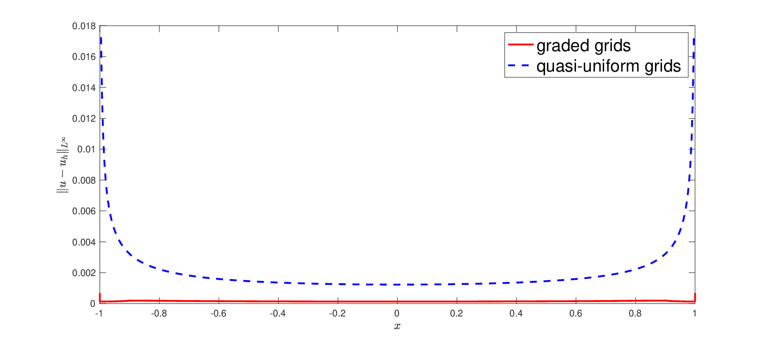
To achieve the optimal convergence rates, several key ideas are introduced and utilized in this paper. First, we show the relationship between high-order Hölder constant of solution and distance to boundary, which indicates that the scale of Ωi\Omega_{i}, denoted by HiH_{i}, should also depend on dist⁡(xi,∂Ω)\mathrm{dist}(x_{i},\partial\Omega). Second, upon the ratio between dist⁡(xi,∂Ω)\mathrm{dist}(x_{i},\partial\Omega) and local grid size, we introduce the δ\delta-interior nodes in (24) where the consistency can be proved. This, together with a discrete barrier function and the discrete comparison principle, leads to the optimal error estimates. The analysis only requires the local quasi-uniformity hence can be applied to both quasi-uniform and graded grids. Moreover, the analysis only requires the minimal Hölder regularity of the data, and interestingly, the Hölder regularity indeed influences the optimal scale of Ωi\Omega_{i}, see Theorem 24 and Theorem 26.

It is interesting to note that, there is a strong connection between our work and the monotone two-scale methods for solving Monge-Ampère equations [25]. We note that the two-scale methods are also important for problems in which preserving monotonicity and comparison is of relevance [24, 21]. In our work, the scale of Ωi\Omega_{i} can be viewed as the second scale in addition to grid size, which depends on the distance to boundary due to the PDE theory of (1). Moreover, it is known that monotonicity is one of the essential ingredients in devising convergent schemes for fully nonlinear PDEs [5]. Our work, in this sense, is expected to have broad prospects in solving nonlinear problems involving integral fractional Laplacian.

The rest of the paper is organized as follows. In Section 2, we review the regularity results for the integral fractional Laplace equation (1). In Section 3, we introduce a monotone discretization and prove the discrete comparison principle. The consistency error is divided into singular and tail parts, which are estimated in Section 4 and Section 5 separately. In Section 6, combining the discrete comparison principle and the consistency error, we establish the pointwise error estimates for the numerical scheme. Finally, in Section 7, several numerical examples are exhibited to illustrate the theoretical results.

2 Preliminary results

In this section, we present some preliminary results in the analysis setting. For β>0\beta>0, we denote by |⋅|Cβ​(U)|\cdot|_{C^{\beta}(U)} the Cβ​(U)C^{\beta}(U) seminorm. More precisely, we will write β=k+β′\beta=k+\beta^{\prime} with kk integer and β′∈(0,1]\beta^{\prime}\in(0,1], then

|w|Cβ​(U)=|w|Ck,β′​(U)\displaystyle|w|_{C^{\beta}(U)}=|w|_{C^{k,\beta^{\prime}}(U)} :=supx,y∈U,x≠y|Dk​w​(x)−Dk​w​(y)||x−y|β′,\displaystyle:=\sup_{x,y\in U,x\neq y}\frac{|D^{k}w(x)-D^{k}w(y)|}{|x-y|^{\beta^{\prime}}},
‖w‖Cβ​(U)\displaystyle\|w\|_{C^{\beta}(U)} :=∑ℓ=0k(supx∈U|Dℓ​w​(x)|)+|w|Cβ​(U).\displaystyle:=\sum_{\ell=0}^{k}\left(\sup_{x\in U}|D^{\ell}w(x)|\right)+|w|_{C^{\beta}(U)}.

Next, we summarize the Hölder regularity results for (1) given in [29]. To begin with, we state the definition of Lipschitz domain (cf. [19, Definition 1.2.1.1]).

Definition 1 (Lipschitz domain).

Let Ω\Omega be an open subset of ℝn\mathbb{R}^{n}. We say that Ω\Omega is a Lipschitz domain if for every x∈∂Ωx\in\partial\Omega there exists a neighborhood VV of xx in ℝn\mathbb{R}^{n} and new orthogonal coordinates {z1,⋯,zn}\{z_{1},\cdots,z_{n}\} such that

  • (a)

    VV is an hypercube in the new coordinates:

    V={(z1,⋯,zn):−aj<zj<aj,1≤j≤n};V=\{(z_{1},\cdots,z_{n}):-a_{j}<z_{j}<a_{j},~1\leq j\leq n\};
  • (b)

    there exists a Lipschitz function φ\varphi, defined in

    V′:={(z1,⋯,zn−1):−aj<zj<aj, 1≤j≤n−1}V^{\prime}:=\{(z_{1},\cdots,z_{n-1}):-a_{j}<z_{j}<a_{j},\;1\leq j\leq n-1\}

    and such that

    |φ⁡(z′)|≤an/2​ for every ​z′=(z1,⋯,zn−1)∈V′,\displaystyle|\varphi(z^{\prime})|\leq a_{n}/2\text{ for every }z^{\prime}=(z_{1},\cdots,z_{n-1})\in V^{\prime},
    Ω∩V={z=(z′,zn)∈V:zn<φ⁡(z′)},\displaystyle\Omega\cap V=\{z=(z^{\prime},z_{n})\in V:z_{n}<\varphi(z^{\prime})\},
    ∂Ω∩V={z=(z′,zn)∈V:zn=φ⁡(z′)}.\displaystyle\partial\Omega\cap V=\{z=(z^{\prime},z_{n})\in V:z_{n}=\varphi(z^{\prime})\}.

Proposition 2 (Proposition 1.1 in [29]).

Let Ω\Omega be a bounded Lipschitz domain satisfying exterior ball condition, f∈L∞​(Ω)f\in L^{\infty}(\Omega), and uu be a solution of (1). Then u∈Cs​(ℝn)u\in C^{s}(\mathbb{R}^{n}) and

‖u‖Cs​(ℝn)≤C​‖f‖L∞​(Ω),\|u\|_{C^{s}(\mathbb{R}^{n})}\leq C\|f\|_{L^{\infty}(\Omega)},

where CC is a constant depending only on Ω\Omega and ss.

Moreover, the higher-order Hölder regularity inside Ω\Omega can be obtained when ff is Hölder continuous, which hinges on the weighted norm up to the boundary. Let δ⁡(x)\delta(x) be the distance to the boundary of xx, and δ⁡(x,y):=min⁡{δ⁡(x),δ⁡(y)}\delta(x,y):=\min\{\delta(x),\delta(y)\}. Following [29], let β>0\beta>0 and σ≥−β\sigma\geq-\beta, we define the seminorm

|w|β;U(σ):=supx,y∈U(δ​(x,y)β+σ​|Dk​w​(x)−Dk​w​(y)||x−y|β′)∀w∈Cβ​(U):=Ck,β′​(U).|w|_{\beta;U}^{(\sigma)}:=\sup_{x,y\in U}\left(\delta(x,y)^{\beta+\sigma}\frac{|D^{k}w(x)-D^{k}w(y)|}{|x-y|^{\beta^{\prime}}}\right)\quad\forall w\in C^{\beta}(U):=C^{k,\beta^{\prime}}(U). (3)

For σ>−1\sigma>-1, the associated norm ∥⋅∥β;U(σ)\|\cdot\|_{\beta;U}^{(\sigma)} is defined as follows:

  1. 1.

    For σ≥0\sigma\geq 0,

    ‖w‖β;U(σ):=∑ℓ=0ksupx∈U(δ​(x)ℓ+σ​|Dℓ​w​(x)|)+|w|β;U(σ);\|w\|_{\beta;U}^{(\sigma)}:=\sum_{\ell=0}^{k}\sup_{x\in U}\left(\delta(x)^{\ell+\sigma}|D^{\ell}w(x)|\right)+|w|_{\beta;U}^{(\sigma)}; (4a)
  2. 2.

    For 0>σ>−10>\sigma>-1,

    ‖w‖β;U(σ):=‖w‖C−σ​(U)+∑ℓ=1ksupx∈U(δ​(x)ℓ+σ​|Dℓ​w​(x)|)+|w|β;U(σ).\|w\|_{\beta;U}^{(\sigma)}:=\|w\|_{C^{-\sigma}(U)}+\sum_{\ell=1}^{k}\sup_{x\in U}\left(\delta(x)^{\ell+\sigma}|D^{\ell}w(x)|\right)+|w|_{\beta;U}^{(\sigma)}. (4b)

The following result is the starting point of this work.

Proposition 3 (Proposition 1.4 in [29]).

Let Ω\Omega be a bounded domain, and β>0\beta>0 be such that neither β\beta nor β+2​s\beta+2s is an integer. Let f∈Cβ​(Ω)f\in C^{\beta}(\Omega) be such that ‖f‖β;Ω(s)<∞\|f\|_{\beta;\Omega}^{(s)}<\infty, and u∈Cs​(ℝn)u\in C^{s}(\mathbb{R}^{n}) be a solution of (1). Then, u∈Cβ+2​s​(Ω)u\in C^{\beta+2s}(\Omega) and

‖u‖β+2​s;Ω(−s)≤C⁡(‖u‖Cs​(ℝn)+‖f‖β;Ω(s)),\|u\|_{\beta+2s;\Omega}^{(-s)}\leq C(\|u\|_{C^{s}(\mathbb{R}^{n})}+\|f\|_{\beta;\Omega}^{(s)}), (5)

where CC is a constant depending only on Ω\Omega, ss and β\beta.

Remark 4 (blow-up behavior).

We further note that the blow-up behavior of the constant CC in (5) is |β−m|−1|\beta-m|^{-1} or |β+2​s−m|−1|\beta+2s-m|^{-1} as β\beta or β+2​s\beta+2s approaching to some integer mm, which can be found in the proof of [30, Proposition 2.5 & Proposition 2.7].

As a corollary, the dependence of the δ⁡(x)\delta(x) on the Hölder norm of uu is given as follows. For the sake of expository simplicity, we adopt β\beta as the Hölder index of uu. We also assume Ω\Omega to be a bounded Lipschitz domain with exterior ball condition in what follows.

Corollary 5 (δ\delta-dependence in Hölder norm).

Let Ω\Omega be a bounded Lipschitz domain with exterior ball condition, and β>2​s\beta>2s be such that neither β−2​s\beta-2s nor β\beta is an integer. Let f∈L∞​(Ω)f\in L^{\infty}(\Omega) be such that ‖f‖β−2​s;Ω(s)<∞\|f\|_{\beta-2s;\Omega}^{(s)}<\infty. Then, u∈Cβ​(Ω)u\in C^{\beta}(\Omega) and

∥u∥Cβ​({x∈Ω:δ⁡(x)≥ρ})≤Cρs−β∀ρ∈(0,diam(Ω)],\|u\|_{C^{\beta}(\{x\in\Omega:~\delta(x)\geq\rho\})}\leq C\rho^{s-\beta}\quad\forall\rho\in(0,\mathrm{diam}(\Omega)], (6)

where CC is a constant depending only on Ω\Omega, ss, β\beta, ‖f‖L∞​(Ω)\|f\|_{L^{\infty}(\Omega)} and ‖f‖β−2​s;Ω(s)\|f\|_{\beta-2s;\Omega}^{(s)}.

Proof.

We denote Uρ:={x∈Ω:δ⁡(x)≥ρ}U_{\rho}:=\{x\in\Omega:~\delta(x)\geq\rho\}. Using Proposition 3 and the definition of weighted seminorm (3), we have

|u|Cβ​(Uρ)\displaystyle|u|_{C^{\beta}(U_{\rho})} =ρs−β​supx,y∈Uρρβ−s​|Dk​u​(x)−Dk​u​(y)||x−y|β′\displaystyle=\rho^{s-\beta}\sup_{x,y\in U_{\rho}}\rho^{\beta-s}\frac{|D^{k}u(x)-D^{k}u(y)|}{|x-y|^{\beta^{\prime}}}
≤ρs−βsupx,y∈Uρδ(x,y)β−s|Dk​u​(x)−Dk​u​(y)||x−y|β′(since β>s)\displaystyle\leq\rho^{s-\beta}\sup_{x,y\in U_{\rho}}\delta(x,y)^{\beta-s}\frac{|D^{k}u(x)-D^{k}u(y)|}{|x-y|^{\beta^{\prime}}}\quad(\text{since }\beta>s)
≤ρs−β​|u|β;Uρ(−s)≤C⁡(Ω,s,β)​ρs−β​(‖u‖Cs​(ℝn)+‖f‖β−2​s;Ω(s))\displaystyle\leq\rho^{s-\beta}|u|_{\beta;U_{\rho}}^{(-s)}\leq C(\Omega,s,\beta)\rho^{s-\beta}(\|u\|_{C^{s}(\mathbb{R}^{n})}+\|f\|_{\beta-2s;\Omega}^{(s)})
≤C⁡(Ω,s,β,‖f‖L∞​(Ω),‖f‖β−2​s;Ω(s))​ρs−β.\displaystyle\leq C(\Omega,s,\beta,\|f\|_{L^{\infty}(\Omega)},\|f\|_{\beta-2s;\Omega}^{(s)})\rho^{s-\beta}.

Here, we use Proposition 2 in the last step. Similarly, for any 1≤ℓ≤k<β1\leq\ell\leq k<\beta,

supx∈Uρ|Dℓ​u​(x)|≤ρs−ℓ​‖u‖β;Uρ(−s)≤C⁡(Ω,s,β,‖f‖L∞​(Ω),‖f‖β−2​s;Ω(s))​ρs−β,\sup_{x\in U_{\rho}}|D^{\ell}u(x)|\leq\rho^{s-\ell}\|u\|_{\beta;U_{\rho}}^{(-s)}\leq C(\Omega,s,\beta,\|f\|_{L^{\infty}(\Omega)},\|f\|_{\beta-2s;\Omega}^{(s)})\rho^{s-\beta},

where we use ρβ−ℓ≤diam​(Ω)β−ℓ\rho^{\beta-\ell}\leq\mathrm{diam}(\Omega)^{\beta-\ell} in the last step. This completes the proof.

At this point, we recall a useful estimate corresponding to the integrability of kernel outside the domain (cf. [19, Eq. (1,3,2,12)]): There exist two constants 0<C1≤C20<C_{1}\leq C_{2} such that

C1​(Ω,s)​δ​(x)−2​s≤∫Ωc1|x−y|n+2​s​𝑑y≤C2​(Ω,s)​δ​(x)−2​s.C_{1}(\Omega,s)\delta(x)^{-2s}\leq\int_{\Omega^{c}}\frac{1}{|x-y|^{n+2s}}\,\mathrm{d}y\leq C_{2}(\Omega,s)\delta(x)^{-2s}. (7)

In the last of this section, we present an elementary result of the center difference in Hölder seminorm along the direction θ∈Sn−1\theta\in S^{n-1}, where Sn−1S^{n-1} denotes the unit (n−1)(n-1)-sphere.

Lemma 6 (FD in Hölder seminorm).

Let ρ>0\rho>0 and u∈Cβ​(Bρ​(x))u\in C^{\beta}(B_{\rho}(x)).

  1. 1.

    If β≤2\beta\leq 2, then there exists C>0C>0 for any θ∈Sn−1\theta\in S^{n-1},

    |2​u​(x)−u⁡(x+ρ​θ)−u⁡(x−ρ​θ)|≤C​ρβ​|u|Cβ​(Bρ​(x)).|2u(x)-u(x+\rho\theta)-u(x-\rho\theta)|\leq C\rho^{\beta}|u|_{C^{\beta}(B_{\rho}(x))}.
  2. 2.

    If 2<β≤42<\beta\leq 4, then there exists C>0C>0 for any θ∈Sn−1\theta\in S^{n-1},

    |2​u​(x)−u⁡(x+ρ​θ)−u⁡(x−ρ​θ)+ρ2​∂2u∂θ2​(x)|≤C​ρβ​|u|Cβ​(Bρ​(x)).\left|2u(x)-u(x+\rho\theta)-u(x-\rho\theta)+\rho^{2}\frac{\partial^{2}u}{\partial\theta^{2}}(x)\right|\leq C\rho^{\beta}|u|_{C^{\beta}(B_{\rho}(x))}.

Proof.

Recall that β=k+β′\beta=k+\beta^{\prime} for integer k≤3k\leq 3 and β′∈(0,1]\beta^{\prime}\in(0,1], we have by Taylor’s expansion with Lagrange remainder term that, for some ξ∈Bρ​(x)\xi\in B_{\rho}(x),

u⁡(x+ρ​θ)\displaystyle u(x+\rho\theta) =u⁡(x)+∑j=1k−11j!​∂ju∂θj​(x)​ρj+1k!​∂ku∂θk​(ξ)​ρk\displaystyle=u(x)+\sum_{j=1}^{k-1}\frac{1}{j!}\frac{\partial^{j}u}{\partial\theta^{j}}(x)\rho^{j}+\frac{1}{k!}\frac{\partial^{k}u}{\partial\theta^{k}}(\xi)\rho^{k}
=u⁡(x)+∑j=1k1j!​∂ju∂θj​(x)​ρj+1k!​(∂ku∂θk​(ξ)−∂ku∂θk​(x))​ρk.\displaystyle=u(x)+\sum_{j=1}^{k}\frac{1}{j!}\frac{\partial^{j}u}{\partial\theta^{j}}(x)\rho^{j}+\frac{1}{k!}\left(\frac{\partial^{k}u}{\partial\theta^{k}}(\xi)-\frac{\partial^{k}u}{\partial\theta^{k}}(x)\right)\rho^{k}.

The last term can be controlled by using the definition of Hölder seminorm, which completes the proof.

3 Monotone discretization

For ease of discretization and the sake of simplicity of the exposition, we shall henceforth consider Ω\Omega to be a bounded open polytope. We assume Ω\Omega admits an admissible triangulation 𝒯h\mathcal{T}_{h}, i.e., ∪T∈𝒯hT¯=Ω¯\cup_{T\in\mathcal{T}_{h}}\bar{T}=\overline{\Omega}. Let 𝒩h\mathcal{N}_{h} denote the node set of 𝒯h\mathcal{T}_{h}, 𝒩hb:={xi∈𝒩h:xi∈∂Ω}\mathcal{N}_{h}^{b}:=\{x_{i}\in\mathcal{N}_{h}:x_{i}\in\partial\Omega\} be the collection of boundary nodes, and 𝒩h0:=𝒩h∖𝒩hb\mathcal{N}_{h}^{0}:=\mathcal{N}_{h}\setminus\mathcal{N}_{h}^{b}. We require that the family of triangulation under consideration satisfies shape regularity and local quasi-uniformity. Note that the latter can be deduced by the former when n≥2n\geq 2 [12]. More precisely, let hTh_{T} and ρT\rho_{T} respectively be the diameter of TT and diameter of the largest ball contained in TT, the conditions of triangulation read

∃λ1>0\displaystyle\exists\lambda_{1}>0~ s.t. ​hT≤λ1​ρT​∀T∈𝒯h,\displaystyle~\mbox{s.t. }h_{T}\leq\lambda_{1}\rho_{T}~\forall T\in\mathcal{T}_{h}, (8a)
∃λ2>0\displaystyle\exists\lambda_{2}>0~ s.t. ​hT≤λ2​hT′​∀T,T′∈𝒯h​ with ​T¯∩T¯′≠∅.\displaystyle~\mbox{s.t. }h_{T}\leq\lambda_{2}h_{T^{\prime}}~\forall T,T^{\prime}\in\mathcal{T}_{h}\mbox{ with }\bar{T}\cap\bar{T}^{\prime}\neq\varnothing. (8b)

For each xi∈𝒩h0x_{i}\in\mathcal{N}_{h}^{0}, we define ωi=∪T¯∋xiT¯\omega_{i}=\cup_{\bar{T}\ni x_{i}}\bar{T}, and denote by hih_{i} the radius of inscribed sphere centered at xix_{i} for ωi\omega_{i}. Clearly, for any T¯∋xi\bar{T}\ni x_{i},

2​λ1​λ2⏟:=λhi≥λ1λ2ρT≥λ2hT≥maxT′¯∋xihT′.\underbrace{2\lambda_{1}\lambda_{2}}_{:=\lambda}h_{i}\geq\lambda_{1}\lambda_{2}\rho_{T}\geq\lambda_{2}h_{T}\geq\max_{\bar{T^{\prime}}\ni x_{i}}h_{T^{\prime}}. (9)

Let 𝕍h\mathbb{V}_{h} be the space of continuous piecewise linear functions over 𝒯h\mathcal{T}_{h} that vanish in Ωc\Omega^{c}, that is,

𝕍h:={v:v|T∈𝒫1(T)∀T∈𝒯h,v|Ωc=0}.\mathbb{V}_{h}:=\{v:\;v|_{T}\in\mathcal{P}_{1}(T)~\forall T\in\mathcal{T}_{h},\;v|_{\Omega^{c}}=0\}. (10)

Following [20], we divide the integral of fractional Laplacian into two parts: The singular part and the tail part.

3.1 Discretization of singular integral

For each xi∈𝒩h0x_{i}\in\mathcal{N}_{h}^{0}, we take a proper scale HiH_{i} such that BHi​(xi)⊂ΩB_{H_{i}}(x_{i})\subset\Omega. The standard centered difference of the Δ​u​(xi)\Delta u(x_{i}) with spacing HiH_{i} is denoted by

ΔFD​u​(xi,Hi)Hi2:=∑j=1nu⁡(xi+Hi​ej)−2​u​(xi)+u⁡(xi−Hi​ej)Hi2,\frac{\Delta_{\rm FD}u(x_{i};H_{i})}{H_{i}^{2}}:=\sum_{j=1}^{n}\frac{u(x_{i}+H_{i}e_{j})-2u(x_{i})+u(x_{i}-H_{i}e_{j})}{H_{i}^{2}},

where eje_{j} is the unit vector of the jj-th coordinate.

For the discretization of singular integral, we consider a star-shaped domain Ωi\Omega_{i} centered at xix_{i}, i.e., by using the multi-dimensional polar coordinate

Ωi:={xi+ρθ:θ∈Sn−1,ρ∈[0,ρi(θ)),ρi(θ)>0}.\Omega_{i}:=\{x_{i}+\rho\theta:\theta\in S^{n-1},\rho\in[0,\rho_{i}(\theta)),\rho_{i}(\theta)>0\}. (11)

The domain Ωi\Omega_{i} is assumed to satisfy the following conditions:

  1. 1.

    Interior of Ω\Omega: Ωi⊂Ω\Omega_{i}\subset\Omega, ∀xi∈𝒩h0\forall x_{i}\in\mathcal{N}_{h}^{0}.

  2. 2.

    Symmetry:

    xi+(z1,⋯,zn)∈Ωi\displaystyle x_{i}+(z_{1},\cdots,z_{n})\in\Omega_{i} (12)
    ⟺\displaystyle\Longleftrightarrow xi+(±zσ⁡(1),⋯,±zσ⁡(n))∈Ωi​ for any permutation ​σ.\displaystyle x_{i}+(\pm z_{\sigma(1)},\cdots,\pm z_{\sigma(n)})\in\Omega_{i}\mbox{ for any permutation }\sigma.
  3. 3.

    Quasi-uniformity: there exist positive constants c¯S,c¯S\underline{c}_{S},\bar{c}_{S}, such that

    c¯S​Hi≤ρi​(θ)≤c¯S​Hi∀xi∈𝒩h0,θ∈Sn−1.\underline{c}_{S}H_{i}\leq\rho_{i}(\theta)\leq\bar{c}_{S}H_{i}\quad\forall x_{i}\in\mathcal{N}_{h}^{0},\theta\in S^{n-1}. (13)

Using the symmetry of Ωi\Omega_{i} and polar coordinate transformation y↦xi+z=xi+ρ​θy\mapsto x_{i}+z=x_{i}+\rho\theta which satisfies d​z=ρn−1​d​ρ​d​Sθ\mathrm{d}z=\rho^{n-1}\mathrm{d}\rho\mathrm{d}S_{\theta}, we have

∫Ωiv⁡(xi)−v⁡(y)|xi−y|n+2​s​𝑑y\displaystyle\int_{\Omega_{i}}\frac{v(x_{i})-v(y)}{|x_{i}-y|^{n+2s}}\,\mathrm{d}y =12​∫Ωi−xi2​v​(xi)−v⁡(xi+z)−v⁡(xi−z)|z|n+2​s​𝑑z\displaystyle=\frac{1}{2}\int_{\Omega_{i}-x_{i}}\frac{2v(x_{i})-v(x_{i}+z)-v(x_{i}-z)}{|z|^{n+2s}}\,\mathrm{d}z (14)
=12​∫Sn−1∫0ρi​(θ)2​v​(xi)−v⁡(xi+ρ​θ)−v⁡(xi−ρ​θ)ρ1+2​s​dρ​d​Sθ.\displaystyle=\frac{1}{2}{\color[rgb]{0,0,0}\int_{S^{n-1}}\int_{0}^{\rho_{i}(\theta)}}\frac{2v(x_{i})-v(x_{i}+\rho\theta)-v(x_{i}-\rho\theta)}{\rho^{1+2s}}\,{\color[rgb]{0,0,0}\mathrm{d}\rho}\mathrm{d}S_{\theta}.

Suppose the function v∈C2​(Ωi)v\in C^{2}(\Omega_{i}), the above integral can be approximated by the following second-order differential operator

12​∫Sn−1∫0ρi​(θ)2​v​(xi)−v⁡(xi+ρ​θ)−v⁡(xi−ρ​θ)ρ1+2​s​𝑑ρ​d​Sθ\displaystyle\frac{1}{2}{\color[rgb]{0,0,0}\int_{S^{n-1}}\int_{0}^{\rho_{i}(\theta)}}\,\frac{2v(x_{i})-v(x_{i}+\rho\theta)-v(x_{i}-\rho\theta)}{\rho^{1+2s}}\,{\color[rgb]{0,0,0}\mathrm{d}\rho}\mathrm{d}S_{\theta}
≈\displaystyle\approx −12​D2​u​(xi):∫Sn−1∫0ρi​(θ)ρ1−2​s​𝑑ρ​θ⊗θ​d​Sθ\displaystyle-\frac{1}{2}D^{2}u(x_{i}):{\color[rgb]{0,0,0}\int_{S^{n-1}}\int_{0}^{\rho_{i}(\theta)}\rho^{1-2s}\mathrm{d}\rho\;\theta\otimes\theta\,\mathrm{d}S_{\theta}}
=\displaystyle= −Hi2−2​s4​(1−s)​D2​u​(xi):∫Sn−1(ρi​(θ)Hi)2−2​s​θ⊗θ​d​Sθ.\displaystyle-\frac{H_{i}^{2-2s}}{4(1-s)}D^{2}u(x_{i}):\int_{S^{n-1}}\left(\frac{\rho_{i}(\theta)}{H_{i}}\right)^{2-2s}\theta\otimes\theta\,\mathrm{d}S_{\theta}.

Thanks to the symmetry of Ωi\Omega_{i}, the last integral can be simplified by the lemma below.

Lemma 7 (symmetric integral).

Under the conditions (12) – (13),

14​(1−s)∫Sn−1(ρi​(θ)Hi)2−2​sθ⊗θdSθ=14​n​(1−s)​∫Sn−1(ρi​(θ)Hi)2−2​s​d​Sθ⏟:=κn,s,iIn,\frac{1}{4(1-s)}\int_{S^{n-1}}\left(\frac{\rho_{i}(\theta)}{H_{i}}\right)^{2-2s}\theta\otimes\theta\,\mathrm{d}S_{\theta}=\underbrace{\frac{1}{4n(1-s)}\int_{S^{n-1}}\left(\frac{\rho_{i}(\theta)}{H_{i}}\right)^{2-2s}\,\mathrm{d}S_{\theta}}_{:=\kappa_{n,s,i}}I_{n}, (15)

where InI_{n} is the identity matrix. Moreover, κn,s,i\kappa_{n,s,i} is a uniformly bounded constant.

Proof.

It is readily seen that ρi​(±θσ⁡(1),⋯,±θσ⁡(n))\rho_{i}(\pm\theta_{\sigma(1)},\cdots,\pm\theta_{\sigma(n)}) are the same. For any fixed permutation σ\sigma, let θj1,⋯,jnσ:=((−1)j1​θσ⁡(1),⋯,(−1)jn​θσ⁡(n))\theta_{j_{1},\cdots,j_{n}}^{\sigma}:=((-1)^{j_{1}}\theta_{\sigma(1)},\cdots,(-1)^{j_{n}}\theta_{\sigma(n)}), then

∑j1,⋯,jn=01θj1,⋯,jnσ⊗θj1,⋯,jnσ=2n​diag​(θσ⁡(1)2,⋯,θσ⁡(n)2),\sum_{j_{1},\cdots,j_{n}=0}^{1}\theta_{j_{1},\cdots,j_{n}}^{\sigma}\otimes\theta_{j_{1},\cdots,j_{n}}^{\sigma}=2^{n}\mathrm{diag}(\theta^{{\color[rgb]{0,0,0}2}}_{\sigma(1)},\cdots,\theta^{{\color[rgb]{0,0,0}2}}_{\sigma(n)}),

which together with θj1,⋯,jnσ∈Sn−1\theta_{j_{1},\cdots,j_{n}}^{\sigma}\in S^{n-1} yields

∑σ∑j1,⋯,jn=01θj1,⋯,jnσ⊗θj1,⋯,jnσ=2n​n!n​In.\sum_{\sigma}\sum_{j_{1},\cdots,j_{n}=0}^{1}\theta_{j_{1},\cdots,j_{n}}^{\sigma}\otimes\theta_{j_{1},\cdots,j_{n}}^{\sigma}=\frac{2^{n}n!}{n}I_{n}.

Hence, the contribution of θ⊗θ\theta\otimes\theta in the integral is identically to 1n​In\frac{1}{n}I_{n}, which leads to (15). The quasi-uniformity (13) implies that κn,s,i=𝒪⁡(1)\kappa_{n,s,i}=\mathcal{O}(1).

Combining (14) – (15), the discretization of the singular integral is defined by

ℒhS​[u]​(xi)\displaystyle\mathcal{L}_{h}^{S}[u](x_{i}) :=−κn,s,i​ΔFD​u​(xi,Hi)Hi2​s\displaystyle:=-\kappa_{n,s,i}\frac{\Delta_{\rm FD}u(x_{i};H_{i})}{H_{i}^{2s}} (16)
=−κn,s,i∑j=1nu⁡(xi+Hi​ej)−2​u​(xi)+u⁡(xi−Hi​ej)Hi2​s.\displaystyle=-\kappa_{n,s,i}\sum_{j=1}^{n}\frac{u(x_{i}+H_{i}e_{j})-2u(x_{i})+u(x_{i}-H_{i}e_{j})}{H_{i}^{2s}}.
Remark 8 (dependence of HiH_{i}).

So far the discretization of singular integral depends solely on Ωi\Omega_{i} with scale HiH_{i}. We will show below that the HiH_{i} should depend on local grid size and the distance of xix_{i} to the boundary. Therefore, for the sake of consistency, we adopt ℒhS\mathcal{L}_{h}^{S} to indicate the essential dependence on hh.

Remark 9 (examples of Ωi\Omega_{i}).

The simplest example that satisfies the condition (12) – (13) is Ωi=BHi​(xi)\Omega_{i}=B_{H_{i}}(x_{i}), which gives κn,s,i=|Sn−1|4​n​(1−s)=ωn4​(1−s)\kappa_{n,s,i}=\frac{|S^{n-1}|}{4n(1-s)}=\frac{\omega_{n}}{4(1-s)}, where ωn=2​πn/2n​Γ​(n/2)\omega_{n}=\frac{2\pi^{n/2}}{n\Gamma(n/2)} is the volume of unit ball in ℝn\mathbb{R}^{n}. Another example is the nn-dimensional cube centered at xix_{i} with scale Hi/nH_{i}/\sqrt{n}, namely

Ωi={xi+(z1,⋯,zn):|zi|<Hin}.\Omega_{i}=\{x_{i}+(z_{1},\cdots,z_{n})~:~|z_{i}|<\frac{H_{i}}{\sqrt{n}}\}.

Clearly, Ωi⊂BHi​(xi)⊂Ω\Omega_{i}\subset B_{H_{i}}(x_{i})\subset\Omega. A direct calculation shows that in 2D,

κn,s,i\displaystyle\kappa_{n,s,i} =11−s​∫0π/4(12​cos⁡θ)2−2​s​𝑑θ\displaystyle=\frac{1}{1-s}\int_{0}^{\pi/4}\left(\frac{1}{\sqrt{2}\cos\theta}\right)^{2-2s}\,\mathrm{d}\theta (17)
={1(1−s)​22−s​[π​Γ​(s−12)Γ⁡(s)−B12​(s−12,12)]s≠0.5,1(1−s)​2−s​tanh−1⁡(tan⁡(π8))s=0.5.\displaystyle=\left\{\begin{array}[]{ll}\frac{1}{(1-s)2^{2-s}}\left[\frac{\sqrt{\pi}\Gamma(s-\frac{1}{2})}{\Gamma(s)}-B_{\frac{1}{2}}(s-\frac{1}{2},\frac{1}{2})\right]&\quad s\neq 0.5,\\ \frac{1}{(1-s)2^{-s}}\tanh^{-1}\left(\tan(\frac{\pi}{8})\right)&\quad s=0.5.\end{array}\right.

Here, Bx​(a,b)B_{x}(a,b) is the incomplete beta function.

3.2 Monotonicity

We seek uh∈𝕍hu_{h}\in\mathbb{V}_{h} such that for xi∈𝒩h0x_{i}\in\mathcal{N}_{h}^{0},

ℒh[uh](xi):=−κn,s,i​ΔF​D​uh​(xi,Hi)Hi2​s⏟ℒhS​[uh]​(xi)+∫Ωicuh​(xi)−uh​(y)|xi−y|n+2​s​dy⏟:=ℒhT​[uh]​(xi)=f(xi).\mathcal{L}_{h}[u_{h}](x_{i}):=\underbrace{-\kappa_{n,s,i}\frac{\Delta_{FD}u_{h}(x_{i};H_{i})}{H_{i}^{2s}}}_{\mathcal{L}_{h}^{S}[u_{h}](x_{i})}+\underbrace{\int_{\Omega_{i}^{c}}\frac{u_{h}(x_{i})-u_{h}(y)}{|x_{i}-y|^{n+2s}}\,\mathrm{d}y}_{:=\mathcal{L}_{h}^{T}[u_{h}](x_{i})}=f(x_{i}). (18)

A similar definition was first proposed by Huang and Oberman [20] on 1D uniform grids with Hi=hH_{i}=h. Any function in 𝕍h\mathbb{V}_{h} has a pointwise definition and hence ℒh\mathcal{L}_{h} is well defined. The tail of integral ℒhT​[uh]\mathcal{L}_{h}^{T}[u_{h}] renders integral of piecewise linear functions outside Ωi\Omega_{i}.

We now show that (18) is monotone and prove the discrete comparison principle.

Lemma 10 (monotonicity).

Let vh,wh∈𝕍hv_{h},w_{h}\in\mathbb{V}_{h}. If vh−whv_{h}-w_{h} attains a non-negative maximum at an interior node xi∈𝒩h0x_{i}\in\mathcal{N}_{h}^{0}, then ℒh​[vh]​(xi)≥ℒh​[wh]​(xi)\mathcal{L}_{h}[v_{h}](x_{i})\geq\mathcal{L}_{h}[w_{h}](x_{i}).

Proof.

If vh−whv_{h}-w_{h} attains a non-negative maximum at xi∈𝒩h0x_{i}\in\mathcal{N}_{h}^{0}, then vh​(xi)≥wh​(xi)v_{h}(x_{i})\geq w_{h}(x_{i}), and

vh​(xi)−vh​(y)≥wh​(xi)−wh​(y)∀y∈Ω.v_{h}(x_{i})-v_{h}(y)\geq w_{h}(x_{i})-w_{h}(y)\quad\forall y\in\Omega.

Then, we have

ℒhS​[vh]​(xi)=−κn,s,i​ΔF​D​vh​(xi,Hi)Hi2​s\displaystyle\mathcal{L}_{h}^{S}[v_{h}](x_{i})=-\kappa_{n,s,i}\frac{\Delta_{FD}v_{h}(x_{i};H_{i})}{H_{i}^{2s}} ≥−κn,s,i​ΔF​D​wh​(xi,Hi)Hi2​s=ℒhS​[wh]​(xi),\displaystyle\geq-\kappa_{n,s,i}\frac{\Delta_{FD}w_{h}(x_{i};H_{i})}{H_{i}^{2s}}=\mathcal{L}_{h}^{S}[w_{h}](x_{i}),
ℒhT​[vh]​(xi)=∫ℝn∖Ωivh​(xi)−vh​(y)|xi−y|n+2​s​𝑑y\displaystyle\mathcal{L}_{h}^{T}[v_{h}](x_{i})=\int_{\mathbb{R}^{n}\setminus\Omega_{i}}\frac{v_{h}(x_{i})-v_{h}(y)}{|x_{i}-y|^{n+2s}}\mathrm{d}y ≥∫ℝn∖Ωiwh​(xi)−wh​(y)|xi−y|n+2​s​dy=ℒhT​[wh]​(xi),\displaystyle\geq\int_{\mathbb{R}^{n}\setminus\Omega_{i}}\frac{w_{h}(x_{i})-w_{h}(y)}{|x_{i}-y|^{n+2s}}\mathrm{d}y=\mathcal{L}_{h}^{T}[w_{h}](x_{i}),

which implies ℒh​[vh]​(xi)≥ℒh​[wh]​(xi)\mathcal{L}_{h}[v_{h}](x_{i})\geq\mathcal{L}_{h}[w_{h}](x_{i}), as asserted.

Lemma 11 (discrete barrier function).

Let bh∈𝕍hb_{h}\in\mathbb{V}_{h} satisfy

bh​(xi):=1∀xi∈𝒩h0.\displaystyle b_{h}(x_{i}):=1\quad\forall x_{i}\in\mathcal{N}_{h}^{0}. (19)

Denoting δi\delta_{i} as the shorthand of δ⁡(xi)\delta(x_{i}), then we have

ℒh​[bh]​(xi)≥C​δi−2​s∀xi∈𝒩h0,\mathcal{L}_{h}[b_{h}](x_{i})\geq C\delta_{i}^{-2s}\quad\forall x_{i}\in\mathcal{N}_{h}^{0}, (20)

where the constant CC depends only on ss and Ω\Omega.

Proof.

Since ℒhS​[bh]≥0\mathcal{L}_{h}^{S}[b_{h}]\geq 0, it suffices to prove ℒhT​[bh]​(xi)≥C​δi−2​s\mathcal{L}_{h}^{T}[b_{h}](x_{i})\geq C\delta_{i}^{-2s}. By the definition of bhb_{h},

ℒhT​[bh]​(xi)\displaystyle\mathcal{L}_{h}^{T}[b_{h}](x_{i}) =∫ℝn∖Ωibh​(xi)−bh​(y)|xi−y|n+2​s​𝑑y≥∫Ωcbh​(xi)−bh​(y)|xi−y|n+2​s​𝑑y\displaystyle=\int_{\mathbb{R}^{n}\setminus\Omega_{i}}\frac{b_{h}(x_{i})-b_{h}(y)}{|x_{i}-y|^{n+2s}}\mathrm{d}y\geq\int_{\Omega^{c}}\frac{b_{h}(x_{i})-b_{h}(y)}{|x_{i}-y|^{n+2s}}\mathrm{d}y
=∫Ωc1|xi−y|n+2​s​dy≥C​δi−2​s,\displaystyle=\int_{\Omega^{c}}\frac{1}{|x_{i}-y|^{n+2s}}\mathrm{d}y\geq C\delta_{i}^{-2s},

where (7) is used in the last step.

Lemma 12 (discrete comparison principle).

Let vh,wh∈𝕍hv_{h},w_{h}\in\mathbb{V}_{h} be such that

ℒh​[vh]​(xi)≥ℒh​[wh]​(xi)∀xi∈𝒩h0.\mathcal{L}_{h}[v_{h}](x_{i})\geq\mathcal{L}_{h}[w_{h}](x_{i})\quad\forall x_{i}\in\mathcal{N}_{h}^{0}. (21)

Then, vh≥whv_{h}\geq w_{h} in Ω\Omega.

Proof.

Since vh,wh∈𝕍hv_{h},w_{h}\in\mathbb{V}_{h}, it suffices to prove vh​(xi)≥wh​(xi)v_{h}(x_{i})\geq w_{h}(x_{i}) for all xi∈𝒩h0x_{i}\in\mathcal{N}_{h}^{0}.
The proof splits into two steps according to whether the inequality (21) is strict or not.

Case 1: Strict inequality. That is, ℒh​[vh]​(xi)>ℒh​[wh]​(xi),∀xi∈𝒩h0\mathcal{L}_{h}[v_{h}](x_{i})>\mathcal{L}_{h}[w_{h}](x_{i}),\forall x_{i}\in\mathcal{N}_{h}^{0}. We assume by contradiction that there exists an interior node xk∈𝒩h0x_{k}\in\mathcal{N}_{h}^{0} such that vh​(xk)<wh​(xk)v_{h}(x_{k})<w_{h}(x_{k}) and

vh​(xk)−wh​(xk)≤vh​(xi)−wh​(xi)∀xi∈𝒩h.v_{h}(x_{k})-w_{h}(x_{k})\leq v_{h}(x_{i})-w_{h}(x_{i})\quad\forall x_{i}\in\mathcal{N}_{h}.

Reasoning as in Lemma 10 we obtain ℒh​[vh]​(xk)≤ℒh​[wh]​(xk)\mathcal{L}_{h}[v_{h}](x_{k})\leq\mathcal{L}_{h}[w_{h}](x_{k}), which contradicts to the strict inequality at xkx_{k}.

Case 2: Non-strict inequality. Let bh∈𝕍hb_{h}\in\mathbb{V}_{h} be the discrete barrier function defined in Lemma 11, which satisfies

ℒh​[bh]​(xi)≥C​δi−2​s≥C0,\mathcal{L}_{h}[b_{h}](x_{i})\geq C\delta_{i}^{-2s}\geq C_{0},

where C0C_{0} is a fixed positive constant. For arbitrary ε>0\varepsilon>0, the function vh+ε​bhv_{h}+\varepsilon b_{h} satisfies vh+ε​bh=whv_{h}+\varepsilon b_{h}=w_{h} on ∂Ω\partial\Omega, and

ℒh​[vh+ε​bh]​(xi)≥ℒh​[vh]​(xi)+ε​C0>ℒh​[wh]​(xi)∀xi∈𝒩h0.\mathcal{L}_{h}[v_{h}+\varepsilon b_{h}](x_{i})\geq\mathcal{L}_{h}[v_{h}](x_{i})+\varepsilon C_{0}>\mathcal{L}_{h}[w_{h}](x_{i})\quad\forall x_{i}\in\mathcal{N}_{h}^{0}.

Applying Case 1 we deduce

vh+ε​bh≥wh∀ε>0.v_{h}+\varepsilon b_{h}\geq w_{h}\quad\forall\varepsilon>0.

Taking the limit as ε→0\varepsilon\to 0 leads to the asserted inequality.

In the following sections, we consider the error estimate of (18) with the choice

Hi=hiα​min⁡{δi1−α,δ01−α},H_{i}=h_{i}^{\alpha}\min\{\delta_{i}^{1-\alpha},\delta_{0}^{1-\alpha}\}, (22)

where α∈[12,1]\alpha\in[\frac{1}{2},1] is a parameter that will be determined later, δi\delta_{i} is the shorthand of δ⁡(xi)\delta(x_{i}), and δ0>0\delta_{0}>0 is a fixed constant. The definition of hih_{i} implies that hi≤δih_{i}\leq\delta_{i}, or Hi≤hiα​δi1−α≤δiH_{i}\leq h_{i}^{\alpha}\delta_{i}^{1-\alpha}\leq\delta_{i} and hence BHi​(xi)⊂ΩB_{H_{i}}(x_{i})\subset\Omega.

We first divide the consistency error into three components

ℒh​[ℐh​u]​(xi)−ℒ⁡[u]​(xi)\displaystyle\mathcal{L}_{h}[\mathcal{I}_{h}u](x_{i})-\mathcal{L}[u](x_{i}) =ℒhS​[u]​(xi)−∫Ωiu⁡(xi)−u⁡(y)|xi−y|n+2​s​𝑑y\displaystyle=\mathcal{L}_{h}^{S}[u](x_{i})-\int_{\Omega_{i}}\frac{u(x_{i})-u(y)}{|x_{i}-y|^{n+2s}}\,\mathrm{d}y (23)
+ℒhS​[ℐh​u]​(xi)−ℒhS​[u]​(xi)\displaystyle+\mathcal{L}_{h}^{S}[\mathcal{I}_{h}u](x_{i})-\mathcal{L}_{h}^{S}[u](x_{i})
+∫Ωicu⁡(y)−ℐh​u​(y)|xi−y|n+2​sdy,\displaystyle+\int_{\Omega_{i}^{c}}\frac{u(y)-\mathcal{I}_{h}u(y)}{|x_{i}-y|^{n+2s}}\,\mathrm{d}y,

where ℐh\mathcal{I}_{h} stands for the nodal interpolation. A simple observation is that the first component does not entail ℐh\mathcal{I}_{h}, which is estimated without the underlying grids in Section 4. We then estimate the other two components respectively using the information of underlying grids in Section 5.

4 Consistency error I: Singular part

In this section, we quantify the operator consistency error of ℒhS\mathcal{L}_{h}^{S} in conjunction with the Hölder regularity results.

4.1 δ\delta-interior region

As shown in Corollary 5, the Hölder constant of uu at xx depends on δ⁡(x)\delta(x). It is therefore useful to define the node xix_{i} such that all the points around xix_{i} share a similar δ⁡(⋅)\delta(\cdot). Recall that λ\lambda in (9) and c¯S\bar{c}_{S} in (13), let us define a set of δ\delta-interior nodes

𝒩h0,δ:={xi∈𝒩h0:δihi≥Cδ},Cδ:=max⁡{(2​max⁡{c¯S,1})1/α,2​λ}.\mathcal{N}_{h}^{0,\delta}:=\left\{x_{i}\in\mathcal{N}_{h}^{0}~:~\frac{\delta_{i}}{h_{i}}\geq C_{\delta}\right\},\quad C_{\delta}:=\max\left\{\left(2\max\{\bar{c}_{S},1\}\right)^{1/\alpha},2\lambda\right\}. (24)

We also denote

Ω~i:=Ωi∪BHi​(xi)⊂Ω.\tilde{\Omega}_{i}:=\Omega_{i}\cup B_{H_{i}}(x_{i})\subset\Omega.

We have the following lemma.

Lemma 13 (uniform δ\delta in Ω~i∪ωi\tilde{\Omega}_{i}\cup\omega_{i}).

For any xi∈𝒩h0,δx_{i}\in\mathcal{N}_{h}^{0,\delta}, it holds

12​δi≤δ⁡(x)≤32​δi∀x∈Ω~i∪ωi.\frac{1}{2}\delta_{i}\leq\delta(x)\leq\frac{3}{2}\delta_{i}\quad\forall x\in\tilde{\Omega}_{i}\cup\omega_{i}.

Proof.

From the definition of 𝒩h0,δ\mathcal{N}_{h}^{0,\delta} and shape regularity (9), we have

δi\displaystyle\delta_{i} =δiα​δi1−α≥2​max​{c¯S,1}​hiα​δi1−α≥2​max​{c¯S,1}​Hi,\displaystyle=\delta_{i}^{\alpha}\delta_{i}^{1-\alpha}\geq 2\max\{\bar{c}_{S},1\}h_{i}^{\alpha}\delta_{i}^{1-\alpha}\geq 2\max\{\bar{c}_{S},1\}H_{i},
δi\displaystyle\delta_{i} ≥2​λ​hi≥2​maxT¯∋xi​hT.\displaystyle\geq 2\lambda h_{i}\geq 2\max_{\bar{T}\ni x_{i}}h_{T}.

Using (13) (quasi-uniformity condition of Ωi\Omega_{i}), we have

|δ⁡(x)−δi|≤max⁡{c¯S,1}​Hi\displaystyle|\delta(x)-\delta_{i}|\leq\max\{\bar{c}_{S},1\}H_{i} ≤12δi∀x∈Ωi∪BHi(xi),\displaystyle\leq\frac{1}{2}\delta_{i}\quad\forall x\in\Omega_{i}\cup B_{H_{i}}(x_{i}),
|δ⁡(x)−δi|≤maxT¯∋xi⁡hT\displaystyle|\delta(x)-\delta_{i}|\leq\max_{\bar{T}\ni x_{i}}h_{T} ≤12δi∀x∈ωi,\displaystyle\leq\frac{1}{2}\delta_{i}\quad\forall x\in\omega_{i},

which completes the proof.

We define the δ\delta-interior region and δ\delta-interior triangulation as

Ωh0,δ:=⋃xi∈𝒩h0,δωi,𝒯h0,δ:={T∈𝒯h:∃xi∈𝒩h0,δ​such that ​xi∈T¯}.\Omega_{h}^{0,\delta}:=\bigcup_{x_{i}\in\mathcal{N}_{h}^{0,\delta}}\omega_{i},\quad\mathcal{T}_{h}^{0,\delta}:=\{T\in\mathcal{T}_{h}:~\exists x_{i}\in\mathcal{N}_{h}^{0,\delta}\mbox{such that }x_{i}\in\bar{T}\}. (25)

As a direct consequence of Lemma 13, for any T∈𝒯h0,δT\in\mathcal{T}_{h}^{0,\delta}, it holds that 13​δ​(x′)≤δ⁡(x)≤3​δ​(x′)\frac{1}{3}\delta(x^{\prime})\leq\delta(x)\leq 3\delta(x^{\prime}) for any x,x′∈Tx,x^{\prime}\in T.

4.2 Consistency of ℒhS\mathcal{L}_{h}^{S}

Thanks to Corollary 5 (δ\delta-dependence in Hölder norm), we have the following lemmas.

Lemma 14 (δ\delta-interior consistency of ℒhS\mathcal{L}_{h}^{S}).

Let β^:=min⁡{β,4}\hat{\beta}:=\min\{\beta,4\}, and β>2​s\beta>2s be such that neither β^−2​s\hat{\beta}-2s nor β^\hat{\beta} is an integer. Let f∈L∞​(Ω)f\in L^{\infty}(\Omega) be such that ‖f‖β^−2​s;Ω(s)<∞\|f\|_{\hat{\beta}-2s;\Omega}^{(s)}<\infty. Then, the solution of (1) satisfies

|ℒhS​[u]​(xi)−∫Ωiu⁡(xi)−u⁡(y)|xi−y|n+2​s​𝑑y|≤C⁡(β^)​δis−β^​Hiβ^−2​s∀xi∈𝒩h0,δ,\left|\mathcal{L}_{h}^{S}[u](x_{i})-\int_{\Omega_{i}}\frac{u(x_{i})-u(y)}{|x_{i}-y|^{n+2s}}\,\mathrm{d}y\right|\leq C(\hat{\beta})\delta_{i}^{s-\hat{\beta}}H_{i}^{\hat{\beta}-2s}\quad\forall x_{i}\in\mathcal{N}_{h}^{0,\delta}, (26)

where the constant, with emphasis of the dependence on β^\hat{\beta}, also depends on Ω\Omega, ss, ‖f‖L∞​(Ω)\|f\|_{L^{\infty}(\Omega)} and ‖f‖β^−2​s;Ω(s)\|f\|_{\hat{\beta}-2s;\Omega}^{(s)}.

Proof.

We consider the proof in two cases.

Case 1: β≤2\beta\leq 2. In this case, β^=β\hat{\beta}=\beta. Since κn,s,i\kappa_{n,s,i} is bounded, then using Lemma 6 (FD in Hölder seminorm), we have

|ℒhS​[u]​(xi)|\displaystyle\left|\mathcal{L}_{h}^{S}[u](x_{i})\right| ≤κn,s,i​Hi−2​s​∑j=1n|2​u​(xi)−u⁡(xi+Hi​ej)−u⁡(xi−Hi​ej)|\displaystyle\leq\kappa_{n,s,i}H_{i}^{-2s}\sum_{j=1}^{n}\left|2u(x_{i})-u(x_{i}+H_{i}e_{j})-u(x_{i}-H_{i}e_{j})\right|
≤C​|u|Cβ​(BHi​(xi))​Hiβ−2​s.\displaystyle\leq C|u|_{C^{\beta}(B_{H_{i}}(x_{i}))}H_{i}^{\beta-2s}.

Using (13), (14) and Lemma 6, we obtain

|∫Ωiu⁡(xi)−u⁡(y)|xi−y|n+2​s​dy|\displaystyle\left|\int_{\Omega_{i}}\frac{u(x_{i})-u(y)}{|x_{i}-y|^{n+2s}}\,\mathrm{d}y\right| =12​|∫Ωi−xi2​u​(xi)−u⁡(xi+z)−u⁡(xi−z)|z|n+2​s​dz|\displaystyle=\frac{1}{2}\left|\int_{\Omega_{i}-x_{i}}\frac{2u(x_{i})-u(x_{i}+z)-u(x_{i}-z)}{|z|^{n+2s}}\,\mathrm{d}z\right|
≤C​|u|Cβ​(Ωi)​∫Ωi−xi|z|β|z|n+2​s​𝑑z\displaystyle\leq C|u|_{C^{\beta}(\Omega_{i})}\int_{\Omega_{i}-x_{i}}\frac{|z|^{\beta}}{|z|^{n+2s}}\,\mathrm{d}z
=C​|u|Cβ​(Ωi)​∫Sn−1∫0ρi​(θ)ρβ−1−2​s​𝑑ρ​d​Sθ\displaystyle=C|u|_{C^{\beta}(\Omega_{i})}{\color[rgb]{0,0,0}\int_{S^{n-1}}\int_{0}^{\rho_{i}(\theta)}}\rho^{\beta-1-2s}\,\mathrm{d}\rho{\color[rgb]{0,0,0}\,\mathrm{d}S_{\theta}}
=C​Hiβ−2​sβ−2​s​|u|Cβ​(Ωi)​∫Sn−1(ρi​(θ)Hi)β−2​s​d​Sθ\displaystyle=C\frac{H_{i}^{\beta-2s}}{\beta-2s}|u|_{C^{\beta}(\Omega_{i})}\int_{S^{n-1}}\left(\frac{\rho_{i}(\theta)}{H_{i}}\right)^{\beta-2s}\,\mathrm{d}S_{\theta}
≤C​|u|Cβ​(Ωi)​Hiβ−2​s.\displaystyle\leq C|u|_{C^{\beta}(\Omega_{i})}H_{i}^{\beta-2s}.

By Lemma 13 (uniform δ\delta in Ω~i∪ωi\tilde{\Omega}_{i}\cup\omega_{i}) and Corollary 5 (δ\delta-dependence in Hölder norm), we have that for any δ\delta-interior node xi∈𝒩h0,δx_{i}\in\mathcal{N}_{h}^{0,\delta}

max⁡(|u|Cβ​(Ωi),|u|Cβ​(BHi​(xi)))≤|u|Cβ​(Ω~i)≤C⁡(β)​δis−β,\max\left(|u|_{C^{\beta}(\Omega_{i})},|u|_{C^{\beta}(B_{H_{i}}(x_{i}))}\right)\leq|u|_{C^{\beta}(\tilde{\Omega}_{i})}\leq C(\beta)\delta_{i}^{s-\beta},

which leads to the desired result by combining the above two estimates.

Case 2: β>2\beta>2. By triangle inequality, we have

|ℒhS​[u]​(xi)−∫Ωiu⁡(xi)−u⁡(y)|xi−y|n+2​s​dy|≤|ℒhS​[u]​(xi)+κn,s,i​Δ​u​(xi)​Hi2−2​s|\displaystyle\left|\mathcal{L}_{h}^{S}[u](x_{i})-\int_{\Omega_{i}}\frac{u(x_{i})-u(y)}{|x_{i}-y|^{n+2s}}\;\mathrm{d}y\right|\leq\left|\mathcal{L}_{h}^{S}[u](x_{i})+\kappa_{n,s,i}\Delta u(x_{i})H_{i}^{2-2s}\right|
+|κn,s,i​Δ​u​(xi)​Hi2−2​s+∫Ωiu⁡(xi)−u⁡(y)|xi−y|n+2​s​dy|:=E1+E2.\displaystyle+\left|\kappa_{n,s,i}\Delta u(x_{i})H_{i}^{2-2s}+\int_{\Omega_{i}}\frac{u(x_{i})-u(y)}{|x_{i}-y|^{n+2s}}\mathrm{d}y\right|:=E_{1}+E_{2}.

Thanks to Lemma 6 and Corollary 5, the estimate of E1E_{1} is standard:

E1\displaystyle E_{1} =κn,s,i​|ΔFD​u​(xi,Hi)Hi2−Δ​u​(xi)|​Hi2−2​s\displaystyle=\kappa_{n,s,i}\left|\frac{\Delta_{\rm FD}u(x_{i};H_{i})}{H_{i}^{2}}-\Delta u(x_{i})\right|H_{i}^{2-2s}
≤C|u|Cβ^​(BHi​(xi))​Hiβ^−2​s≤C⁡(β^)​δis−β^​Hiβ^−2​s∀xi∈𝒩h0,δ.\displaystyle\leq C|u|_{C^{\hat{\beta}}(B_{H_{i}}(x_{i}))}H_{i}^{\hat{\beta}-2s}\leq C(\hat{\beta})\delta_{i}^{s-\hat{\beta}}H_{i}^{\hat{\beta}-2s}\quad\forall x_{i}\in\mathcal{N}_{h}^{0,\delta}.

Using the definition of κn,s,i\kappa_{n,s,i} in (15),

κn,s,i​Δ​u​(xi)​Hi2−2​s\displaystyle\kappa_{n,s,i}\Delta u(x_{i})H_{i}^{2-2s} =14​(1−s)​D2​u​(xi):∫Sn−1ρi2−2​s​(θ)​θ⊗θ​d​Sθ\displaystyle=\frac{1}{4(1-s)}D^{2}u(x_{i}):\int_{S^{n-1}}\rho_{i}^{2-2s}(\theta)\theta\otimes\theta\,\mathrm{d}S_{\theta}
=12​∫Sn−1∫0ρi​(θ)ρ1−2​s​D2​u​(xi):θ⊗θ​dρ​d​Sθ,\displaystyle=\frac{1}{2}{\color[rgb]{0,0,0}\int_{S^{n-1}}\int_{0}^{\rho_{i}(\theta)}}\rho^{1-2s}D^{2}u(x_{i}):\theta\otimes\theta\,{\color[rgb]{0,0,0}\mathrm{d}\rho}\,\mathrm{d}S_{\theta},

together with (14), yields

E2\displaystyle E_{2} =|12​∫Sn−1∫0ρi​(θ)2​u​(xi)−u⁡(xi+ρ​θ)−u⁡(xi−ρ​θ)+∂2∂θ2​u​(xi)​ρ2ρ1+2​s​dρ​d​Sθ|\displaystyle=\left|\frac{1}{2}{\color[rgb]{0,0,0}\int_{S^{n-1}}\int_{0}^{\rho_{i}(\theta)}}\frac{2u(x_{i})-u(x_{i}+\rho\theta)-u(x_{i}-\rho\theta)+\frac{\partial^{2}}{\partial\theta^{2}}u(x_{i})\rho^{2}}{\rho^{1+2s}}\;{\color[rgb]{0,0,0}\mathrm{d}\rho}\;\mathrm{d}S_{\theta}\right|
≤C∫Sn−1∫0ρi​(θ)|u|Cβ^​(Bρ​(xi))ρβ^−1−2​sdρdSθ≤C(β^)δis−β^Hiβ^−2​s∀xi∈𝒩h0,δ.\displaystyle\leq C\int_{S^{n-1}}\int_{0}^{\rho_{i}(\theta)}|u|_{C^{\hat{\beta}}(B_{\rho}(x_{i}))}\rho^{\hat{\beta}-1-2s}\mathrm{d}\rho\mathrm{d}S_{\theta}\leq C(\hat{\beta})\delta_{i}^{s-\hat{\beta}}H_{i}^{\hat{\beta}-2s}\quad\forall x_{i}\in\mathcal{N}_{h}^{0,\delta}.

This completes the proof.

Lemma 15 (global consistency of ℒhS\mathcal{L}_{h}^{S}).

Let β>2​s\beta>2s and f∈L∞​(Ω)f\in L^{\infty}(\Omega) be such that ‖f‖β−2​s;Ω(s)<∞\|f\|_{\beta-2s;\Omega}^{(s)}<\infty. Then, the solution of (1) satisfies

|ℒhS​[u]​(xi)−∫Ωiu⁡(xi)−u⁡(y)|xi−y|n+2​s​𝑑y|≤C​δi−s∀xi∈𝒩h0.\left|\mathcal{L}_{h}^{S}[u](x_{i})-\int_{\Omega_{i}}\frac{u(x_{i})-u(y)}{|x_{i}-y|^{n+2s}}\,\mathrm{d}y\right|\leq C\delta_{i}^{-s}\quad\forall x_{i}\in\mathcal{N}_{h}^{0}. (27)

Here, the constant CC depends on Ω\Omega, ss, β\beta, ‖f‖L∞​(Ω)\|f\|_{L^{\infty}(\Omega)} and ‖f‖β−2​s;Ω(s)\|f\|_{\beta-2s;\Omega}^{(s)}, but will not blow up as β−2​s\beta-2s or β\beta being an integer.

Proof.

We notice that for any ρ≥0\rho\geq 0, it holds that dist⁡(Bρ​(xi),∂Ω)+ρ≥δi\mathrm{dist}\left(B_{\rho}(x_{i}),\partial\Omega\right)+\rho\geq\delta_{i}. Since β>2​s\beta>2s, there exists β0∈(2​s,min⁡{1+s,β})\beta_{0}\in(2s,\min\{1+s,\beta\}), such that neither β0\beta_{0} nor β0−2​s\beta_{0}-2s is an integer. Then, we have u∈Cβ0​(Ω~i)u\in C^{\beta_{0}}(\tilde{\Omega}_{i}), whence

|∫Ωiu⁡(xi)−u⁡(y)|xi−y|n+2​s​dy|\displaystyle\left|\int_{\Omega_{i}}\frac{u(x_{i})-u(y)}{|x_{i}-y|^{n+2s}}\,\mathrm{d}y\right| =|12​∫Sn−1∫0ρi​(θ)2​u​(xi)−u⁡(xi+ρ​θ)−u⁡(xi−ρ​θ)ρ1+2​s​dρ​d​Sθ|\displaystyle=\left|\frac{1}{2}{\color[rgb]{0,0,0}\int_{S^{n-1}}\int_{0}^{\rho_{i}(\theta)}}\frac{2u(x_{i})-u(x_{i}+\rho\theta)-u(x_{i}-\rho\theta)}{\rho^{1+2s}}{\color[rgb]{0,0,0}\;\mathrm{d}\rho}\;\mathrm{d}S_{\theta}\right|
≤C∫0δi|u|Cβ0​(Bρ​(xi))ρβ01ρ1+2​sdρ(by Lemma 6)\displaystyle\leq C\int_{0}^{\delta_{i}}\left|u\right|_{C^{\beta_{0}}(B_{\rho}(x_{i}))}\rho^{\beta_{0}}\frac{1}{\rho^{1+2s}}\,\mathrm{d}\rho\quad\quad\quad(\mbox{by Lemma }\ref{lm:fd-holder})
≤C(β0)∫0δi(δi−ρ)s−β0ρβ0−1−2​sdρ(by Corollary 5)\displaystyle\leq C(\beta_{0})\int_{0}^{\delta_{i}}\left(\delta_{i}-\rho\right)^{s-\beta_{0}}\rho^{\beta_{0}-1-2s}\;\mathrm{d}\rho\quad\quad\quad(\mbox{by Corollary }\ref{co:rho-holder})
=C⁡(β0)​δi−s​B​(s−β0+1,β0−2​s).\displaystyle=C(\beta_{0})\delta_{i}^{-s}B\left(s-\beta_{0}+1,\beta_{0}-2s\right).

Here, B⁡(a,b)B(a,b) is the beta function. Moreover, using Proposition 2 and Corollary 5, we take β1∈(2​s,min⁡{β,2}]\beta_{1}\in(2s,\min\{\beta,2\}], such that neither β1\beta_{1} nor β1−2​s\beta_{1}-2s is an integer, to obtain

|ℒhS​[u]​(xi)|\displaystyle\left|\mathcal{L}_{h}^{S}[u](x_{i})\right| =κn,s,i​|ΔFD​u​(xi,Hi)Hi2|​Hi2−2​s\displaystyle=\kappa_{n,s,i}\left|\frac{\Delta_{\rm FD}u(x_{i};H_{i})}{H_{i}^{2}}\right|H_{i}^{2-2s}
≤C​min⁡{|u|Cs​(BHi​(xi))​Hi−s,|u|Cβ1​(BHi​(xi))​Hiβ1−2​s}\displaystyle\leq C\min\left\{|u|_{C^{s}(B_{H_{i}}(x_{i}))}H_{i}^{-s},|u|_{C^{\beta_{1}}(B_{H_{i}}(x_{i}))}H_{i}^{\beta_{1}-2s}\right\}
≤δi−s​min⁡{C1​(Hiδi)−s,C2​(β1)​(1−Hiδi)s−β1​(Hiδi)β1−2​s}\displaystyle\leq\delta_{i}^{-s}\min\left\{C_{1}\left(\frac{H_{i}}{\delta_{i}}\right)^{-s},C_{2}(\beta_{1})\left(1-\frac{H_{i}}{\delta_{i}}\right)^{s-\beta_{1}}\left(\frac{H_{i}}{\delta_{i}}\right)^{\beta_{1}-2s}\right\}
≤max⁡{C1,C2​(β1)}​2s​δi−s.\displaystyle\leq\max\{C_{1},C_{2}(\beta_{1})\}2^{s}\delta_{i}^{-s}.

Here, the last step is deduced by considering whether Hiδi∈[1/2,1)\frac{H_{i}}{\delta_{i}}\in[1/2,1) or Hiδi∈(0,1/2)\frac{H_{i}}{\delta_{i}}\in(0,1/2). The proof is thus complete.

5 Consistency error II: interpolation and tail part

In this section, we quantify the consistency errors of interpolation and ℒhT\mathcal{L}_{h}^{T} in (23) on the following graded grids with parameter hh: There is a number μ≥1\mu\geq 1 such that for any T∈𝒯hT\in\mathcal{T}_{h},

hT≂{hμif ​T∩∂Ω≠∅,h​dist​(T,∂Ω)μ−1μif ​T∩∂Ω=∅,h_{T}\eqsim\left\{\begin{array}[]{ll}h^{\mu}&\mbox{if }T\cap\partial\Omega\neq\varnothing,\\ h\mathrm{dist}(T,\partial\Omega)^{\frac{\mu-1}{\mu}}&\mbox{if }T\cap\partial\Omega=\varnothing,\end{array}\right. (28)

where X≲YX\lesssim Y means that there exists a constants C>0C>0 such that X≤C​YX\leq CY, and X≂YX\eqsim Y means that X≲YX\lesssim Y and Y≲XY\lesssim X.

As a direct consequence,

λ0−1​hμ≤hT∀T∈𝒯h.\lambda_{0}^{-1}h^{\mu}\leq h_{T}\quad\forall T\in\mathcal{T}_{h}. (29)

We note that the quasi-uniform grid corresponds to the case in which μ=1\mu=1, thus the results in this section are applicable to the quasi-uniform grids. Further, the construction (28) yields a total number of degrees of freedom (cf. [4])

N:=dim​𝕍h≂{h−nif ​μ<nn−1,|log⁡h|​h−nif ​μ=nn−1,h(1−n)​μif ​μ>nn−1.N:=\mathrm{dim}\mathbb{V}_{h}\eqsim\left\{\begin{array}[]{ll}h^{-n}&\mbox{if }\mu<\frac{n}{n-1},\\ |\log h|h^{-n}&\mbox{if }\mu=\frac{n}{n-1},\\ h^{(1-n)\mu}&\mbox{if }\mu>\frac{n}{n-1}.\end{array}\right. (30)

5.1 Characterization of δ\delta-interior region

We begin with the characterization of the δ\delta-interior region Ωh0,δ\Omega_{h}^{0,\delta} defined in (25). The first observation is that any point outside Ωh0,δ\Omega_{h}^{0,\delta} should be very close to ∂Ω\partial\Omega, which is rigorously stated in the following lemma.

Lemma 16 (δ\delta outside Ωh0,δ\Omega_{h}^{0,\delta}).

On the graded grids, there exists Cb>0C_{b}>0 such that

dist⁡(T,∂Ω)\displaystyle\mathrm{dist}(T,\partial\Omega) ≤Cb​hμ∀T∈𝒯h∖𝒯h0,δ,\displaystyle\leq C_{b}h^{\mu}\quad\forall T\in\mathcal{T}_{h}\setminus\mathcal{T}_{h}^{0,\delta}, (31a)
δ⁡(y)\displaystyle\delta(y) ≤Cb​hμ∀y∈Ω∖Ωh0,δ.\displaystyle\leq C_{b}h^{\mu}\quad\forall y\in\Omega\setminus\Omega_{h}^{0,\delta}. (31b)

Proof.

For any T∈𝒯h∖𝒯h0,δT\in\mathcal{T}_{h}\setminus\mathcal{T}_{h}^{0,\delta}, the case in which T∩∂Ω≠∅T\cap\partial\Omega\neq\varnothing is trivial since the left hand side vanishes. Below we consider the case in which T∩∂Ω=∅T\cap\partial\Omega=\varnothing. Let xjx_{j} be any vertex of TT. From the definition of δ\delta-interior triangulation (25), we see that xj∉𝒩h0,δx_{j}\notin\mathcal{N}_{h}^{0,\delta}, whence from the local quasi-uniformity (8b),

dist⁡(T,∂Ω)≤δ⁡(xj)≤Cδ​hj≤λ2​Cδ​hT,\mathrm{dist}(T,\partial\Omega)\leq\delta(x_{j})\leq C_{\delta}h_{j}\leq\lambda_{2}C_{\delta}h_{T},

where CδC_{\delta} is defined in (24). Together with the graded grid condition (28), we obtain

dist⁡(T,∂Ω)≤λ0​λ2​Cδ​h​dist​(T,∂Ω)(μ−1)/μ,\mathrm{dist}(T,\partial\Omega)\leq\lambda_{0}\lambda_{2}C_{\delta}h\mathrm{dist}(T,\partial\Omega)^{(\mu-1)/\mu},

which leads to (31a). Due to (28), we then have hT≤C​hμh_{T}\leq Ch^{\mu} for T∈𝒯h∖𝒯h0,δT\in\mathcal{T}_{h}\setminus\mathcal{T}_{h}^{0,\delta} and hence (31b). The proof is thus complete.

Lemma 17 (inside-outside distance).

On the graded grids, there exists Cd>0C_{d}>0 such that

|xi−y|≥(1+Cd)−1​δi∀xi∈𝒩h0,δ,y∈Ω∖Ωh0,δ.|x_{i}-y|\geq(1+C_{d})^{-1}\delta_{i}\quad\forall x_{i}\in\mathcal{N}_{h}^{0,\delta},y\in\Omega\setminus\Omega_{h}^{0,\delta}. (32)

Proof.

In view of (9) and (29), we define Cd:=λ0​λ​CbC_{d}:=\lambda_{0}\lambda C_{b}. Next, we prove the assertion by a classified discussion on δi\delta_{i}. Specifically, if δi≥(1+Cd)​(λ0​λ)−1​hμ\delta_{i}\geq(1+C_{d})(\lambda_{0}\lambda)^{-1}h^{\mu}, then by (31b),

|xi−y|≥δi−δ⁡(y)≥δi−Cb​hμ≥[1−(1+Cd)−1​Cd]​δi=(1+Cd)−1​δi.|x_{i}-y|\geq\delta_{i}-\delta(y)\geq\delta_{i}-C_{b}h^{\mu}\geq[1-(1+C_{d})^{-1}C_{d}]\delta_{i}=(1+C_{d})^{-1}\delta_{i}.

Otherwise, by the definition of Ωh0,δ\Omega_{h}^{0,\delta} in (25), the sphere centered at xix_{i} with radius hih_{i} contains in Ωh0,δ\Omega_{h}^{0,\delta}. Therefore, using (9) and (29),

|xi−y|≥hi≥λ−1​λ0−1​hμ>(1+Cd)−1​δi.|x_{i}-y|\geq h_{i}\geq\lambda^{-1}\lambda_{0}^{-1}h^{\mu}>(1+C_{d})^{-1}\delta_{i}.

This finishes the proof.

5.2 Consistency of interpolation

Following the standard polynomial approximation theory [12, Section 4], for any T∈𝒯hT\in\mathcal{T}_{h} and v∈Cβ​(T)v\in C^{\beta}(T) (β≥0\beta\geq 0), it holds that

‖v−ℐh​v‖L∞​(T)≤C​‖v‖Cβ~​(T)​hTβ~,β~:=min⁡{β,2}.\|v-\mathcal{I}_{h}v\|_{L^{\infty}(T)}\leq C\|v\|_{C^{\tilde{\beta}}(T)}h_{T}^{\tilde{\beta}},\quad\tilde{\beta}:=\min\{\beta,2\}. (33)

We recall the symbols β^:=min⁡{β,4}\hat{\beta}:=\min\{\beta,4\} and β~:=min⁡{β,2}\tilde{\beta}:=\min\{\beta,2\}, which will be used many times in this Section.

We first exploit the approximation error in the δ\delta-interior region. Thanks to Lemma 13 (uniform δ\delta in Ω~i∪ωi\tilde{\Omega}_{i}\cup\omega_{i}) and Corollary 5 (δ\delta-dependence in Hölder norm), we conclude from (33) that, if neither β~−2​s\tilde{\beta}-2s nor β~\tilde{\beta} is an integer, the solution of (1) satisfies

|u⁡(y)−ℐh​u​(y)|≤C⁡(β~)​δ​(y)s−β~​(h​δ​(y)1−1μ)β~=C⁡(β~)​hβ~​δ​(y)s−β~μ∀y∈Ωh0,δ,|u(y)-\mathcal{I}_{h}u(y)|\leq C(\tilde{\beta})\delta(y)^{s-\tilde{\beta}}(h\delta(y)^{1-\frac{1}{\mu}})^{\tilde{\beta}}=C(\tilde{\beta})h^{\tilde{\beta}}\delta(y)^{s-\frac{\tilde{\beta}}{\mu}}\quad\forall y\in\Omega_{h}^{0,\delta}, (34)

where the constant depends on Ω\Omega, ss, β~\tilde{\beta}, ‖f‖L∞​(Ω)\|f\|_{L^{\infty}(\Omega)} and ‖f‖β~−2​s;Ω(s)\|f\|_{\tilde{\beta}-2s;\Omega}^{(s)}. In case that s−β~/μ<0s-\tilde{\beta}/\mu<0, we can take β~1∈(μ​s,β~]\tilde{\beta}_{1}\in(\mu s,\tilde{\beta}], such that neither β~1\tilde{\beta}_{1} nor β~1−2​s\tilde{\beta}_{1}-2s is an integer, then the fact hμ≲δ⁡(y)h^{\mu}\lesssim\delta(y) for all y∈Ωh0,δy\in\Omega_{h}^{0,\delta} leads to |u⁡(y)−ℐh​u​(y)|≤C⁡(β~1)​hβ~1​δ​(y)s−β~1μ≤C​hμ​s|u(y)-\mathcal{I}_{h}u(y)|\leq C(\tilde{\beta}_{1})h^{\tilde{\beta}_{1}}\delta(y)^{s-\frac{\tilde{\beta}_{1}}{\mu}}\leq Ch^{\mu s}. On the other hand, the global CsC^{s}-Hölder regularity (Proposition 2) together with Lemma 16 (δ\delta outside Ωh0,δ\Omega_{h}^{0,\delta}) yield

‖u−ℐh​u‖L∞​(T)≤C​hμ​s∀T∈𝒯h∖𝒯h0,δ,\|u-\mathcal{I}_{h}u\|_{L^{\infty}(T)}\leq Ch^{\mu s}\quad\forall T\in\mathcal{T}_{h}\setminus\mathcal{T}_{h}^{0,\delta}, (35)

where CC depends on Ω\Omega, ss and ‖f‖L∞​(Ω)\|f\|_{L^{\infty}(\Omega)}. As a consequence of (34), (35), we have that for any μ≥1\mu\geq 1,

‖u−ℐh​u‖L∞​(Ω)≤max⁡{C​hμ​s,C⁡(β~)​hβ~},\|u-\mathcal{I}_{h}u\|_{L^{\infty}(\Omega)}\leq\max\{Ch^{\mu s},C(\tilde{\beta})h^{\tilde{\beta}}\}, (36)

where it is assumed again that neither β~−2​s\tilde{\beta}-2s nor β~\tilde{\beta} is an integer.

We are now in the position to discuss the consistency of interpolation in (23).

Lemma 18 (consistency of interpolation).

Let β>2​s\beta>2s be such that neither β~−2​s\tilde{\beta}-2s nor β~\tilde{\beta} is an integer. Let f∈L∞​(Ω)f\in L^{\infty}(\Omega) be such that ‖f‖β~−2​s;Ω(s)<∞\|f\|_{\tilde{\beta}-2s;\Omega}^{(s)}<\infty. On the graded grids (28) with any μ≥1\mu\geq 1, the solution of (1) satisfies

|ℒhS​[ℐh​u]​(xi)−ℒhS​[u]​(xi)|\displaystyle\left|\mathcal{L}_{h}^{S}[\mathcal{I}_{h}u](x_{i})-\mathcal{L}_{h}^{S}[u](x_{i})\right| ≤C⁡(β~)​hβ~​δis−β~μ​Hi−2​s∀xi∈𝒩h0,δ,\displaystyle\leq C(\tilde{\beta})h^{\tilde{\beta}}\delta_{i}^{s-\frac{\tilde{\beta}}{\mu}}H_{i}^{-2s}\qquad\qquad\forall x_{i}\in\mathcal{N}_{h}^{0,\delta}, (37a)
|ℒhS​[ℐh​u]​(xi)−ℒhS​[u]​(xi)|\displaystyle\left|\mathcal{L}_{h}^{S}[\mathcal{I}_{h}u](x_{i})-\mathcal{L}_{h}^{S}[u](x_{i})\right| ≤max⁡{C​hμ​s,C⁡(β~)​hβ~}​Hi−2​s∀xi∈𝒩h0,\displaystyle\leq\max\{Ch^{\mu s},C(\tilde{\beta})h^{\tilde{\beta}}\}H_{i}^{-2s}\quad\forall x_{i}\in\mathcal{N}_{h}^{0}, (37b)

where the constant C⁡(β~)C(\tilde{\beta}) depends also on Ω\Omega, ss, ‖f‖L∞​(Ω)\|f\|_{L^{\infty}(\Omega)} and ‖f‖β~−2​s;Ω(s)\|f\|_{\tilde{\beta}-2s;\Omega}^{(s)}.

Proof.

Thanks to Lemma 13 and 34, we have for any xi∈𝒩h0,δx_{i}\in\mathcal{N}_{h}^{0,\delta},

|ℒhS​[ℐh​u−u]​(xi)|\displaystyle\left|\mathcal{L}_{h}^{S}[\mathcal{I}_{h}u-u](x_{i})\right| =|κn,s,i​Hi−2​s​ΔF​D​(ℐh​u−u)​(xi,Hi)|\displaystyle=\left|\kappa_{n,s,i}H_{i}^{-2s}\Delta_{FD}(\mathcal{I}_{h}u-u)(x_{i};H_{i})\right|
≤C​‖u−ℐh​u‖L∞​(BHi​(xi))​Hi−2​s≤C⁡(β~)​hβ~​δis−β~μ​Hi−2​s,\displaystyle\leq C\|u-\mathcal{I}_{h}u\|_{L^{\infty}(B_{H_{i}}(x_{i}))}H^{-2s}_{i}\leq C(\tilde{\beta})h^{\tilde{\beta}}\delta_{i}^{s-\frac{\tilde{\beta}}{\mu}}H_{i}^{-2s},

which gives (37a). Similarly, the global approximation result (36) leads to (37b).

5.3 Consistency of ℒhT\mathcal{L}_{h}^{T}

We discuss the consistency of the tail integral ℒhT\mathcal{L}_{h}^{T}, which is also considered in two cases: 𝒩h0\mathcal{N}_{h}^{0} and 𝒩h0,δ\mathcal{N}_{h}^{0,\delta}. We first consider the former case.

Lemma 19 (global consistency of ℒhT\mathcal{L}_{h}^{T}).

Let β>2​s\beta>2s be such that neither β~−2​s\tilde{\beta}-2s nor β~\tilde{\beta} is an integer. Let f∈L∞​(Ω)f\in L^{\infty}(\Omega) be such that ‖f‖β~−2​s;Ω(s)<∞\|f\|_{\tilde{\beta}-2s;\Omega}^{(s)}<\infty. On the graded grids, the solution of (1) satisfies

|∫Ωicu⁡(y)−ℐh​u​(y)|xi−y|n+2​s​𝑑y|≤max⁡{C​hμ​s,C⁡(β~)​hβ~}​Hi−2​s∀xi∈𝒩h0,\left|\int_{\Omega_{i}^{c}}\frac{u(y)-\mathcal{I}_{h}u(y)}{|x_{i}-y|^{n+2s}}\,\mathrm{d}y\right|\leq\max\{Ch^{\mu s},C(\tilde{\beta})h^{\tilde{\beta}}\}H_{i}^{-2s}\quad\forall x_{i}\in\mathcal{N}_{h}^{0}, (38)

where the constant C⁡(β~)C(\tilde{\beta}) depends also on Ω\Omega, ss, ‖f‖L∞​(Ω)\|f\|_{L^{\infty}(\Omega)} and ‖f‖β~−2​s;Ω(s)\|f\|_{\tilde{\beta}-2s;\Omega}^{(s)}.

Proof.

Using the global approximation result (36), we obtain for all xi∈𝒩h0x_{i}\in\mathcal{N}_{h}^{0},

|∫Ωicu⁡(y)−ℐh​u​(y)|xi−y|n+2​s​dy|\displaystyle\left|\int_{\Omega_{i}^{c}}\frac{u(y)-\mathcal{I}_{h}u(y)}{|x_{i}-y|^{n+2s}}\,\mathrm{d}y\right| ≤max⁡{C​hμ​s,C⁡(β~)​hβ~}​∫Ωic1|xi−y|n+2​s​𝑑y\displaystyle\leq\max\{Ch^{\mu s},C(\tilde{\beta})h^{\tilde{\beta}}\}\int_{\Omega_{i}^{c}}\frac{1}{|x_{i}-y|^{n+2s}}\mathrm{d}y
≤max⁡{C​hμ​s,C⁡(β~)​hβ~}​∫Sn−1∫ρi​(θ)+∞1ρ1+2​s​𝑑ρ​d​Sθ\displaystyle\leq\max\{Ch^{\mu s},C(\tilde{\beta})h^{\tilde{\beta}}\}{\color[rgb]{0,0,0}\int_{S^{n-1}}\int_{\rho_{i}(\theta)}^{+\infty}}\frac{1}{\rho^{1+2s}}\mathrm{d}\rho{\color[rgb]{0,0,0}\;\mathrm{d}S_{\theta}}
≤max⁡{C​hμ​s,C⁡(β~)​hβ~}​Hi−2​s,\displaystyle\leq\max\{Ch^{\mu s},C(\tilde{\beta})h^{\tilde{\beta}}\}H_{i}^{-2s},

where the quasi-uniformity on ρi​(θ)\rho_{i}(\theta) (13) is used in the last step.

The consistency on the δ\delta-interior nodes would be more delicate. Let xi∈𝒩h0,δx_{i}\in\mathcal{N}_{h}^{0,\delta}. Since u−ℐh​uu-\mathcal{I}_{h}u vanishes on Ωc\Omega^{c}, we confine the domain of integration of ℒhT\mathcal{L}_{h}^{T} in (23) as Ωic∩Ω\Omega_{i}^{c}\cap\Omega, which can be partitioned into three subdomains (see Figure 1a)

R1,i\displaystyle R_{1,i} :=Ωic∩(Ω∖Ωh0,δ),\displaystyle:=\Omega_{i}^{c}\cap(\Omega\setminus\Omega_{h}^{0,\delta}), (39)
R2,i\displaystyle R_{2,i} :=Ωic∩(Ωh0,δ∩B(1+Cd)−1​δi​(xi)),\displaystyle:=\Omega_{i}^{c}\cap\left(\Omega_{h}^{0,\delta}\cap B_{(1+C_{d})^{-1}\delta_{i}}(x_{i})\right),
R3,i\displaystyle R_{3,i} :=Ωic∩(Ωh0,δ∖B(1+Cd)−1​δi​(xi)).\displaystyle:=\Omega_{i}^{c}\cap\left(\Omega_{h}^{0,\delta}\setminus B_{(1+C_{d})^{-1}\delta_{i}}(x_{i})\right).
Refer to caption
(a) subdomains
Refer to caption
(b) R1,iR_{1,i} when Ω=ℝ+n\Omega=\mathbb{R}_{+}^{n}
Refer to caption
(c) R3,iR_{3,i} when Ω=ℝ+n\Omega=\mathbb{R}_{+}^{n}
Figure 1: Three subdomains of Ωic∩Ω\Omega_{i}^{c}\cap\Omega. The proofs of Lemma 20 and Lemma 22 use (b) and (c), respectively.
Lemma 20 (consistency of ℒhT\mathcal{L}_{h}^{T} on R1,iR_{1,i}).

On the graded grids (28) with any μ≥1\mu\geq 1, there exists h0>0h_{0}>0 such that when h<h0h<h_{0}, the solution of (1) satisfies

|∫R1,iu⁡(y)−ℐh​u​(y)|xi−y|n+2​s​𝑑y|≤C​hμ⁡(s+1)​δi−1−2​s∀xi∈𝒩h0,δ,\left|\int_{R_{1,i}}\frac{u(y)-\mathcal{I}_{h}u(y)}{|x_{i}-y|^{n+2s}}\,\mathrm{d}y\right|\leq Ch^{\mu(s+1)}\delta_{i}^{-1-2s}\quad\forall x_{i}\in\mathcal{N}_{h}^{0,\delta}, (40)

where the constant depends on Ω\Omega, ss, ‖f‖L∞​(Ω)\|f\|_{L^{\infty}(\Omega)}.

Proof.

We apply the approximation result outside Ωh0,δ\Omega_{h}^{0,\delta} (35) to obtain

|∫R1,iu⁡(y)−ℐh​u​(y)|xi−y|n+2​s​dy|≤C​hμ​s​∫R1,i1|xi−y|n+2​s​dy.\displaystyle\left|\int_{R_{1,i}}\frac{u(y)-\mathcal{I}_{h}u(y)}{|x_{i}-y|^{n+2s}}\,\mathrm{d}y\right|\leq Ch^{\mu s}\int_{R_{1,i}}\frac{1}{|x_{i}-y|^{n+2s}}\,\mathrm{d}y.

Then, the desired result (40) can be obtained by showing

∫R1,i1|xi−y|n+2​s​𝑑y≤C​hμ​δi−1−2​s.\int_{R_{1,i}}\frac{1}{|x_{i}-y|^{n+2s}}\,\mathrm{d}y\leq Ch^{\mu}\delta_{i}^{-1-2s}. (41)

Let us consider first the case when Ω=ℝ+n:={(z′,zn):z′∈ℝn−1,zn>0}\Omega=\mathbb{R}^{n}_{+}:=\{(z^{\prime},z_{n}):z^{\prime}\in\mathbb{R}^{n-1},z_{n}>0\}. Invoking Lemma 16 (δ\delta outside Ωh0,δ\Omega_{h}^{0,\delta}), we consider zi⋆:=(0,⋯,0,C1​δi)z_{i}^{\star}:=(0,\cdots,0,C_{1}\delta_{i}) and R1,i⊂{(z′,zn):0≤zn≤C2​hμ}R_{1,i}\subset\{(z^{\prime},z_{n}):0\leq z_{n}\leq C_{2}h^{\mu}\} (see Figure 1b). We also have C1​δi−C2​hμ≥C3​δiC_{1}\delta_{i}-C_{2}h^{\mu}\geq C_{3}\delta_{i} in light of Lemma 17 (inside-outside distance). Then, the integral in (41) has the estimate

∫0C2​hμd​zn​∫ℝn−11|zi⋆−z|n+2​s​d​z′\displaystyle\int_{0}^{C_{2}h^{\mu}}\,\mathrm{d}z_{n}\int_{\mathbb{R}^{n-1}}\frac{1}{|z_{i}^{\star}-z|^{n+2s}}\,\mathrm{d}z^{\prime}
≤\displaystyle\leq ∫0C2​hμd​zn​∫|z′|>δi1|z′|n+2​s​d​z′+∫0C2​hμ1|C1​δi−zn|n+2​s​d​zn​∫|z′|≤δid​z′\displaystyle\int_{0}^{C_{2}h^{\mu}}\,\mathrm{d}z_{n}\int_{|z^{\prime}|>\delta_{i}}\frac{1}{|z^{\prime}|^{n+2s}}\,\mathrm{d}z^{\prime}+\int_{0}^{C_{2}h^{\mu}}\frac{1}{|C_{1}\delta_{i}-z_{n}|^{n+2s}}\,\mathrm{d}z_{n}\int_{|z^{\prime}|\leq\delta_{i}}\,\mathrm{d}z^{\prime}
≤\displaystyle\leq C​hμ​δi−1−2​s+C⁡[(C1​δi−C2​hμ)1−n−2​s−(C1​δi)1−n−2​s]​δin−1≤C​hμ​δi−1−2​s,\displaystyle Ch^{\mu}\delta_{i}^{-1-2s}+C[(C_{1}\delta_{i}-C_{2}h^{\mu})^{1-n-2s}-(C_{1}\delta_{i})^{1-n-2s}]\delta_{i}^{n-1}\leq Ch^{\mu}\delta_{i}^{-1-2s},

where we use (1−C2​hμC1​δi)1−n−2​s−1≲hμδi(1-\frac{C_{2}h^{\mu}}{C_{1}\delta_{i}})^{1-n-2s}-1\lesssim\frac{h^{\mu}}{\delta_{i}} in the last step.

We conclude by extending this result to a general bounded Lipschitz domain Ω\Omega. We use the notation as in Definition 1 and confine the integral domain to V∩R1,iV\cap R_{1,i}, the general case is then applied by a standard partition of unity. Define a point z~i⋆:=(0,⋯,0,C~1​δi)\tilde{z}_{i}^{\star}:=(0,\cdots,0,\tilde{C}_{1}\delta_{i}) in the zz-coordinate. Thanks again to Lemma 17, for any y∈V∩R1,iy\in V\cap R_{1,i} (denoted by zz for change of coordinates), |xi−y|≥(1+Cd)−1​δi≳|z~i⋆−z||x_{i}-y|\geq(1+C_{d})^{-1}\delta_{i}\gtrsim|\tilde{z}_{i}^{\star}-z|. Therefore, by bi-Lipschitz changes of coordinates on zz, we have

∫V∩R1,i1|xi−y|n+2​s​𝑑y≤C​∫V∩R1,i1|z~i⋆−z|n+2​s​𝑑z≤C​hμ​δi−1−2​s.\int_{V\cap R_{1,i}}\frac{1}{|x_{i}-y|^{n+2s}}\,\mathrm{d}y\leq C\int_{V\cap R_{1,i}}\frac{1}{|\tilde{z}_{i}^{\star}-z|^{n+2s}}\mathrm{d}z\leq Ch^{\mu}\delta_{i}^{-1-2s}.

Here, the constant CC depends on the Lipschitz constant of ∂Ω\partial\Omega, which is uniformly bounded due to the partition of unity. This proves (41) and thus (40).

Lemma 21 (consistency of ℒhT\mathcal{L}_{h}^{T} on R2,iR_{2,i}).

Let β>2​s\beta>2s be such that neither β~−2​s\tilde{\beta}-2s nor β~\tilde{\beta} is an integer. Let f∈L∞​(Ω)f\in L^{\infty}(\Omega) be such that ‖f‖β~−2​s;Ω(s)<∞\|f\|_{\tilde{\beta}-2s;\Omega}^{(s)}<\infty. On the graded grids (28) with any μ≥1\mu\geq 1, the solution of (1) satisfies

|∫R2,iu⁡(y)−ℐh​u​(y)|xi−y|n+2​s​𝑑y|≤C⁡(β~)​hβ~​δis−β~μ​Hi−2​s∀xi∈𝒩h0,δ,\left|\int_{R_{2,i}}\frac{u(y)-\mathcal{I}_{h}u(y)}{|x_{i}-y|^{n+2s}}\,\mathrm{d}y\right|\leq C(\tilde{\beta})h^{\tilde{\beta}}\delta_{i}^{s-\frac{\tilde{\beta}}{\mu}}H_{i}^{-2s}\quad\forall x_{i}\in\mathcal{N}_{h}^{0,\delta}, (42)

where the constant C⁡(β~)C(\tilde{\beta}) depends also on Ω\Omega, ss, ‖f‖L∞​(Ω)\|f\|_{L^{\infty}(\Omega)} and ‖f‖β~−2​s;Ω(s)\|f\|_{\tilde{\beta}-2s;\Omega}^{(s)}.

Proof.

Note that all y∈R2,iy\in R_{2,i}, the distance satisfies

δi−|xi−y|≤δ⁡(y)≤δi+|xi−y|≤C​δi.{\color[rgb]{0,0,0}\delta_{i}-|x_{i}-y|\leq\delta(y)\leq\delta_{i}+|x_{i}-y|\leq C\delta_{i}.}

Case 1: μ≤β~/s\mu\leq\tilde{\beta}/s. Using (34), the multi-dimensional polar coordinate, and the quasi-uniformity of Ωi\Omega_{i} (13), we have

|∫R2,iu⁡(y)−ℐh​u​(y)|xi−y|n+2​s​𝑑y|≤C⁡(β~)​hβ~​∫R2,i1δ​(y)β~μ−s​|xi−y|n+2​s​𝑑y\displaystyle\left|\int_{R_{2,i}}\frac{u(y)-\mathcal{I}_{h}u(y)}{\left|x_{i}-y\right|^{n+2s}}\,\mathrm{d}y\right|\leq C(\tilde{\beta})h^{\tilde{\beta}}\int_{R_{2,i}}\frac{1}{\delta(y)^{\frac{\tilde{\beta}}{\mu}-s}\left|x_{i}-y\right|^{n+2s}}\,\mathrm{d}y
≤C⁡(β~)​hβ~​∫R2,i1(δi−|xi−y|)β~μ−s​|xi−y|n+2​s​𝑑y\displaystyle\leq C(\tilde{\beta})h^{\tilde{\beta}}\int_{R_{2,i}}\frac{1}{(\delta_{i}-|x_{i}-y|)^{\frac{\tilde{\beta}}{\mu}-s}\left|x_{i}-y\right|^{n+2s}}\,\mathrm{d}y
=C⁡(β~)​hβ~​∫Sn−1∫min⁡{ρi​(θ),(1+Cd)−1​δi}(1+Cd)−1​δi1(δi−ρ)β~μ−s​ρ1+2​s​𝑑ρ​d​Sθ\displaystyle=C(\tilde{\beta})h^{\tilde{\beta}}\int_{S^{n-1}}\int_{\min\{\rho_{i}(\theta),(1+C_{d})^{-1}\delta_{i}\}}^{(1+C_{d})^{-1}\delta_{i}}\frac{1}{\left(\delta_{i}-\rho\right)^{\frac{\tilde{\beta}}{\mu}-s}\rho^{1+2s}}\,\mathrm{d}\rho\mathrm{d}S_{\theta}
≤C⁡(β~)​hβ~​δi−s−β~μ​∫Sn−1∫min⁡{ρi​(θ)/δi,(1+Cd)−1}(1+Cd)−11(1−t)β~μ−s​t1+2​s​𝑑t​d​Sθ\displaystyle\leq C(\tilde{\beta})h^{\tilde{\beta}}\delta_{i}^{-s-\frac{\tilde{\beta}}{\mu}}\int_{S^{n-1}}\int_{\min\{\rho_{i}(\theta)/\delta_{i},(1+C_{d})^{-1}\}}^{(1+C_{d})^{-1}}\frac{1}{(1-t)^{\frac{\tilde{\beta}}{\mu}-s}t^{1+2s}}\,\mathrm{d}t\mathrm{d}S_{\theta}
≤C⁡(β~)​hβ~​δis−β~μ​Hi−2​s,\displaystyle\leq C(\tilde{\beta})h^{\tilde{\beta}}\delta_{i}^{s-\frac{\tilde{\beta}}{\mu}}H_{i}^{-2s},

where the last step uses the fact that Hi≤δiH_{i}\leq\delta_{i}.

Case 2: μ>β~/s\mu>\tilde{\beta}/s. In this case, we use the δ⁡(y)≤C​δi\delta(y)\leq C\delta_{i} to obtain

|∫R2,iu⁡(y)−ℐh​u​(y)|xi−y|n+2​s​𝑑y|≤C⁡(β~)​hβ~​∫R2,i1δ​(y)β~μ−s​|xi−y|n+2​s​𝑑y\displaystyle\left|\int_{R_{2,i}}\frac{u(y)-\mathcal{I}_{h}u(y)}{\left|x_{i}-y\right|^{n+2s}}\,\mathrm{d}y\right|\leq C(\tilde{\beta})h^{\tilde{\beta}}\int_{R_{2,i}}\frac{1}{\delta(y)^{\frac{\tilde{\beta}}{\mu}-s}\left|x_{i}-y\right|^{n+2s}}\,\mathrm{d}y
≤C⁡(β~)​hβ~​δis−β~μ​∫R2,i1|xi−y|n+2​s​dy≤C⁡(β~)​hβ~​δis−β~μ​Hi−2​s,\displaystyle\leq C(\tilde{\beta})h^{\tilde{\beta}}\delta_{i}^{s-\frac{\tilde{\beta}}{\mu}}\int_{R_{2,i}}\frac{1}{\left|x_{i}-y\right|^{n+2s}}\,\mathrm{d}y\leq C(\tilde{\beta})h^{\tilde{\beta}}\delta_{i}^{s-\frac{\tilde{\beta}}{\mu}}H_{i}^{-2s},

This completes the proof.

Lemma 22 (consistency of ℒhT\mathcal{L}_{h}^{T} on R3,iR_{3,i}).

Let β>2​s\beta>2s be such that neither β~−2​s\tilde{\beta}-2s nor β~\tilde{\beta} is an integer. Let f∈L∞​(Ω)f\in L^{\infty}(\Omega) be such that ‖f‖β~−2​s;Ω(s)<∞\|f\|_{\tilde{\beta}-2s;\Omega}^{(s)}<\infty. On the graded grids (28) with any μ≥1\mu\geq 1, there exists h0>0h_{0}>0 such that when h<h0h<h_{0}, the solution of (1) satisfies, ∀xi∈𝒩h0,δ\forall x_{i}\in\mathcal{N}_{h}^{0,\delta},

|∫R3,iu⁡(y)−ℐh​u​(y)|xi−y|n+2​sdy|≤{C⁡(β~)​hμ⁡(s+1)​δi−1−2​sif β~>μ(1+s),C⁡(β~)​hμ⁡(s+1)​|log⁡h|​δi−1−2​sif ​β~=μ⁡(1+s),C⁡(β~)​hβ~​δi−β~μ−sif ​μ​(1+s)>β~>μ​s,C⁡(β~)​hβ~​δi−2​sif ​μ​s≥β~,\left|\int_{R_{3,i}}\frac{u(y)-\mathcal{I}_{h}u(y)}{|x_{i}-y|^{n+2s}}\,\mathrm{d}y\right|\leq\left\{\begin{array}[]{ll}C(\tilde{\beta})h^{\mu(s+1)}\delta_{i}^{-1-2s}&\mbox{if }\tilde{\beta}>\mu(1+s),\\ C(\tilde{\beta})h^{\mu(s+1)}|\log h|\delta_{i}^{-1-2s}&\mbox{if }\tilde{\beta}=\mu(1+s),\\ C(\tilde{\beta})h^{\tilde{\beta}}\delta_{i}^{-\frac{\tilde{\beta}}{\mu}-s}&\mbox{if }\mu(1+s)>\tilde{\beta}>\mu s,\\ C(\tilde{\beta})h^{\tilde{\beta}}\delta_{i}^{-2s}&\mbox{if }\mu s\geq\tilde{\beta},\end{array}\right. (43)

where the constant C⁡(β~)C(\tilde{\beta}) depends also on Ω\Omega, ss, ‖f‖L∞​(Ω)\|f\|_{L^{\infty}(\Omega)} and ‖f‖β~−2​s;Ω(s)\|f\|_{\tilde{\beta}-2s;\Omega}^{(s)}. Moreover, the constant C⁡(β~)C(\tilde{\beta}) behaves as |μ⁡(1+s)−β~|−1|\mu(1+s)-\tilde{\beta}|^{-1} when β~→μ​(1+s)−\tilde{\beta}\to\mu(1+s)^{-}.

Proof.

Since R3,i⊂Ωh0,δR_{3,i}\subset\Omega_{h}^{0,\delta}, we apply (34) to obtain

|∫R3,iu⁡(y)−ℐh​u​(y)|xi−y|n+2​s​𝑑y|≤C⁡(β~)​hβ~​∫R3,i1δ​(y)β~μ−s​|xi−y|n+2​s​𝑑y,\left|\int_{R_{3,i}}\frac{u(y)-\mathcal{I}_{h}u(y)}{|x_{i}-y|^{n+2s}}\,\mathrm{d}y\right|\leq C(\tilde{\beta})h^{\tilde{\beta}}\int_{R_{3,i}}\frac{1}{\delta(y)^{\frac{\tilde{\beta}}{\mu}-s}|x_{i}-y|^{n+2s}}\,\mathrm{d}y,

which boils down to the estimate of the right integral. Similar to the estimate of integral on R1,iR_{1,i}, we consider first the case when Ω=ℝ+n\Omega=\mathbb{R}_{+}^{n} but the integral domain is restricted by zn≤Mz_{n}\leq M for M>0M>0 sufficiently large. Specifically, it holds that R3,i⊂{(z′,zn):zn≥C2​hμ}R_{3,i}\subset\{(z^{\prime},z_{n}):z_{n}\geq C_{2}h^{\mu}\} (This is because Cδ>1C_{\delta}>1 from (24), and hence Ω∖Ωh0,δ\Omega\setminus\Omega_{h}^{0,\delta} has at least one layer of elements with size hμh^{\mu}). Moreover, we consider zi⋆=(0,⋯,0,a)z_{i}^{\star}=(0,\cdots,0,a) and a cylinder 𝒞i\mathcal{C}_{i} with size δi\delta_{i}: (see Figure 1c)

𝒞i:={(z′,zn):|zn−a|<C1δi,|z′|<C1δi}.\mathcal{C}_{i}:=\{(z^{\prime},z_{n})\,:\,|z_{n}-a|<C_{1}\delta_{i},~|z^{\prime}|<C_{1}\delta_{i}\}.

Upon the relationship between β~\tilde{\beta}, μ⁡(1+s)\mu(1+s) and μ​s\mu s, we consider the estimate of the following integral in three cases:

I:=∫ℝn−1×[C2​hμ,M]∖𝒞i1znβ~μ−s​|zi⋆−z|n+2​s​𝑑z.I:=\int_{\mathbb{R}^{n-1}\times[C_{2}h^{\mu},M]\setminus\mathcal{C}_{i}}\frac{1}{z_{n}^{\frac{\tilde{\beta}}{\mu}-s}|z_{i}^{\star}-z|^{n+2s}}\,\mathrm{d}z. (44)

Case 1: β~≥μ⁡(1+s)\tilde{\beta}\geq\mu(1+s). Then, we divide II into two components:

I\displaystyle I =(∫C2​hμM∫|z′|>C1​δi\displaystyle=\Big(\int_{C_{2}h^{\mu}}^{M}\int_{|z^{\prime}|>C_{1}\delta_{i}}
+∫[C2​hμ,M]∖[a−C1​δi,a+C1​δi]∫|z′|<C1​δi)1znβ~μ−s​|zi⋆−z|n+2​sdz′dzn\displaystyle+\int_{[C_{2}h^{\mu},M]\setminus[a-C_{1}\delta_{i},a+C_{1}\delta_{i}]}\int_{|z^{\prime}|<C_{1}\delta_{i}}\Big)\frac{1}{z_{n}^{\frac{\tilde{\beta}}{\mu}-s}|z_{i}^{\star}-z|^{n+2s}}\,\mathrm{d}z^{\prime}\mathrm{d}z_{n}
:=I1+I2.\displaystyle:=I_{1}+I_{2}.

The estimates of I1I_{1} and I2I_{2} are given as

I1\displaystyle I_{1} ≤∫C2​hμM1znβ~μ−s​d​zn​∫|z′|>C1​δi1|z′|n+2​s​d​z′\displaystyle\leq\int_{C_{2}h^{\mu}}^{M}\frac{1}{z_{n}^{\frac{\tilde{\beta}}{\mu}-s}}\,\mathrm{d}z_{n}\int_{|z^{\prime}|>C_{1}\delta_{i}}\frac{1}{|z^{\prime}|^{n+2s}}\,\mathrm{d}z^{\prime}
≤Cδi−1−2​s∫C2​hμM1znβ~μ−sdzn≤{C​hμ⁡(s+1)−β~​δi−1−2​sif β~>μ(1+s),C​|log⁡h|​δi−1−2​sif ​β~=μ⁡(1+s),\displaystyle\leq C\delta_{i}^{-1-2s}\int_{C_{2}h^{\mu}}^{M}\frac{1}{z_{n}^{\frac{\tilde{\beta}}{\mu}-s}}\,\mathrm{d}z_{n}\leq\left\{\begin{array}[]{ll}Ch^{\mu(s+1)-\tilde{\beta}}\delta_{i}^{-1-2s}&\mbox{if }\tilde{\beta}>\mu(1+s),\\ C|\log h|\delta_{i}^{-1-2s}&\mbox{if }\tilde{\beta}=\mu(1+s),\end{array}\right.
I2\displaystyle I_{2} ≤∫[C2​hμ,M]∖[a−C1​δi,a+C1​δi]1znβ~μ−s​|zn−a|n+2​s​d​zn​∫|z′|<C1​δid​z′\displaystyle\leq\int_{[C_{2}h^{\mu},M]\setminus[a-C_{1}\delta_{i},a+C_{1}\delta_{i}]}\frac{1}{z_{n}^{\frac{\tilde{\beta}}{\mu}-s}|z_{n}-a|^{n+2s}}\,\mathrm{d}z_{n}\int_{|z^{\prime}|<C_{1}\delta_{i}}\,\mathrm{d}z^{\prime}
≤Cδi−1−2​s∫C2​hμM1znβ~μ−sdzn≤{C​hμ⁡(s+1)−β~​δi−1−2​sif β~>μ(1+s),C​|log⁡h|​δi−1−2​sif ​β~=μ⁡(1+s).\displaystyle\leq C\delta_{i}^{-1-2s}\int_{C_{2}h^{\mu}}^{M}\frac{1}{z_{n}^{\frac{\tilde{\beta}}{\mu}-s}}\,\mathrm{d}z_{n}\leq\left\{\begin{array}[]{ll}Ch^{\mu(s+1)-\tilde{\beta}}\delta_{i}^{-1-2s}&\mbox{if }\tilde{\beta}>\mu(1+s),\\ C|\log h|\delta_{i}^{-1-2s}&\mbox{if }\tilde{\beta}=\mu(1+s).\end{array}\right.

Here, the constant blows up as β~→μ​(1+s)+\tilde{\beta}\to\mu(1+s)^{+}.

Case 2: μ⁡(1+s)>β~>μ​s\mu(1+s)>\tilde{\beta}>\mu s. In this case, zn−(β~μ−s)z_{n}^{-(\frac{\tilde{\beta}}{\mu}-s)} is unbounded but integrable at zn=0z_{n}=0. We take C~2>0\tilde{C}_{2}>0 so that C~2​δi≥C2​hμ\tilde{C}_{2}\delta_{i}\geq C_{2}h^{\mu} (guaranteed by Lemma 17). Therefore, we divide II into three components,

I\displaystyle I =(∫ℝn−1×[C~2​δi,M]∖𝒞i+∫C2​hμC~2​δi∫|z′|>C1​δi\displaystyle=\Big(\int_{\mathbb{R}^{n-1}\times[\tilde{C}_{2}\delta_{i},M]\setminus\mathcal{C}_{i}}+\int_{C_{2}h^{\mu}}^{\tilde{C}_{2}\delta_{i}}\int_{|z^{\prime}|>C_{1}\delta_{i}}
+∫[C2​hμ,C~2​δi]∖[a−C1​δi,a+C1​δi]∫|z′|<C1​δi)1znβ~μ−s​|zi⋆−z|n+2​sdz′dzn\displaystyle+\int_{[C_{2}h^{\mu},\tilde{C}_{2}\delta_{i}]\setminus[a-C_{1}\delta_{i},a+C_{1}\delta_{i}]}\int_{|z^{\prime}|<C_{1}\delta_{i}}\Big)\frac{1}{z_{n}^{\frac{\tilde{\beta}}{\mu}-s}|z_{i}^{\star}-z|^{n+2s}}\,\mathrm{d}z^{\prime}\mathrm{d}z_{n}
:=J0+J1+J2.\displaystyle:=J_{0}+J_{1}+J_{2}.

Since zn≥C~2​δiz_{n}\geq\tilde{C}_{2}\delta_{i} in the integral domain of J0J_{0}, we have

J0≤C​δi−β~μ+s​∫ℝn−1×[C~2​δi,M]∖𝒞i1|zi⋆−z|n+2​s​d​z′​d​zn≤C​δi−β~μ−s.J_{0}\leq C\delta_{i}^{-\frac{\tilde{\beta}}{\mu}+s}\int_{\mathbb{R}^{n-1}\times[\tilde{C}_{2}\delta_{i},M]\setminus\mathcal{C}_{i}}\frac{1}{|z_{i}^{\star}-z|^{n+2s}}\,\mathrm{d}z^{\prime}\mathrm{d}z_{n}\leq C\delta_{i}^{-\frac{\tilde{\beta}}{\mu}-s}.

The estimates of Jℓ​(ℓ=1,2)J_{\ell}~(\ell=1,2) are similar to the Case 1, i.e.,

Jℓ≤C​δi−1−2​s​∫C2​hμC~2​δi1znβ~μ−s​d​zn≤C​δi−β~μ−sℓ=1,2,J_{\ell}\leq C\delta_{i}^{-1-2s}\int_{C_{2}h^{\mu}}^{\tilde{C}_{2}\delta_{i}}\frac{1}{z_{n}^{\frac{\tilde{\beta}}{\mu}-s}}\,\mathrm{d}z_{n}\leq C\delta_{i}^{-\frac{\tilde{\beta}}{\mu}-s}\quad\ell=1,2,

where the constant blows up as β~→μ​(1+s)−\tilde{\beta}\to\mu(1+s)^{-}.

Case 3: μ​s≥β~\mu s\geq\tilde{\beta}. In this case, zn−(β~μ−s)z_{n}^{-(\frac{\tilde{\beta}}{\mu}-s)} is bounded, and hence I≤C⁡(M)​δi−2​sI\leq C(M)\delta_{i}^{-2s}.

Combining Case 1-3, we arrive at

hβ~I≤{C​hμ⁡(s+1)​δi−1−2​sif ​β~>μ⁡(1+s),C​hμ⁡(s+1)​|log⁡h|​δi−1−2​sif β~=μ(1+s),C​hβ~​δi−β~μ−sif ​μ​(1+s)>β~>μ​s,C⁡(M)​hβ~​δi−2​sif ​μ​s≥β~.h^{\tilde{\beta}}I\leq\left\{\begin{array}[]{ll}Ch^{\mu(s+1)}\delta_{i}^{-1-2s}&~\mbox{if }\tilde{\beta}>\mu(1+s),\\ Ch^{\mu(s+1)}|\log h|\delta_{i}^{-1-2s}&~\mbox{if }\tilde{\beta}=\mu(1+s),\\ Ch^{\tilde{\beta}}\delta_{i}^{-\frac{\tilde{\beta}}{\mu}-s}&~\mbox{if }\mu(1+s)>\tilde{\beta}>\mu s,\\ C(M)h^{\tilde{\beta}}\delta_{i}^{-2s}&~\mbox{if }\mu s\geq\tilde{\beta}.\end{array}\right. (45)

We generalize this result to a bounded Lipschitz domain Ω\Omega. Using the notation as in Definition 1, there exists {Vk}k=1K\{V_{k}\}_{k=1}^{K} such that ∂Ω⊂∪k=1KVk\partial\Omega\subset\cup_{k=1}^{K}V_{k}. Notice that δ⁡(y)≳1\delta(y)\gtrsim 1 for y∈R3,i∖∪k=1KVky\in R_{3,i}\setminus\cup_{k=1}^{K}V_{k}, then

hβ~∫R3,i∖∪k=1KVk1δ​(y)β~μ−s​|xi−y|n+2​sdy\displaystyle h^{\tilde{\beta}}\int_{R_{3,i}\setminus\cup_{k=1}^{K}V_{k}}\frac{1}{\delta(y)^{\frac{\tilde{\beta}}{\mu}-s}|x_{i}-y|^{n+2s}}\,\mathrm{d}y (46)
≤C​hβ~​∫|y−xi|>(1+Cd)−1​δi1|xi−y|n+2​s​dy≤C​hβ~​δi−2​s≤C​hβ~​I.\displaystyle\leq Ch^{\tilde{\beta}}\int_{|y-x_{i}|>(1+C_{d})^{-1}\delta_{i}}\frac{1}{|x_{i}-y|^{n+2s}}\,\mathrm{d}y\leq Ch^{\tilde{\beta}}\delta_{i}^{-2s}\leq Ch^{\tilde{\beta}}I.

For any Vk∩R3,iV_{k}\cap R_{3,i}, using the bi-Lipschitz changes of coordinates, and noticing that the cylinder 𝒞i\mathcal{C}_{i} is equivalent (mutually bounded up to constant) to B(1+Cd)−1​δi​(zi⋆)B_{(1+C_{d})^{-1}\delta_{i}}(z_{i}^{\star}), then

hβ~​∑k=1K∫R3,i∩Vk1δ​(y)β~μ−s​|xi−y|n+2​s​𝑑y≤C​hβ~​I,\quad h^{\tilde{\beta}}\sum_{k=1}^{K}\int_{R_{3,i}\cap V_{k}}\frac{1}{\delta(y)^{\frac{\tilde{\beta}}{\mu}-s}|x_{i}-y|^{n+2s}}\,\mathrm{d}y\leq Ch^{\tilde{\beta}}I, (47)

where the constant MM in (45) can be taken as 𝒪⁡(diam⁡(Ω))\mathcal{O}(\mathrm{diam}(\Omega)). Combining (46) and (47) yields (43), as asserted.

Combining Lemmas 20-22, and noticing that hμ​δi−1≲1h^{\mu}\delta_{i}^{-1}\lesssim 1 for the δ\delta-interior nodes, we then have the δ\delta-interior consistency of ℒhT\mathcal{L}_{h}^{T} as follows.

Lemma 23 (δ\delta-interior consistency of ℒhT\mathcal{L}_{h}^{T}).

Let β>2​s\beta>2s be such that neither β~−2​s\tilde{\beta}-2s nor β~\tilde{\beta} is an integer. Let f∈L∞​(Ω)f\in L^{\infty}(\Omega) be such that ‖f‖β~−2​s;Ω(s)<∞\|f\|_{\tilde{\beta}-2s;\Omega}^{(s)}<\infty. On the graded grids (28) with any μ≥1\mu\geq 1, there exists h0>0h_{0}>0 such that when h<h0h<h_{0}, the solution of (1) satisfies,

|∫Ωicu⁡(y)−ℐh​u​(y)|xi−y|n+2​s​𝑑y|≤C⁡(β~)​hβ~​δis−β~μ​Hi−2​s\displaystyle\left|\int_{\Omega_{i}^{c}}\frac{u(y)-\mathcal{I}_{h}u(y)}{|x_{i}-y|^{n+2s}}\,\mathrm{d}y\right|\leq C(\tilde{\beta})h^{\tilde{\beta}}\delta_{i}^{s-\frac{\tilde{\beta}}{\mu}}H_{i}^{-2s} (48)
+{C⁡(β~)​hμ⁡(s+1)​δi−1−2​sif ​β~>μ⁡(1+s),C⁡(β~)​hμ⁡(s+1)​|log⁡h|​δi−1−2​sif ​β~=μ⁡(1+s),C⁡(β~)​hβ~​δi−β~μ−sif ​μ​(1+s)>β~>μ​s,C⁡(β~)​hβ~​δi−2​sif ​μ​s≥β~,∀xi∈𝒩h0,δ,\displaystyle+\left\{\begin{array}[]{ll}C(\tilde{\beta})h^{\mu(s+1)}\delta_{i}^{-1-2s}&\mbox{if }\tilde{\beta}>\mu(1+s),\\ C(\tilde{\beta})h^{\mu(s+1)}|\log h|\delta_{i}^{-1-2s}&\mbox{if }\tilde{\beta}=\mu(1+s),\\ C(\tilde{\beta})h^{\tilde{\beta}}\delta_{i}^{-\frac{\tilde{\beta}}{\mu}-s}&\mbox{if }\mu(1+s)>\tilde{\beta}>\mu s,\\ C(\tilde{\beta})h^{\tilde{\beta}}\delta_{i}^{-2s}&\mbox{if }\mu s\geq\tilde{\beta},\end{array}\right.\quad\forall x_{i}\in\mathcal{N}_{h}^{0,\delta},

where the constant C⁡(β~)C(\tilde{\beta}) depends also on Ω\Omega, ss, ‖f‖L∞​(Ω)\|f\|_{L^{\infty}(\Omega)} and ‖f‖β~−2​s;Ω(s)\|f\|_{\tilde{\beta}-2s;\Omega}^{(s)}. Moreover, the constant C⁡(β~)C(\tilde{\beta}) behaves as |μ⁡(1+s)−β~|−1|\mu(1+s)-\tilde{\beta}|^{-1} when β~→μ​(1+s)−\tilde{\beta}\to\mu(1+s)^{-}.

6 Pointwise error estimate

In this section, we establish the convergence rate of the proposed scheme under the choice of HiH_{i} given in (22), i.e.,

Hi=hiα​min⁡{δi1−α,δ01−α}.H_{i}=h_{i}^{\alpha}\min\{\delta_{i}^{1-\alpha},\delta_{0}^{1-\alpha}\}.

Thanks to Lemma 16 (δ\delta outside Ωh0,δ\Omega_{h}^{0,\delta}) and (28), we have

Hi≂{hμ≂δiif ​xi∈𝒩h0∖𝒩h0,δ,hα​δi1−αμif ​xi∈𝒩h0,δ.H_{i}\eqsim\left\{\begin{array}[]{ll}h^{\mu}\eqsim\delta_{i}&\mbox{if }x_{i}\in\mathcal{N}_{h}^{0}\setminus\mathcal{N}_{h}^{0,\delta},\\ h^{\alpha}\delta_{i}^{1-\frac{\alpha}{\mu}}&\mbox{if }x_{i}\in\mathcal{N}_{h}^{0,\delta}.\end{array}\right. (49)

Note that the (49) also holds for δi≥δ0\delta_{i}\geq\delta_{0}, where Hi=hiα​δ01−α≂hα≂hα​δi1−αμH_{i}=h_{i}^{\alpha}\delta_{0}^{1-\alpha}\eqsim h^{\alpha}\eqsim h^{\alpha}\delta_{i}^{1-\frac{\alpha}{\mu}}.

In light of Corollary 5 (δ\delta-dependence in Hölder norm) and Remark 4 (blow-up behavior), we define the following two indices:

κ^\displaystyle\hat{\kappa} :={1if ​β^−2​s​ or ​β^​ is an integer,0otherwise,\displaystyle:=\left\{\begin{array}[]{ll}1&\mbox{if }\hat{\beta}-2s\mbox{ or }\hat{\beta}\mbox{ is an integer},\\ 0&\mbox{otherwise},\end{array}\right. (50)
κ~\displaystyle\tilde{\kappa} :={1if ​β~−2​s​ or ​β~​ is an integer,0otherwise,\displaystyle:=\left\{\begin{array}[]{ll}1&\mbox{if }\tilde{\beta}-2s\mbox{ or }\tilde{\beta}\mbox{ is an integer},\\ 0&\mbox{otherwise},\end{array}\right.

where we recall that β^=min⁡{β,4}\hat{\beta}=\min\{\beta,4\} and β~=min⁡{β,2}\tilde{\beta}=\min\{\beta,2\}.

We now derive pointwise error estimates for the solution of (1). We proceed as follows. We apply the global and δ\delta-interior consistency results respectively to control the consistency errors outside and inside Ωh0,δ\Omega_{h}^{0,\delta}. The combination of consistency error and Lemma 11 (discrete barrier function) will conclude the argument, thanks to Lemma 12 (discrete comparison principle).

Theorem 24 (Convergence rates in terms of hh).

Let Ω\Omega be a bounded Lipschitz domain with exterior ball condition. Let f∈L∞​(Ω)f\in L^{\infty}(\Omega) be such that ‖f‖β−2​s;Ω(s)<∞\|f\|_{\beta-2s;\Omega}^{(s)}<\infty. Then, on the graded grids with any μ≥1\mu\geq 1 and HiH_{i} chosen as in (22), we have

‖u−uh‖L∞​(Ω)≤C​max⁡{hμ​s,|log⁡h|κ^​h(β^−2​s)​α,|log⁡h|κ~​hβ~−2​s​α},\|u-u_{h}\|_{L^{\infty}(\Omega)}\leq C\max\{h^{\mu s},|\log h|^{\hat{\kappa}}h^{(\hat{\beta}-2s)\alpha},|\log h|^{\tilde{\kappa}}h^{\tilde{\beta}-2s\alpha}\}, (51)

where the constant depends on Ω\Omega, ss, β\beta, ‖f‖L∞​(Ω)\|f\|_{L^{\infty}(\Omega)} and ‖f‖β−2​s;Ω(s)\|f\|_{\beta-2s;\Omega}^{(s)}. Moreover, the optimal α\alpha and corresponding convergence rate are

αopt:=β~β^∈[12,1],‖u−uh‖L∞​(Ω)≤C​max⁡{hμ​s,|log⁡h|max⁡{κ^,κ~}​hβ~−2​s​β~/β^}.\alpha_{\mathrm{opt}}:=\frac{\tilde{\beta}}{\hat{\beta}}\in[\frac{1}{2},1],\quad\|u-u_{h}\|_{L^{\infty}(\Omega)}\leq C\max\{h^{\mu s},|\log h|^{\max\{\hat{\kappa},\tilde{\kappa}\}}h^{\tilde{\beta}-2s\tilde{\beta}/\hat{\beta}}\}. (52)

Proof.

We consider the consistency error ℒh​[ℐh​u]​(xi)−ℒ⁡[u]​(xi)\mathcal{L}_{h}[\mathcal{I}_{h}u](x_{i})-\mathcal{L}[u](x_{i}) in two cases.

Case 1: xi∈𝒩h0∖𝒩h0,δx_{i}\in\mathcal{N}_{h}^{0}\setminus\mathcal{N}_{h}^{0,\delta}. Applying Lemma 15 (global consistency of ℒhS\mathcal{L}_{h}^{S}), Lemma 18 (consistency of interpolation) and Lemma 19 (global consistency of ℒhT\mathcal{L}_{h}^{T}), we have

|ℒh​[ℐh​u]​(xi)−ℒ⁡[u]​(xi)|≤C​δi−s+max⁡{C​hμ​s,C⁡(β~)​hβ~}​Hi−2​s∀xi∈𝒩h0∖𝒩h0,δ.|\mathcal{L}_{h}[\mathcal{I}_{h}u](x_{i})-\mathcal{L}[u](x_{i})|\leq C\delta_{i}^{-s}+\max\{Ch^{\mu s},C(\tilde{\beta})h^{\tilde{\beta}}\}H_{i}^{-2s}\quad\forall x_{i}\in\mathcal{N}_{h}^{0}\setminus\mathcal{N}_{h}^{0,\delta}.

If β~\tilde{\beta} or β~−2​s\tilde{\beta}-2s is an integer, we use Remark 4 (blow-up behavior) to obtain that, for arbitrary small ε>0\varepsilon>0,

C⁡(β~−ε)​hβ~−ε≤Cε​hβ~−ε.C(\tilde{\beta}-\varepsilon)h^{\tilde{\beta}-\varepsilon}\leq\frac{C}{\varepsilon}h^{\tilde{\beta}-\varepsilon}.

Taking ε=|log⁡h|−1\varepsilon=|\log h|^{-1} leads to the bound C​|log⁡h|​hβ~C|\log h|h^{\tilde{\beta}}. Then, using δi≂hμ≂Hi\delta_{i}\eqsim h^{\mu}\eqsim H_{i} for xi∈𝒩h0∖𝒩h0,δx_{i}\in\mathcal{N}_{h}^{0}\setminus\mathcal{N}_{h}^{0,\delta} (see (49)), we have

|ℒh​[ℐh​u]​(xi)−ℒ⁡[u]​(xi)|≤C​max⁡{hμ​s,|log⁡h|κ~​hβ~}​δi−2​s∀xi∈𝒩h0∖𝒩h0,δ.|\mathcal{L}_{h}[\mathcal{I}_{h}u](x_{i})-\mathcal{L}[u](x_{i})|\leq C\max\{h^{\mu s},|\log h|^{\tilde{\kappa}}h^{\tilde{\beta}}\}\delta_{i}^{-2s}\quad\forall x_{i}\in\mathcal{N}_{h}^{0}\setminus\mathcal{N}_{h}^{0,\delta}. (53)

Case 2: xi∈𝒩h0,δx_{i}\in\mathcal{N}_{h}^{0,\delta}. We consider the three components of the δ\delta-interior consistency errors. (2-a) In view of Lemma 14 (δ\delta-interior consistency of ℒhS\mathcal{L}_{h}^{S}) and (49), we have

|ℒhS​[u]​(xi)−∫Ωiu⁡(xi)−u⁡(y)|xi−y|n+2​s​dy|\displaystyle\left|\mathcal{L}_{h}^{S}[u](x_{i})-\int_{\Omega_{i}}\frac{u(x_{i})-u(y)}{|x_{i}-y|^{n+2s}}\,\mathrm{d}y\right| ≤C⁡(β^)​δis−β^​Hiβ^−2​s\displaystyle\leq C(\hat{\beta})\delta_{i}^{s-\hat{\beta}}H_{i}^{\hat{\beta}-2s}
≂C⁡(β^)​h(β^−2​s)​α​δis−(β^−2​s)​αμ​δi−2​s.\displaystyle\eqsim C(\hat{\beta})h^{(\hat{\beta}-2s)\alpha}\delta_{i}^{s-\frac{(\hat{\beta}-2s)\alpha}{\mu}}\delta_{i}^{-2s}.

If (β^−2​s)​α≤μ​s(\hat{\beta}-2s)\alpha\leq\mu s, then δis−(β^−2​s)​αμ≲1\delta_{i}^{s-\frac{(\hat{\beta}-2s)\alpha}{\mu}}\lesssim 1 due to δi≲1\delta_{i}\lesssim 1. Hence, we have the upper bound C⁡(β^)​h(β^−2​s)​α​δi−2​sC(\hat{\beta})h^{(\hat{\beta}-2s)\alpha}\delta_{i}^{-2s}, which turns out to be C​|log⁡h|κ^​h(β^−2​s)​α​δi−2​sC|\log h|^{\hat{\kappa}}h^{(\hat{\beta}-2s)\alpha}\delta_{i}^{-2s}. Otherwise, if (β^−2​s)​α>μ​s(\hat{\beta}-2s)\alpha>\mu s, there exists β^0∈[2​s+μ​sα,β^]\hat{\beta}_{0}\in[2s+\frac{\mu s}{\alpha},\hat{\beta}], such that neither β^0−2​s\hat{\beta}_{0}-2s nor β^0\hat{\beta}_{0} is an integer. Then,

C⁡(β^0)​h(β^0−2​s)​α​δis−(β^0−2​s)​αμ​δi−2​s\displaystyle C(\hat{\beta}_{0})h^{(\hat{\beta}_{0}-2s)\alpha}\delta_{i}^{s-\frac{(\hat{\beta}_{0}-2s)\alpha}{\mu}}\delta_{i}^{-2s} ≤C⁡(β^0)​hμ​s​(hμ​δi−1)(β^0−2​s)​αμ−s​δi−2​s\displaystyle\leq C(\hat{\beta}_{0})h^{\mu s}\left(h^{\mu}\delta_{i}^{-1}\right)^{\frac{(\hat{\beta}_{0}-2s)\alpha}{\mu}-s}\delta_{i}^{-2s}
≤C⁡(β^0)​hμ​s​δi−2​s.\displaystyle\leq C(\hat{\beta}_{0})h^{\mu s}\delta_{i}^{-2s}.

Here, hμ​δi−1≲1h^{\mu}\delta_{i}^{-1}\lesssim 1 is used, since hμ≲hi≤δih^{\mu}\lesssim h_{i}\leq\delta_{i}. Summing up two cases, we have

|ℒhS​[u]​(xi)−∫Ωiu⁡(xi)−u⁡(y)|xi−y|n+2​s​𝑑y|≤C​max⁡{hμ​s,|log⁡h|κ^​h(β^−2​s)​α}​δi−2​s.\left|\mathcal{L}_{h}^{S}[u](x_{i})-\int_{\Omega_{i}}\frac{u(x_{i})-u(y)}{|x_{i}-y|^{n+2s}}\,\mathrm{d}y\right|\leq C\max\{h^{\mu s},|\log h|^{\hat{\kappa}}h^{(\hat{\beta}-2s)\alpha}\}\delta_{i}^{-2s}. (54)

(2-b) Similarly, in view of Lemma 18 (consistency of interpolation) and (49), we have for any xi∈𝒩h0,δx_{i}\in\mathcal{N}_{h}^{0,\delta},

|ℒhS​[ℐh​u]​(xi)−ℒhS​[u]​(xi)|\displaystyle\left|\mathcal{L}_{h}^{S}[\mathcal{I}_{h}u](x_{i})-\mathcal{L}_{h}^{S}[u](x_{i})\right| ≤C⁡(β~)​hβ~​δis−β~μ​Hi−2​s\displaystyle\leq C(\tilde{\beta})h^{\tilde{\beta}}\delta_{i}^{s-\frac{\tilde{\beta}}{\mu}}H_{i}^{-2s} (55)
≂C⁡(β~)​hβ~−2​s​α​δis−β~−2​s​αμ​δi−2​s\displaystyle\eqsim C(\tilde{\beta})h^{\tilde{\beta}-2s\alpha}\delta_{i}^{s-\frac{\tilde{\beta}-2s\alpha}{\mu}}\delta_{i}^{-2s}
≤C​max⁡{hμ​s,|log⁡h|κ~​hβ~−2​s​α}​δi−2​s.\displaystyle\leq C\max\{h^{\mu s},|\log h|^{\tilde{\kappa}}h^{\tilde{\beta}-2s\alpha}\}\delta_{i}^{-2s}.

(2-c) For the δ\delta-interior consistency of ℒhT\mathcal{L}_{h}^{T} (Lemma 23), the first term on the right hand side of (48) is the same as the case (2-b). For the other term, since β~≥μ​s\tilde{\beta}\geq\mu s, there exists β~0∈(μ​s,μ⁡(s+1))\tilde{\beta}_{0}\in(\mu s,\mu(s+1)) such that neither β~0−2​s\tilde{\beta}_{0}-2s nor β~0\tilde{\beta}_{0} is an integer. Then,

C⁡(β~0)​hβ~0​δi−β~0μ−s=C⁡(β~0)​hμ​s​(hμ​δi−1)β~0μ−s​δi−2​s≤C​hμ​s​δi−2​s.C(\tilde{\beta}_{0})h^{\tilde{\beta}_{0}}\delta_{i}^{-\frac{\tilde{\beta}_{0}}{\mu}-s}=C(\tilde{\beta}_{0})h^{\mu s}\left(h^{\mu}\delta_{i}^{-1}\right)^{\frac{\tilde{\beta}_{0}}{\mu}-s}\delta_{i}^{-2s}\leq Ch^{\mu s}\delta_{i}^{-2s}.

Otherwise β~≤μ​s\tilde{\beta}\leq\mu s, then C⁡(β~)​hβ~​δi−2​s≤C​|log⁡h|κ~​hβ~​δi−2​sC(\tilde{\beta})h^{\tilde{\beta}}\delta_{i}^{-2s}\leq C|\log h|^{\tilde{\kappa}}h^{\tilde{\beta}}\delta_{i}^{-2s}. As a result,

|∫Ωicu⁡(y)−ℐh​u​(y)|xi−y|n+2​s​𝑑y|≤C​max⁡{hμ​s,|log⁡h|κ~​hβ~−2​s​α}​δi−2​s.\left|\int_{\Omega_{i}^{c}}\frac{u(y)-\mathcal{I}_{h}u(y)}{|x_{i}-y|^{n+2s}}\,\mathrm{d}y\right|\leq C\max\{h^{\mu s},|\log h|^{\tilde{\kappa}}h^{\tilde{\beta}-2s\alpha}\}\delta_{i}^{-2s}. (56)

Combining (54)-(56), the consistency error on δ\delta-interior nodes xi∈𝒩h0,δx_{i}\in\mathcal{N}_{h}^{0,\delta} is given as

|ℒh​[ℐh​u]​(xi)−ℒ⁡[u]​(xi)|≤C​max​{hμ​s,|log⁡h|κ^​h(β^−2​s)​α,|log⁡h|κ~​hβ~−2​s​α}​δi−2​s.|\mathcal{L}_{h}[\mathcal{I}_{h}u](x_{i})-\mathcal{L}[u](x_{i})|\leq C\max\{h^{\mu s},|\log h|^{\hat{\kappa}}h^{(\hat{\beta}-2s)\alpha},|\log h|^{\tilde{\kappa}}h^{\tilde{\beta}-2s\alpha}\}\delta_{i}^{-2s}. (57)

The numerical solution satisfies ℒh​[uh]​(xi)=f⁡(xi)=ℒ⁡[u]​(xi)\mathcal{L}_{h}[u_{h}](x_{i})=f(x_{i})=\mathcal{L}[u](x_{i}), ∀xi∈𝒩h0\forall x_{i}\in\mathcal{N}_{h}^{0}. Invoking the discrete barrier function bhb_{h} defined in Lemma 11, the estimates (53) and (57) yield

|ℒh​[ℐh​u−uh]​(xi)|\displaystyle|\mathcal{L}_{h}[\mathcal{I}_{h}u-u_{h}](x_{i})|
≤Cmax{hμ​s,|logh|κ^h(β^−2​s)​α,|logh|κ~hβ~−2​s​α}ℒh[bh](xi)∀xi∈𝒩h0,\displaystyle\leq C\max\{h^{\mu s},|\log h|^{\hat{\kappa}}h^{(\hat{\beta}-2s)\alpha},|\log h|^{\tilde{\kappa}}h^{\tilde{\beta}-2s\alpha}\}\mathcal{L}_{h}[b_{h}](x_{i})\quad\forall x_{i}\in\mathcal{N}_{h}^{0},

whence, by Lemma 12 (discrete comparison principle)

maxxi∈𝒩h0|ℐh​u​(xi)−uh​(xi)|≤C​max⁡{hμ​s,|log⁡h|κ^​h(β^−2​s)​α,|log⁡h|κ~​hβ~−2​s​α}.\max_{x_{i}\in\mathcal{N}_{h}^{0}}|\mathcal{I}_{h}u(x_{i})-u_{h}(x_{i})|\leq C\max\{h^{\mu s},|\log h|^{\hat{\kappa}}h^{(\hat{\beta}-2s)\alpha},|\log h|^{\tilde{\kappa}}h^{\tilde{\beta}-2s\alpha}\}.

The desired estimate (51) then follows from the approximation result (36).

The optimal α\alpha satisfies (β^−2​s)​αopt=β~−2​s​αopt(\hat{\beta}-2s)\alpha_{\rm{opt}}=\tilde{\beta}-2s\alpha_{\rm{opt}}, which gives αopt=β~/β^\alpha_{\rm{opt}}=\tilde{\beta}/\hat{\beta}. It is straightforward to see that αopt∈[12,1]\alpha_{\rm{opt}}\in[\frac{1}{2},1] from the definitions of β~\tilde{\beta} and β^\hat{\beta}. Taking the optimal α\alpha into (51) leads to (52). The proof is therefore complete.

Remark 25 (Huang-Oberman’s work [20] revisited).

In [20], the 1D uniform grid with Hi=hH_{i}=h was applied, namely μ=1\mu=1 and α=1\alpha=1. Then, (51) implies the pointwise error 𝒪⁡(max⁡{hs,|log⁡h|κ~​hβ~−2​s})\mathcal{O}(\max\{h^{s},|\log h|^{\tilde{\kappa}}h^{\tilde{\beta}-2s}\}), which is observed in Table 1 since β~≤2\tilde{\beta}\leq 2.

Using the relationship between hh and the total number of degrees of freedom (30), we obtain the following theorem.

Theorem 26 (Convergence rates in terms of NN).

Let Ω\Omega be a bounded Lipschitz domain with exterior ball condition. Let f∈L∞​(Ω)f\in L^{\infty}(\Omega) be such that ‖f‖β−2​s;Ω(s)<∞\|f\|_{\beta-2s;\Omega}^{(s)}<\infty. Then, on the graded grids (28) and HiH_{i} chosen as in (22), α\alpha as αopt=β~/β^\alpha_{\rm{opt}}=\tilde{\beta}/\hat{\beta}, and

μ​{∈[β~s−2​β~β^,nn−1)if ​(nn−1+2​β~β^)​s>β~,=nn−1if ​(nn−1+2​β~β^)​s≤β~.\mu\left\{\begin{array}[]{ll}\in\left[\frac{\tilde{\beta}}{s}-\frac{2\tilde{\beta}}{\hat{\beta}},\frac{n}{n-1}\right)&\mbox{if }\left(\frac{n}{n-1}+\frac{2\tilde{\beta}}{\hat{\beta}}\right)s>\tilde{\beta},\\ =\frac{n}{n-1}&\mbox{if }\left(\frac{n}{n-1}+\frac{2\tilde{\beta}}{\hat{\beta}}\right)s\leq\tilde{\beta}.\end{array}\right. (58)

Then, the convergence rate

‖u−uh‖L∞​(Ω)≤C​{(log⁡N)max⁡{κ^,κ~}​N−1n​(β~−2​β~β^​s)if ​(nn−1+2​β~β^)​s>β~,(log⁡N)max⁡{κ^,κ~}+sn−1​N−sn−1if ​(nn−1+2​β~β^)​s=β~,(log⁡N)sn−1​N−sn−1if ​(nn−1+2​β~β^)​s<β~,\|u-u_{h}\|_{L^{\infty}(\Omega)}\leq C\left\{\begin{array}[]{ll}(\log N)^{\max\{\hat{\kappa},\tilde{\kappa}\}}N^{-\frac{1}{n}(\tilde{\beta}-\frac{2\tilde{\beta}}{\hat{\beta}}s)}&\mbox{if }\left(\frac{n}{n-1}+\frac{2\tilde{\beta}}{\hat{\beta}}\right)s>\tilde{\beta},\\ (\log N)^{\max\{\hat{\kappa},\tilde{\kappa}\}+\frac{s}{n-1}}N^{-\frac{s}{n-1}}&\mbox{if }\left(\frac{n}{n-1}+\frac{2\tilde{\beta}}{\hat{\beta}}\right)s=\tilde{\beta},\\ (\log N)^{\frac{s}{n-1}}N^{-\frac{s}{n-1}}&\mbox{if }\left(\frac{n}{n-1}+\frac{2\tilde{\beta}}{\hat{\beta}}\right)s<\tilde{\beta},\end{array}\right. (59)

where the constant depends on Ω\Omega, ss, β\beta, ‖f‖L∞​(Ω)\|f\|_{L^{\infty}(\Omega)} and ‖f‖β−2​s;Ω(s)\|f\|_{\beta-2s;\Omega}^{(s)}.

7 Numerical Experiments

In this section, we present some numerical experiments in both one and two-dimensional domains, which illustrate the sharpness of our theoretical estimates. In all of the experiments below, we set Ω=B1(0)⊂ℝn,n=1,2\Omega=B_{1}(0)\subset\mathbb{R}^{n},\;n=1,2 and f≡1f\equiv 1, so that we have an explicit solution

u⁡(x)=2−2​s​Γ​(n/2)Γ⁡(n/2+s)​Γ​(1+s)​(1−|x|2)+s∀x∈Ω.\displaystyle u(x)=\frac{2^{-2s}\Gamma(n/2)}{\Gamma(n/2+s)\Gamma(1+s)}\left(1-|x|^{2}\right)_{+}^{s}\quad\forall x\in\Omega.

This corresponds to smooth right hand side and the discussion of Section 6 applies with β~=2\tilde{\beta}=2, β^=4\hat{\beta}=4, κ~=κ^=1\tilde{\kappa}=\hat{\kappa}=1, and αopt=β~β^=12\alpha_{\rm{opt}}=\frac{\tilde{\beta}}{\hat{\beta}}=\frac{1}{2}.

7.1 1D test

When n=1n=1, we always have the relation N≂h−1N\eqsim h^{-1} for any μ≥1\mu\geq 1 due to (30). In the approximation of the singular integral, the domain Ωi\Omega_{i} in (11) is taken as the open interval centered at xix_{i} with radius HiH_{i}, namely, Ωi=(xi−Hi,xi+Hi)\Omega_{i}=(x_{i}-H_{i},x_{i}+H_{i}). On any element TT for which T∩Ωic≠∅T\cap\Omega_{i}^{c}\neq\varnothing, the intersection is still an inverval so that the weight can be calculated explicitly, see [20, Section 3]. In this case, the convergence rate estimate (52) given by Theorem 24 turns out to be

‖u−uh‖L∞​(Ω)≤C​max⁡{hμ​s,|log⁡h|​h2−s}.\|u-u_{h}\|_{L^{\infty}(\Omega)}\leq C\max\{h^{\mu s},|\log h|h^{2-s}\}. (60)

We start with the numerical tests on quasi-uniform grids (μ=1\mu=1). The convergence rates for several values of ss are listed in Table 2a, and the computational errors for s=0.3s=0.3, s=0.6s=0.6 and s=0.9s=0.9 are shown in Figure 2b. In all cases, we see good agreement with the convergence rate 𝒪⁡(hs)\mathcal{O}(h^{s}) predicted by (60).

ss Rate ss Rate
0.1 0.10 0.6 0.60
0.2 0.20 0.7 0.71
0.3 0.30 0.8 0.81
0.4 0.40 0.9 0.94
0.5 0.50
(a) Convergence rates
Refer to caption
(b) log⁡(L∞​-error)−log⁡(h)\log(L^{\infty}\text{-error})-\log(h)
Figure 2: Convergence rates for problem (1) using uniform grids in 1D case.

We next consider numerical approximations using graded grids that satisfying (28) with μ=(2−s)/s\mu=(2-s)/s. We would expect a convergence rate of order 𝒪⁡(h2−s)\mathcal{O}(h^{2-s}) (up to a logarithmic factor) according to (60). In Figure 4 we display the computational rates of convergence for s=0.4,0.6,0.8s=0.4,0.6,0.8, which are in good agreement with the theory.

Refer to caption
Figure 3: Convergence rates for graded grids with μ=2−ss\mu=\frac{2-s}{s} in 1D case. Convergence rate of 2−s2-s is observed.
Refer to caption
Figure 4: ‖u−uh‖L∞\|u-u_{h}\|_{L^{\infty}} on quasi-uniform and graded grids. The maximal errors are embodied around the boundary.

Next, we plot the L∞L^{\infty}-errors for both uniform and graded grids in Figure 4. We observe that the L∞L^{\infty}-error increases rapidly near the boundary on quasi-uniform grids, due to the poor Hölder continuity near the boundary. The graded grids will alleviate this effect. Further, the error behaviors make it possible to establish some improved interior (or local) pointwise error estimates, which belong to our future work.

7.2 2D test

In the 2D test, Ωi\Omega_{i} is taken as the square centered at xix_{i} with side length 2​Hi\sqrt{2}H_{i}, see Remark 9 (examples of Ωi\Omega_{i}). An immediate benefit is the convenient numerical integration on Ωic\Omega_{i}^{c} on unstructured grids in (18). More precisely, the intersection of T∩ΩicT\cap\Omega_{i}^{c}, if not empty, will become a polygon denoted by PP. Therefore, the calculation of weight turns out to be the approximation of C2,s​∫Pϕ⁡(y)​|y|−2−2​s​𝑑yC_{2,s}\int_{P}\phi(y)|y|^{-2-2s}\,\mathrm{d}y, where ϕ\phi is a linear function. Let F⁡(y):=C2,s4​s2​|y|−2​sF(y):=\frac{C_{2,s}}{4s^{2}}|y|^{-2s} so that Δ​F​(y)=C2,s​|y|−2−2​s\Delta F(y)=C_{2,s}|y|^{-2-2s}. Then, after integration by parts twice, we obtain

C2,s​∫Pϕ⁡(y)​|y|−2−2​s​𝑑y=∫∂Pϕ​∂F∂n​𝑑s−∫∂PF​∂ϕ∂n​𝑑s.C_{2,s}\int_{P}\phi(y)|y|^{-2-2s}\mathrm{d}y=\int_{\partial P}\phi\,\frac{\partial F}{\partial n}\mathrm{d}s-\int_{\partial P}F\,\frac{\partial\phi}{\partial n}\mathrm{d}s.

The integral has been transformed into one-dimensional intervals, where the high-order numerical quadrature can be applied.

Refer to caption
(a) 2D quasi-uniform grids
Refer to caption
(b) log⁡(L∞​-error)−log⁡(N−1)\log(L^{\infty}\text{-error})-\log(N^{-1})
Figure 5: Convergence rates for problem (1) using quasi-uniform grids in 2D case.
Refer to caption
(a) 2D graded grids
Refer to caption
(b) log⁡(L∞​-error)−log⁡(N−1)\log(L^{\infty}\text{-error})-\log(N^{-1})
Figure 6: Convergence rates for problem (1) using graded grids in 2D case.

We next explore the sharpness of our estimates derived in Section 6. On a sequence of quasi-uniform grids (Figure 5a), the plots of L∞L^{\infty}-errors for several values of ss are given in Figure 5b. In light of (30), we have the relationship h≈N−12h\approx N^{-\frac{1}{2}} for quasi-uniform grids (μ=1\mu=1). From (52) in Theorem 24, the theoretical convergence rate 𝒪⁡(hs)\mathcal{O}(h^{s}) or 𝒪⁡(N−s2)\mathcal{O}(N^{-\frac{s}{2}}) coincides with the numerical tests.

In the last test, we consider the computation on graded grids (Figure 6a), where the errors are computed with respect to the total number of degrees of freedom NN. According to Theorem 26, the expected convergence rates are 𝒪⁡(N−2−s2)\mathcal{O}(N^{-\frac{2-s}{2}}) for s>23s>\frac{2}{3}, and 𝒪⁡(N−s)\mathcal{O}(N^{-s}) for s≤23s\leq\frac{2}{3}, up to a logarithmic factor. In Figure 6b we display the computational rates of convergence for s=0.3,0.6,0.9s=0.3,0.6,0.9, which are in good agreement with theory.

References

  • [1] G. Acosta and J. P. Borthagaray, A fractional Laplace equation: Regularity of solutions and finite element approximations, SIAM Journal on Numerical Analysis, 55 (2017), pp. 472–495.
  • [2] G. Acosta, J. P. Borthagaray, and N. Heuer, Finite element approximations of the nonhomogeneous fractional Dirichlet problem, IMA Journal of Numerical Analysis, 39 (2019), pp. 1471–1501.
  • [3] D. Applebaum, Lévy processes and stochastic calculus, Cambridge university press, 2009.
  • [4] I. Babuška, R. B. Kellogg, and J. Pitkäranta, Direct and inverse error estimates for finite elements with mesh refinements, Numerische Mathematik, 33 (1979), pp. 447–471.
  • [5] G. Barles and P. E. Souganidis, Convergence of approximation schemes for fully nonlinear second order equations, Asymptotic analysis, 4 (1991), pp. 271–283.
  • [6] A. Bonito, J. P. Borthagaray, R. H. Nochetto, E. Otárola, and A. J. Salgado, Numerical methods for fractional diffusion, Computing and Visualization in Science, 19 (2018), pp. 19–46.
  • [7] A. Bonito, W. Lei, and J. E. Pasciak, Numerical approximation of the integral fractional Laplacian, Numerische Mathematik, 142 (2019), pp. 235–278.
  • [8] J. P. Borthagaray and P. Ciarlet Jr, On the Convergence in H1{H}^{1}-norm for the fractional Laplacian, SIAM Journal on Numerical Analysis, 57 (2019), pp. 1723–1743.
  • [9] J. P. Borthagaray, L. M. Del Pezzo, and S. Martínez, Finite element approximation for the fractional eigenvalue problem, Journal of Scientific Computing, 77 (2018), pp. 308–329.
  • [10] J. P. Borthagaray, D. Leykekhman, and R. H. Nochetto, Local energy estimates for the fractional Laplacian, SIAM Journal on Numerical Analysis, 59 (2021), pp. 1918–1947.
  • [11] J. P. Borthagaray, R. H. Nochetto, S. Wu, and J. Xu, Robust BPX preconditioner for fractional Laplacians on bounded Lipschitz domains, arXiv preprint arXiv:2103.12891, (2021).
  • [12] S. C. Brenner and L. R. Scott, The mathematical theory of finite element methods, vol. 3, Springer, 2008.
  • [13] A. Córdoba and D. Córdoba, A maximum principle applied to quasi-geostrophic equations, Communications in mathematical physics, 249 (2004), pp. 511–528.
  • [14] N. Cusimano, F. del Teso, L. Gerardo-Giorda, and G. Pagnini, Discretizations of the spectral fractional Laplacian on general domains with Dirichlet, Neumann, and Robin boundary conditions, SIAM Journal on Numerical Analysis, 56 (2018), pp. 1243–1272.
  • [15] E. Di Nezza, G. Palatucci, and E. Valdinoci, Hitchhiker’s guide to the fractional Sobolev spaces, Bulletin des sciences mathématiques, 136 (2012), pp. 521–573.
  • [16] J. Droniou, A numerical method for fractal conservation laws, Mathematics of Computation, 79 (2010), pp. 95–124.
  • [17] S. Duo, H. W. van Wyk, and Y. Zhang, A novel and accurate finite difference method for the fractional Laplacian and the fractional Poisson problem, Journal of Computational Physics, 355 (2018), pp. 233–252.
  • [18] S. Duo and Y. Zhang, Accurate numerical methods for two and three dimensional integral fractional Laplacian with applications, Computer Methods in Applied Mechanics and Engineering, 355 (2019), pp. 639–662.
  • [19] P. Grisvard, Elliptic problems in nonsmooth domains, SIAM, 2011.
  • [20] Y. Huang and A. Oberman, Numerical methods for the fractional Laplacian: A finite difference-quadrature approach, SIAM Journal on Numerical Analysis, 52 (2014), pp. 3056–3084.
  • [21] M. Kocan, Approximation of viscosity solutions of elliptic partial differential equations on minimal grids, Numerische Mathematik, 72 (1995), pp. 73–92.
  • [22] M. Kwaśnicki, Ten equivalent definitions of the fractional Laplace operator, Fractional Calculus and Applied Analysis, 20 (2017), pp. 7–51.
  • [23] A. Lischke, G. Pang, M. Gulian, F. Song, C. Glusa, X. Zheng, Z. Mao, W. Cai, M. M. Meerschaert, M. Ainsworth, et al., What is the fractional Laplacian? A comparative review with new results, Journal of Computational Physics, 404 (2020), p. 109009.
  • [24] T. S. Motzkin and W. Wasow, On the approximation of linear elliptic differential equations by difference equations with positive coefficients, Journal of Mathematics and Physics, 31 (1952), pp. 253–259.
  • [25] R. Nochetto, D. Ntogkas, and W. Zhang, Two-scale method for the Monge-Ampère equation: Convergence to the viscosity solution, Mathematics of Computation, 88 (2019), pp. 637–664.
  • [26] R. H. Nochetto, E. Otárola, and A. J. Salgado, A PDE approach to fractional diffusion in general domains: A priori error analysis, Foundations of Computational Mathematics, 15 (2015), pp. 733–791.
  • [27] A. M. Oberman, Convergent difference schemes for degenerate elliptic and parabolic equations: Hamilton–Jacobi equations and free boundary problems, SIAM Journal on Numerical Analysis, 44 (2006), pp. 879–895.
  • [28] X. Ros-Oton, Nonlocal elliptic equations in bounded domains: A survey, Publicacions matematiques, (2016), pp. 3–26.
  • [29] X. Ros-Oton and J. Serra, The Dirichlet problem for the fractional Laplacian: Regularity up to the boundary, Journal de Mathématiques Pures et Appliquées, 101 (2014), pp. 275–302.
  • [30] L. Silvestre, Regularity of the obstacle problem for a fractional power of the Laplace operator, Communications on Pure and Applied Mathematics, 60 (2007), pp. 67–112.
  • [31] P. Tankov, Financial modelling with jump processes, Chapman and Hall/CRC, 2003.
  • [32] J. Xu and L. Zikatanov, A monotone finite element scheme for convection-diffusion equations, Mathematics of Computation, 68 (1999), pp. 1429–1446.