Non-minimal coupled warm inflation with quantum-corrected self-interacting inflaton potential
Abstract
In this work, we investigate the non-minimally coupled scenario in the context of warm inflation with quantum-corrected self-interacting potential. We transform the potential in the Jordan frame to the Einstein frame and consider a dissipation parameter of the form with being a coupling parameter. We focus on the strong regime of which the interaction between inflaton and radiation fluid has been taken into account. We compute inflationary observables and constrain the parameters of our model using current Planck 2018 data. With the sizeable number of e-folds and proper choices of parameters, we discover that allowed values of lie in the range in which the predictions are in good agreement with the latest Planck 2018 results at the confident level.
Keywords:
Warm inflation, Quantum correctionI Introduction
Warm inflation scenario has been received attentions as an alternative approach of the reheating phase of the universe in order to generate the thermal bath in the standard cosmology. The warm inflation was originally proposed to resolve some problems in the standard cold inflation picture Berera 1995; Berera and Fang 1995, for instances, providing sufficiently hot thermal bath after inflaton decaying to other matter fields in the reheating epoch Berera 1996; Hall et al. 2004 the large quantum correction of the inflaton field might spoiling the flatness of the observed universe or a so-called eta problem Berera 2000; Berera 2003, fine tuning of the initial values of the inflation models motivated by beyond standard model physics Ramos 2001; Berera and Gordon 2001; Bastero-Gil et al. 2018a and other salient features see Berera et al. 2009; Bastero-Gil and Berera 2009; Rangarajan 2019 for reviews. In the warm inflation stage, the inflaton decays into radiation matter during the slow-roll period. In the meantime, the quantum fluctuations of the density perturbation amplitudes are generated by the friction of the inflaton propagating in the thermal bath. At the end of inflation, the universe is automatically heated up with out requiring the preheating and reheating phases before radiation dominated era. Moreover, the energy density of the radiation is smoothly joined with the energy density of the inflaton field. The dissipative coefficient, plays a crucial role in the warm inflationary universe for describing the dynamics of warm inflation. All information of the microscopic dynamical processes during warm inflationary universe is contained in the dissipative coefficient and it has been constructed and calculated by using the supersymmetric models with finite temperature field analysis in various aspects see Refs. Moss and Xiong 2006; Berera et al. 1998; Berera and Ramos 2001; Zhang 2009; Bastero-Gil et al. 2011; Bastero-Gil et al. 2013; Bastero-Gil et al. 2014; Berera and Ramos 2003; Bastero-Gil and Berera 2005a; Bastero-Gil and Berera 2005b for more details and references therein.
The self-interacting inflaton potential () has been largely used to study of the standard (cold) inflation dynamics in numerous perspectives see Bassett et al. 2006; Martin et al. 2014; Grøn 2018 for reviews. According to the requirements of the standard quantum field theory, the self-interacting potential is renormalizable theory and it is naturally received the quantum-corrected effect. The quantum correction of the perturbative loop expansion known as Coleman-Weinberg potential Coleman and Weinberg 1973 is one of the famous approach. In addition, the phenomenological quantum-corrected self-interacting potential is proposed and employed to study the quantum-corrected effect due to the non-vanishing primordial tensor modes by Ref.Joergensen et al. 2014. On the other hand, there are a number of investigations that also used the self-interacting potential to study warm inflationary universe in both minimal and non-minimal coupling to gravity, for examples see Refs.Panotopoulos and Videla 2015; Benetti and Ramos 2017; Motaharfar et al. 2018; Kamali 2018; Graef and Ramos 2018; Arya and Rangarajan 2020; Bastero-Gil et al. 2018b. However, there is no previous work in a study of non-minimally coupled warm inflation with the quantum-corrected self-interacting potential according to the literature.
Therefore, in this work, we will investigate the quantum-correction of the self-interacting potential due to the thermal effect inflation with , where is a temperature. Our study might shed some light on the the quantum-correction of the inflaton due to the finite temperature reaction which plays significant role in warm inflationary universe. In particular, the results in this work might reveal to what extend the model’s parameters deviate from cold inflation when the thermal effect is taken into account. Moreover, we will constrain our theoretical results with Planck 2018 via the COBE normalization and the prediction in this work will be compared to the latest observational data.
The paper is organized as follows: all relevant dynamical equations in the non-minimal coupling warm inflation under the slow-roll approximation are determined in section II. Next, in section III, we will compare the results in this work with the observational data. Finally, we close this paper by providing discussions and conclusions in section IV.
II Formalism
II.1 Non-minimal coupling gravitational action and conformal transformation
We start with a gravitational action of the non-minimal coupling of the scalar field to Ricci scalar (gravity) with a general form of the effective potential , one finds,
| (1) |
where the action stands for the gravitational action in the Jordan frame. While and are reduced Plank mass and the non-minimal coupling constant, respectively. It is more convenient to study the inflation dynamics of the non-minimal coupling in the Einstein frame, i.e., the gravitational sector of the action written in the Einstein-Hilbert form only. The Einstein frame can be achieved by using the conformal transformation via a re-defining metric tensor as,
| (2) |
Here all variables with tilde symbol represent the quantities in the Einstein frame. Applying the conformal transformation to the action (1), the action in Einstein frame is given by,
| (3) |
We have used the re-definition of new scalar field, in the Einstein frame to obtain the canonical form of the kinetic term of the scalar field, as
| (4) |
where and the new effective potential in the Einstein frame, is also given by,
| (5) |
In this work, we will consider the self-interacting potential with phenomenological quantum correction in the warm inflation scenario. This potential has been proposed by Ref.Joergensen et al. 2014 in order to analyze the characters of the quantum correction in the self-interacting scalar field phenomenologically. The potential in the Jordan frame is written in the following form
| (6) |
Here we introduced the quantum correction (real) parameter that use to characterize the quantum behavior of the self-interacting potential and the parameter is the cut-off at a given energy scale. It was shown that the range of the should be according to the constraint from observational data Joergensen et al. 2014. In the latter, we will construct the slow-roll dynamics in warm inflation in the Einstein frame with the potential in Eq.(6).
II.2 Slow-roll dynamics in warm inflation
In this subsection, we collect all relevant cosmological equations of the slow-roll paradigm in warm inflation. Recalling the Friedmann equation from the gravitational action in Einstein frame with the flat FRW background in the warm inflation scenario, it reads,
| (7) |
where and is energy density of the radiation fluid with the equation of state . The Klein-Gordon equation of motion for the scalar field, in Einstein frame with the dissipative coefficient, is given by
| (8) |
with . The conservation of the energy-momentum tensor of the radiation fluid leads to the continued equation as
| (9) |
Based on the finite temperature field theory approaching to the supersymmetry models, the generic form of the dissipative coefficient, for several warm inflation models can be written in terms of the coupling between temperature , scalar (inflaton) field and the mass of the some heavy field during warm inflation with as the following form Berera et al. 1998; Berera and Ramos 2001; Zhang 2009; Bastero-Gil et al. 2011; Ramos and da Silva 2013
| (10) |
The dissipative coefficient, represents the energy transfer from the inflaton field to the thermal bath in the warm inflationary universe. The parameter encodes the microscopic dynamics of the inflaton interacting with other particles and the , and are the integer number. Particularly for the case, this corresponds to the high temperature supersymmetric model Zhang 2009 or considering inflaton as a pseudo Goldstone boson that can be coupled to other fields in the thermal bath such as warm natural inflation Mishra et al. 2012 and warm little inflation in analogy to the little Higgs model Bastero-Gil et al. 2016. In the following, we will consider the slow-roll approximation framework with the dissipative coefficients for and at the strong regime.
In the standard slow-roll approximation, we can re-write the Friedmann equation as well as the equations of motion for the inflaton and the radiation matter as
| (11) | |||||
| (12) | |||||
| (13) |
where the is called dimensionless parameter that use to identify the regime of the dissipative effects in the latter and . In addition, the minimal supersymmetric standard model gives the number of relativistic degrees of freedom, and leads to Hall et al. 2004. We have been used the following approximations for the slow-roll scenario,
| (14) | |||||
| (15) | |||||
| (16) | |||||
| (17) |
As mentioned earlier, it is more convenient to separate warm inflation into two regimes by using the dimensionless as
| (18) | |||||
| (19) |
In addition, we can express the temperature as a function of the inflaton field, by using the Eqs. (10,11,12,13) for the general integer values. It reads,
| (20) | |||||
| (21) |
In the following, we will concentrate and investigate warm inflation in the strong dissipative regime only since this regime might show better thermal effect in the inflationary universe.
Before calculating the slow-roll parameters, we would like to express the form of the effective potential in the Einstein in Eq.(5) under the large field assumption during the inflation i.e., . One finds,
| (22) |
Then the Einstein frame potential then takes the following form
| (23) | |||||
Next, we provide the slow-roll parameters in warm inflation for general and they read,
| (24) |
The inflationary phase of the universe occurs under the following conditions
| (25) |
We firstly calculate the slow-roll parameters, and with the potential in Eq.(5) and they are given by
| (26) | |||||
| (27) |
where we have presented of the Einstein frame in terms of of the Jordan frame with . The parameter depends on the dissipative coefficient, and we can calculate the parameter after introducing the explicit form of the .
Next We start with the dissipative coefficient of warm inflation, the dissipative coefficient for is read,
| (28) |
On the one hand, the dissipative coefficient in this form can be achieved from high temperature approximation of the thermal supersymmetric model Moss and Xiong 2006. On the other hand, the warm little inflation Bastero-Gil et al. 2016 might generates the disipative coefficient in (28) where the inflaton in this scenario is considered as a pseudo Nambu-Goldstone boson of a broken gauge symmetry in the warm little inflation similar to ”Little Higgs” model for electroweak symmetry breaking. Moreover, warm inflation can naturally occur for . The coupling in Eq.(28) is given by
| (29) |
where is the Yukawa coupling of the inflaton (super scalar field) and heavy fermions in the warm little inflation scenario while is Yukawa coupling of the heavy fermions and light singlet scalar and fermion fields Bastero-Gil et al. 2016.
By using the dissipative coefficient in Eq.(28), this leads to the expression of the temperature as a function of the inflaton field by using Eq.(20) as
| (30) |
Having use the results in Eqs.(23), (28) and (30), the slow-roll parameter up to the first order of the correction at the large field approximation is given by
| (31) |
where the relation is implied. In addition, the dimensionless parameter for can be written by
| (32) |
At the end of inflation requiring , one finds
| (33) |
where the parameter is defined by
| (34) |
Applying the assumption that the given order of the parameter, as mentioned earlier and leading to , the inflaton field at the end of warm inflation is read
| (35) |
Therefore, the universal bound of the quantum correction for the self-interacting inflaton field due to the modification of warm inflation is given by
| (36) |
The bound in Eq.(36) represents the thermal effects on the quantum-corrected parameter, in warm inflation. It is worth noting that the universal bound in warm inflation is different from the standard (cold) inflation given by Ref.Joergensen et al. 2014 as which is equivalent to the weak regime of warm inflation, i.e., . For given values , , and , we find . This means the inflaton value at the end of warm inflation is smaller than that of the inflaton in cold inflation.
Moreover, the e-folding number, in the strong regime is given by
| (37) | |||||
where we have expanded the parameter up to the first order. Having use the and approximations, the inflaton field at the Hubble horizon crossing in terms of the e-folding number, is written by
| (38) | |||||
here we have considered the quantum-corrected character of the self-interacting potential in warm inflation up to the leading order of the parameter only. In addition, one might re-write the dimensionless parameter in Eq.(32) in terms of the e-folding number, by using Eq.(38) as
| (39) | |||||
Taking the back reaction of the inflaton fluctuation in the thermal heat bath into account, in addition, the power spectrum is given by Bastero-Gil et al. 2011; Graham and Moss 2009; Bastero-Gil et al. 2018b; Hall et al. 2004; Ramos and da Silva 2013; Bastero-Gil and Berera 2009; Taylor and Berera 2000; De Oliveira and Joras 2001,
| (40) | |||||
where the subscript is labeled for the values of all quantities in warm inflation at the Hubble horizon crossing and is the Bose-Einstein statistical function. In addition, the power spectrum in Eq.(40) can be constrained by observational data and yields the upper bound of the parameter as Bastero-Gil et al. 2018b. Moreover, the information of the coupling between the inflaton and the radiation in the heat bath leading to a growing mode is contained in the function and it reads Benetti and Ramos 2017,
| (41) |
In addition, we have used the relation and the approximation of the thermalized inflaton fluctuation, and in order to get the last line in Eq.(40) as Ref.Bastero-Gil et al. 2018b. By using Eqs.(40,41), furthermore, the scalar spectral index is determined as
| (42) | |||||
While the tensor-to-scalar perturbation ratio, is obtained by the following formula
| (43) |
where is the power spectrum of the tensor perturbation and we have used which is the same form as in the standard (cold) inflation result for the primordial gravitational waves.
III Confrontation with the data
| 0.014 | 7.00 | 2.80 |
| 8.50 | 3.74 | |
| 10.00 | 4.68 | |
| 11.50 | 5.60 | |
| 0.015 | 7.00 | 2.41 |
| 8.50 | 3.80 | |
| 10.00 | 4.78 | |
| 11.50 | 5.73 | |
| 0.020 | 7.00 | 3.04 |
| 8.50 | 4.09 | |
| 10.00 | 5.19 | |
| 11.50 | 6.28 |
In this section, we will constrain the inflation potential with the COBE normalization condition Bezrukov et al. 2009 to fix the parameters in the non-minimal warm inflation with the quantum corrected self-interacting potential. According to the Planck 2018 data, the inflaton potential must be normalized by the slow-roll parameter, and satisfied the following relation at the horizon crossing in order to generate the observed amplitude of the cosmological density perturbation ():
| (44) |
Having used the potential in Eq.(23) and the slow-roll parameter in Eq.(26), we find
| (45) |
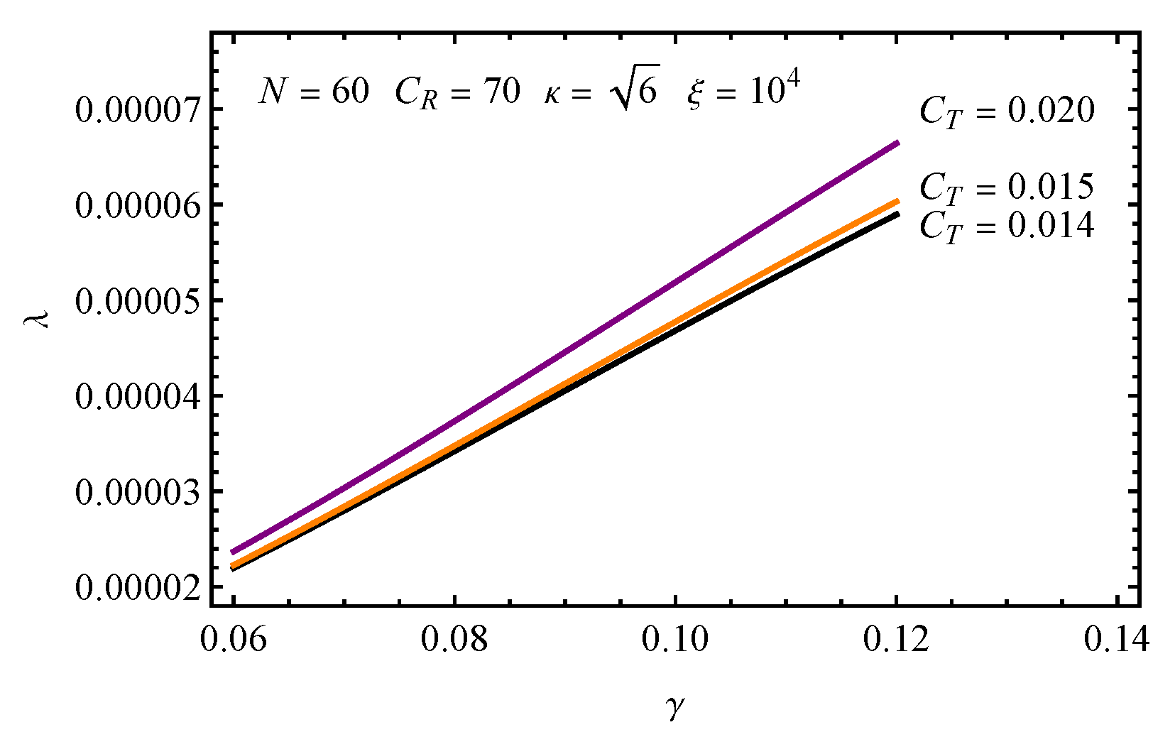
The resulting constraint is plotted in Fig.1 by using the definition of in Eq.(39). The magnitude of needed to produce the observed amplitude of scalar perturbations increases linearly for increasing . For reference, we consider various values of and figure out a pair of in which their values produce the observed amplitude of scalar perturbations. More interestingly, the numerical values of the self-interacting coupling, , shown in Fig.1 are consistent with the results of the running coupling up to two-loop corrections in the standard model of particle physics that is very close to zero at the GUT scale which would be a typical scale of inflation Degrassi et al. 2012. In addition, the values of the coupling is in order and still are much bigger than the unnaturally small of for the minimal coupling cold inflation Guth and Pi 1982; Hamada et al. 2014.
We present the COBE constrained results for relations between the and parameters with varying values of the in Table 1 and then compare the predictions in the plane of the latest Planck 2018 data by using the expressions of the and in Eqs.(42) and (43), respectively with the growing mode in (41).
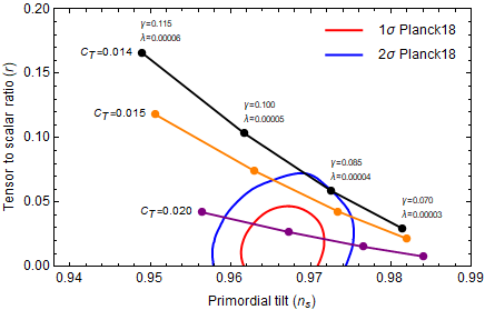

From Fig.2, we present the confidence contours in the plane. The value of is varied for each trajectory. The curves in this figure are related to as: (black), (orange) and (purple) from the bottom curve to the top one. With a set of input parameters when decreases the curve is shifted upward. The proper set of the parameters , , and is used. With these values of the parameters, we find that in order to fit inside the confidence level of the Planck 2018 data, the range of is in and it dose not exceed the upper bound from the constraint of the power spectrum Bastero-Gil et al. 2018b. More importantly, the given range of the parameter , can consequently provide the possible values of the couplings and that are encoded in the as shown in Eq.(29). The allowed region in the parameter space of the and is depicted in Fig.3. To make consistent results between theory and observation, in addition, this requires that the cut-off, of the inflaton field should be less than the Planck mass around one order of magnitude in contrast to cold inflation that usually imposes .
IV Conclusion
In this work, we presented the theoretical study of the non-minimal coupling warm inflation with the quantum-corrected self-interacting inflaton potential. The slow-roll dynamics of warm inflation in the Einstein frame is analyzed by using the dissipative coefficient as linear function of temperature. At the large field approximation in warm inflation, the universal bound for the quantum-corrected parameter, is modified by the dissipative coefficient. With the proper set of the parameters, the universal bound of warm inflation is bigger than that of cold inflation. This indicates that the inflaton field in warm inflation is smaller that of the cold one at the end of inflation. Having used the COBE normalization of the observed amplitude, we found that the relationship between the self-interacting coupling, and the quantum-corrected parameter, is linear and the value of the is in order for . The constraint of the coupling from COBE is consistent with the renormalization group result at the GUT scale. We continuously compared the tensor to scalar ratio () and spectral index () from the theoretical results to the Planck 2018 data. As results, the given sets of the model’s parameters provide good agreement with the Planck 2018 observational data. To make the theoretical results locating inside the 2 confidence level, it was found that the range of the parameter from the dissipative coefficient, is in range and the lower bound of the parameter is constrained in this work. Consequently, we have also used the range of to evaluate the allowed region in the parameter space and in terms of the supersymmetric model that are used to calculate the dissipative coefficient. In addition, the self-interacting coupling, should be very small and this is consistent with the constraint from COBE. More importantly, in contrast to cold inflation scenario, the cut-off scale of the inflaton, is smaller than that of the Planck scale of one order of magnitude to obtain the results compatible with the data. Furthermore, higher order quantum-correction and other form of the inflaton potential are worth for extensively study. More information and accurate observational data might provide more details about the quantum-correction of the inflaton and validity of the warm inflationary universe, especially the observation data of the primordial tensor modes.
Acknowledgements.
D. Samart is financially supported by the Mid-Career Research Grant 2021 from National Research Council of Thailand under a contract No. N41A640145. P. Ma-adlerd is supported by National Astronomical Research Institute of Thailand (NARIT). P. Channuie acknowledged the Mid-Career Research Grant 2020 from National Research Council of Thailand under a contract No. NFS6400117.References
- Berera (1995) A. Berera, Warm inflation, Phys. Rev. Lett. 75, 3218 (1995), arXiv:astro-ph/9509049 .
- Berera and Fang (1995) A. Berera and L.-Z. Fang, Thermally induced density perturbations in the inflation era, Phys. Rev. Lett. 74, 1912 (1995), arXiv:astro-ph/9501024 .
- Berera (1996) A. Berera, Thermal properties of an inflationary universe, Phys. Rev. D 54, 2519 (1996), arXiv:hep-th/9601134 .
- Hall et al. (2004) L. M. H. Hall, I. G. Moss, and A. Berera, Scalar perturbation spectra from warm inflation, Phys. Rev. D 69, 083525 (2004), arXiv:astro-ph/0305015 .
- Berera (2000) A. Berera, Warm inflation at arbitrary adiabaticity: A Model, an existence proof for inflationary dynamics in quantum field theory, Nucl. Phys. B 585, 666 (2000), arXiv:hep-ph/9904409 .
- Berera (2003) A. Berera, Warm inflation solution to the eta problem, PoS AHEP2003, 069 (2003), arXiv:hep-ph/0401139 .
- Ramos (2001) R. O. Ramos, Fine tuning solution for hybrid inflation in dissipative chaotic dynamics, Phys. Rev. D 64, 123510 (2001), arXiv:astro-ph/0104379 .
- Berera and Gordon (2001) A. Berera and C. Gordon, Inflationary initial conditions consistent with causality, Phys. Rev. D 63, 063505 (2001), arXiv:hep-ph/0010280 .
- Bastero-Gil et al. (2018a) M. Bastero-Gil, A. Berera, R. Brandenberger, I. G. Moss, R. O. Ramos, and J. G. Rosa, The role of fluctuation-dissipation dynamics in setting initial conditions for inflation, JCAP 01, 002, arXiv:1612.04726 [astro-ph.CO] .
- Berera et al. (2009) A. Berera, I. G. Moss, and R. O. Ramos, Warm Inflation and its Microphysical Basis, Rept. Prog. Phys. 72, 026901 (2009), arXiv:0808.1855 [hep-ph] .
- Bastero-Gil and Berera (2009) M. Bastero-Gil and A. Berera, Warm inflation model building, Int. J. Mod. Phys. A 24, 2207 (2009), arXiv:0902.0521 [hep-ph] .
- Rangarajan (2019) R. Rangarajan, Current Status of Warm Inflation, in 18th Lomonosov Conference on Elementary Particle Physics (2019) pp. 339–345, arXiv:1801.02648 [astro-ph.CO] .
- Moss and Xiong (2006) I. G. Moss and C. Xiong, Dissipation coefficients for supersymmetric inflatonary models, (2006), arXiv:hep-ph/0603266 [hep-ph] .
- Berera et al. (1998) A. Berera, M. Gleiser, and R. O. Ramos, Strong dissipative behavior in quantum field theory, Phys. Rev. D 58, 123508 (1998), arXiv:hep-ph/9803394 .
- Berera and Ramos (2001) A. Berera and R. O. Ramos, The Affinity for scalar fields to dissipate, Phys. Rev. D 63, 103509 (2001), arXiv:hep-ph/0101049 .
- Zhang (2009) Y. Zhang, Warm Inflation With A General Form Of The Dissipative Coefficient, JCAP 03, 023, arXiv:0903.0685 [hep-ph] .
- Bastero-Gil et al. (2011) M. Bastero-Gil, A. Berera, and R. O. Ramos, Shear viscous effects on the primordial power spectrum from warm inflation, JCAP 07, 030, arXiv:1106.0701 [astro-ph.CO] .
- Bastero-Gil et al. (2013) M. Bastero-Gil, A. Berera, R. O. Ramos, and J. G. Rosa, General dissipation coefficient in low-temperature warm inflation, JCAP 01, 016, arXiv:1207.0445 [hep-ph] .
- Bastero-Gil et al. (2014) M. Bastero-Gil, A. Berera, R. O. Ramos, and J. a. G. Rosa, Observational implications of mattergenesis during inflation, JCAP 10, 053, arXiv:1404.4976 [astro-ph.CO] .
- Berera and Ramos (2003) A. Berera and R. O. Ramos, Construction of a robust warm inflation mechanism, Phys. Lett. B 567, 294 (2003), arXiv:hep-ph/0210301 .
- Bastero-Gil and Berera (2005a) M. Bastero-Gil and A. Berera, Sneutrino warm inflation in the minimal supersymmetric model, Phys. Rev. D 72, 103526 (2005a), arXiv:hep-ph/0507124 .
- Bastero-Gil and Berera (2005b) M. Bastero-Gil and A. Berera, Determining the regimes of cold and warm inflation in the SUSY hybrid model, Phys. Rev. D 71, 063515 (2005b), arXiv:hep-ph/0411144 .
- Bassett et al. (2006) B. A. Bassett, S. Tsujikawa, and D. Wands, Inflation dynamics and reheating, Rev. Mod. Phys. 78, 537 (2006), arXiv:astro-ph/0507632 .
- Martin et al. (2014) J. Martin, C. Ringeval, and V. Vennin, Encyclopædia Inflationaris, Phys. Dark Univ. 5-6, 75 (2014), arXiv:1303.3787 [astro-ph.CO] .
- Grøn (2018) O. Grøn, Predictions of Spectral Parameters by Several Inflationary Universe Models in Light of the Planck Results, Universe 4, 15 (2018).
- Coleman and Weinberg (1973) S. R. Coleman and E. J. Weinberg, Radiative Corrections as the Origin of Spontaneous Symmetry Breaking, Phys. Rev. D 7, 1888 (1973).
- Joergensen et al. (2014) J. Joergensen, F. Sannino, and O. Svendsen, Primordial tensor modes from quantum corrected inflation, Phys. Rev. D 90, 043509 (2014), arXiv:1403.3289 [hep-ph] .
- Panotopoulos and Videla (2015) G. Panotopoulos and N. Videla, Warm inflationary universe model in light of Planck 2015 results, Eur. Phys. J. C 75, 525 (2015), arXiv:1510.06981 [gr-qc] .
- Benetti and Ramos (2017) M. Benetti and R. O. Ramos, Warm inflation dissipative effects: predictions and constraints from the Planck data, Phys. Rev. D 95, 023517 (2017), arXiv:1610.08758 [astro-ph.CO] .
- Motaharfar et al. (2018) M. Motaharfar, E. Massaeli, and H. R. Sepangi, Warm Higgs G-inflation: predictions and constraints from Planck 2015 likelihood, JCAP 10, 002, arXiv:1807.09548 [gr-qc] .
- Kamali (2018) V. Kamali, Non-minimal Higgs inflation in the context of warm scenario in the light of Planck data, Eur. Phys. J. C 78, 975 (2018), arXiv:1811.10905 [gr-qc] .
- Graef and Ramos (2018) L. L. Graef and R. O. Ramos, Probability of Warm Inflation in Loop Quantum Cosmology, Phys. Rev. D 98, 023531 (2018), arXiv:1805.05985 [gr-qc] .
- Arya and Rangarajan (2020) R. Arya and R. Rangarajan, Study of warm inflationary models and their parameter estimation from CMB, Int. J. Mod. Phys. D 29, 2050055 (2020), arXiv:1812.03107 [astro-ph.CO] .
- Bastero-Gil et al. (2018b) M. Bastero-Gil, A. Berera, R. Hernández-Jiménez, and J. a. G. Rosa, Dynamical and observational constraints on the Warm Little Inflaton scenario, Phys. Rev. D 98, 083502 (2018b), arXiv:1805.07186 [astro-ph.CO] .
- Ramos and da Silva (2013) R. O. Ramos and L. A. da Silva, Power spectrum for inflation models with quantum and thermal noises, JCAP 03, 032, arXiv:1302.3544 [astro-ph.CO] .
- Mishra et al. (2012) H. Mishra, S. Mohanty, and A. Nautiyal, Warm natural inflation, Phys. Lett. B 710, 245 (2012), arXiv:1106.3039 [hep-ph] .
- Bastero-Gil et al. (2016) M. Bastero-Gil, A. Berera, R. O. Ramos, and J. G. Rosa, Warm Little Inflaton, Phys. Rev. Lett. 117, 151301 (2016), arXiv:1604.08838 [hep-ph] .
- Graham and Moss (2009) C. Graham and I. G. Moss, Density fluctuations from warm inflation, JCAP 07, 013, arXiv:0905.3500 [astro-ph.CO] .
- Taylor and Berera (2000) A. N. Taylor and A. Berera, Perturbation spectra in the warm inflationary scenario, Phys. Rev. D 62, 083517 (2000), arXiv:astro-ph/0006077 .
- De Oliveira and Joras (2001) H. P. De Oliveira and S. E. Joras, On perturbations in warm inflation, Phys. Rev. D 64, 063513 (2001), arXiv:gr-qc/0103089 .
- Bezrukov et al. (2009) F. Bezrukov, D. Gorbunov, and M. Shaposhnikov, On initial conditions for the Hot Big Bang, JCAP 06, 029, arXiv:0812.3622 [hep-ph] .
- Degrassi et al. (2012) G. Degrassi, S. Di Vita, J. Elias-Miro, J. R. Espinosa, G. F. Giudice, G. Isidori, and A. Strumia, Higgs mass and vacuum stability in the Standard Model at NNLO, JHEP 08, 098, arXiv:1205.6497 [hep-ph] .
- Guth and Pi (1982) A. H. Guth and S. Y. Pi, Fluctuations in the New Inflationary Universe, Phys. Rev. Lett. 49, 1110 (1982).
- Hamada et al. (2014) Y. Hamada, H. Kawai, K.-y. Oda, and S. C. Park, Higgs Inflation is Still Alive after the Results from BICEP2, Phys. Rev. Lett. 112, 241301 (2014), arXiv:1403.5043 [hep-ph] .