Data analysis of effective Hamiltonians in iron-based superconductors
— Construction of predictors for superconducting critical temperature
Abstract
High-temperature superconductivity occurs in strongly correlated materials such as copper oxides and iron-based superconductors. Numerous experimental and theoretical works have been done to identify the key parameters that induce high-temperature superconductivity. However, the key parameters governing the high-temperature superconductivity remain still unclear, which hamper the prediction of superconducting critical temperatures (s) of strongly correlated materials. Here by using data-science techniques, we clarified how the microscopic parameters in the effective Hamiltonians correlate with the experimental s in iron-based superconductors. We showed that a combination of microscopic parameters can characterize the compound-dependence of using the principal component analysis. We also constructed a linear regression model that reproduces the experimental from the microscopic parameters. Based on the regression model, we showed a way for increasing by changing the lattice parameters. The developed methodology opens a new field of materials informatics for strongly correlated electron systems.
I Introduction
The discovery of the high- superconductivity in the copper oxides has inspired a huge amount of studies to clarify the relation between electronic correlations and high- superconductivityKeimer2015. In 2008, the discovery of another high- superconductivity in iron-based superconductors renewed the interest in the superconductivity induced by the electronic correlationsKamihara2008. Theoretical and experimental studies of these high- superconductors have revealed that electronic correlations such as Coulomb interactions are key factors that stabilize the high- superconductivity.RevModPhys.83.1589; HOSONO2015399; si2016high However, it remains unclear how the electronic correlations correlate with .
Recent theoretical progress enables us to determine the microscopic parameters in the low-energy effective Hamiltonians of solids in an way. The method is often referred to as the downfolding methodImada2010. Through this method, based on the band structures obtained from the density functional theory (DFT) calculations, screened interactions (e.g., Coulomb interactions) in the low-energy effective Hamiltonians are calculated using the constrained random phase approximation (cRPA) methodAryasetiawan2004. By solving the low-energy effective Hamiltonians, we can evaluate the physical properties of strongly correlated materials in a fully way beyond the DFT calculations. It has been shown that the scheme can reproduce the ground-state phase diagrams of the high- superconductorsMisawa2014; Ohgoe2020.
The combination of an downfolding scheme and an accurate analysis of the derived Hamiltonians is useful for clarifying the mechanism of the high- superconductivity. However, application of this method has been limited to a few compounds due to the high numerical cost associated with the accurate analysis of the effective Hamiltonians. The difficulty of solving the effective Hamiltonians prevents us from gaining a deep understanding of the high- superconductivity and designing new high- superconductors. Therefore, to predict new superconductors based on the theoretical calculations, development of an alternative and efficient method without solving Hamiltonians is desirable.
Data-driven approaches, such as high-throughput screening, regression analysis, and multivariate statistics, have been used for discovering and designing new compounds with high functionalityHimanen2019. Stimulated by the recent progress of data-science, data-driven analyses focused on superconductors have been performedKlintenberg2013possible; Isayev2015materials; Owolabi2015estimation; Stanev2018machine; Matsumoto2019acceleration; Konno2021deep; Roter2020; Liu2020; Akomolafe2021. For example, in Ref. Stanev2018machine, utilizing the existing database, the authors constructed regression models for predicting based on the information of the chemical-composition data of the compounds and the DFT calculations. Their analysis offers several important insights into the relation between the chemical composition and . However, the effects of electronic correlations in the compounds have not been directly considered in the existing database. Electronic correlations are key factors that stabilize the high- superconductivity and hence the analysis of datasets that explicitly include the information about the electronic correlations is desirable.
From the early stage of studies of the iron-based superconductors, it has been demonstrated that the approach such as the derivation of the band structures and the effective Hamiltonians is useful for clarifying the magnetism Singh_PRL2008; ZPYin_PRL2008 and superconductivity Kuroki_RPL2008; Mazin_PRL2008; Kuroki_PRB2009. In particular, evaluations of the microscopic parameters in the effective Hamiltonians give an insight in understanding the variety of the iron-based superconductors miyake2010comparison. In this paper, to elucidate the relation between the compound dependence of and the microscopic parameters, we derive the low-energy effective Hamiltonians for 32 iron-based superconductors and 4 related compounds. These superconductors offer an ideal platform for examining the relation between and the correlation effects because and the strength of the correlations largely depend on the compounds.
Based on the obtained low-energy effective Hamiltonians, rather than directly solving the Hamiltonians, we analyze the relations between the experimentally observed and the microscopic parameters comprising these Hamiltonians. This analysis is performed using the data-science techniques such as principal component analysis (PCA) and construction of a linear regression model. Through the PCA, we find that the compound dependence is well characterized by the first and second principal components and that the first (second) component consists mainly of the Coulomb interactions (hopping parameters). For example, we find that 1111 compounds have a similar first component and the difference in these compounds is characterized by the second component. We also show that the compound dependence of with respect to the second principal component is manifested as a dome structure. This result indicates that the microscopic parameters comprising the effective Hamiltonians provide sufficient information for describing the compound dependence.
We also construct a linear regression model, which reproduces the experimentally observed from the microscopic parameters comprising the effective Hamiltonians. The obtained model succeeds in reproducing the materials dependence of , as evidenced by a high coefficient of determination (). We show that our regression model can predict a way to enhance the of LaFeAsO by changing the structure of the material.
This paper is organized as follows: In Sec. II, we denote the basics of the target materials and explain the downfolding method. In Sec. III.1, we show the compound dependence of the microscopic parameters including the electronic correlations in the obtained low-energy effective Hamiltonians. In Sec. III.2, we perform PCA aimed at identifying the main parameters that describe the iron-based superconductors using the obtained Hamiltonians. We also construct a regression model that reproduces from the microscopic parameters. Based on this model, we show a way to optimize of the iron-based superconductors. A summary and issues that will be addressed in future work are presented in Sec. IV.
II Method
In this section, we briefly explain the numerical methods we employed, namely the downfolding method, the PCA, and the construction of a linear regression model.
II.1 downfolding method
The DFT calculations of the target materials are performed using QUANTUM ESPRESSOGiannozzi2017. As the pseudopotential set, we use sg15 librarySchlipf2015, which includes the optimized norm-conserving Vanderbilt pseudopotentials (ONCVPSP)Hamann2013. We replace the pseudopotentials for Gd, Nd, Pr, Ce, and Sm, and Tb with that of La to eliminate the metallic bands around the Fermi energy. This approach has been already applied to derivation of parameters for cuprates with a lanthanoidJang_srep2016. We use a -mesh in the first Brillouin zone to perform self-consistent calculations. The optimized tetrahedron method is employed for the DFT calculationsKawamura2014. An energy cutoff of 120 (480) Ry is set for plane waves (charge densities).
To derive effective Hamiltonians for our target materials, we use RESPACK Nakamura2021. In this work, we construct effective models that are the ten-orbital models consisting of 3 orbitals associated with transition metals (TMs), e.g., Fe, Mn, and Ni. The Hamiltonians are given as follows.
| (1) | ||||
| (2) | ||||
| (3) |
where ( ) denotes the creation (annihilation) operator of an electron with spin at the -th maximally localized Wannier function (MLWF)Marzari1997; Souza2001. The indices of the MLWFs include the position of the unit cell , the orbital degrees of freedom and the index of the TM , i.e., . Note that the unit cell contains two TMs. in the one-body part of the effective Hamiltonians () represents the hopping parameters of an electron with spin between the -th and -th MLWFs. When we construct the MLWFs, the - axis is rotated by from the - axis of the unit cell. For this condition, the - axis is parallel to the nearest TM-TM directions. Two-body interactions such as Coulomb interactions () and the exchange interactions () are obtained via cRPA calculationsAryasetiawan2004. We set an energy cutoff of 20 Ry for the dielectric function and calculate dielectric functions using more than 100 bands. In both calculations, we use points for the 122 systems and points for the others.
The downfolding method based on cRPA has been applied to a wide range of the correlated electron systems including iron-based superconductors miyake2010comparison; Aichhorn_PRB2010 and cuprates Jang_srep2016; Hirayama_PRB2019; Nilsson_PRB2019. Through these applications, it is shown that the downfolding method gives realistic values of the Coulomb and exchange interactions. However, there are several variations of the cRPA method such as the treatment of the band disentangle Souza2001; Miyake_PRB2009; Sasioglu2011. The quantitative results may depend on the details of the methods. For example, in the derivation of the single-band Hubbard-type Hamiltonians of the cuprates, it is pointed out Nilsson_PRB2019 that the values of onsite Coulomb interactions depend on the downfolding methods Jang_srep2016; Hirayama_PRB2019; Nilsson_PRB2019. We expect that this subtle problem does not exist in the derivation of the ten-orbital Hamiltonians in the iron-based superconductors since the ten bands cover almost all the degrees of freedom near the Fermi energy. Therefore, we use the cRPA method with the conventional band-disentanglement treatment Souza2001 implemented in RESPACK to capture the overall trend of the compound dependence of the effective Hamiltonians.
For the 122 family, an model including orbitals of alkaline earth metals such as Ba is more appropriate (than other models) because these bands are located above but near the Fermi levelUsui2019. Nevertheless, using 10 orbitals in TM atoms, we can construct the MLWFs that reproduce the DFT band structure below the energy associated with the band of alkaline earth metals.
Using the derived microscopic parameters, we employ the following typical parameters as descriptors for the data analysis,
| (4) | ||||
| (5) | ||||
| (6) | ||||
| (7) | ||||
| (8) | ||||
| (9) |
where is a primitive translation vector along the axis. specifies orbital information; , and . is a function for extracting a feature of the derived microscopic parameters among all combinations of and . We use three types of : a function that returns the maximum value (p=max), a function that returns the mean value (p=mean), and a function that returns the minimum value (p=min). We exclude and because these are zero. Throughout this paper, , , , and for simplicity.
II.2 PCA
It is expected that the difference in the parameters of the derived effective Hamiltonians can characterize various target materials. To verify this hypothesis, we visualize the relationship between the parameters and extract the main parameters that govern the materials dependence via PCA. The PCA, which has been applied to a dataset obtained for superconductors Rajan2009, leads to a reduction in the dimensionality of a dataset, thereby providing information on the principal components of the target dataset. We note that the results of PCA depend on the employed data set. In this study, we perform PCA analysis for the Hamiltonians of the compounds with high to clarify the microscopic parameter dependence of .
Here, we briefly explain basics of the PCA Bishop2006. Using the descriptor vector of the -th data (where corresponds to the index of materials), we construct the covariance matrix , which is defined as
| (10) |
where is the total number of the materials. We note that the average value of the descriptors over the materials is set to 0 () and its standard deviation is set to 1. By diagonalizing , we obtain the principal vectors with the principal values (’s are sorted in descending order). The first principal vector represents the direction associated with the most diverse data. Using the principal vectors , we can project the descriptor vectors onto the principal vectors and obtain the th principal value as follows,
| (11) |
In Sec. III.2, we show that the materials dependence can be characterized by the principal values.
II.3 Construction of regression model
We construct a linear regression model for reproducing from the parameters of the effective Hamiltonian,
| (12) |
To introduce non-linearity, we inserted the quadratic terms and the ratio terms (such as and ) between the original parameters. (please see Appendix A for further details of the descriptors).
The number of samples in our dataset is comparable to that of the descriptors, and hence we should carefully control the number of the descriptors in the regression models to avoid overfitting. Therefore, we prepared models where some descriptors were dropped in a systematic way — for example, one model has only hopping parameters as descriptors, another one has hopping and onsite-Coulomb interactions, and yet another one has hopping, onsite-Coulomb and the cross term between these parameters (for details, see Appendix A). To identify the optimal model among these models, we calculate the scores associated with each model. One of the simplest ways to estimate score is the hold-out validation (HV) method [Fig. 1 (a)]. For this method, we first split the original dataset (white boxes in Fig. 1) into two parts, the training dataset (blue boxes) and the validation dataset (red boxes). The model is optimized by using the training dataset and a training algorithm with the hyperparameter . The score of the model is calculated as follows,
| (13) |
where is the validation dataset, is the experimental of the material labeled with and is the number of the validation data. The model with a minimum score is chosen as the optimal model.
While the HV method has a bias from how to split the dataset, the cross-validation (CV) method reduces it. In this study, we employ the nested CV method stone1974cross, whose procedure is shown in Fig. 1 (b). In the following, we explain the procedure of the nested CV method.
(i) Outer CV: We first split the original dataset by the leave-one-out CV (LOOCV) method, which corresponds to the outer CV. In the outer CV, each model is trained by an algorithm with its hyperparameter .
(ii) Inner CV: To tune for -th split dataset as , we again apply the LOOCV method to the training data with samples of -th training dataset, which is called the inner CV.
(iii) Determination of : In this inner CV process, we optimize the weights of the model by minimizing LASSO (least absolute shrinkage and selection operator)tibshirani1996regression type cost function;
| (14) |
where is the -th training dataset in the inner CV and is the number of data in , and the coefficient of the term, is a hyper parameter of LASSO, which will be tuned by the inner CV. By using obtained , the score for the model and -th dataset split from -th dataset in the outer CV, is calculated as
| (15) |
After scores for all inner CV dataset are obtained, the total score of
| (16) |
is calculated. Finally, the hyperparameter is tuned to minimize . Note that the -th dataset split by the outer CV is split further into samples for training () and one sample for validation () in the inner CV. We use scikit-learn scikit-learn package to solve the LASSO and use Optuna optuna_2019 to optimize by means of the Bayesian optimization method.
(iv) Evaluation of score: After is optimized, the weight of the model , in following equation is again optimized by LASSO with as in the normal CV method, and then the validation score defined in Eq. (17) is evaluated as follows:
| (17) |
where is the -th validation dataset split by the outer CV and .
(v) Average of score: The final score is then calculated from the following equation.
| (18) |
(vi) Determination of the best model: By performing the nested CV for all the models we define, we obtain the best model with the lowest score, i.e. .

III Results
III.1 results
We obtain the low-energy effective Hamiltonians for the 11-family (e.g., FeSe), 1111-family (e.g., LaFeAsO), 111-family (e.g., LiFeAs), 122-family (e.g., BaFe2As2), and 42622-family (e.g., Ca4Al2O6Fe2As2). For comparison with the iron-based superconductors, we have also obtained the low-energy effective Hamiltonians for Mn (e.g., BaMnAsF) and Ni (e.g., LaNiAsO) analogs of the iron-based superconductors. Each target material is categorized as one of the above-mentioned families based on the chemical composition of the materials.
The typical microscopic parameters (such as the maximum values of the hopping parameters and the averaged onsite-Coulomb interactions) comprising the low-energy effective Hamiltonians and the families of our target compounds are listed in Table 1. The numerical conditions of the calculations are detailed in Sec. II.1. The crystal structures of all the target materials except for , GdFePO and NdFePO are obtained from the experiments. Most of them are obtained from the Inorganic Crystal Structure Database (ICSD)bergerhoff1983inorganic; zagorac2019recent and SpringerMaterialsspringer_materials. We note that we employ a tetragonal crystal phase at ambient pressure. For calculations of (GdFePO and NdFePO), the fractional coordinates of the atoms are used as the same as those of (PrFePO), and the lattice constant is employed from the experiment.
We find that the amplitudes of the hopping parameters and the Coulomb interactions exhibit a strong dependence on the compounds. For example, of FeSe ( = 10.11) is approximately twice that of GdFePO ( = 5.15). This significant variation indicates that iron-based superconductors offer an ideal platform for examining the relation between and the microscopic parameters. We note that the overall tendency of the obtained parameters is consistent with the tendency revealed by previous calculations miyake2010comparison; miyake2010_42622. In particular, the averaged Coulomb interaction values agree (to within 10%) with those obtained in the previous studies, except for BaFe2As2. The value of BaFe2As2 is 20% smaller than that reported in the previous study miyake2010comparison. This deviation may have resulted from the difference between the disentangle treatment for the Ba band near the Fermi level. We neglect clarification of this difference because (in the present study) we focus on the relation between the and overall compound dependence of the microscopic parameters.
| material | family | (eV) | (eV) | (eV) | (eV) | Ref | |||
| FeS | 11 | 0.46 | 4.53 | 1.20 | 0.55 | 9.91 | 2.63 | 1.21 | str_FeS |
| FeSe | 11 | 0.41 | 4.14 | 1.04 | 0.55 | 10.11 | 2.53 | 1.33 | str_FeSe |
| FeTe | 11 | 0.37 | 3.15 | 0.73 | 0.50 | 8.57 | 1.98 | 1.37 | str_FeTe |
| CaFeAsH | 1111 | 0.37 | 2.71 | 0.70 | 0.44 | 7.26 | 1.88 | 1.19 | str_CaFeAsH |
| SrFeAsF | 1111 | 0.37 | 3.13 | 0.88 | 0.47 | 8.44 | 2.38 | 1.26 | str_SrFeAsF |
| CaFeAsF | 1111 | 0.38 | 3.01 | 0.87 | 0.46 | 7.96 | 2.30 | 1.21 | str_CaFeAsF |
| LaFePO | 1111 | 0.43 | 2.40 | 0.65 | 0.40 | 5.59 | 1.51 | 0.92 | str_LaFePO |
| PrFePO | 1111 | 0.43 | 2.44 | 0.65 | 0.40 | 5.62 | 1.51 | 0.93 | str_GdFePO_SmFePO_PrFePO_NdFePO |
| NdFePO | 1111 | 0.44 | 2.44 | 0.66 | 0.40 | 5.51 | 1.49 | 0.90 | str_GdFePO_SmFePO_PrFePO_NdFePO |
| SmFePO | 1111 | 0.45 | 2.44 | 0.66 | 0.40 | 5.45 | 1.47 | 0.89 | str_GdFePO_SmFePO_PrFePO_NdFePO |
| GdFePO | 1111 | 0.47 | 2.40 | 0.66 | 0.39 | 5.15 | 1.41 | 0.84 | str_GdFePO_SmFePO_PrFePO_NdFePO |
| LaFeAsO | 1111 | 0.36 | 2.46 | 0.61 | 0.43 | 6.90 | 1.72 | 1.19 | Kamihara2008 |
| CeFeAsO | 1111 | 0.36 | 2.49 | 0.62 | 0.43 | 6.88 | 1.72 | 1.18 | str_CeFeAsO |
| PrFeAsO | 1111 | 0.36 | 2.50 | 0.62 | 0.43 | 6.91 | 1.72 | 1.19 | str_NdFeAsO_PrFeAsO_SmFeAsO_TbFeAsO |
| NdFeAsO | 1111 | 0.36 | 2.51 | 0.62 | 0.44 | 6.95 | 1.71 | 1.22 | str_NdFeAsO_PrFeAsO_SmFeAsO_TbFeAsO |
| SmFeAsO | 1111 | 0.37 | 2.51 | 0.63 | 0.43 | 6.84 | 1.71 | 1.17 | str_NdFeAsO_PrFeAsO_SmFeAsO_TbFeAsO |
| GdFeAsO | 1111 | 0.37 | 2.52 | 0.63 | 0.44 | 6.73 | 1.67 | 1.16 | str_GdFeAsO |
| TbFeAsO | 1111 | 0.37 | 2.52 | 0.63 | 0.43 | 6.76 | 1.69 | 1.15 | str_NdFeAsO_PrFeAsO_SmFeAsO_TbFeAsO |
| LiFeP | 111 | 0.50 | 3.09 | 0.90 | 0.45 | 6.23 | 1.82 | 0.90 | str_LiFeP |
| LiFeAs | 111 | 0.42 | 3.02 | 0.78 | 0.47 | 7.17 | 1.86 | 1.12 | str_LiFeAs |
| NaFeAs | 111 | 0.39 | 3.06 | 0.79 | 0.48 | 7.86 | 2.02 | 1.23 | str_NaFeAs |
| 122 | 0.34 | 2.43 | 0.61 | 0.45 | 7.20 | 1.81 | 1.32 | str_KFe2P2; Villars2016:sm_isp_sd_2110357 | |
| 122 | 0.46 | 2.72 | 0.74 | 0.43 | 5.86 | 1.59 | 0.93 | str_SrFe2P2 | |
| 122 | 0.42 | 2.81 | 0.60 | 0.52 | 6.75 | 1.44 | 1.24 | str_SrFe2As2 | |
| 122 | 0.45 | 2.51 | 0.64 | 0.43 | 5.56 | 1.42 | 0.95 | str_BaFe2P2 | |
| 122 | 0.47 | 3.07 | 0.94 | 0.46 | 6.59 | 2.03 | 0.98 | str_KFe2As2 | |
| 122 | 0.37 | 2.62 | 0.64 | 0.44 | 7.09 | 1.74 | 1.20 | str_SrFe2As2 | |
| 122 | 0.37 | 2.38 | 0.52 | 0.44 | 6.36 | 1.39 | 1.18 | str_CaFe2As2 | |
| 122 | 0.36 | 2.40 | 0.55 | 0.45 | 6.59 | 1.50 | 1.22 | str_BaFe2As2 | |
| 42622 | 0.41 | 2.99 | 0.86 | 0.45 | 7.31 | 2.11 | 1.09 | str_Sr4Sc2O6Fe2P2 | |
| 42622 | 0.42 | 3.00 | 0.93 | 0.45 | 7.10 | 2.21 | 1.07 | str_Ca4Al2O6Fe2P2_Ca4Al2O6Fe2As2 | |
| 42622 | 0.41 | 2.95 | 0.90 | 0.45 | 7.12 | 2.16 | 1.09 | str_Ca4Al2O6Fe2P2_Ca4Al2O6Fe2As2 | |
| BaMnAsF | Mn | 0.29 | 2.75 | 0.77 | 0.45 | 9.43 | 2.64 | 1.55 | str_BaMnAsF |
| Mn | 0.31 | 2.33 | 0.57 | 0.43 | 7.47 | 1.82 | 1.36 | str_BaMn2As2 | |
| Ni | 0.42 | 2.81 | 0.48 | 0.47 | 6.64 | 1.15 | 1.11 | str_BaNi2As2 | |
| LaNiAsO | Ni | 0.39 | 2.81 | 0.61 | 0.44 | 7.11 | 1.55 | 1.11 | str_LaNiAsO |
In Fig. 2 (a-d), we plot the compound dependence of the typical microscopic parameters. We find that the effective onsite interaction value of the target materials varies significantly (from five to ten). A significant variation was also noted in Ref. miyake2010comparison where six iron based superconductors were analyzed. The Hund coupling is also dependent on the materials, although its range is narrower than that of .
From the results obtained for the 1111 family, the compounds can be classified into three categories, namely 1111 compounds with P (1111-P), with As (1111-As), and with F or H (1111-F,H). We find that stronger effective Coulomb interactions occur in 1111-F,H than in the other 1111 compounds, owing to the larger compared with those of 1111-P and 1111-As. However, the difference between the values of 1111-P and 1111-As stems from transfer integrals associated with the difference in the localization of MLWF, as noted in Ref. miyake2010comparison. A similar tendency is observed for the 111 family.
The parameters of the relevant compounds are similar to those of iron-based superconductors. Mn compounds have strong effective interactions , which arise from the smaller hopping integrals than those of other compounds. We note that their occupation numbers in one TM atom are different from those of iron-based superconductors.

Before performing the data-science analyses such as PCA, we examine the influence of the lattice structure on the materials dependence of the microscopic parameters. The importance of the anion [chalcogen (Ch) or pnictide (Pn)] position is pointed out in the previous studies Lee2008effect; Mizuguchi2010review, and hence we plot the typical microscopic parameters as a function of the distance between Ch/Pn and TM [see Fig. 2(e-h)]. As shown in Fig. 2 (e), the magnitude of the effective onsite Coulomb interaction increases with increasing distance. As shown in Fig. 2 (f) and (g), we find that this trend is mainly governed by , i.e., decreases almost monotonically with increasing the distance whereas is almost independent of the distance. This result indicates that the difference between the distances controls mainly through the hybridization between TM orbitals and Ch/Pn orbitals. We note that exhibits no clear distance dependence.
III.2 Data analysis
By using the effective Hamiltonians reported in the previous section, we perform the PCA and the regression analysis for of iron-based superconductors. We focus on the superconductivity of the iron-based superconductors in this study, since the values of Ni compounds are very low, and Mn compounds exhibit no superconductivity. The results obtained from our data analysis are summarized in Table 2. We provide details of the PCA analysis and the construction of the regression model in subsequent sections.
Here, we detail our strategy for assigning to the effective Hamiltonians. Since the superconductivity appears in the doped compounds, it is the best way to derive the low-energy effective Hamiltonians for the doped compounds. When we can obtain the information of the lattice structures for both end compounds (e.g. FeSe and FeTe), we interpolate the microscopic parameters of the effective Hamiltonians for the end compounds as shown in Table 2. However, information of the lattice structures for the end compounds is not available in most cases for 1111 compounds. Nevertheless, in terms of the microscopic parameters, we can expect the difference is small in the low-doping regime where shown in Table 2 was observed. Therefore, we simply assume that the effective Hamiltonian of the closest stoichiometry compound can govern the superconductivity in the doped compounds. As we will show, the PCA analysis shows that the combination of the microscopic parameters well describe the compounds dependence of . This result supports the validity of the assumption. We also note that the same assumption was used in the analysis of the relation between and the onsite Coulomb interactions in cuprates Jang_srep2016; Nilsson_PRB2019.
| material | family | (K) | (K) | Hamiltonian | ||
| 11 | 5 str_FeS | 6.2 | -14.89 | 2.07 | ||
| 11 | 13.5 Tc_FeSe_Mizuguchi2008 | 13.4 | -10.51 | -2.79 | ||
| 11 | 23.5note1; Tc_FeSeTe_Noji2012 | 24.3 | -4.56 | -4.63 | (,) | |
| 1111 | 47.4 Tc_CaFeAsH_Muraba2014 | 55.1 | 0.98 | -1.33 | ||
| 1111 | 56 Tc_SrFeAsF_Wu2009 | 51.1 | -3.33 | -2.68 | ||
| 1111 | 56 Tc_CaFeAsF_Cheng2009 | 53.6 | -3.33 | -1.43 | ||
| 1111 | 6.6 Tc_LaNdPrFePO_Baumbach2009 | 3.2 | 3.97 | 2.86 | ||
| 1111 | 3.2 Tc_LaNdPrFePO_Baumbach2009 | 8.2 | 3.54 | 3.49 | ||
| 1111 | 3.1 Tc_LaNdPrFePO_Baumbach2009 | 4.6 | 3.46 | 3.65 | ||
| 1111 | 3 Tc_SmFePO_Kamihara2008 | 6.4 | 3.39 | 4.13 | ||
| 1111 | 6.1 Tc_GdFePO_Liang2010 | 2.5 | 3.33 | 5.90 | ||
| 1111 | 29 note2; Tc_LaFeAsO_Iimura2012 | 43.3 | 4.60 | -3.27 | ||
| 1111 | 47 Tc_CeFeAsO_Matsuishi2012 | 46.1 | 4.15 | -2.59 | ||
| 1111 | 52 Tc_PrFeAsO_Ren2008 | 48.4 | 4.05 | -2.41 | ||
| 1111 | 52.8 Tc_NdFeAsO_Adamski2017 | 55.2 | 3.85 | -2.00 | ||
| 1111 | 55.6 Tc_SmFeAsO_Kamihara2010 | 48.1 | 3.61 | -1.92 | ||
| 1111 | 53.5 Tc_GdFeAsO_Yang2008 | 49.5 | 3.26 | -0.95 | ||
| 1111 | 50 Tc_TbFeAsO_Yates2009 | 46.9 | 3.23 | -1.49 | ||
| 111 | 6 str_LiFeP | 5.7 | -5.44 | 6.67 | ||
| 111 | 26 Tc_NaFeAs_Wang2009 | 24.1 | -1.89 | -3.14 | ||
| 111 | 18 Tc_LiFeAs_Wang2008 | 28.1 | -2.60 | 0.55 | ||
| 122 | 27 Tc_SrFe2AsP2_Shi2010 | 31.0 | 2.15 | 0.77 | (,) | |
| 122 | 31 Tc_BaFe2AsP2_Kasahara2010 | 33.0 | 4.73 | -0.64 | (,) | |
| 122 | 37 Tc_KSrFe2As2_Sasmal2008 | 26.1 | -1.17 | 0.65 | (,) | |
| 122 | 48 note3; Tc_CaFe2As2_Kudo2013 | 49.0 | 6.17 | -0.79 | ||
| 122 | 38.7 Tc_BaKFe2As2_Rotter2008 | 29.2 | 1.03 | -0.20 | (,) | |
| 42622 | 17.1 str_Ca4Al2O6Fe2P2_Ca4Al2O6Fe2As2 | 19.2 | -5.29 | 0.66 | ||
| 42622 | 17 str_Sr4Sc2O6Fe2P2 | 18.8 | -2.11 | 0.98 | ||
| 42622 | 28.3 str_Ca4Al2O6Fe2P2_Ca4Al2O6Fe2As2 | 26.9 | -4.37 | -0.13 |

III.2.1 PCA
Before showing the results of PCA, we first examine how depends on the typical microscopic parameters such as , , and . As shown in Fig.3, We do not find any significant correlation between and . On the other hand, we find that shows a subtle peak structure as a function and . This is in sharp contrast with the cuprates where it is proposed that has some correlations with both and Jang_srep2016; Nilsson_PRB2019. As we show later, from the PCA analysis, we show that shows a clear peak structure as a function of the second principal component, which mainly consists of the hopping parameters. Thus, although this dependence roughly captures some aspects of the compound dependence of , the PCA analysis is a more systematic way for extracting the important descriptors for characterizing the target systems without any prior knowledge.
Here, we explain why the parameter dependence of is different between iron-based superconductors and cuprates. In iron-based superconductors, the hopping parameters, such as , mainly change while the Coulomb interactions, such as , mainly change in cuprates Jang_srep2016; Nilsson_PRB2019; Jean2022; Hirayama2022. This difference can be understood as follows: In iron-based superconductors, the distance between anions and irons (e.g., As and Fe) widely varies, as shown in Fig. 2. This indicates that the hybridizations between anions and irons, i.e., the amplitudes of the hopping parameters also widely vary. In contrast, in cuprates, the distance between Cu and O in the CuO2 plane does not largely depend on compounds. Thus, the amplitude of the hopping parameters does not largely change in cuprates. This difference in the lattice structures induces the different parameter dependence of . Nevertheless, we note that the normalized electron correlation plays some role in stabilizing high- superconductivity since changes in both iron-based superconductors and cuprates.
For performing the PCA, we employ microscopic parameters as the descriptors, which consist of the Coulomb interactions (), the Hund couplings (), and the hopping parameters (). We obtain , and as the five dominant principal values. The first and the second principal values are large compared with the other principal values, and hence it is expected that the first and the second principal vectors ( and ) accurately reflect the material dependence. In Fig. 4(a), we plot the absolute value of each component comprising these vectors. We find that the interaction parameters (such as onsite and offsite Coulomb interactions) govern the first principal vector while the hopping parameters and Hund couplings govern the second principal vector.
We plot the first and the second principal components ( and ) in Fig. 4(b). For 1111 and 111 compounds, we find that the second component characterizes the differences within families, i.e., the same family has a similar first component, but each compound in the family has a different second component. For example, the first component of the 1111 family is approximately four, but the second component varies from -3.2 to 6.0. In contrast, we find that 122 and 42622 compounds exhibit opposite tendencies: the same family has a similar second component, but each compound has a different first component. We note that the first component changes significantly by changing the total electron density for 1111 and 122 families.
The 11 family exhibits exceptional behavior, i.e., both the first and the second components exhibit considerable compound dependence. This exceptional behavior may be related to exotic phenomena such as the absence of antiferromagnetic order and the high- superconductivity in a monolayer occurring in FeSehsu2008superconductivity; li2009first; Qing2012.
In Fig. 4(c) and (d), we plot as a function of the first and the second principal components. We find that is better correlated with the second component than the first component. In particular, we find that the dependence of on the second component is manifested as a dome structure reminiscent of Lee’s plot Lee2008effect; Mizuguchi2010review. This result indicates that the difference in the microscopic parameters associated with the effective Hamiltonians provides sufficient information for explaining the compound dependence of . By constructing the regression model for reproducing , we show that these parameters allow quantitative reproduction of this dependence.
III.2.2 Regression model for estimating
After determining the best regression model within the nested CV approach explained in Sec. II, we obtain our predictor using all the data obtained in the experiments. Figure 5(a) shows the accuracy of the obtained regression model. We find that this model reproduces the experimental data, as indicated by the high coefficient of determination (). This result confirms that our regression model can predict the of associated with several different families for iron-based superconductors.
We apply our predictor to low-energy Hamiltonians for a hypothetical compound, whose lattice structure is systematically changed from that of LaFeAsO. We vary the fractional coordinates of two As atoms as (0.5, 0.0, ) and (0.0, 0.5, 1-); is the fractional coordinate of As for the original LaFeAsO, namely Kamihara2008, and the parameter indicates changes in the height of As from the Fe plane. A schematic showing this lattice distortion is presented in the inset of Fig. 5(b). Note that the fractional coordinates of the other atoms and the lattice constants do not change.
We obtain the low-energy effective Hamiltonians for the hypothetical compounds. From the microscopic parameters in the Hamiltonians, we calculate the of each compound using the regression model. In Fig. 5(b), we show the dependence of for hypothetical LaFeAsO materials. We find that increases with increasing and vice versa. At , reaches 100K. The applicability range of the regression model is limited to the parameter space around the existing compounds, and therefore the role of lattice distortion in inducing high- superconductivity (K) remains unclear. Nevertheless, the qualitative behavior of may be correctly predicted by the regression model. This result indicates that our regression model captures the essence of Lee’s plotLee2008effect; Mizuguchi2010review and the theoretical study Kuroki_PRB2009, which suggests that the height of As from the Fe plane plays a key role in determining the compound dependence of .
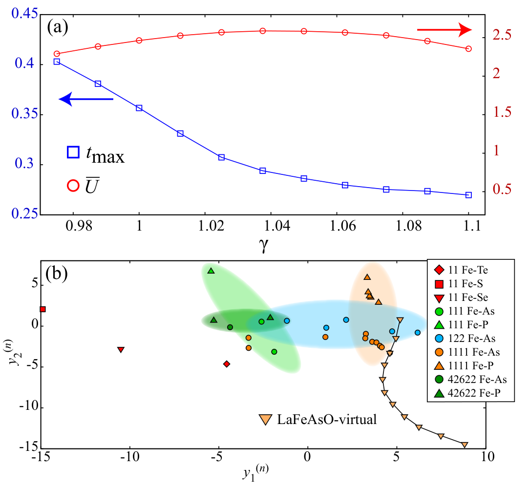
Here, we examine the relation between enhancement of and the microscopic parameters. As shown in Fig. 6(a), the maximum value of the nearest hoppings decreases by increasing while has a broad peak around . This result indicates that we can enhance of LaFeAsO by increasing the amplitude of the electronic correlations. In Fig. 6(b), we plot the first and the second principal components for the virtual materials. We find that the changes in the second principal component governs the enhancement of around LaFeAsO. This plot also indicates that LaFeAsO is located at the edge of the existing materials in the plane. Therefore, it is plausible that we can reach the unexplored region and enhance by changing the height of As in LaFeAsO.
We also consider the possibility of realizing hypothetical materials. In our ab initio calculations of such materials, we do not perform the structure optimization and simulations for phonon’s properties. Therefore, our proposed materials may be unattainable for the conventional bulk system at ambient pressure. Stable materials may be used to obtain an interface structure. Such interface or thin-film structures induce drastic changes in the electronic states of target materials and may enhance . Successful experiments applying this approach have already been reported for high- superconductors such as and FeSe Wu2013; Qing2012. The material structure can also be controlled via laser irradiation, which has been successfully applied to FeSeSuzuki2019. In that work, strong laser irradiation led to changes in the height of Se atoms from the Fe-Fe plane. This results from the displacive excitation of coherent phonon mechanismZeiger1992, which governs the excitation of Raman active modes. These modes also occur in LaFeAsOHadjiev2008, and hence we expect that our predicted structure would be realized via laser irradiation.

IV Summary
In summary, we have derived the low-energy effective Hamiltonians for 32 iron-based compounds and four related compounds using the downfolding method. We have found that microscopic parameters such as the hopping parameters and the Coulomb interaction are associated with a wide range of iron-based superconductors. To systematically characterize the compound dependence of the microscopic parameters, we perform the PCA. As a result, we find that the first principal vector consists of mainly interaction terms, while the second consists of mainly hopping terms. We show that the first principal values characterize the difference within the 42622 and 122 families while the second principal values characterize the difference within the 1111 and 111 families. Moreover, we show that the compound dependence of with respect to the second principal value is manifested as a dome structure reminiscent of Lee’s plot Lee2008effect; Mizuguchi2010review. This result suggests that the obtained microscopic parameters adequately reflect the compound dependence of .
Afterward, we construct a regression model for reproducing the compound dependence of from the microscopic parameters of the ab initio Hamiltonians. We succeed in reproducing experimental values of the iron-based superconductors (). Using the regression model, we show that the of LaFeAsO can be enhanced by properly changing the As height from the Fe plane. Such a hypothetical structure would be realized in experiments including laser irradiation processes. Applying pressure can also control the anion height from the Fe plane, and this is accompanied by changes in the lattice constantsOkada2008; Okabe2010; kobayashi2016pressure. It has been reported that increases to about 50 K by applying pressure into LaFeAsOkobayashi2016pressure. However, the current regression model does not have enough accuracy to quantitatively reproduce the experiments because the dataset does not include the experimental data under pressure. Future studies will determine whether our approach can reproduce of iron-based superconductors under pressure by updating the dataset. Using cutting-edge numerical packages (such as mVMCMisawa2017) to directly solve the low-energy effective Hamiltonians in order to determine whether is really enhanced for the hypothetical structures would be an intriguing challenge. However, the numerical cost of such calculations is rather high and hence this analysis will be considered in future studies.
The present work shows the possibility that the data-science techniques can help us to bypass a difficult problem –solving the Hamiltonians for quantum many-body systems– and to clarify the effect of microscopic parameters on superconductivity. Further applications of the developed method to other exotic phenomena (such as the correlated topological materials) may be considered in future work.
Acknowledgments.— We acknowledge Tetsuya Shoji, Noritsugu Sakuma, Mitsuaki Kawamura, Takashi Miyake and Kazuma Nakamura for fruitful discussions and important suggestions. We also thank Mitsuaki Kawamura for providing us his scripts to generate inputs for Quantum ESPRESSO and RESPACK. Some of the calculations were performed by using the Supercomputer Center, located at the Institute for Solid State Physics, the University of Tokyo. A part of this work is financially supported by TOYOTA MOTOR CORPORATION. The authors were supported by Building of Consortia for the Development of Human Resources in Science and Technology from the MEXT of Japan. This work has been also supported by a Grant-in-Aid for Scientific Research (Nos. 16H06345 and 20H01850) from Ministry of Education, Culture, Sports, Science and Technology, Japan.
Appendix A Features of Descriptors
Here, we summarize the features of the descriptors used in constructing the regression models and the PCA. In constructing the regression models, we prepare 72 models based on the seven choices shown in Table 3.
| Choices of Descriptors | Best model |
|---|---|
| Normalizing all the descriptors except for by | True |
| Using square of descriptors (e.g., ) | True |
| Using cross terms (e.g., ) | True |
| Including | False |
| Including | False |
| Including when is used as the descriptor | – |
| Including when is used as the descriptor | – |
In addition, all the models include (p=mean,max) and (p=mean, max, min). We standardized these descriptors for the construction of the regression model. In Table 4, we list the descriptors used in PCA in descending order of the absolute value corresponding to the components of the first principal vector, .
| descriptor | |
|---|---|
| 0 | |
| 1 | |
| 2 | |
| 3 | |
| 4 | |
| 5 | |
| 6 | |
| 7 | |
| 8 | |
| 9 | |
| 10 | |
| 11 | |
| 12 | |
| 13 | |
| 14 | |
| 15 | |
| 16 | |
| 17 | |
| 18 | |
| 19 | |
| 20 | |
| 21 | |
| 22 | |
| 23 | |
| 24 | |
| 25 | |
| 26 | |
| 27 | |
| 28 | |
| 29 | |
| 30 | |
| 31 | |
| 32 | |
| 33 | |
| 34 | |
| 35 |
Appendix B Construction of regression model with undersampling
In this appendix, we discuss the effect of undersampling on our database. Our database listed in Table 2 contains 29 materials, but almost half of them are labeled as 1111 compounds. Such an imbalance in the dataset sometime causes overfitting problems in constructing the regression model.
To check whether the overfitting happens or not, we construct the regression model using the database with undersampling, which means that we remove several 1111 compounds from the training data. Figure 7(a) shows the accuracy of our regression model with the undersampling. We find that the model with the undersampling also reproduces the experimental data with . The predicted for 1111 compounds treated as the test data well reproduce the experimental ones. This model also predicts almost the same results for for LaFeAsO with a hypothetical structure, shown in Fig. 7 (b). This result suggests that the overfitting does not occur in the predicted results in the main text, and thus, the original dataset without the undersampling is reasonable.
References
- (1) B. Keimer, S. A. Kivelson, M. R. Norman, S. Uchida, and J. Zaanen: Nature 518 (2015) 179.
- (2) Y. Kamihara, T. Watanabe, M. Hirano, and H. Hosono: J. Am. Chem. Soc. 130 (2008) 3296.
- (3) G. R. Stewart: Rev. Mod. Phys. 83 (2011) 1589.
- (4) H. Hosono and K. Kuroki: Physica C: Superconductivity and its Applications 514 (2015) 399.
- (5) Q. Si, R. Yu, and E. Abrahams: Nat. Rev. Mater. 1 (2016) 16017.
- (6) M. Imada and T. Miyake: J. Phys. Soc. Jpn. 79 (2010) 112001.
- (7) F. Aryasetiawan, M. Imada, A. Georges, G. Kotliar, S. Biermann, and A. I. Lichtenstein: Phys. Rev. B 70 (2004) 195104.
- (8) T. Misawa and M. Imada: Nat. Commun. 5 (2014) 5738.
- (9) T. Ohgoe, M. Hirayama, T. Misawa, K. Ido, Y. Yamaji, and M. Imada: Phys. Rev. B 101 (2020) 045124.
- (10) L. Himanen, A. Geurts, A. S. Foster, and P. Rinke: Adv. Sci. 6 (2019) 1900808.
- (11) M. Klintenberg and O. Eriksson: Comput. Mater. Sci. 67 (2013) 282.
- (12) O. Isayev, D. Fourches, E. N. Muratov, C. Oses, K. Rasch, A. Tropsha, and S. Curtarolo: Chem. Mater. 27 (2015) 735.
- (13) T. O. Owolabi, K. O. Akande, and S. O. Olatunji: J. Supercond. Nov. Magn. 28 (2015) 75.
- (14) V. Stanev, C. Oses, A. G. Kusne, E. Rodriguez, J. Paglione, S. Curtarolo, and I. Takeuchi: npj Comput. Mater. 4 (2018) 29.
- (15) K. Matsumoto and T. Horide: Appl. Phys. Express 12 (2019) 073003.
- (16) T. Konno, H. Kurokawa, F. Nabeshima, Y. Sakishita, R. Ogawa, I. Hosako, and A. Maeda: Phys. Rev. B 103 (2021) 014509.
- (17) B. Roter and S. Dordevic: Physica C 575 (2020) 1353689.
- (18) Z.-L. Liu, P. Kang, Y. Zhu, L. Liu, and H. Guo: APL Mater. 8 (2020) 061104.
- (19) O. Akomolafe, T. O. Owolabi, M. A. Abd Rahman, M. M. Awang Kechik, M. N. M. Yasin, and M. Souiyah: Materials 14 (2021) 4604.
- (20) D. J. Singh and M.-H. Du: Phys. Rev. Lett. 100 (2008) 237003.
- (21) Z. P. Yin, S. Lebègue, M. J. Han, B. P. Neal, S. Y. Savrasov, and W. E. Pickett: Phys. Rev. Lett. 101 (2008) 047001.
- (22) K. Kuroki, S. Onari, R. Arita, H. Usui, Y. Tanaka, H. Kontani, and H. Aoki: Phys. Rev. Lett. 101 (2008) 087004.
- (23) I. I. Mazin, D. J. Singh, M. D. Johannes, and M. H. Du: Phys. Rev. Lett. 101 (2008) 057003.
- (24) K. Kuroki, H. Usui, S. Onari, R. Arita, and H. Aoki: Phys. Rev. B 79 (2009) 224511.
- (25) T. Miyake, K. Nakamura, R. Arita, and M. Imada: J. Phys. Soc. Jpn. 79 (2010) 044705.
- (26) P. Giannozzi, O. Andreussi, T. Brumme, O. Bunau, M. B. Nardelli, M. Calandra, R. Car, C. Cavazzoni, D. Ceresoli, M. Cococcioni, et al.: J. Phys. Condens. Matter 29 (2017) 465901.
- (27) M. Schlipf and F. Gygi: Comput. Phys. Commun. 196 (2015) 36.
- (28) D. R. Hamann: Phys. Rev. B 88 (2013) 085117.
- (29) S. W. Jang, H. Sakakibara, H. Kino, T. Kotani, K. Kuroki, and M. J. Han: Sci. Rep. 6 (2016) 33397.
- (30) M. Kawamura, Y. Gohda, and S. Tsuneyuki: Phys. Rev. B 89 (2014) 094515.
- (31) K. Nakamura, Y. Yoshimoto, Y. Nomura, T. Tadano, M. Kawamura, T. Kosugi, K. Yoshimi, T. Misawa, and Y. Motoyama: Comput. Phys. Commun. 261 (2021) 107781.
- (32) N. Marzari and D. Vanderbilt: Phys. Rev. B 56 (1997) 12847.
- (33) I. Souza, N. Marzari, and D. Vanderbilt: Phys. Rev. B 65 (2001) 035109.
- (34) M. Aichhorn, S. Biermann, T. Miyake, A. Georges, and M. Imada: Phys. Rev. B 82 (2010) 064504.
- (35) M. Hirayama, T. Misawa, T. Ohgoe, Y. Yamaji, and M. Imada: Phys. Rev. B 99 (2019) 245155.
- (36) F. Nilsson, K. Karlsson, and F. Aryasetiawan: Phys. Rev. B 99 (2019) 075135.
- (37) T. Miyake, F. Aryasetiawan, and M. Imada: Phys. Rev. B 80 (2009) 155134.
- (38) E. Şaşıoğlu, C. Friedrich, and S. Blügel: Phys. Rev. B 83 (2011) 121101(R).
- (39) H. Usui and K. Kuroki: Phys. Rev. Res. 1 (2019) 033025.
- (40) K. Rajan, C. Suh, and P. F. Mendez: Stat. Anal. Data Min. 1 (2009) 361.
- (41) C. M. Bishop: Pattern Recognition and Machine Learning (Springer, 2006).
- (42) M. Stone: J. R. Stat. Soc. 36 (1974) 111.
- (43) R. Tibshirani: J. R. Stat. Soc. 58 (1996) 267.
- (44) F. Pedregosa, G. Varoquaux, A. Gramfort, V. Michel, B. Thirion, O. Grisel, M. Blondel, P. Prettenhofer, R. Weiss, V. Dubourg, J. Vanderplas, A. Passos, D. Cournapeau, M. Brucher, M. Perrot, and E. Duchesnay: J. Mach. Learn. Res. 12 (2011) 2825.
- (45) T. Akiba, S. Sano, T. Yanase, T. Ohta, and M. Koyama: Proceedings of the 25th ACM SIGKDD International Conference on Knowledge Discovery and Data Mining, KDD ’19, 2019, pp. 2623–2631.
- (46) G. Bergerhoff, R. Hundt, R. Sievers, and I. Brown: J. Chem. Inf. Comput. Sci. 23 (1983) 66.
- (47) D. Zagorac, H. Müller, S. Ruehl, J. Zagorac, and S. Rehme: J. Appl. Crystallogr. 52 (2019) 918.
- (48) https://materials.springer.com/.
- (49) T. Miyake, T. Kosugi, S. Ishibashi, and K. Terakura: J. Phys. Soc. Jpn. 79 (2010) 123713.
- (50) X. Lai, H. Zhang, Y. Wang, X. Wang, X. Zhang, J. Lin, and F. Huang: J. Am. Chem. Soc. 137 (2015) 10148.
- (51) M. Lehman, A. Llobet, K. Horigane, and D. Louca: J. Phys. Conf. Ser. 251 (2010) 012009.
- (52) V. Awana, A. Pal, A. Vajpayee, B. Gahtori, and H. Kishan: Physica C 471 (2011) 77.
- (53) T. Hanna, Y. Muraba, S. Matsuishi, N. Igawa, K. Kodama, S.-i. Shamoto, and H. Hosono: Phys. Rev. B 84 (2011) 024521.
- (54) Y. Xiao, Y. Su, R. Mittal, T. Chatterji, T. Hansen, S. Price, C. Kumar, J. Persson, S. Matsuishi, Y. Inoue, et al.: Phys. Rev. B 81 (2010) 094523.
- (55) S. Matsuishi, Y. Inoue, T. Nomura, H. Yanagi, M. Hirano, and H. Hosono: J. Am. Chem. Soc. 130 (2008) 14428.
- (56) Y. Kamihara, H. Hiramatsu, M. Hirano, R. Kawamura, H. Yanagi, T. Kamiya, and H. Hosono: J. Am. Chem. Soc. 128 (2006) 10012.
- (57) B. I. Zimmer, W. Jeitschko, J. H. Albering, R. Glaum, and M. Reehuis: J. Alloys Compd. 229 (1995) 238.
- (58) J. Zhao, Q. Huang, C. de la Cruz, S. Li, J. W. Lynn, Y. Chen, M. A. Green, G. F. Chen, G. Li, Z. Li, J. L. Luo, N. L. Wang, and P. Dai: Nat. Mater. 7 (2008) 953.
- (59) F. Nitsche, A. Jesche, E. Hieckmann, T. Doert, and M. Ruck: Phys. Rev. B 82 (2010) 134514.
- (60) F. Nitsche, T. Doert, and M. Ruck: Solid State Sci. 19 (2013) 162.
- (61) Z. Deng, X. Wang, Q. Liu, S. Zhang, Y. Lv, J. Zhu, R. Yu, and C. Jin: EPL 87 (2009) 37004.
- (62) I. Morozov, A. Boltalin, O. Volkova, A. Vasiliev, O. Kataeva, U. Stockert, M. Abdel-Hafiez, D. Bombor, A. Bachmann, L. Harnagea, et al.: Cryst. Growth Des. 10 (2010) 4428.
- (63) D. R. Parker, M. J. Pitcher, P. J. Baker, I. Franke, T. Lancaster, S. J. Blundell, and S. J. Clarke: Chem. Commun. (2009) 2189.
- (64) P. Wenz and H.-U. Schuster: Z. Naturforsch. B 39 (1984) 1816.
- (65)
KFe2P2 Crystal Structure: Datasheet from “PAULING FILE Multinaries Edition –
2012” in SpringerMaterials
(https://materials.springer.com/isp/crystallographic/
docs/sd_2110357). - (66) M. Reehuis and W. Jeitschko: J. Phys. Chem. Solids. 51 (1990) 961.
- (67) S. R. Saha, K. Kirshenbaum, N. P. Butch, J. Paglione, and P. Zavalij: J. Phys. Conf. Ser. 273 (2011) 012104.
- (68) M. Rotter, C. Hieke, and D. Johrendt: Phys. Rev. B 82 (2010) 014513.
- (69) S. Rózsa and H.-U. Schuster: Z. Naturforsch. B 36 (1981) 1668.
- (70) B. Saparov, C. Cantoni, M. Pan, T. C. Hogan, W. Ratcliff II, S. D. Wilson, K. Fritsch, M. Tachibana, B. D. Gaulin, and A. S. Sefat: Sci. Rep. 4 (2014) 4120.
- (71) F. Rullier-Albenque, D. Colson, A. Forget, P. Thuéry, and S. Poissonnet: Phys. Rev. B 81 (2010) 224503.
- (72) H. Ogino, Y. Matsumura, Y. Katsura, K. Ushiyama, S. Horii, K. Kishio, and J.-i. Shimoyama: Supercond. Sci. Technol. 22 (2009) 075008.
- (73) P. M. Shirage, K. Kihou, C.-H. Lee, H. Kito, H. Eisaki, and A. Iyo: Appl. Phys. Lett. 97 (2010) 172506.
- (74) B. Saparov, D. J. Singh, V. O. Garlea, and A. S. Sefat: Sci. Rep. 3 (2013) 2154.
- (75) E. Brechtel, G. Cordier, and H. Schäfer: Z. Naturforsch. B 33 (1978) 820 .
- (76) A. S. Sefat, M. A. McGuire, R. Jin, B. C. Sales, D. Mandrus, F. Ronning, E. D. Bauer, and Y. Mozharivskyj: Phys. Rev. B 79 (2009) 094508.
- (77) T. Watanabe, H. Yanagi, Y. Kamihara, T. Kamiya, M. Hirano, and H. Hosono: J. Solid State Chem. 181 (2008) 2117.
- (78) C.-H. Lee, A. Iyo, H. Eisaki, H. Kito, M. Teresa Fernandez-Diaz, T. Ito, K. Kihou, H. Matsuhata, M. Braden, and K. Yamada: J. Phys. Soc. Jpn. 77 (2008) 083704.
- (79) Y. Mizuguchi and Y. Takano: J. Phys. Soc. Jpn. 79 (2010) 102001.
- (80) Y. Mizuguchi, F. Tomioka, S. Tsuda, T. Yamaguchi, and Y. Takano: Appl. Phys. Lett. 93 (2008) 152505.
- (81) is estimated from a figure where the temperature dependence of the electronic specific heat is shown.
- (82) T. Noji, M. Imaizumi, T. Suzuki, T. Adachi, M. Kato, and Y. Koike: J. Phys. Soc. Jpn. 81 (2012) 054708.
- (83) Y. Muraba, S. Matsuishi, and H. Hosono: J. Phys. Soc. Jpn. 83 (2014) 033705.
- (84) G. Wu, Y. L. Xie, H. Chen, M. Zhong, R. H. Liu, B. C. Shi, Q. J. Li, X. F. Wang, T. Wu, Y. J. Yan, J. J. Ying, and X. H. Chen: J. Phys. Condens. Matter 21 (2009) 142203.
- (85) P. Cheng, B. Shen, G. Mu, X. Zhu, F. Han, B. Zeng, and H.-H. Wen: EPL 85 (2009) 67003.
- (86) R. E. Baumbach, J. J. Hamlin, L. Shu, D. A. Zocco, N. M. Crisosto, and M. B. Maple: New J. Phys. 11 (2009) 025018.
- (87) Y. Kamihara, H. Hiramatsu, M. Hirano, Y. Kobayashi, S. Kitao, S. Higashitaniguchi, Y. Yoda, M. Seto, and H. Hosono: Phys. Rev. B 78 (2008) 184512.
- (88) C. Liang, R. Che, F. Xia, X. Zhang, H. Cao, and Q. Wu: J. Alloys Compd. 507 (2010) 93.
- (89) has the two-dome structure. is used the maximum of the dome in the low-doping region.
- (90) S. Iimura, S. Matsuishi, H. Sato, T. Hanna, Y. Muraba, S. W. Kim, J. E. Kim, M. Takata, and H. Hosono: Nat. Commun. 3 (2012) 943.
- (91) S. Matsuishi, T. Hanna, Y. Muraba, S. W. Kim, J. E. Kim, M. Takata, S.-i. Shamoto, R. I. Smith, and H. Hosono: Phys. Rev. B 85 (2012) 014514.
- (92) Z. A. Ren, J. Yang, W. Lu, W. Yi, G. C. Che, X. L. Dong, L. L. Sun, and Z. X. Zhao: Mater. Res. Innov. 12 (2008) 105.
- (93) A. Adamski, C. Krellner, and M. Abdel-Hafiez: Phys. Rev. B 96 (2017) 100503(R).
- (94) Y. Kamihara, T. Nomura, M. Hirano, J. Eun Kim, K. Kato, M. Takata, Y. Kobayashi, S. Kitao, S. Higashitaniguchi, Y. Yoda, M. Seto, and H. Hosono: New J. Phys. 12 (2010) 033005.
- (95) J. Yang, Z.-C. Li, W. Lu, W. Yi, X.-L. Shen, Z.-A. Ren, G.-C. Che, X.-L. Dong, L.-L. Sun, F. Zhou, and Z.-X. Zhao: Supercond. Sci. Technol. 21 (2008) 082001.
- (96) K. A. Yates, K. Morrison, J. A. Rodgers, G. B. S. Penny, J.-W. G. Bos, J. P. Attfield, and L. F. Cohen: New J. Phys. 11 (2009) 025015.
- (97) X.-c. Wang, Q.-q. Liu, L.-x. Yang, Z. Deng, Y.-x. Lü, W.-b. Gao, S.-j. Zhang, R.-c. Yu, and C.-q. Jin: Front. Phys. China 4 (2009) 464.
- (98) X. Wang, Q. Liu, Y. Lv, W. Gao, L. Yang, R. Yu, F. Li, and C. Jin: Solid State Commun. 148 (2008) 538.
- (99) H. L. Shi, H. X. Yang, H. F. Tian, J. B. Lu, Z. W. Wang, Y. B. Qin, Y. J. Song, and J. Q. Li: J. Phys. Condens. Matter 22 (2010) 125702.
- (100) S. Kasahara, T. Shibauchi, K. Hashimoto, K. Ikada, S. Tonegawa, R. Okazaki, H. Shishido, H. Ikeda, H. Takeya, K. Hirata, T. Terashima, and Y. Matsuda: Phys. Rev. B 81 (2010) 184519.
- (101) K. Sasmal, B. Lv, B. Lorenz, A. M. Guloy, F. Chen, Y.-Y. Xue, and C.-W. Chu: Phys. Rev. Lett. 101 (2008) 107007.
- (102) It is not fully clarified whether the system shows the bulk superconductivity.
- (103) K. Kudo, K. Iba, M. Takasuga, Y. Kitahama, J.-i. Matsumura, M. Danura, Y. Nogami, and M. Nohara: Sci. Rep. 3 (2013) 1478.
- (104) M. Rotter, M. Tegel, and D. Johrendt: Phys. Rev. Lett. 101 (2008) 107006.
- (105) J.-B. Morée, M. Hirayama, M. T. Schmid, Y. Yamaji, and M. Imada: Phys. Rev. B 106 (2022) 235150.
- (106) M. Hirayama, M. T. Schmid, T. Tadano, T. Misawa, and M. Imada: arXiv (2022).
- (107) F.-C. Hsu, J.-Y. Luo, K.-W. Yeh, T.-K. Chen, T.-W. Huang, P. M. Wu, Y.-C. Lee, Y.-L. Huang, Y.-Y. Chu, D.-C. Yan, et al.: Proc. Natl. Acad. Sci. U.S.A. 105 (2008) 14262.
- (108) S. Li, C. de La Cruz, Q. Huang, Y. Chen, J. Lynn, J. Hu, Y.-L. Huang, F.-C. Hsu, K.-W. Yeh, M.-K. Wu, et al.: Phys. Rev. B 79 (2009) 054503.
- (109) W. Qing-Yan, L. Zhi, Z. Wen-Hao, Z. Zuo-Cheng, Z. Jin-Song, L. Wei, D. Hao, O. Yun-Bo, D. Peng, C. Kai, et al.: Chin. Phys. Lett. 29 (2012) 037402.
- (110) J. Wu, O. Pelleg, G. Logvenov, A. Bollinger, Y. Sun, G. Boebinger, M. Vanević, Z. Radović, and I. Božović: Nat. Mater. 12 (2013) 877.
- (111) T. Suzuki, T. Someya, T. Hashimoto, S. Michimae, M. Watanabe, M. Fujisawa, T. Kanai, N. Ishii, J. Itatani, S. Kasahara, et al.: Commun. Phys. 2 (2019) 115.
- (112) H. J. Zeiger, J. Vidal, T. K. Cheng, E. P. Ippen, G. Dresselhaus, and M. S. Dresselhaus: Phys. Rev. B 45 (1992) 768.
- (113) V. G. Hadjiev, M. N. Iliev, K. Sasmal, Y.-Y. Sun, and C. W. Chu: Phys. Rev. B 77 (2008) 220505(R).
- (114) K. Momma and F. Izumi: J. Appl. Crystallogr. 44 (2011) 1272.
- (115) H. Okada, K. Igawa, H. Takahashi, Y. Kamihara, M. Hirano, H. Hosono, K. Matsubayashi, and Y. Uwatoko: J. Phys. Soc. Jpn. 77 (2008) 113712.
- (116) H. Okabe, N. Takeshita, K. Horigane, T. Muranaka, and J. Akimitsu: Phys. Rev. B 81 (2010) 205119.
- (117) K. Kobayashi, J.-i. Yamaura, S. Iimura, S. Maki, H. Sagayama, R. Kumai, Y. Murakami, H. Takahashi, S. Matsuishi, and H. Hosono: Sci. Rep. 6 (2016) 39646.
- (118) T. Misawa, S. Morita, K. Yoshimi, M. Kawamura, Y. Motoyama, K. Ido, T. Ohgoe, M. Imada, and T. Kato: Comput. Phys. Commun. 235 (2019) 447.